A posteriori error analysis of a robust virtual element method for stress-assisted diffusion problems

Abstract

We develop and analyse residual-based a posteriori error estimates for the virtual element discretisation of a nonlinear stress-assisted diffusion problem in two and three dimensions. The model problem involves a two-way coupling between elasticity and diffusion equations in perturbed saddle-point form. A robust global inf-sup condition and Helmholtz decomposition for $\mathbf{H}(\mathop{\mathrm{div}}\nolimits,\Omega)$ lead to a reliable and efficient error estimator based on appropriately weighted norms that ensure parameter robustness. The a posteriori error analysis uses quasi-interpolation operators for Stokes and edge virtual element spaces, and we include the proofs of such operators with estimates in 3D for completeness. Finally, we present numerical experiments in both 2D and 3D to demonstrate the optimal performance of the proposed error estimator.

65N30, 65N12, 65N15, 74F25.

1 Introduction

The physical interaction between solute diffusion, driven by chemical reactions, in a deformable medium was first formally addressed in [46, 48] known as the stress-assisted diffusion model. This phenomenon appears in a variety of scientific, medical, and engineering applications such as the lithiation of ion batteries [45], cardiac tissue electromechanics [34], semiconductor fabrication [43], biomechanics of brain tissue [41], among others. These applications operate across multiple scales, and motivating the need of robust models. The mathematical analysis and discretisation of this model have been conducted using mixed-primal and mixed-mixed finite element methods (FEM) in Hilbert spaces [27], pseudo-stress-based formulations using Banach spaces [29], and well-posedness results for a primal formulation [33, 35]. In the virtual element method (VEM) framework, this model was first studied in [31], which introduced a robust mixed-mixed formulation with parameter-weighted norms ensuring the unique solvability of two uncoupled systems across different parameter scales (i.e. robustness is achieved), along with a fixed-point argument establishing well-posedness for the fully coupled equations. Our goal here is to derive a posteriori error estimators for this type of formulations, and extend reliability and efficiency results to the parameter-robust setting.

Adaptive schemes driven by a posteriori error estimators allow optimal convergence recovery in cases such as singular solutions, rough data, and complex geometries (e.g., non-convex domains and sharp corners). The key advantage of the VEM framework in adaptive algorithms is its natural handling of hanging nodes during mesh refinement. However, several persistent challenges remain, such as developing open-source implementations for polytopal conforming mesh refinement [2]. The FEM literature on a posteriori error analysis of this problem can be found in [28]. On the other hand, a posteriori error estimates for VEM were first introduced in [15], and the extension to displacement-based deformation models and reaction-diffusion equations using VEM can be found in [47, 39].

To the best of the authors’ knowledge, the present paper is the first one addressing robust a posteriori error estimators for VEM applied to stress-assisted diffusion problems both in 2D and 3D. We first establish residual-based error estimators in 2D and prove the reliability and efficiency under a small data assumption due to the Banach fixed-point argument. Here, we use classical tools such as quasi-interpolation operators, polynomial projections, a Helmholtz decomposition, and the definition of bubble functions to achieve our purpose. Further, we provide “building blocks” for the 3D case. Specifically, we prove novel quasi-interpolation operator for both Stokes- and edge-like virtual element spaces in 3D, together with a stable Helmholtz decomposition for reaction-diffusion equations (in mixed VEM). The associated estimators are implemented in the VEM++ library [18] (available upon request) with an extensible design, enabling the incorporation of various a posteriori error estimators for the virtual element (VE) spaces available in the library.

Plan of the paper

The contents of this paper have been organised as follows. The remainder of this section contains preliminary notational conventions and useful functional spaces. Section 2 presents the coupled stress-assisted diffusion model, weak formulation consisting of two coupled perturbed saddle-point problems, unique solvability result, and robust global inf-sup result with proof provided in Supplementary Material A. The mesh assumptions and VE spaces for the coupled problem along with their properties are provided in Section 3 for the 2D case. Section 4 is devoted to deriving a reliable and efficient error estimator. Next, we extend the VE spaces to the 3D case in Section 5, and the proofs of two novel quasi-interpolation operators for Stokes and edge spaces are detailed in Supplementary Material B–C. Finally, our theoretical results are illustrated via numerical examples in Section 6.

Recurrent notation

Let $D$ be a domain of $\mathbb{R}^{d}$ ($d=2,3$), with boundary $\partial D$. Given a tensor function $\boldsymbol{\sigma}:D\to\mathbb{R}^{d\times d}$, a vector field $\boldsymbol{u}:D\to\mathbb{R}^{d}$ and a scalar field ${p}:D\to\mathbb{R}$ we set the tensor divergence $\mathop{\mathbf{div}}\nolimits\boldsymbol{\sigma}:D\to\mathbb{R}^{d}$, the vector gradient $\boldsymbol{\nabla}\boldsymbol{u}:D\to\mathbb{R}^{d\times d}$, the symmetric gradient $\boldsymbol{\varepsilon}(\boldsymbol{u}):D\to\mathbb{R}^{d\times d}$, the vector divergence $\mathop{\mathrm{div}}\nolimits\boldsymbol{u}:D\to\mathbb{R}$, the 3D vector rotational $\mathop{\mathbf{curl}}\nolimits\boldsymbol{u}:D\to\mathbb{R}^{3}$, the 2D scalar rotational $\mathop{\mathrm{rot}}\nolimits\boldsymbol{u}:D\to\mathbb{R}$, and the 2D vector rotational $\mathop{\mathbf{rot}}\nolimits{p}:D\to\mathbb{R}^{2}$, as $(\mathop{\mathbf{div}}\nolimits\boldsymbol{\sigma})_{i}:=\sum_{j}\partial_{j}\boldsymbol{\sigma}_{ij}$, $(\boldsymbol{\nabla}\boldsymbol{u})_{ij}:=\partial_{j}\boldsymbol{u}_{i}$, $\boldsymbol{\varepsilon}(\boldsymbol{u}):=\frac{1}{2}\left[\boldsymbol{\nabla}\boldsymbol{u}+(\boldsymbol{\nabla}\boldsymbol{u})^{\tt t}\right]$, $\mathop{\mathrm{div}}\nolimits\boldsymbol{u}:=\sum_{i}\partial_{i}\boldsymbol{u}_{i}$, $\mathop{\mathbf{curl}}\nolimits\boldsymbol{u}:=(\partial_{2}\boldsymbol{u}_{3}-\partial_{3}\boldsymbol{u}_{2},\partial_{3}\boldsymbol{u}_{1}-\partial_{1}\boldsymbol{u}_{3},\partial_{1}\boldsymbol{u}_{2}-\partial_{2}\boldsymbol{u}_{1})$, $\mathop{\mathrm{rot}}\nolimits\boldsymbol{u}:=\partial_{1}\boldsymbol{u}_{2}-\partial_{2}\boldsymbol{u}_{1}$, and $\mathop{\mathbf{rot}}\nolimits{p}:=(\partial_{2}{p},-\partial_{1}{p})^{\tt t}$, respectively.

The component-wise inner product for vectors $\boldsymbol{u},\boldsymbol{v}\in\mathbb{R}^{d}$ and matrices $\boldsymbol{\sigma},\,\boldsymbol{\tau}\in\mathbb{R}^{d\times d}$ are defined by $\boldsymbol{u}:\boldsymbol{v}:=\sum_{i}\boldsymbol{u}_{i}\boldsymbol{v}_{i}$, and $\boldsymbol{\sigma}:\boldsymbol{\tau}:=\sum_{i,j}\boldsymbol{\sigma}_{ij}\boldsymbol{\tau}_{ij}$. For $s\geq 0$, we denote the Sobolev space of scalar functions with domain $D$ as $\mathrm{H}^{s}(D)$, and their vector and tensor counterparts as $\mathbf{H}^{s}(D)$ and $\mathbb{H}^{s}(D)$, respectively. The norm in $\mathrm{H}^{s}(D)$ is denoted $\lVert\cdot\rVert_{s,D}$ and the corresponding semi-norm $|\cdot|_{s,D}$. We also use the convention $\mathrm{H}^{0}(D):=\mathrm{L}^{2}(D)$ and let $(\cdot,\cdot)_{\mathrm{D}}$ be the inner product for in $\mathrm{L}^{2}(D)$ (similarly for the vector and tensor counterparts). The space $\text{H}^{\frac{1}{2}}(\partial D)$ contains traces of functions of $\text{H}^{1}(D)$, $\text{H}^{-\frac{1}{2}}(\partial D)$ denotes its dual, and $\langle\cdot,\cdot\rangle_{\partial D}$ stands for the duality pairing between them. The Hilbert space $\mathbf{H}(\mathop{\mathrm{div}}\nolimits,D)$ of vectors in $\mathbf{L}^{2}(D)$ with divergence in $\mathrm{L}^{2}(D)$ equipped with the norm $\lVert\cdot\rVert^{2}_{\mathop{\mathrm{div}}\nolimits,D}:=\lVert\cdot\rVert_{0,D}^{2}+\lVert\mathop{\mathrm{div}}\nolimits\cdot\rVert^{2}_{0,D}$. Similarly, the Hilbert spaces $\mathbf{H}(\mathop{\mathrm{rot}}\nolimits,D)$ and $\mathbf{H}(\mathop{\mathbf{curl}}\nolimits,D)$ are equipped with the norms $\lVert\cdot\rVert^{2}_{\mathop{\mathrm{rot}}\nolimits,D}:=\lVert\cdot\rVert_{0,D}^{2}+\lVert\mathop{\mathrm{rot}}\nolimits\cdot\rVert^{2}_{0,D}$ and $\lVert\cdot\rVert^{2}_{\mathop{\mathbf{curl}}\nolimits,D}:=\lVert\cdot\rVert_{0,D}^{2}+\lVert\mathop{\mathbf{curl}}\nolimits\cdot\rVert^{2}_{0,D}$. The outward unit normal vector and unit tangential vector to $\partial D$ are denoted respectively by $\boldsymbol{n}$ and $\boldsymbol{t}$.

Throughout this paper, we shall use the letter $C$ to denote a generic positive constant independent of the mesh size $h$ and physical constants, which might stand for different values at its different occurrences. Moreover, given any positive expressions $X$ and $Y$, the notation $X\,\lesssim\,Y$ means that $X\,\leq\,C\,Y$ (and similarly for $X\gtrsim Y$).

2 The stress-assisted diffusion problem

This section recalls from [31] the weak formulation and its well-posedness analysis based on the Babuška–Brezzi–Braess theory and a fixed-point argument.

Model problem

Let $\Omega$ be a polytopal (polygonal in 2D and polyhedral in 3D) bounded domain with boundary $\Gamma=\Gamma_{\mathrm{D}}\cup\Gamma_{\mathrm{N}}$, such that $\Gamma_{\mathrm{D}}\cap\Gamma_{\mathrm{N}}=\emptyset$, and consider the following coupled PDE with mixed boundary conditions

(2.1a) $$-\mathop{\mathbf{div}}\nolimits(2\mu\boldsymbol{\varepsilon}(\boldsymbol{u})-{p}\mathbb{I})=\boldsymbol{f}, \quad\text{in $\Omega$},\quad\boldsymbol{u}=\mathbf{0}, \quad\text{on $\Gamma_{\mathrm{D}}$},$$

(2.1b) $${p}=-\lambda\mathop{\mathrm{div}}\nolimits\boldsymbol{u}\,+\ell(\varphi), \quad\text{in $\Omega$},\quad(2\mu\boldsymbol{\varepsilon}(\boldsymbol{u})-{p}\mathbb{I})\boldsymbol{n}=\boldsymbol{0}, \quad\text{on $\Gamma_{\mathrm{N}}$},$$

(2.1c) $$\boldsymbol{\zeta}=\mathbb{M}(\boldsymbol{\varepsilon}(\boldsymbol{u}),{p})\nabla\varphi, \quad\text{in $\Omega$},\quad\varphi=\varphi_{\mathrm{D}}, \quad\text{on $\Gamma_{\mathrm{D}}$},$$

(2.1d) $$\theta\varphi-\mathop{\mathrm{div}}\nolimits(\boldsymbol{\zeta})=g, \quad\text{in $\Omega$},\quad\boldsymbol{\zeta}\cdot\boldsymbol{n}=0, \quad\text{on $\Gamma_{\mathrm{N}}$}.$$

The coupling uses an active stress approach defining the total Cauchy stress as $\boldsymbol{\sigma}=2\mu\boldsymbol{\varepsilon}(\boldsymbol{u})-{p}\mathbb{I}$, where $\boldsymbol{u}$ is the displacement vector, $\boldsymbol{\varepsilon}(\boldsymbol{u})$ is the tensor of infinitesimal strains, ${p}$ denotes a Herrmann-type pressure, $\mathbb{I}$ denotes the identity tensor in $\mathbb{R}^{d\times d}$, $\varphi$ is the solute’s concentration, $\mu$ and $\lambda$ are the Lamé parameters of the solid, $\boldsymbol{f}$ is a vector of external body loads, $\ell$ modulates the (isotropic) active stress. On the other hand, $\boldsymbol{\zeta}$ is the diffusive flux $\mathbb{M}(\boldsymbol{\varepsilon}(\boldsymbol{u}),{p})$ is the stress-assisted diffusion coefficient (assumed uniformly bounded away from zero), $\theta$ is a positive model parameter, and $g$ is a given net volumetric source of solute.

Assumptions on the nonlinear terms

We suppose that $\ell:\mathrm{L}^{2}(\Omega)\to\mathrm{L}^{2}(\Omega)$ satisfies $\lVert\ell(\vartheta)\rVert_{0,\Omega}\lesssim\lVert\vartheta\rVert_{0,\Omega}$ for all $\vartheta\in\mathrm{L}^{2}(\Omega)$. We also assume that $\mathbb{M}(\cdot,\cdot)$ is invertible, symmetric, positive semi-definite and uniformly bounded in $\mathbb{L}^{\infty}(\Omega)$ (likewise for $\mathbb{M}^{-1}(\cdot,\cdot)$). In addition, for all $\boldsymbol{w}\in\mathbf{H}^{1}(\Omega),r\in\mathrm{L}^{2}(\Omega)\text{ and }\boldsymbol{x},\boldsymbol{y}\in\mathbb{R}^{d}$, there exists $M\geq 1$ such that ${M}^{-1}\boldsymbol{x}\cdot\boldsymbol{y}\leq\boldsymbol{x}\cdot[\mathbb{M}^{-1}(\boldsymbol{\varepsilon}(\boldsymbol{w}),r)\boldsymbol{y}]$ and $\boldsymbol{y}\cdot[\mathbb{M}^{-1}(\boldsymbol{\varepsilon}(\boldsymbol{w}),r)\boldsymbol{x}]\leq M\boldsymbol{x}\cdot\boldsymbol{y}$. Finally, we assume that $\mathbb{M}^{-1}(\cdot,\cdot)$ and $\ell(\cdot)$ are Lipschitz continuous with Lipschitz constants $L_{\mathbb{M}}$ and $L_{\ell}$. Examples of these terms can be found in [17] for the stress-assisted diffusion and [40, 45] for the active stress.

2.1 Weak formulation

In view of the boundary conditions, we define the Hilbert spaces

$$\mathbf{H}^{1}_{\mathrm{D}}(\Omega):=\{\boldsymbol{v}\in\mathbf{H}^{1}(\Omega):\boldsymbol{v}=\boldsymbol{0}\quad\text{on }\Gamma_{\mathrm{D}}\},\quad\mathbf{H}_{\mathrm{N}}(\mathop{\mathrm{div}}\nolimits,\Omega):=\{\boldsymbol{\xi}\in\mathbf{H}(\mathop{\mathrm{div}}\nolimits,\Omega):\boldsymbol{\xi}\cdot\boldsymbol{n}=0\quad\text{on }\Gamma_{\mathrm{N}}\}.$$

With them, the weak form consists in, given $\boldsymbol{f}\in\mathbf{L}^{2}(\Omega)$, $g\in\mathrm{L}^{2}(\Omega)$, and $\varphi_{\mathrm{D}}\in\text{H}^{\frac{1}{2}}(\Gamma_{\mathrm{D}})$, finding $(\boldsymbol{u},{p},\boldsymbol{\zeta},\varphi)\in\mathbf{H}_{\mathrm{D}}^{1}(\Omega)\times\mathrm{L}^{2}(\Omega)\times\mathbf{H}_{\mathrm{N}}(\mathop{\mathrm{div}}\nolimits,\Omega)\times\mathrm{L}^{2}(\Omega)$ such that

(2.2a) $$a_{1}(\boldsymbol{u},\boldsymbol{v})+b_{1}(\boldsymbol{v},{p})=F_{1}(\boldsymbol{v}),\qquad \forall\boldsymbol{v}\in\mathbf{H}_{\mathrm{D}}^{1}(\Omega),$$

(2.2b) $$b_{1}(\boldsymbol{u},{q})-\frac{1}{\lambda}c_{1}({p},{q})=G_{1}^{\varphi}({q}),\qquad \forall{q}\in\mathrm{L}^{2}(\Omega),$$

(2.2c) $$a_{2}^{\boldsymbol{u},{p}}(\boldsymbol{\zeta},\boldsymbol{\xi})+b_{2}(\boldsymbol{\xi},\varphi)=F_{2}(\boldsymbol{\xi}),\qquad \forall\boldsymbol{\xi}\in\mathbf{H}_{\mathrm{N}}(\mathop{\mathrm{div}}\nolimits,\Omega),$$

(2.2d) $$b_{2}(\boldsymbol{\zeta},\psi)-\theta c_{2}(\varphi,\psi)=G_{2}(\psi),\qquad \forall\psi\in\mathrm{L}^{2}(\Omega).$$

The bilinear forms $a_{1}:\mathbf{H}_{\mathrm{D}}^{1}(\Omega)\times\mathbf{H}_{\mathrm{D}}^{1}(\Omega)\to\mathbb{R}$, $b_{1}:\mathbf{H}_{\mathrm{D}}^{1}(\Omega)\times\mathrm{L}^{2}(\Omega)\to\mathbb{R}$, $c_{1}:\mathrm{L}^{2}(\Omega)\times\mathrm{L}^{2}(\Omega)\to\mathbb{R}$, $a_{2}^{\boldsymbol{u},p}:\mathbf{H}_{\mathrm{N}}(\mathop{\mathrm{div}}\nolimits,\Omega)\times\mathbf{H}_{\mathrm{N}}(\mathop{\mathrm{div}}\nolimits,\Omega)\to\mathbb{R}$, $b_{2}:\mathbf{H}_{\mathrm{N}}(\mathop{\mathrm{div}}\nolimits,\Omega)\times\mathrm{L}^{2}(\Omega)\to\mathbb{R}$, $c_{2}:\mathrm{L}^{2}(\Omega)\times\mathrm{L}^{2}(\Omega)\to\mathbb{R}$, and linear functionals $F_{1}:\mathbf{H}_{\mathrm{D}}^{1}(\Omega)\to\mathbb{R}$, $G_{1}^{\varphi}:\mathrm{L}^{2}(\Omega)\to\mathbb{R}$, $F_{2}:\mathbf{H}_{\mathrm{N}}(\mathop{\mathrm{div}}\nolimits,\Omega)\to\mathbb{R}$, $G_{2}:\mathrm{L}^{2}(\Omega)\to\mathbb{R}$, are

$$a_{1}(\boldsymbol{u},\boldsymbol{v}):=2\mu\int_{\Omega}\boldsymbol{\varepsilon}(\boldsymbol{u}):\boldsymbol{\varepsilon}(\boldsymbol{v}),\quad b_{1}(\boldsymbol{v},{q}):=-\int_{\Omega}{q}\mathop{\mathrm{div}}\nolimits\boldsymbol{v},\quad c_{1}({p},{q}):=\int_{\Omega}{p}{q},\quad F_{1}(\boldsymbol{v}):=\int_{\Omega}\boldsymbol{f}\cdot\boldsymbol{v},$$

$$G_{1}^{\varphi}({q}):=-\frac{1}{\lambda}\int_{\Omega}\ell(\varphi){q},\quad a_{2}^{\boldsymbol{u},p}(\boldsymbol{\zeta},\boldsymbol{\xi}):=\int_{\Omega}\mathbb{M}^{-1}(\boldsymbol{\varepsilon}(\boldsymbol{u}),p)\boldsymbol{\zeta}\cdot\boldsymbol{\xi},\quad b_{2}(\boldsymbol{\xi},\psi):=\int_{\Omega}\psi\mathop{\mathrm{div}}\nolimits\boldsymbol{\xi},\quad c_{2}(\varphi,\psi):=\int_{\Omega}\varphi\psi,$$

$$F_{2}(\boldsymbol{\xi}):=\langle\varphi_{\mathrm{D}},\boldsymbol{\xi}\cdot\boldsymbol{n}\rangle_{\Gamma_{\mathrm{D}}},\quad G_{2}(\psi):=-\int_{\Omega}g\psi.$$

2.2 Parameter-dependent norms and robust solvability

Given $K\subseteq\Omega$, let $\mathbf{V}_{1}(K):=\mathbf{H}^{1}(K)$, $\mathrm{Q}_{1}(K):=\mathrm{L}^{2}(K)$, $\mathbf{V}_{2}(K):=\mathbf{H}(\mathop{\mathrm{div}}\nolimits,K)$ and $\mathrm{Q}_{2}:=\mathrm{L}^{2}(K)$ be the displacement, Herrmann pressure, flux, and concentration spaces on $K$, respectively, equipped with the following weighted norms and semi-norms

$$\lVert(\boldsymbol{u},{p})\rVert_{\mathbf{V}_{1}(K)\times\mathrm{Q}_{1}(K)}^{2}:=\lVert\boldsymbol{u}\rVert_{\mathbf{V}_{1}(K)}^{2}+\lVert{p}\rVert_{\mathrm{Q}_{1}(K)}^{2},\quad\lVert\boldsymbol{u}\rVert_{\mathbf{V}_{1}(K)}^{2}:=2\mu\lVert\boldsymbol{\varepsilon}(\boldsymbol{u})\rVert_{0,K}^{2},\quad\lVert{p}\rVert_{\mathrm{Q}_{1}(K)}^{2}:=\left(\frac{1}{2\mu}+\frac{1}{\lambda}\right)\lVert{p}\rVert_{0,K}^{2},$$

$$|\boldsymbol{u}|_{\mathbf{V}_{1}(K)}^{2}:=2\mu|\boldsymbol{u}|_{1,K}^{2},\quad|{p}|_{\mathrm{Q}_{1}(K)}^{2}:=\frac{1}{2\mu}\lVert p\rVert_{0,K}^{2},$$

$$\lVert(\boldsymbol{\zeta},\varphi)\rVert_{\mathbf{V}_{2}(K)\times\mathrm{Q}_{2}(K)}^{2}:=\lVert\boldsymbol{\zeta}\rVert_{\mathbf{V}_{2}(K)}^{2}+\lVert\varphi\rVert_{\mathrm{Q}_{2}(K)}^{2},\quad\lVert\boldsymbol{\zeta}\rVert_{\mathbf{V}_{2}(K)}^{2}:=\lVert\boldsymbol{\zeta}\rVert_{\mathbb{M},K}^{2}+M\lVert\mathop{\mathrm{div}}\nolimits\boldsymbol{\zeta}\rVert_{0,K}^{2},$$

$$\lVert\boldsymbol{\zeta}\rVert_{\mathbb{M},K}^{2}:=\int_{K}\mathbb{M}^{-1}(\boldsymbol{\varepsilon}(\boldsymbol{u}),p)\boldsymbol{\zeta}\cdot\boldsymbol{\zeta},\quad\lVert\varphi\rVert_{\mathrm{Q}_{2}(K)}^{2}:=\left(\frac{1}{M}+\theta\right)\lVert\varphi\rVert_{0,K}^{2},$$

$$|\boldsymbol{\zeta}|_{\mathbf{V}_{2}(K)}^{2}:=M|\boldsymbol{\zeta}|_{1,K}^{2},\quad|\varphi|_{\mathrm{Q}_{2}(K)}^{2}:=\frac{1}{M}\lVert\varphi\rVert_{0,K}^{2}.$$

Note that the definition of $|\boldsymbol{\zeta}|_{\mathbf{V}_{2}(K)}^{2}$ requires $\boldsymbol{\zeta}\in\mathbf{V}_{2}(K)\cap\mathbf{H}^{1}(K)$. For simplicity, we denote the global spaces (i.e., $K=\Omega$) as $\mathbf{V}_{1}:=\mathbf{H}_{\mathrm{D}}^{1}(\Omega),\mathrm{Q}_{1}=\mathrm{Q}_{2}:=\mathrm{L}^{2}(\Omega),\mathbf{V}_{2}:=\mathbf{H}_{\mathrm{N}}(\mathop{\mathrm{div}}\nolimits,\Omega)$ while imposing the boundary conditions.

Theorem 2.1 below establishes the well-posedness of the fully coupled system (2.2), we refer to [31] for a proof. In addition, Theorem 2.2 provides a robust global inf-sup condition. The proof follows from the Brezzi–Braess conditions in [12, Theorem 2.1], and it is postponed to the Supplementary Material A.

Theorem 2.1.

Define the ball $\mathrm{W}=\left\{w\in\mathrm{Q}_{2}\colon\lVert w\rVert_{\mathrm{Q}_{2}}\leq C_{2}\sqrt{M}\left(\lVert\varphi_{\mathrm{D}}\rVert_{\frac{1}{2},\Gamma_{\mathrm{D}}}+\lVert g\rVert_{0,\Omega}\right)\right\}$. Suppose that $1\leq\lambda$, $0<\mu$, $\theta\leq\frac{1}{M}$, and $C_{1}L_{\ell}\max\left\{\frac{1}{\sqrt{2\mu}},\sqrt{2\mu}\right\}M^{2}C_{2}^{2}L_{\mathbb{M}}\left(\lVert\varphi_{\mathrm{D}}\rVert_{\frac{1}{2},\Gamma_{\mathrm{D}}}+\lVert g\rVert_{0,\Omega}\right)<1.$ Then, for $\varphi\in W$, there exists an unique solution $(\boldsymbol{u},{p},\boldsymbol{\zeta},\varphi)\in\mathbf{V}_{1}\times\mathrm{Q}_{1}\times\mathbf{V}_{2}\times\mathrm{Q}_{2}$ to (2.2) such that

$$\lVert(\boldsymbol{u},{p})\rVert_{\mathbf{V}_{1}\times\mathrm{Q}_{1}} \leq C_{1}\left(\lVert F_{1}\rVert_{\mathbf{V}^{\prime}_{1}}+\lVert G^{\varphi}_{1}\rVert_{Q^{\prime}_{1}}\right),$$

$$\lVert(\boldsymbol{\zeta},\varphi)\rVert_{\mathbf{V}_{2}\times\mathrm{Q}_{2}} \leq C_{2}\left(\lVert F_{2}\rVert_{\mathbf{V}^{\prime}_{2}}+\lVert G_{2}\rVert_{Q^{\prime}_{2}}\right),$$

where the corresponding constants $C_{1}$ and $C_{2}$ do not depend on the physical parameters.

Theorem 2.2.

Let $(V,\lVert\cdot\rVert_{V})$ and $(Q_{b},\lVert\cdot\rVert_{Q_{b}})$ be Hilbert spaces, let $Q$ be a dense (with respect to $\lVert\cdot\rVert_{Q_{b}}$) linear subspace of $Q_{b}$ and three bilinear forms $a(\cdot,\cdot)$ on $V\times V$ (continuous, symmetric and positive semi-definite), $b(\cdot,\cdot)$ on $V\times Q_{b}$ (continuous), and $c(\cdot,\cdot)$ on $Q\times Q$ (symmetric and positive semi-definite); defining the linear operators $A:V\rightarrow V^{\prime}$, $B:V\rightarrow Q^{\prime}_{b}$ and $C:Q\rightarrow Q^{\prime}$, respectively. For $t\in[0,1]$, consider the $t$-dependent energy norm

$$\lVert(v,q)\rVert_{V\times Q}^{2}:=\lVert v\rVert_{V}^{2}+\lVert q\rVert_{Q}^{2}=\lVert v\rVert_{V}^{2}+\lVert q\rVert_{Q_{b}}^{2}+t^{2}|q|_{c}^{2}.$$

Assume that $Q$ is complete with respect to the norm $\lVert\cdot\rVert_{Q}^{2}:=\lVert\cdot\rVert_{Q_{b}}^{2}+t^{2}|\cdot|_{c}^{2}$, where $|\cdot|_{c}^{2}:=c(\cdot,\cdot)$ is a semi-norm in $Q$. Suppose further that there exist positive constants $\alpha,\beta,\gamma$ (independent of the model parameters) such that

(2.3a) $$\alpha\lVert\hat{v}\rVert_{V}^{2} \leq a(\hat{v},\hat{v}),\qquad \forall\hat{v}\in\mathrm{Ker}(B),$$

(2.3b) $$\beta\lVert q\rVert_{Q_{b}} \leq\sup_{v\in V}\frac{b(v,q)}{{\lVert v\rVert}_{V}},\qquad \forall q\in Q_{b},$$

(2.3c) $$\gamma\lVert u\rVert_{V} \leq\sup_{(v,q)\in V\times Q}\frac{a(u,v)+b(u,q)}{\lVert(v,q)\rVert_{V\times Q}},\qquad \forall u\in V.$$

Then, the multilinear form $\mathcal{A}(u,p;v,q):=a(u,v)+b(v,p)+b(u,q)-t^{2}c(p,q)$ satisfies the following condition

$$\lVert(u,p)\rVert_{V\times Q} \leq\left(1+\frac{4+4\lVert a\rVert}{\gamma}+\frac{2}{\beta}+\left(\frac{1+\lVert a\rVert}{\gamma}\right)^{2}\right)\textbf{}\sup_{(v,q)\in V\times Q}\frac{\mathcal{A}(u,p;v,q)}{\lVert(v,q)\rVert_{V\times Q}},\qquad\forall(u,p)\in V\times Q.$$

3 Virtual element discretisation

This section introduces the 2D VEM from [31], based on [4, 6, 9] with the corresponding estimates involving suitable polynomial projections adapted to the parameter-robust setting. Finally, we refer to [31, Section 4] for further details on the well-posedness of the discrete problem.

Mesh assumptions

Let $\mathcal{T}^{h}$ be a decomposition of $\Omega$ into polygonal elements $E$ with diameter $h_{E}$, let $\mathcal{E}^{h}$ be the set of edges $e$ of $\mathcal{T}^{h}$ with length $h_{e}$. We assume that there exists a universal constant $\rho>0$ such that

1. every polygonal element $E$ of diameter $h_{E}$ is star-shaped with respect to a disk of radius $\geq$ $\rho h_{E}$,

2. every edge $e$ of $E$ has length $\geq$ $\rho h_{E}$.

We split the set of all edges as $\mathcal{E}^{h}=\mathcal{E}^{h}_{\Omega}\cup\mathcal{E}^{h}_{\mathrm{D}}\cup\mathcal{E}^{h}_{\mathrm{N}}$, where $\mathcal{E}^{h}_{\Omega}=\{e\in\mathcal{E}^{h}:e\subset\Omega\}$, $\mathcal{E}^{h}_{\mathrm{D}}=\{e\in\mathcal{E}^{h}:e\subset\Gamma_{\mathrm{D}}\}$ and $\mathcal{E}^{h}_{\mathrm{N}}=\{e\in\mathcal{E}^{h}:e\subset\Gamma_{\mathrm{N}}\}$. The set of edges of $E\in\mathcal{T}^{h}$ is denoted as $\mathcal{E}^{h}(E)$, the edges of $E$ which are not in the boundary $\partial\Omega$ are denoted by $\mathcal{E}^{h}_{\Omega}(E)$ and the ones that lie on the Dirichlet portion of the boundary (resp. Neumann) are denoted by $\mathcal{E}^{h}_{\mathrm{D}}(E)$ (resp. $\mathcal{E}^{h}_{\mathrm{N}}(E)$), the set of elements $E$ that share $e$ as an edge is denoted by $\mathcal{T}^{h}_{e}$. The normal and tangential jump operators are defined as usual by $[\![\boldsymbol{u}\cdot\boldsymbol{n}_{e}]\!]:=(\boldsymbol{u}|_{E}-\boldsymbol{u}|_{E^{\prime}})|_{e}\cdot\boldsymbol{n}_{e}$ and $[\![\boldsymbol{\zeta}\cdot\boldsymbol{t}_{e}]\!]:=(\boldsymbol{\zeta}|_{E}-\boldsymbol{\zeta}|_{E^{\prime}})|_{e}\cdot\boldsymbol{t}_{e}$, where $E,E^{\prime}\in\mathcal{T}^{h}_{e}$, and $\boldsymbol{n}_{e}$ and $\boldsymbol{t}_{e}$ are the outward normal and tangential counterclockwise vectors of $e$ with respect to $\partial E$. The space $D(E)$ is the union of elements in $\mathcal{T}^{h}$ intersecting $E$.

Polynomial spaces

Given an integer $k\geq 0$ the space of polynomials of degree $\leq k$ on $E$ is denoted by $\mathcal{P}_{k}(E)$ (resp. for edges $e$). The space of the gradients of polynomials of grade $\leq k+1$ on $E$ is denoted as $\boldsymbol{\mathcal{G}}_{k}(E):=\nabla(\mathcal{P}_{k+1}(E))$ with standard notation $\mathcal{P}_{-1}(E)=\{0\}$ for $k=-1$. The space $\boldsymbol{\mathcal{G}}_{k}^{\oplus}(E)$ denotes the complement of the space $\boldsymbol{\mathcal{G}}_{k}(E)$ in the vector polynomial space $\boldsymbol{\mathcal{P}}_{k}(E)$, that is, $\boldsymbol{\mathcal{P}}_{k}(E)=\boldsymbol{\mathcal{G}}_{k}(E)\oplus\boldsymbol{\mathcal{G}}_{k}^{\oplus}(E)$. In particular, following [11], we set $\boldsymbol{\mathcal{G}}_{k}^{\oplus}(E)=\boldsymbol{x}^{\perp}\mathcal{P}_{k-1}(E)$ where $\boldsymbol{x}^{\perp}=(x_{2},-x_{1})^{\tt t}$. Likewise, the space that defines the rotational of polynomials with degree $\leq k+1$ is denoted as $\boldsymbol{\mathcal{R}}_{k}(E):=\mathop{\mathbf{rot}}\nolimits(\mathcal{P}_{k+1}(E))$ where the associated complement space $\boldsymbol{\mathcal{R}}_{k}^{\oplus}(E)$ fulfills the property $\boldsymbol{\mathcal{P}}_{k}(E)=\boldsymbol{\mathcal{R}}_{k}(E)\oplus\boldsymbol{\mathcal{R}}_{k}^{\oplus}(E)$ with $\boldsymbol{\mathcal{R}}_{k}^{\oplus}(E)=\boldsymbol{x}\mathcal{P}_{k-1}(E)$.

Let $\boldsymbol{x}_{E}=(x_{1,E},x_{2,E})^{\tt t}$ denote the barycentre of $E$ and let $\mathcal{M}_{k}(E)$ be the set of scaled monomials

$$\mathcal{M}_{k}(E):=\left\{\left(\frac{\boldsymbol{x}-\boldsymbol{x}_{E}}{h_{E}}\right)^{\boldsymbol{\alpha}},0\leq|\boldsymbol{\alpha}|\leq k\right\},$$

where $\boldsymbol{\alpha}=(\alpha_{1},\alpha_{2})^{\tt t}$ is a non-negative multi-index with $|\boldsymbol{\alpha}|=\alpha_{1}+\alpha_{2}$ and $\boldsymbol{x}^{\boldsymbol{\alpha}}=x_{1}^{\alpha_{1}}x_{2}^{\alpha_{2}}$ for $\boldsymbol{x}=(x_{1},x_{2})^{\tt t}$. In particular, we can take the basis of $\boldsymbol{\mathcal{G}}_{k}(E)$ and $\boldsymbol{\mathcal{G}}_{k}^{\oplus}(E)$ as $\boldsymbol{\mathcal{M}}_{k}^{\nabla}(E):=\nabla\mathcal{M}_{k+1}(E)\setminus\{\mathbf{0}\}$ and $\boldsymbol{\mathcal{M}}_{k}^{\oplus}(E):=\mathbf{m}^{\perp}\mathcal{M}_{k-1}(E)$, with $\mathbf{m}^{\perp}:=(\frac{x_{2}-x_{2,E}}{h_{E}},\frac{x_{1,E}-x_{1}}{h_{E}})^{\tt t}$, $\mathbf{m}:=\frac{\boldsymbol{x}-\boldsymbol{x}_{E}}{h_{E}}$, respectively.

The spaces introduced below are constructed to address the variational forms of (2.1a)–(2.1b) and (2.1c)–(2.1d), respectively. Their unisolvency in terms of Degrees of Freedom (DoFs) and other properties, are detailed in [9, 6].

3.1 Discrete spaces

For $k_{1}\geq 2$, the discrete displacement space locally solves a Stokes problem:

$$\mathbf{V}_{1}^{h,k_{1}}(E):=\{\boldsymbol{v}\in\mathbf{H}^{1}(E)\colon \boldsymbol{v}|_{\partial E}\in\boldsymbol{\mathcal{B}}^{k_{1}}(\partial E),\;\mathop{\mathrm{div}}\nolimits\boldsymbol{v}\in\mathcal{P}_{k_{1}-1}(E),$$

$$-2\mu\mathop{\mathbf{div}}\nolimits\boldsymbol{\varepsilon}(\boldsymbol{v})-\nabla s\in\boldsymbol{\mathcal{G}}_{k_{1}-2}^{\oplus}(E)\text{, for some }s\in\mathrm{L}^{2}_{0}(E)\},$$

where $\mathcal{B}^{k}(\partial E)$ is the continuous space of polynomials along the boundary $\partial E$ of $E$ defined as

$$\mathcal{B}^{k}(\partial E):=\left\{v\in C^{0}(\partial E)\colon v|_{e}\in\mathcal{P}_{k}(e),\,\forall e\subset\partial E\right\}.$$

Observe that $\boldsymbol{\mathcal{P}}_{k_{1}}(E)\subseteq\mathbf{V}_{1}^{h,k_{1}}(E)$. Then, the global discrete spaces are defined as

$$\mathbf{V}_{1}^{h,k_{1}} :=\{\boldsymbol{v}\in\mathbf{V}_{1}\colon\boldsymbol{v}|_{E}\in\mathbf{V}_{1}^{h,k_{1}}(E),\ \forall E\in\mathcal{T}^{h}\},\quad\mathrm{Q}_{1}^{h,k_{1}}:=\{{q}\in\mathrm{Q}_{1}\colon{q}|_{E}\in\mathcal{P}_{k_{1}-1}(E),\ \forall E\in\mathcal{T}^{h}\}.$$

The set of DoFs for $\boldsymbol{v}_{h}\in\mathbf{V}_{1}^{h,k_{1}}(E)$ and ${q}_{h}\in\mathrm{Q}_{1}^{h,k_{1}}(E)$ are selected as

$$\bullet\text{The values of }\boldsymbol{v}_{h}\text{ at the vertices of $E$},$$

$$\bullet\text{The values of }\boldsymbol{v}_{h}\text{ at the $k_{1}-1$ internal }$$

$$\quad\text{Gauss--Lobatto quadrature points on each edge of}\;E,$$

$$\bullet\int_{E}(\mathop{\mathrm{div}}\nolimits\boldsymbol{v}_{h})m_{k_{1}-1},\quad\forall m_{k_{1}-1}\in\mathcal{M}_{k_{1}-1}(E)\setminus\left\{\frac{1}{h_{E}}\right\},$$

$$\bullet\int_{E}\boldsymbol{v}_{h}\cdot\mathbf{m}_{k_{1}-2}^{\oplus},\quad\forall\mathbf{m}_{k_{1}-2}^{\oplus}\in\boldsymbol{\mathcal{M}}_{k_{1}-2}^{\oplus}(E),$$

$$\bullet\int_{E}{q}_{h}m_{k_{1}-1},\quad\forall m_{k_{1}-1}\in\mathcal{M}_{k_{1}-1}(E).$$

For the reaction-diffusion equation and for $k_{2}\geq 0$, the discrete flux space locally solves a $\mathop{\mathrm{div}}\nolimits$-$\mathop{\mathrm{rot}}\nolimits$ problem:

$$\mathbf{V}_{2}^{h,k_{2}}(E):=\{\boldsymbol{\xi}\in\mathbf{H}(\mathop{\mathrm{div}}\nolimits,E)\cap\mathbf{H}(\mathop{\mathrm{rot}}\nolimits,E)\colon \boldsymbol{\xi}\cdot\boldsymbol{n}|_{e}\in\mathcal{P}_{k_{2}}(e),\,\forall e\subset\partial E,\ \mathop{\mathrm{div}}\nolimits\boldsymbol{\xi}\in\mathcal{P}_{k_{2}}(E),\;\mathop{\mathrm{rot}}\nolimits\boldsymbol{\xi}\in\mathcal{P}_{k_{2}-1}(E)\}.$$

Note that $\boldsymbol{\mathcal{P}}_{k_{2}}(E)\subseteq\mathbf{V}_{2}^{h,k_{2}}(E)$. In turn, the global discrete spaces are defined as follows

$$\mathbf{V}_{2}^{h,k_{2}}:=\{\boldsymbol{\xi}\in\mathbf{V}_{2}\colon\boldsymbol{\xi}|_{E}\in\mathbf{V}_{2}^{h,k_{2}}(E),\,\forall E\in\mathcal{T}^{h}\},\quad\mathrm{Q}_{2}^{h,k_{2}}:=\{\psi\in\mathrm{Q}_{2}\colon\psi|_{E}\in\mathcal{P}_{k_{2}}(E),\,\forall E\in\mathcal{T}^{h}\}.$$

The set of DoFs for $\boldsymbol{\xi}_{h}\in\mathbf{V}_{2}^{h,k_{2}}(E)$ and $\psi_{h}\in\mathrm{Q}_{2}^{h,k_{2}}(E)$ can be taken as

$$\bullet\text{The values of }\boldsymbol{\xi}_{h}\cdot\boldsymbol{n}\text{ at the $k_{2}+1$ Gauss--Lobatto}$$

$$\quad\text{quadrature points of each edge of $E$},$$

$$\bullet\int_{E}\boldsymbol{\xi}_{h}\cdot\mathbf{m}_{k_{2}-1}^{\nabla},\quad\forall\mathbf{m}_{k_{2}-1}^{\nabla}\in\boldsymbol{\mathcal{M}}_{k_{2}-1}^{\nabla}(E),$$

$$\bullet\int_{E}\boldsymbol{\xi}_{h}\cdot\mathbf{m}_{k_{2}}^{\oplus},\quad\forall\mathbf{m}_{k_{2}}^{\oplus}\in\boldsymbol{\mathcal{M}}_{k_{2}}^{\oplus}(E),$$

$$\bullet\int_{E}\psi_{h}m_{k_{2}},\quad\forall m_{k_{2}}\in\mathcal{M}_{k_{2}}(E).$$

3.2 Projection and interpolation operators

The operators below are required in the discrete formulation and its error analysis. We follow [9] for the elasticity problem and [6] for the reaction-diffusion problem.

Given $E\in\mathcal{T}^{h}$, the energy projection operator $\boldsymbol{\Pi}_{1}^{\boldsymbol{\varepsilon},k_{1}}:\mathbf{H}^{1}(E)\rightarrow\boldsymbol{\mathcal{P}}_{k_{1}}(E)$ is defined, for all $\boldsymbol{v}\in\mathbf{H}^{1}(E)$, by

$$\int_{E}\boldsymbol{\varepsilon}(\boldsymbol{v}-\boldsymbol{\Pi}_{1}^{\boldsymbol{\varepsilon},k_{1}}\boldsymbol{v})\colon\boldsymbol{\varepsilon}(\mathbf{m}_{k_{1}})=0,\quad\forall\mathbf{m}_{k_{1}}\in\boldsymbol{\mathcal{M}}_{k_{1}}(E),$$

$$\int_{\partial E}(\boldsymbol{v}-\boldsymbol{\Pi}_{1}^{\boldsymbol{\varepsilon},k_{1}}\boldsymbol{v})\cdot\mathbf{m}_{\textbf{RBM}}=0,\quad\forall\mathbf{m}_{\textbf{RBM}}\in\textbf{RBM}(E):=\left\{\begin{pmatrix}\frac{1}{h_{E}}\\ 0\end{pmatrix},\begin{pmatrix}0\\ \frac{1}{h_{E}}\end{pmatrix},\begin{pmatrix}\frac{x_{2,E}-x_{2}}{h_{E}}\\ \frac{x_{1}-x_{1,E}}{h_{E}}\end{pmatrix}\right\},$$

where $\textbf{RBM}(E)$ are the scaled rigid body motions. We also define the $\mathbf{L}^{2}$-projection $\boldsymbol{\Pi}_{j}^{0,k}:\mathbf{L}^{2}(E)\rightarrow\boldsymbol{\mathcal{P}_{k}}(E)$ by

$$\int_{E}(\boldsymbol{\zeta}-\boldsymbol{\Pi}_{j}^{0,k}\boldsymbol{\zeta})\cdot\mathbf{m}_{k}=0,\quad\forall\mathbf{m}_{k}\in\boldsymbol{\mathcal{M}}_{k}(E),\forall\boldsymbol{\zeta}\in\mathbf{L}^{2}(E),$$

and analogously for scalar functions. For clarity, $\boldsymbol{\Pi}_{1}^{0,k_{1}}$ is the projection associated with the elasticity problem, with polynomial degree $k_{1}$ (resp. $\boldsymbol{\Pi}_{2}^{0,k_{2}}$ for the reaction-diffusion problem). Regarding computability of $\boldsymbol{\Pi}_{1}^{\boldsymbol{\varepsilon},k_{1}},\boldsymbol{\Pi}_{1}^{0,k_{1}-2}$ on $\mathbf{V}_{1}^{h,k_{1}}$ and $\boldsymbol{\Pi}_{2}^{0,k_{2}}$ on $\mathbf{V}_{2}^{h,k_{2}}$ in terms of the respective DoFs, we refer to [9, Section 3.2] and [5, Theorem 3.2]. Next, we present a scaled version of classical polynomial approximation estimates [13].

Lemma 3.1.

For $E\in\mathcal{T}^{h}$, let $\boldsymbol{v}\in\mathbf{H}^{1}(E)$, $q\in\mathrm{L}^{2}(E)$, $\boldsymbol{\xi}\in\mathbf{H}^{1}(E)$, and $\psi\in\mathrm{L}^{2}(E)$. Then the following estimates hold:

$$\lVert\boldsymbol{v}-\boldsymbol{\Pi}_{1}^{\boldsymbol{\varepsilon},k_{1}}\boldsymbol{v}\rVert_{\mathbf{V}_{1}(E)} \lesssim|\boldsymbol{v}|_{\mathbf{V}_{1}(E)},\quad \lVert q-\Pi_{1}^{0,k_{1}}q\rVert_{\mathrm{Q}_{1}(E)} \lesssim|q|_{\mathrm{Q}_{1}(E)},$$

$$\lVert\boldsymbol{\xi}-\boldsymbol{\Pi}_{2}^{0,k_{2}}\boldsymbol{\xi}\rVert_{\mathbb{M},E} \lesssim h_{E}|\boldsymbol{\xi}|_{\mathbf{V}_{2}(E)},\quad \lVert\psi-\Pi_{2}^{0,k_{2}}\psi\rVert_{\mathrm{Q}_{2}(E)} \lesssim|\psi|_{\mathrm{Q}_{2}(E)}.$$

Finally, we can define a quasi–interpolation operator $\mathbf{I}_{1}^{Q,k_{1}}:\mathbf{H}^{1}(E)\rightarrow\mathbf{V}_{1}^{h,k_{1}}(E)$ and a Fortin operator $\mathbf{I}_{2}^{F,k_{2}}:\mathbf{H}^{1}(E)\rightarrow\mathbf{V}_{2}^{h,k_{2}}(E)$ satisfying the estimates in the next lemma.

Lemma 3.2.

Let $E\in\mathcal{T}^{h}$, and $e\in\mathcal{E}^{h}(E)$, and let $\boldsymbol{v}\in\mathbf{H}^{1}(E)$ and $\boldsymbol{\xi}\in\mathbf{H}^{1}(E)$. Then the following estimates hold:

(3.1a) $$h_{e}^{-\frac{1}{2}}2\mu\lVert\boldsymbol{v}-\mathbf{I}_{1}^{Q,k_{1}}\boldsymbol{v}\rVert_{0,e}+\lVert\boldsymbol{v}-\mathbf{I}_{1}^{Q,k_{1}}\boldsymbol{v}\rVert_{\mathbf{V}_{1}(E)} \lesssim|\boldsymbol{v}|_{\mathbf{V}_{1}(D(E))},$$

(3.1b) $$h_{e}^{\frac{1}{2}}M\lVert(\boldsymbol{\xi}-\mathbf{I}_{2}^{F,k_{2}}\boldsymbol{\xi})\cdot\boldsymbol{n}_{e}\rVert_{0,e}+\lVert\boldsymbol{\xi}-\mathbf{I}_{2}^{F,k_{2}}\boldsymbol{\xi}\rVert_{\mathbb{M},E} \lesssim h_{E}|\boldsymbol{\xi}|_{\mathbf{V}_{2}(E)}.$$

The 2D construction of $\mathbf{I}_{1}^{Q,k_{1}}$ is in [8, Proposition 4.2]. It does not require extra regularity [36], and (3.1b) follows from trace inequality. On the other hand, $\mathbf{I}_{2}^{F,k_{2}}$ can be defined directly through the DoFs for $\mathbf{H}^{1}(\Omega)$ functions. Moreover, the commutative property $\mathop{\mathrm{div}}\nolimits\mathbf{I}_{2}^{F,k_{2}}(\cdot)=\Pi_{2}^{0,k_{2}}\mathop{\mathrm{div}}\nolimits(\cdot)$ holds, leading to the discrete stability of the reaction-diffusion system (see [6, Section 3.2]). We refer to [39, Lemma 5.2] for a proof of (3.1a).

3.3 The virtual element formulation for the stress-assisted diffusion problem

The discrete formulation for the fully-coupled problem reads as follows: Given $\boldsymbol{f}\in\mathbf{L}^{2}(\Omega)$, $g\in\mathrm{L}^{2}(\Omega)$, and $\varphi_{\mathrm{D}}\in\mathrm{H}^{\frac{1}{2}}(\Gamma_{\mathrm{D}})$, find $(\boldsymbol{u}_{h},{p}_{h},\boldsymbol{\zeta}_{h},\varphi_{h})\in\mathbf{V}_{1}^{h,k_{1}}\times\mathrm{Q}_{1}^{h,k_{1}}\times\mathbf{V}_{2}^{h,k_{2}}\times\mathrm{Q}_{2}^{h,k_{2}}$ such that

(3.2a) $$a_{1}^{h}(\boldsymbol{u}_{h},\boldsymbol{v}_{h})+b_{1}(\boldsymbol{v}_{h},{p}_{h}) =F_{1}^{h}(\boldsymbol{v}_{h}),\qquad \forall\boldsymbol{v}_{h}\in\mathbf{V}_{1}^{h,k_{1}},$$

(3.2b) $$b_{1}(\boldsymbol{u}_{h},{q}_{h})-\frac{1}{\lambda}c_{1}({p}_{h},{q}_{h}) =G_{1}^{\varphi_{h}}({q}_{h}),\qquad \forall{p}_{h}\in\mathrm{Q}_{1}^{h,k_{1}},$$

(3.2c) $$a_{2}^{\overline{\boldsymbol{u}}_{h},{p}_{h},h}(\boldsymbol{\zeta}_{h},\boldsymbol{\xi}_{h})+b_{2}(\boldsymbol{\xi}_{h},\varphi_{h}) =F_{2}(\boldsymbol{\xi}_{h}),\qquad \forall\boldsymbol{\xi}_{h}\in\mathbf{V}_{2}^{h,k_{2}},$$

(3.2d) $$b_{2}(\boldsymbol{\zeta}_{h},\psi_{h})-\theta c_{2}(\varphi_{h},\psi_{h}) =G_{2}(\psi_{h}),\qquad \forall\psi_{h}\in\mathrm{Q}_{2}^{h,k_{2}},$$

where $\overline{\boldsymbol{u}}_{h}:=\boldsymbol{\Pi}_{1}^{\boldsymbol{\varepsilon},k_{1}}\boldsymbol{u}_{h}$. The discrete bilinear and linear forms are defined by summing the local contributions, as

$$a_{1}^{h}(\boldsymbol{u}_{h},\boldsymbol{v}_{h}):=\sum_{E\in\mathcal{T}^{h}}a_{1}^{h,E}(\boldsymbol{u}_{h},\boldsymbol{v}_{h}),\quad a_{2}^{\overline{\boldsymbol{u}}_{h},{p}_{h},h}(\boldsymbol{\zeta}_{h},\boldsymbol{\xi}_{h}):=\sum_{E\in\mathcal{T}^{h}}a_{2}^{\overline{\boldsymbol{u}}_{h},{p}_{h},h,E}(\boldsymbol{\zeta}_{h},\boldsymbol{\xi}_{h}),\quad F_{1}^{h}(\boldsymbol{v}_{h}):=\sum_{E\in\mathcal{T}^{h}}F_{1}^{h,E}(\boldsymbol{v}_{h}),$$

$$a_{1}^{h,E}(\boldsymbol{u}_{h},\boldsymbol{v}_{h}):=a_{1}^{E}(\boldsymbol{\Pi}_{1}^{\boldsymbol{\varepsilon},k_{1}}\boldsymbol{u}_{h},\boldsymbol{\Pi}_{1}^{\boldsymbol{\varepsilon},k_{1}}\boldsymbol{v}_{h})+S_{1}^{E}(\boldsymbol{u}_{h}-\boldsymbol{\Pi}_{1}^{\boldsymbol{\varepsilon},k_{1}}\boldsymbol{u}_{h},\boldsymbol{v}_{h}-\boldsymbol{\Pi}_{1}^{\boldsymbol{\varepsilon},k_{1}}\boldsymbol{v}_{h}),$$

$$a_{2}^{\overline{\boldsymbol{u}}_{h},{p}_{h},h,E}(\boldsymbol{\zeta}_{h},\boldsymbol{\xi}_{h}):=a_{2}^{\overline{\boldsymbol{u}}_{h},{p}_{h},E}(\boldsymbol{\Pi}_{2}^{0,k_{2}}\boldsymbol{\zeta}_{h},\boldsymbol{\Pi}_{2}^{0,k_{2}}\boldsymbol{\xi}_{h})+S_{2}^{\overline{\boldsymbol{u}}_{h},{p}_{h},E}(\boldsymbol{\zeta}_{h}-\boldsymbol{\Pi}_{2}^{0,k_{2}}\boldsymbol{\zeta}_{h},\boldsymbol{\xi}_{h}-\boldsymbol{\Pi}_{2}^{0,k_{2}}\boldsymbol{\xi}_{h}),$$

$$F_{1}^{h,E}(\boldsymbol{v}_{h}):=\int_{E}\boldsymbol{f}\cdot\boldsymbol{\Pi}_{1}^{0,k_{1}-2}\boldsymbol{v}_{h}=\int_{E}\boldsymbol{\Pi}_{1}^{0,k_{1}-2}\boldsymbol{f}\cdot\boldsymbol{v}_{h}.$$

The stabilisation terms $S_{1}^{E}(\cdot,\cdot)$ and $S_{2}^{\overline{\boldsymbol{u}}_{h},{p}_{h},E}(\cdot,\cdot)$ are symmetric and positive definite bilinear forms such that

(3.3a) $$a_{1}^{E}(\boldsymbol{v}_{h},\boldsymbol{v}_{h}) \lesssim S_{1}^{E}(\boldsymbol{v}_{h},\boldsymbol{v}_{h})\lesssim a_{1}^{E}(\boldsymbol{v}_{h},\boldsymbol{v}_{h}),\quad \forall\boldsymbol{v}_{h}\in\ker(\boldsymbol{\Pi}_{1}^{\boldsymbol{\varepsilon},k_{1}}),$$

(3.3b) $$a_{2}^{\overline{\boldsymbol{u}}_{h},{p}_{h},E}(\boldsymbol{\xi}_{h},\boldsymbol{\xi}_{h}) \lesssim S_{2}^{\overline{\boldsymbol{u}}_{h},{p}_{h},E}(\boldsymbol{\xi}_{h},\boldsymbol{\xi}_{h})\lesssim a_{2}^{\overline{\boldsymbol{u}}_{h},{p}_{h},E}(\boldsymbol{\xi}_{h},\boldsymbol{\xi}_{h}),\quad \forall\boldsymbol{\xi}_{h}\in\ker(\boldsymbol{\Pi}_{2}^{0,k_{2}}).$$

For sake of simplicity, we define the constant $\overline{C}_{3}:=\max\left\{\frac{1}{\sqrt{2\mu}},\sqrt{2\mu}\right\}\sqrt{M}L_{\mathbb{M}}\overline{C}_{2}(\lVert\varphi_{\mathrm{D}}\rVert_{\frac{1}{2},\Gamma_{\mathrm{D}}}+\lVert g\rVert_{0,E})$. We conclude by establishing the continuous dependence on data for (3.2) and the convergence result of the total error $\overline{\textnormal{e}}_{h}:=\lVert(\boldsymbol{u}-\boldsymbol{u}_{h},{p}-{p}_{h},\boldsymbol{\zeta}-\boldsymbol{\zeta}_{h},\varphi-\varphi_{h})\rVert_{\mathbf{V}_{1}\times Q_{1}\times\mathbf{V}_{2}\times\mathrm{Q}_{2}}$ (see [31, Sections 4-5] for a proof).

Theorem 3.3.

Suppose that $1\leq\lambda$, $0<\mu$, $\theta\leq\frac{1}{M}$, and small data is given such that $\overline{C}_{1}L_{\ell}\overline{C}_{3}\overline{C}_{2}\sqrt{M}<1.$ Then, for $\varphi_{h}\in\mathrm{W}^{h}=\left\{w_{h}\in\mathrm{Q}_{2}^{h,k_{2}}\colon\lVert w_{h}\rVert_{\mathrm{Q}_{2}}\leq\overline{C}_{2}\sqrt{M}\left(\lVert\varphi_{\mathrm{D}}\rVert_{\frac{1}{2},\Gamma_{\mathrm{D}}}+\lVert g\rVert_{0,\Omega}\right)\right\}$ there exists a unique solution $(\boldsymbol{u}_{h},{p}_{h},\boldsymbol{\zeta}_{h},\varphi_{h})\in\mathbf{V}_{1}^{h,k_{1}}\times\mathrm{Q}_{1}^{h,k_{1}}\times\mathbf{V}_{2}^{h,k_{2}}\times\mathrm{Q}_{2}^{h,k_{2}}$ to (3.2) such that

$$\lVert(\boldsymbol{u}_{h},{p}_{h})\rVert_{\mathbf{V}_{1}\times\mathrm{Q}_{1}} \leq\overline{C}_{1}\left(\lVert F_{1}^{h}\rVert_{\mathbf{V}^{\prime}_{1}}+\lVert G^{\varphi_{h}}_{1}\rVert_{Q^{\prime}_{1}}\right),$$

$$\lVert(\boldsymbol{\zeta}_{h},\varphi_{h})\rVert_{\mathbf{V}_{2}\times\mathrm{Q}_{2}} \leq\overline{C}_{2}\left(\lVert F_{2}\rVert_{\mathbf{V}^{\prime}_{2}}+\lVert G_{2}\rVert_{Q^{\prime}_{2}}\right),$$

where the constants $\overline{C}_{1}$ and $\overline{C}_{2}$ do not depend on the physical parameters.

Theorem 3.4.

Adopt the assumptions of Theorem 2.1 and 3.3. Let $(\boldsymbol{u},{p},\boldsymbol{\zeta},\varphi)\in(\mathbf{H}^{s_{1}+1}(\Omega)\cap\mathbf{V}_{1},|\cdot|_{s_{1}+1,\mathbf{V}_{1}})\times(\mathrm{H}^{s_{1}}(\Omega)\cap Q_{b_{1}},|\cdot|_{s_{1},Q_{b_{1}}})\times(\mathbf{H}^{s_{2}+1}(\Omega)\cap\mathbf{V}_{2},|\cdot|_{s_{2}+1,\mathbf{V}_{2}})\times(\mathrm{H}^{s_{2}+1}(\Omega)\cap Q_{b_{2}},|\cdot|_{s_{2}+1,Q_{b_{2}}})$, and $(\boldsymbol{u}_{h},{p}_{h},\boldsymbol{\zeta}_{h},\varphi_{h})\in\mathbf{V}_{1}^{h,k_{1}}\times\mathrm{Q}_{1}^{h,k_{1}}\times\mathbf{V}_{2}^{h,k_{2}}\times\mathrm{Q}_{2}^{h,k_{2}}$ solve respectively the continuous and discrete problems, with the data $\boldsymbol{f}\in(\mathbf{H}^{s_{1}-1}\cap\mathbf{Q}_{b_{1}},|\cdot|_{s_{1}-1,\mathbf{Q}_{b_{1}}})$ and $g\in(\mathrm{H}^{s_{2}+1}(\Omega)\cap Q_{b_{2}},|\cdot|_{s_{2}+1,Q_{b_{2}}})$ where $0\leq s_{1}\leq k_{1}$ and $0\leq s_{2}\leq k_{2}$. If $\overline{C}_{1}\sqrt{M}L_{\ell}+\overline{C}_{3}\overline{C}_{2}M<\frac{1}{2}$. Then, the total error $\overline{\textnormal{e}}_{h}$ decays with the following rate

$$\overline{\textnormal{e}}_{h}\lesssim h^{\min\left\{s_{1},s_{2}+1\right\}}(|\boldsymbol{f}|_{s_{1}-1,\mathbf{Q}_{b_{1}}}+|\boldsymbol{u}|_{s_{1}+1,\mathbf{V}_{1}}+|{p}|_{s_{1},Q_{b_{1}}}+|g|_{s_{2}+1,Q_{b_{2}}}+|\boldsymbol{\zeta}|_{s_{2}+1,\mathbf{V}_{2}}+|\varphi|_{s_{2}+1,Q_{b_{2}}}).$$

4 A posteriori error analysis

This section aims at deriving reliable and efficient residual-based a posteriori error estimators for the VEM of Section 3. The reliability is a consequence of the global inf-sup provided in Theorem 2.2, together with the tools given in Subsection 4.1. The efficiency is proven using bubble functions.

4.1 Preliminary toolkit

This subsection presents the necessary local estimates, Helmholtz decomposition, and bubble function results required for the a posteriori error analysis. First, an estimate involving the projection of the load term $\boldsymbol{f}$ is presented (see [9, Lemma 3.7]).

Lemma 4.1.

Let $\boldsymbol{f}\in L^{2}(E)$. Then, for all $\boldsymbol{v}\in\mathbf{H}^{1}(E)$, we have

$$\left|\left[F_{1}-F_{1}^{h}\right](\boldsymbol{v})\right|\lesssim h_{E}\lVert\boldsymbol{f}-\boldsymbol{\Pi}_{1}^{0,k_{1}-2}\boldsymbol{f}\rVert_{0,E}|\boldsymbol{v}|_{1,E}.$$

Next, we provide an estimate for the local virtual approximation of the bilinear form $a_{1}^{E}(\cdot,\cdot)$.

Lemma 4.2.

For all $\boldsymbol{u}_{h},\boldsymbol{v}_{h}\in\mathbf{V}_{1}^{h,k_{1}}(E)$, the following estimate holds

$$\left|\left[a_{1}^{h,E}-a_{1}^{E}\right](\boldsymbol{u}_{h},\boldsymbol{v}_{h})\right|\lesssim\left(S_{1}^{E}(\boldsymbol{u}_{h}-\boldsymbol{\Pi}_{1}^{\boldsymbol{\varepsilon},k_{1}}\boldsymbol{u}_{h},\boldsymbol{u}_{h}-\boldsymbol{\Pi}_{1}^{\boldsymbol{\varepsilon},k_{1}}\boldsymbol{u}_{h})\right)^{\frac{1}{2}}\lVert\boldsymbol{v}_{h}\rVert_{\mathbf{V}_{1}(E)}.$$

Proof 4.3.

The definition of the polynomial projection $\boldsymbol{\Pi}_{1}^{\boldsymbol{\varepsilon},k_{1}}$ leads to

$$\left[a_{1}^{h,E}-a_{1}^{E}\right](\boldsymbol{u}_{h},\boldsymbol{v}_{h}) =2\mu\int_{E}\boldsymbol{\varepsilon}(\boldsymbol{\Pi}_{1}^{\boldsymbol{\varepsilon},k_{1}}\boldsymbol{u}_{h}):\boldsymbol{\varepsilon}(\boldsymbol{\Pi}_{1}^{\boldsymbol{\varepsilon},k_{1}}\boldsymbol{v}_{h})+S_{1}^{E}(\boldsymbol{u}_{h}-\boldsymbol{\Pi}_{1}^{\boldsymbol{\varepsilon},k_{1}}\boldsymbol{u}_{h},\boldsymbol{v}_{h}-\boldsymbol{\Pi}_{1}^{\boldsymbol{\varepsilon},k_{1}}\boldsymbol{v}_{h})-2\mu\int_{E}\boldsymbol{\varepsilon}(\boldsymbol{u}_{h}):\boldsymbol{\varepsilon}(\boldsymbol{v}_{h})$$

$$=-2\mu\int_{E}\boldsymbol{\varepsilon}(\boldsymbol{u}_{h}-\boldsymbol{\Pi}_{1}^{\boldsymbol{\varepsilon},k_{1}}\boldsymbol{u}_{h}):\boldsymbol{\varepsilon}(\boldsymbol{v}_{h}-\boldsymbol{\Pi}_{1}^{\boldsymbol{\varepsilon},k_{1}}\boldsymbol{v}_{h})+S_{1}^{E}(\boldsymbol{u}_{h}-\boldsymbol{\Pi}_{1}^{\boldsymbol{\varepsilon},k_{1}}\boldsymbol{u}_{h},\boldsymbol{v}_{h}-\boldsymbol{\Pi}_{1}^{\boldsymbol{\varepsilon},k_{1}}\boldsymbol{v}_{h}).$$

The proof is completed after using a Cauchy–Schwarz inequality, (3.3a), and Lemma 3.1.

Two additional local estimates are required for the bilinear form $a_{2}^{\overline{\boldsymbol{u}}_{h},p_{h},h,E}(\cdot,\cdot)$ and the nonlinear term $\mathbb{M}^{-1}(\boldsymbol{\varepsilon}(\overline{\boldsymbol{u}}),p)\boldsymbol{\zeta}$. They are adapted from [39, Lemma 4.3] to the robust case.

Lemma 4.4.

Given $\overline{\boldsymbol{u}}_{h}\in\mathbf{V}_{1}^{h,k_{1}}(E)$, $p_{h}\in\mathrm{Q}_{1}^{h,k_{1}}(E)$ and $\boldsymbol{\zeta}_{h},\boldsymbol{\xi}_{h}\in\mathbf{V}_{2}^{h,k_{2}}(E)$, the following estimate holds

$$\left|\left[a_{2}^{\overline{\boldsymbol{u}}_{h},p_{h},h,E}-a_{2}^{\overline{\boldsymbol{u}}_{h},p_{h},E}\right](\boldsymbol{\zeta}_{h},\boldsymbol{\xi}_{h})\right|\lesssim\biggl{(}\left(S_{2}^{E}(\boldsymbol{\zeta}_{h}-\boldsymbol{\Pi}_{2}^{0,k_{2}}\boldsymbol{\zeta}_{h},\boldsymbol{\zeta}_{h}-\boldsymbol{\Pi}_{2}^{0,k_{2}}\boldsymbol{\zeta}_{h})\right)^{\frac{1}{2}}$$

$$\hskip 85.35826pt+\sqrt{M}\lVert\mathbb{M}^{-1}(\boldsymbol{\varepsilon}(\overline{\boldsymbol{u}}_{h}),p_{h})\boldsymbol{\Pi}_{2}^{0,k_{2}}\boldsymbol{\zeta}_{h}-\boldsymbol{\Pi}_{2}^{0,k_{2}}(\mathbb{M}^{-1}(\boldsymbol{\varepsilon}(\overline{\boldsymbol{u}}_{h}),p_{h})\boldsymbol{\Pi}_{2}^{0,k_{2}}\boldsymbol{\zeta}_{h})\rVert_{0,E}\biggr{)}\lVert\boldsymbol{\xi}_{h}\rVert_{\mathbf{V}_{2}(E)}.$$

Proof 4.5.

The $\mathbf{L}^{2}$-orthogonality of $\boldsymbol{\Pi}_{2}^{0,k_{1}}$ shows that

$$\left[a_{2}^{\overline{\boldsymbol{u}}_{h},p_{h},h,E}-a_{2}^{\overline{\boldsymbol{u}}_{h},p_{h},E}\right](\boldsymbol{\zeta}_{h},\boldsymbol{\xi}_{h})=a_{2}^{\overline{\boldsymbol{u}}_{h},p_{h},E}(\boldsymbol{\Pi}_{2}^{0,k_{2}}\boldsymbol{\zeta}_{h},\boldsymbol{\Pi}_{2}^{0,k_{2}}\boldsymbol{\xi}_{h})-a_{2}^{\overline{\boldsymbol{u}}_{h},p_{h},E}(\boldsymbol{\zeta}_{h},\boldsymbol{\xi}_{h})$$

$$\quad+S_{2}^{E}(\boldsymbol{\zeta}_{h}-\boldsymbol{\Pi}_{2}^{0,k_{2}}\boldsymbol{\zeta}_{h},\boldsymbol{\xi}_{h}-\boldsymbol{\Pi}_{2}^{0,k_{2}}\boldsymbol{\xi}_{h})$$

$$=-\int_{E}\left[\mathbb{M}^{-1}(\boldsymbol{\varepsilon}(\overline{\boldsymbol{u}}_{h}),p_{h})\boldsymbol{\Pi}_{2}^{0,k_{2}}\boldsymbol{\zeta}_{h}-\boldsymbol{\Pi}_{2}^{0,k_{2}}(\mathbb{M}^{-1}(\boldsymbol{\varepsilon}(\overline{\boldsymbol{u}}_{h}),p_{h})\boldsymbol{\Pi}_{2}^{0,k_{2}}\boldsymbol{\zeta}_{h})\right]\cdot(\boldsymbol{\xi}_{h}-\boldsymbol{\Pi}_{2}^{0,k_{2}}\boldsymbol{\xi}_{h})$$

$$\quad-\int_{E}\mathbb{M}^{-1}(\boldsymbol{\varepsilon}(\overline{\boldsymbol{u}}_{h}),p_{h})(\boldsymbol{\zeta}_{h}-\boldsymbol{\Pi}_{2}^{0,k_{2}}\boldsymbol{\zeta}_{h})\cdot\boldsymbol{\xi}_{h}+S_{2}^{E}(\boldsymbol{\zeta}_{h}-\boldsymbol{\Pi}_{2}^{0,k_{2}}\boldsymbol{\zeta}_{h},\boldsymbol{\xi}_{h}-\boldsymbol{\Pi}_{2}^{0,k_{2}}\boldsymbol{\xi}_{h}).$$

The Cauchy–Schwarz inequality, (3.3b), the continuity of $\boldsymbol{\Pi}_{2}^{0,k_{2}}$ and a proper scaling finish the proof.

Lemma 4.6.

Given $E\in\mathcal{T}^{h}$, $(\boldsymbol{u},{p})\in\mathbf{V}_{1}\times Q$ and $(\overline{\boldsymbol{u}}_{h},{p})\in\mathbf{V}_{1}^{h,k_{1}}\times\mathrm{Q}_{1}^{h,k_{1}}$ the following estimate holds

$$\lVert\mathbb{M}^{-1}(\boldsymbol{\varepsilon}(\boldsymbol{u}),{p})\boldsymbol{\zeta}-\boldsymbol{\Pi}_{2}^{0,k_{2}}(\mathbb{M}^{-1}(\boldsymbol{\varepsilon}(\overline{\boldsymbol{u}}_{h}),{p}_{h})\boldsymbol{\Pi}_{2}^{0,k_{2}}\boldsymbol{\zeta}_{h})\rVert_{0,E}\lesssim\left(S_{2}^{E}(\boldsymbol{\zeta}_{h}-\boldsymbol{\Pi}_{2}^{0,k_{2}}\boldsymbol{\zeta}_{h},\boldsymbol{\zeta}_{h}-\boldsymbol{\Pi}_{2}^{0,k_{2}}\boldsymbol{\zeta}_{h})\right)^{\frac{1}{2}}$$

$$\quad+\overline{C}_{3}\left(\lVert\boldsymbol{u}-\boldsymbol{u}_{h}\rVert_{\mathbf{V}_{1}(E)}+\lVert{p}-{p}_{h}\rVert_{\mathrm{Q}_{1}(E)}+\left(S_{1}^{E}(\boldsymbol{u}_{h}-\boldsymbol{\Pi}_{1}^{\boldsymbol{\varepsilon},k_{1}}\boldsymbol{u}_{h},\boldsymbol{u}_{h}-\boldsymbol{\Pi}_{1}^{\boldsymbol{\varepsilon},k_{1}}\boldsymbol{u}_{h})\right)^{\frac{1}{2}}\right)$$

$$\quad+\lVert\mathbb{M}^{-1}(\boldsymbol{\varepsilon}(\overline{\boldsymbol{u}}_{h}),p_{h})\boldsymbol{\Pi}_{2}^{0,k_{2}}\boldsymbol{\zeta}_{h}-\boldsymbol{\Pi}_{2}^{0,k_{2}}(\mathbb{M}^{-1}(\boldsymbol{\varepsilon}(\overline{\boldsymbol{u}}_{h}),p_{h})\boldsymbol{\Pi}_{2}^{0,k_{2}}\boldsymbol{\zeta}_{h})\rVert_{0,E}.$$

Proof 4.7.

The proof follows by adding and subtracting suitable terms, applying the Cauchy–Schwarz inequality, (3.3a), and invoking the well-posedness of the discrete reaction-diffusion equation.

To apply the Helmholtz decomposition in the forthcoming analysis (see [39]), we require the scalar space $\mathrm{V}_{3}=\mathrm{H}^{1}_{\mathrm{N}}(\Omega):=\{\chi\in\mathrm{H}^{1}(\Omega):\chi=0\text{ on }\Gamma_{\mathrm{N}}\}$ and its local discrete virtual space

$$\mathrm{V}_{3}^{h,k_{2}+1}(E):=\{\chi\in\mathrm{H}_{\mathrm{N}}^{1}(E):\chi|_{\partial E}\in\mathcal{B}^{k_{2}+1}(\partial E)\text{ and }\Delta\chi\in\mathcal{P}_{k_{2}-1}(E)\}.$$

It is shown in [39, Lemma 5.1] that $\mathop{\mathbf{rot}}\nolimits\chi_{h}\in\mathbf{V}_{2}^{h,k_{2}}$ for $\chi_{h}\in\mathrm{V}_{3}^{h,k_{2}+1}$, where $\mathrm{V}_{3}^{h,k_{2}+1}:=\{\chi\in\mathrm{V}_{3}\colon\chi|_{E}\in\mathrm{V}_{3}^{h,k_{2}+1}(E),\,\forall E\in\mathcal{T}^{h}\}$. This relation plays an important role in the argument used in Lemma 4.19.

Next, we introduce the quasi-interpolation error operator for functions in the auxiliary space $\mathrm{V}_{3}$ defined as $\mathrm{I}_{3}^{Q,k_{2}+1}:\mathrm{H}^{1}(E)\rightarrow\mathrm{V}^{h,k_{2}+1}_{3}(E)$ (see [37, Proposition 4.2] for details). The interpolation error involving the $\lVert\cdot\rVert_{0,e}$ norm and functions in $\mathrm{H}^{1}(E)$ can be proven directly from [23, Theorem 3.10] and [25, Section 1.3.2].

Lemma 4.8.

Let $E\in\mathcal{T}^{h}$, and $e\in\mathcal{E}^{h}(E)$. For $\chi\in\mathrm{H}^{1}(E)$, the following estimate holds

$$h_{e}^{\frac{1}{2}}\lVert\chi-\mathrm{I}_{3}^{Q,k_{2}+1}\chi\rVert_{0,e}+\lVert\chi-\mathrm{I}_{3}^{Q,k_{2}+1}\chi\rVert_{0,E}\lesssim h_{E}|\chi|_{1,E}.$$

As a consequence of the mesh assumptions from Section 3, a shape-regular triangulation $\widetilde{\mathcal{T}}^{h}$ of $\Omega$ can be constructed via a sub-triangulation of each polygon into triangles (see [1] for the construction of bubble functions in triangles). Let us recall the following results from [15] regarding element and edge bubble functions supported in polygonal elements and edges (union of triangles sharing an edge), respectively.

Lemma 4.9.

Let $E\in\mathcal{T}^{h}$ and $\Psi_{E}$ be an element bubble function. For all $\mathbf{q}_{E}\in\boldsymbol{\mathcal{P}}_{k}(E)$, the following bounds hold

$$\lVert\mathbf{q}_{E}\rVert_{0,E}^{2}\lesssim \lVert\sqrt{\Psi_{E}}\mathbf{q}_{E}\rVert_{0,E}^{2}\lesssim\lVert\mathbf{q}_{E}\rVert_{0,E}^{2},\quad\text{and}\quad\lVert\mathbf{q}_{E}\rVert_{0,E}\lesssim\lVert\Psi_{E}\mathbf{q}_{E}\rVert_{0,E}+h_{E}|\Psi_{E}\mathbf{q}_{E}|_{1,E}\lesssim\lVert\mathbf{q}_{E}\rVert_{0,E}.$$

Lemma 4.10.

For $E\in\mathcal{T}^{h}$, let $e\subset\partial E$ and $\Psi_{e}$ be the corresponding edge bubble function. For all $\mathbf{q}_{e}\in\boldsymbol{\mathcal{P}}_{k}(e)$, we have

$$\lVert\mathbf{q}_{e}\rVert_{0,e}^{2}\lesssim \lVert\sqrt{\Psi_{e}}\mathbf{q}_{e}\rVert_{0,e}^{2}\lesssim\lVert\mathbf{q}_{e}\rVert_{0,e}^{2}\text{, and }\frac{1}{\sqrt{h_{E}}}\lVert\Psi_{e}\mathbf{q}_{e}\rVert_{0,E}+\sqrt{h_{E}}|\Psi_{e}\mathbf{q}_{e}|_{1,E}\lesssim\lVert\mathbf{q}_{e}\rVert_{0,e},$$

where $\mathbf{q}_{e}$ is also used to denote the constant prolongation of $\mathbf{q}_{e}$ in the direction normal to $e$.

4.2 Error estimators

We now define residual-based a posteriori error estimators for the VE formulation from Section 3. First, we define the local error estimator $\Theta_{E}^{2}:=\Theta_{1,E}^{2}+\Theta_{2,E}^{2}$ for $E\in\mathcal{T}^{h}$ conformed by the elasticity contribution and the reaction-diffusion one. These are given explicitly by

(4.1) $$\Theta_{1,E}^{2}:=\frac{1}{2\mu}\Xi_{1,E}^{2}+\frac{1}{2\mu}\eta_{1,E}^{2}+2\mu\Lambda_{1,E}^{2}+S_{1,E}^{2}\quad\text{ and }\quad\Theta_{2,E}^{2}:=M\Xi_{2,E}^{2}+M\eta_{2,E}^{2}+M\Lambda_{2,E}^{2}+S_{2,E}^{2},$$

where $\Xi_{j,E}$ represents the local residual estimator which encapsulates boundary and volume terms as

$$\Xi_{1,E}^{2} :=\,\sum_{e\in\mathcal{E}^{h}_{\mathrm{N}}(E)}h_{e}\lVert(2\mu\varepsilon(\boldsymbol{\Pi}_{1}^{\boldsymbol{\varepsilon},k_{1}}\boldsymbol{u}_{h})-{p}_{h}\mathbb{I})\boldsymbol{n}_{e}\rVert_{0,e}^{2}+\sum_{e\in\mathcal{E}^{h}_{\Omega}(E)}h_{e}\lVert[\![(2\mu\varepsilon(\boldsymbol{\Pi}_{1}^{\boldsymbol{\varepsilon},k_{1}}\boldsymbol{u}_{h})-{p}_{h}\mathbb{I})\boldsymbol{n}_{e}]\!]\rVert_{0,e}^{2}$$

$$\quad+h_{E}^{2}\lVert\boldsymbol{\Pi}_{1}^{0,k_{1}-2}\boldsymbol{f}+2\mu\mathop{\mathbf{div}}\nolimits(\boldsymbol{\varepsilon}(\boldsymbol{\Pi}_{1}^{\boldsymbol{\varepsilon},k_{1}}\boldsymbol{u}_{h}))-\nabla{p}_{h}\rVert_{0,E}^{2},$$

$$\Xi_{2,E}^{2} :=\sum_{e\in\mathcal{E}^{h}_{\mathrm{D}}(E)}h_{e}\lVert\varphi_{\mathrm{D}}-\varphi_{h}\rVert_{0,e}^{2}+\sum_{e\in\mathcal{E}^{h}_{\mathrm{D}}(E)}h_{e}\lVert(\nabla\varphi_{\mathrm{D}}-\boldsymbol{\Pi}_{2}^{0,k_{2}}(\mathbb{M}^{-1}(\boldsymbol{\varepsilon}(\overline{\boldsymbol{u}}_{h}),{p}_{h})\boldsymbol{\Pi}_{2}^{0,k_{2}}\boldsymbol{\zeta}_{h}))\cdot\boldsymbol{t}_{e}\rVert_{0,e}^{2}$$

$$\quad+h_{E}^{2}\lVert\boldsymbol{\Pi}_{2}^{0,k_{2}}(\mathbb{M}^{-1}(\boldsymbol{\varepsilon}(\overline{\boldsymbol{u}}_{h}),{p}_{h})\boldsymbol{\Pi}_{2}^{0,k_{2}}\boldsymbol{\zeta}_{h})-\nabla\varphi_{h}\rVert_{0,E}^{2}+h_{E}^{2}\lVert\mathop{\mathrm{rot}}\nolimits(\boldsymbol{\Pi}_{2}^{0,k_{2}}(\mathbb{M}^{-1}(\boldsymbol{\varepsilon}(\overline{\boldsymbol{u}}_{h}),{p}_{h})\boldsymbol{\Pi}_{2}^{0,k_{2}}\boldsymbol{\zeta}_{h}))\rVert_{0,E}^{2}.$$

The local data oscillation, mixed, and stabilisation estimators, are respectively given by

$$\eta_{1,E}^{2}:=h_{E}^{2}\lVert\boldsymbol{f}-\boldsymbol{\Pi}_{1}^{0,k_{1}-2}\boldsymbol{f}\rVert_{0,E}^{2},\quad\eta_{2,E}^{2}:=\lVert\mathbb{M}^{-1}(\boldsymbol{\varepsilon}(\overline{\boldsymbol{u}}_{h}),{p}_{h})\boldsymbol{\Pi}_{2}^{0,k_{2}}\boldsymbol{\zeta}_{h}-\boldsymbol{\Pi}_{2}^{0,k_{2}}(\mathbb{M}^{-1}(\boldsymbol{\varepsilon}(\overline{\boldsymbol{u}}_{h}),{p}_{h})\boldsymbol{\Pi}_{2}^{0,k_{2}}\boldsymbol{\zeta}_{h})\rVert_{0,E}^{2},$$

$$\Lambda_{1,E}^{2}:=\lVert\frac{1}{\lambda}\ell(\varphi_{h})-\mathop{\mathrm{div}}\nolimits\boldsymbol{u}_{h}+\frac{1}{\lambda}{p}_{h}\rVert_{0,E}^{2},\quad\Lambda_{2,E}^{2}:=\lVert-g-\mathop{\mathrm{div}}\nolimits\boldsymbol{\zeta}_{h}+\theta\varphi_{h}\rVert_{0,E}^{2},$$

$$S_{1,E}^{2}:=S_{1}^{E}(\boldsymbol{u}_{h}-\boldsymbol{\Pi}_{1}^{\boldsymbol{\varepsilon},k_{1}}\boldsymbol{u}_{h},\boldsymbol{u}_{h}-\boldsymbol{\Pi}_{1}^{\boldsymbol{\varepsilon},k_{1}}\boldsymbol{u}_{h}),\quad S_{2,E}^{2}:=S_{2}^{E}(\boldsymbol{\zeta}_{h}-\boldsymbol{\Pi}_{2}^{0,k_{2}}\boldsymbol{\zeta}_{h},\boldsymbol{\zeta}_{h}-\boldsymbol{\Pi}_{2}^{0,k_{2}}\boldsymbol{\zeta}_{h}).$$

Such definitions require a stronger assumption on the boundary term $\varphi_{\mathrm{D}}$ (see Lemma 4.19). The global error, global residual, global mixed, global data oscillation, and global stabilisation estimators are defined as

$$\Theta^{2}:=\sum_{E\in\mathcal{T}^{h}}\Theta_{E}^{2},\quad\Xi^{2}:=\sum_{E\in\mathcal{T}^{h}}\left(\frac{1}{2\mu}\Xi_{1,E}^{2}+M\Xi_{2,E}^{2}\right),\quad\Lambda^{2}:=\sum_{E\in\mathcal{T}^{h}}\left(2\mu\Lambda_{1,E}^{2}+M\Lambda_{2,E}^{2}\right),$$

$$\eta^{2}:=\sum_{E\in\mathcal{T}^{h}}\left(\frac{1}{2\mu}\eta_{1,E}^{2}+M\eta_{2,E}^{2}\right),\quad S^{2}:=\sum_{E\in\mathcal{T}^{h}}\left(S_{1,E}^{2}+S_{2,E}^{2}\right).$$

Similar estimators can be found for the uncoupled divergence-free Stokes problem in [47] and for the uncoupled mixed Poisson problem in [39].

4.3 Reliability

This subsection establishes an upper bound for the total error in terms of the error estimator. We begin by deriving estimates for the elasticity and reaction-diffusion partial errors in terms of a residual operator, pointing out that the non-linear terms satisfy the assumptions in Section 2.

Given the solution $(\boldsymbol{u}_{h},{p}_{h},\boldsymbol{\zeta}_{h},\varphi_{h})\in\mathbf{V}_{1}^{h,k_{1}}\times\mathrm{Q}_{1}^{h,k_{1}}\times\mathbf{V}_{2}^{h,k_{2}}\times\mathrm{Q}_{2}^{h,k_{2}}$ to (3.2) and the fixed functions $\vartheta_{h}\in\mathrm{Q}_{2}^{h,k_{2}}$ and $(\boldsymbol{w}_{h},r_{h})\in\mathbf{V}_{1}^{h,k_{1}}\times\mathrm{Q}_{1}^{h,k_{1}}$, we introduce the linear operators

(4.2a) $$R_{F_{1}}(\boldsymbol{v}) :=F_{1}(\boldsymbol{v})-a_{1}(\boldsymbol{u}_{h},\boldsymbol{v})-b_{1}(\boldsymbol{v},{p}_{h}),\quad R_{G_{1}^{\vartheta_{h}}}({q}):=G_{1}^{\vartheta_{h}}({q})-b_{1}(\boldsymbol{u}_{h},{q})+\frac{1}{\lambda}c_{1}({p}_{h},{q}),$$

(4.2b) $$R_{F_{2}}(\boldsymbol{\xi}) :=F_{2}(\boldsymbol{\xi})-a_{2}^{\overline{\boldsymbol{w}}_{h},r_{h}}(\boldsymbol{\zeta}_{h},\boldsymbol{\xi})-b_{2}(\boldsymbol{\xi},\varphi_{h}),\quad R_{G_{2}}(\psi):=G_{2}(\psi)-b_{2}(\boldsymbol{\zeta}_{h},\psi)+\theta c_{2}(\varphi_{h},\psi),$$

for all $\boldsymbol{v}\in\mathbf{V}_{1}$, $q\in\mathrm{Q}_{1}$, $\boldsymbol{\xi}\in\mathbf{V}_{2}$, and $\varphi\in\mathrm{Q}_{2}$, respectively.

Lemma 4.11.

Given $\vartheta\in\mathrm{Q}_{2}$ and $\vartheta_{h}\in\mathrm{Q}_{2}^{h,k_{2}}$, assume that $1\leq\lambda$ and $0<\mu$. Then, the following estimate holds

$$\lVert(\boldsymbol{u}-\boldsymbol{u}_{h},{p}-{p}_{h})\rVert_{\mathbf{V}_{1}\times\mathrm{Q}_{1}}\leq C_{1}\left\{\lVert R_{F_{1}}\rVert_{\mathbf{V}^{\prime}_{1}}+\lVert R_{G_{1}^{\vartheta_{h}}}\rVert_{Q^{\prime}_{1}}+\sqrt{M}L_{\ell}\lVert\vartheta-\vartheta_{h}\rVert_{\mathrm{Q}_{2}}\right\}.$$

Proof 4.12.

The global inf-sup from Theorem 2.2 applied to $(\boldsymbol{u}-\boldsymbol{u}_{h},{p}-{p}_{h})\in\mathbf{V}_{1}\times\mathrm{Q}_{1}$, the Lipschitz continuity of $\ell(\cdot)$, and a proper use of the term $G_{1}^{\vartheta_{h}}({q})$ lead to

$$\lVert(\boldsymbol{u}-\boldsymbol{u}_{h},{p}-{p}_{h})\rVert_{\mathbf{V}_{1}\times\mathrm{Q}_{1}} \leq C_{1}\sup_{(\boldsymbol{v},{q})}\frac{\left|F_{1}(\boldsymbol{v})+G_{1}^{\vartheta}({q})-a_{1}(\boldsymbol{u}_{h},\boldsymbol{v})-b_{1}(\boldsymbol{v},{p}_{h})-b_{1}(\boldsymbol{u}_{h},{q})+\frac{1}{\lambda}c_{1}({p}_{h},{q})\right|}{\lVert(\boldsymbol{v},{q})\rVert_{\mathbf{V}_{1}\times\mathrm{Q}_{1}}}$$

$$=C_{1}\sup_{(\boldsymbol{v},{q})}\frac{\left|R_{F_{1}}(\boldsymbol{v})+R_{G_{1}^{\vartheta_{h}}}({q})+\left[G_{1}^{\vartheta}-G_{1}^{\vartheta_{h}}\right]({q})\right|}{\lVert(\boldsymbol{v},{q})\rVert_{\mathbf{V}_{1}\times\mathrm{Q}_{1}}}$$

$$\leq C_{1}\left\{\lVert R_{F_{1}}\rVert_{\mathbf{V}^{\prime}_{1}}+\lVert R_{G_{1}^{\vartheta_{h}}}\rVert_{Q^{\prime}_{1}}+\sqrt{M}L_{\ell}\lVert\vartheta-\vartheta_{h}\rVert_{\mathrm{Q}_{2}}\right\}.$$

Lemma 4.13.

For the fixed pairs $(\boldsymbol{w},r)\in\mathbf{V}_{1}\times\mathrm{Q}_{1}$ and $(\boldsymbol{w}_{h},r_{h})\in\mathbf{V}_{1}^{h,k_{1}}\times\mathrm{Q}_{1}^{h,k_{1}}$, suppose that $\theta\leq\frac{1}{M}$. Then, the following estimate holds

$$\lVert(\boldsymbol{\zeta}-\boldsymbol{\zeta}_{h},\varphi-\varphi_{h})\rVert_{\mathbf{V}_{2}\times\mathrm{Q}_{2}}\leq C_{2}\biggl{\{}\lVert R_{F_{2}}\rVert_{\mathbf{V}^{\prime}_{2}}+\lVert R_{G_{2}}\rVert_{Q^{\prime}_{2}}+\overline{C}_{3}\lVert(\boldsymbol{w}-\boldsymbol{w}_{h},r-r_{h})\rVert_{\mathbf{V}_{1}\times\mathrm{Q}_{1}}\biggr{\}}.$$

Proof 4.14.

The proof proceeds in the same way as for Lemma 4.11.

We finalise with an upper bound for the total error $\overline{\textnormal{e}}_{h}$ in terms of the residuals defined in Lemmas 4.11–4.13. The following result is a consequence of the fixed point argument discussed in [31] and Theorem 2.2.

Theorem 4.15.

Assume that that $1\leq\lambda$, $0<\mu$, $\theta\leq\frac{1}{M}$. Furthermore, suppose that $C_{1}\sqrt{M}L_{\ell}+C_{2}\overline{C}_{3}<\frac{1}{2}$. For $\varphi\in\mathrm{W}$ and $\varphi_{h}\in\mathrm{W}^{h}$ (continuous and discrete balls defined in Theorems 2.1 and 3.3), the following estimate holds

$$\overline{\textnormal{e}}_{h}\lesssim\max\left\{C_{1},C_{2}\right\}\left\{\lVert R_{F_{1}}\rVert_{\mathbf{V}^{\prime}_{1}}+\lVert R_{G_{1}^{\varphi_{h}}}\rVert_{Q^{\prime}_{1}}+\lVert R_{F_{2}}\rVert_{\mathbf{V}^{\prime}_{2}}+\lVert R_{G_{2}}\rVert_{Q^{\prime}_{2}}\right\}.$$

Next, we aim to estimate locally the residual operators from Theorem 4.15 in terms of (4.1). First, the residuals of the elasticity problem given in Lemma 4.11 satisfy the following result.

Lemma 4.16.

With the notation defined in (4.2a), the following bound holds:

$$\lVert R_{F_{1}}\rVert_{\mathbf{V}^{\prime}_{1}}^{2}+\lVert R_{G_{1}^{\varphi_{h}}}\rVert_{Q^{\prime}_{1}}^{2}\lesssim\sum_{E\in\mathcal{E}^{h}}\Theta_{1,E}^{2}.$$

Proof 4.17.

Let $\boldsymbol{v}\in\mathbf{V}_{1}$ and $\boldsymbol{v}_{h}=\mathbf{I}_{1}^{Q,k_{1}}\boldsymbol{v}$ satisfying Lemma 3.2. Then, the residual $R_{F_{1}}(\cdot)$ can be rewritten as

$$R_{F_{1}}(\boldsymbol{v}) =\sum_{E\in\mathcal{T}^{h}}\left(\left[F_{1}^{E}-F_{1}^{h,E}\right](\boldsymbol{v})+\left[a_{1}^{h,E}-a_{1}^{E}\right](\boldsymbol{u}_{h},\boldsymbol{v}_{h})+F_{1}^{h,E}(\boldsymbol{v}-\boldsymbol{v}_{h})-a_{1}^{E}(\boldsymbol{u}_{h},\boldsymbol{v}-\boldsymbol{v}_{h})-b_{1}^{E}(\boldsymbol{v}-\boldsymbol{v}_{h},{p}_{h})\right)$$

(4.3) $$=:\sum_{E\in\mathcal{T}^{h}}\left(\mathrm{T}_{1}^{1,E}+\mathrm{T}_{1}^{2,E}+\mathrm{T}_{1}^{3,E}+\mathrm{T}_{1}^{4,E}+\mathrm{T}_{1}^{5,E}\right).$$

Lemma 4.1, the continuity of the interpolation operator,and Lemma 4.2 imply that

(4.4) $$\left|\sum_{E\in\mathcal{T}^{h}}\mathrm{T}_{1}^{1,E}\right|\lesssim\sum_{E\in\mathcal{T}^{h}}\frac{1}{\sqrt{2\mu}}\eta_{1,E}\lVert\boldsymbol{v}\rVert_{\mathbf{V}_{1}(E)},\quad\left|\sum_{E\in\mathcal{T}^{h}}\mathrm{T}_{1}^{2,E}\right|\lesssim\sum_{E\in\mathcal{T}^{h}}S_{1,E}\lVert\boldsymbol{v}\rVert_{\mathbf{V}_{1}(E)}.$$

To address $\mathrm{T}_{1}^{3,E}+\mathrm{T}_{1}^{4,E}+\mathrm{T}_{1}^{5,E}$ we shall use the following integration by parts formulae

(4.5a) $$\int_{E}\boldsymbol{\varepsilon}(\boldsymbol{\Pi}_{1}^{\boldsymbol{\varepsilon},k_{1}}\boldsymbol{u}_{h}):\boldsymbol{\varepsilon}(\boldsymbol{v}-\boldsymbol{v}_{h}) =-\int_{E}\mathop{\mathbf{div}}\nolimits(\boldsymbol{\varepsilon}(\boldsymbol{\Pi}_{1}^{\boldsymbol{\varepsilon},k_{1}}\boldsymbol{u}_{h}))\cdot(\boldsymbol{v}-\boldsymbol{v}_{h})+\int_{\partial E}\boldsymbol{\varepsilon}(\boldsymbol{\Pi}_{1}^{\boldsymbol{\varepsilon},k_{1}}\boldsymbol{u}_{h})\boldsymbol{n}\cdot(\boldsymbol{v}-\boldsymbol{v}_{h}),$$

(4.5b) $$\int_{E}\mathop{\mathrm{div}}\nolimits(\boldsymbol{v}-\boldsymbol{v}_{h}){p}_{h} =-\int_{E}\nabla{p}_{h}\cdot(\boldsymbol{v}-\boldsymbol{v}_{h})+\int_{\partial E}({p}_{h}\mathbb{I})\boldsymbol{n}\cdot(\boldsymbol{v}-\boldsymbol{v}_{h}).$$

The identities (4.5a)-(4.5b), Lemma 3.2, and a Cauchy–Schwarz inequality lead to

$$\biggl{|}\sum_{E\in\mathcal{T}^{h}}\mathrm{T}_{1}^{3,E}+\mathrm{T}_{1}^{4,E}+\mathrm{T}_{1}^{5,E}\biggr{|}=\biggl{|}-\sum_{e\in\mathcal{E}^{h}_{\mathrm{N}}}\int_{e}(2\mu\boldsymbol{\varepsilon}(\boldsymbol{\Pi}_{1}^{\boldsymbol{\varepsilon},k_{1}}\boldsymbol{u}_{h})-{p}_{h}\mathbb{I})\boldsymbol{n}\cdot(\boldsymbol{v}-\boldsymbol{v}_{h})-\sum_{E\in\mathcal{T}^{h}}a_{1}^{E}(\boldsymbol{u}_{h}-\boldsymbol{\Pi}_{1}^{\boldsymbol{\varepsilon},k_{1}}\boldsymbol{u}_{h},\boldsymbol{v}-\boldsymbol{v}_{h})$$

$$\quad-\sum_{e\in\mathcal{E}^{h}_{\Omega}}\int_{e}(2\mu\boldsymbol{\varepsilon}(\boldsymbol{\Pi}_{1}^{\boldsymbol{\varepsilon},k_{1}}\boldsymbol{u}_{h})-{p}_{h}\mathbb{I})\boldsymbol{n}\cdot(\boldsymbol{v}-\boldsymbol{v}_{h})+\sum_{E\in\mathcal{T}^{h}}\int_{E}(\boldsymbol{\Pi}_{1}^{0,k_{1}-2}\boldsymbol{f}+2\mu\mathop{\mathbf{div}}\nolimits(\boldsymbol{\varepsilon}(\boldsymbol{\Pi}_{1}^{\boldsymbol{\varepsilon},k_{1}}\boldsymbol{u}_{h}))-\nabla{p}_{h})\cdot(\boldsymbol{v}-\boldsymbol{v}_{h})\biggr{|}$$

(4.6) $$\lesssim\sum_{E\in\mathcal{T}^{h}}(\frac{1}{\sqrt{2\mu}}\Xi_{1,E}+\,S_{1,E})\lVert\boldsymbol{v}\rVert_{\mathbf{V}_{1}(E)}.$$

Finally, the residual $R_{G_{1}^{\varphi_{h}}}^{E}(\cdot)$ is handled using a Cauchy–Schwarz inequality as follows

(4.7) $$\biggl{|}R_{G_{1}^{\varphi_{h}}}({q})\biggr{|}\lesssim\sum_{E\in\mathcal{T}^{h}}\sqrt{2\mu}\Lambda_{1,E}\lVert{q}\rVert_{\mathrm{Q}_{1}(E)}.$$

Summing the estimates (4.4), (4.17), (4.7), taking the supremum for all $\boldsymbol{v}\in\mathbf{V}_{1}$ and all ${q}\in\mathrm{Q}_{1}$, and applying the Cauchy–Schwarz inequality conclude the proof.

Remark 4.18.

It is possible to construct a Fortin interpolation for Stokes-like spaces. Thus, from the commutative property applied to (4.5b), one can eliminate $p$ from the estimator $\Xi_{1,E}$. However, the momentum balance (2.1a) also drops from the estimator, leading to convergence issues as the right-hand side $\boldsymbol{f}$ is not recovered. An alternative is proposed in [32], where linear momentum conservation is ensured in a pressure-free formulation.

Now, we will concentrate on the residuals for the reaction-diffusion problem defined in Lemma 4.13.

Lemma 4.19.

Assume that $\Omega\subset\mathbb{R}^{2}$ is a connected domain and that $\Gamma_{\mathrm{N}}$ is contained in the boundary of a convex part of $\Omega$, that is, there exists a convex domain $B$ such that $\overline{\Omega}\subseteq B$ and $\Gamma_{\mathrm{N}}\subseteq\partial B$. Assume further that $\varphi_{\mathrm{D}}\in\mathrm{H}^{1}(\partial\Omega)$, then the following bound holds

$$\lVert R_{F_{2}}\rVert_{\mathbf{V}^{\prime}_{2}}^{2}+\lVert R_{G_{2}}\rVert_{Q^{\prime}_{2}}^{2}\lesssim\sum_{E\in\mathcal{T}^{h}}\Theta_{2,E}^{2}.$$

Proof 4.20.

Let $\boldsymbol{\xi}\in\mathbf{V}_{2}$. We construct $\boldsymbol{\xi}_{h}\in\mathbf{V}_{2}^{h,k_{2}}$ combining the continuous Helmholtz decomposition (see [16, Lemma 5.1]) and the interpolators $\mathbf{I}_{2}^{F,k_{2}},\mathrm{I}_{3}^{Q,k_{2}+1}$. Indeed, there exist $\boldsymbol{z}\in\mathbf{H}^{1}(\Omega)$ and $\chi\in\mathrm{H}^{1}_{\mathrm{N}}(\Omega)$ such that

(4.8) $$\boldsymbol{\xi}=\boldsymbol{z}+\mathop{\mathbf{rot}}\nolimits\chi\text{ in }\Omega\text{, with }\frac{1}{\sqrt{M}}\left(\lVert\boldsymbol{z}\rVert_{1,\Omega}+\lVert\chi\rVert_{1,\Omega}\right)\lesssim\lVert\boldsymbol{\xi}\rVert_{\mathbf{V}_{2}}.$$

Therefore, we set $\boldsymbol{\xi}_{h}:=\boldsymbol{z}_{h}+\mathop{\mathbf{rot}}\nolimits\chi_{h}$, where $\boldsymbol{z}_{h}=\mathbf{I}_{2}^{F,k_{2}}\boldsymbol{z}$ and $\chi_{h}=\mathrm{I}_{3}^{Q,k_{2}+1}\chi$. Note that Lemma 3.2 and Lemma 4.8 turn the bound in (4.8) into

$$\frac{1}{\sqrt{M}}\sum_{E\in\mathcal{T}^{h}}\lVert\boldsymbol{\xi}_{h}\rVert_{0,E} \leq\frac{1}{\sqrt{M}}\sum_{E\in\mathcal{T}^{h}}\left(\lVert\boldsymbol{z}-\boldsymbol{z}_{h}\rVert_{0,E}+\lVert\boldsymbol{z}\rVert_{0,E}+|\chi-\chi_{h}|_{1,E}+|\chi|_{1,E}\right)$$

(4.9) $$\lesssim\frac{1}{\sqrt{M}}\sum_{E\in\mathcal{T}^{h}}\left(\lVert\boldsymbol{z}\rVert_{1,E}+\lVert\chi\rVert_{1,E}\right)\lesssim\lVert\boldsymbol{\xi}\rVert_{\mathbf{V}_{2}}.$$

We can assert that

(4.10) $$\boldsymbol{\xi}-\boldsymbol{\xi}_{h}=\boldsymbol{z}-\boldsymbol{z}_{h}+\mathop{\mathbf{rot}}\nolimits(\chi-\chi_{h})\text{ in }\Omega,\quad\text{with}\quad\frac{1}{\sqrt{M}}\sum_{E\in\mathcal{T}^{h}}\lVert\boldsymbol{\xi}-\boldsymbol{\xi}_{h}\rVert_{0,E}\lesssim\lVert\boldsymbol{\xi}\rVert_{\mathbf{V}_{2}}.$$

Next, given $E\in\mathcal{T}^{h}$, we rewrite the residual of $R_{F_{2}}(\cdot)$ as

$$R_{F_{2}}(\boldsymbol{\xi}) =\sum_{E\in\mathcal{T}^{h}}\left(\left[a_{2}^{\overline{\boldsymbol{u}}_{h},{p}_{h},h,E}-a_{2}^{\overline{\boldsymbol{u}}_{h},{p}_{h},E}\right](\boldsymbol{\zeta}_{h},\boldsymbol{\xi}_{h})+F_{2}^{E}(\boldsymbol{\xi}-\boldsymbol{\xi}_{h})-a_{2}^{\overline{\boldsymbol{u}}_{h},{p}_{h},E}(\boldsymbol{\zeta}_{h},\boldsymbol{\xi}-\boldsymbol{\xi}_{h})-b_{2}^{E}(\boldsymbol{\xi}-\boldsymbol{\xi}_{h},\varphi_{h})\right)$$

$$=:\sum_{E\in\mathcal{T}^{h}}\left(\mathrm{T}_{2}^{1,E}+\mathrm{T}_{2}^{2,E}+\mathrm{T}_{2}^{3,E}+\mathrm{T}_{2}^{4,E}\right).$$

For $\mathrm{T}_{2}^{1,E}$, Lemma 4.4 and (4.20) imply that

(4.11) $$\biggl{|}\sum_{E\in\mathcal{T}^{h}}\mathrm{T}_{2}^{1,E}\biggr{|}\lesssim\sum_{E\in\mathcal{T}^{h}}\left(\sqrt{M}\eta_{2,E}+S_{2,E}\right)\lVert\boldsymbol{\xi}\rVert_{\mathbf{V}_{2}(E)}.$$

For $\mathrm{T}_{2}^{2,E}$, substituting (4.10) and applying [20, Lemma 3.5] for $\chi-\chi_{h}\in\mathrm{H}^{1}_{\mathrm{N}}(\Omega)$ and a suitable extension of the data $\varphi_{\mathrm{D}}\in\mathrm{H}^{1}(\Omega)$ such that $\varphi_{\mathrm{D}}=0$ on $\Gamma_{\mathrm{N}}$ (see [24, Lemma 2.2]), we obtain

$$\sum_{E\in\mathcal{T}^{h}}\mathrm{T}_{2}^{2,E} =\sum_{E\in\mathcal{T}^{h}}\langle(\boldsymbol{z}-\boldsymbol{z}_{h})\cdot\boldsymbol{n}_{e},\varphi_{\mathrm{D}}\rangle_{\partial E\cap\Gamma_{\mathrm{D}}}+\sum_{E\in\mathcal{T}^{h}}\langle\mathop{\mathbf{rot}}\nolimits(\chi-\chi_{h})\cdot\boldsymbol{n}_{e},\varphi_{\mathrm{D}}\rangle_{\partial E\cap\Gamma_{\mathrm{D}}}$$

$$=\sum_{E\in\mathcal{T}^{h}}\langle(\boldsymbol{z}-\boldsymbol{z}_{h})\cdot\boldsymbol{n}_{e},\varphi_{\mathrm{D}}\rangle_{\partial E\cap\Gamma_{\mathrm{D}}}-\sum_{E\in\mathcal{T}^{h}}\langle\chi-\chi_{h},\nabla\varphi_{\mathrm{D}}\cdot\boldsymbol{t}_{e}\rangle_{\partial E\cap\Gamma_{\mathrm{D}}}.$$

For $\mathrm{T}_{2}^{3,E}$, the addition and subtraction of $\boldsymbol{\Pi}_{2}^{0,k_{2}}(\mathbb{M}^{-1}(\boldsymbol{\varepsilon}(\overline{\boldsymbol{u}}_{h}),{p}_{h})\boldsymbol{\Pi}_{2}^{0,k_{2}}\boldsymbol{\zeta}_{h})$ and $\mathbb{M}^{-1}(\boldsymbol{\varepsilon}(\overline{\boldsymbol{u}}_{h}),{p}_{h})\boldsymbol{\Pi}_{2}^{0,k_{2}}\boldsymbol{\zeta}_{h}$, and for $\mathrm{T}_{2}^{4,E}$ an application of integration by parts lead to

$$\sum_{E\in\mathcal{T}^{h}}\mathrm{T}_{2}^{3,E} =\sum_{E\in\mathcal{T}^{h}}\biggl{(}\int_{E}\boldsymbol{\Pi}_{2}^{0,k_{2}}(\mathbb{M}^{-1}(\boldsymbol{\varepsilon}(\overline{\boldsymbol{u}}_{h}),{p}_{h})\boldsymbol{\Pi}_{2}^{0,k_{2}}\boldsymbol{\zeta}_{h})\cdot(\boldsymbol{\xi}-\boldsymbol{\xi}_{h})+\int_{E}\mathbb{M}^{-1}(\boldsymbol{\varepsilon}(\overline{\boldsymbol{u}}_{h}),{p}_{h})(\boldsymbol{\zeta}_{h}-\boldsymbol{\Pi}_{2}^{0,k_{2}}\boldsymbol{\zeta}_{h})\cdot(\boldsymbol{\xi}-\boldsymbol{\xi}_{h})$$

$$\quad+\int_{E}\left[\mathbb{M}^{-1}(\boldsymbol{\varepsilon}(\overline{\boldsymbol{u}}_{h}),{p}_{h})\boldsymbol{\Pi}_{2}^{0,k_{2}}\boldsymbol{\zeta}_{h}-\boldsymbol{\Pi}_{2}^{0,k_{2}}(\mathbb{M}^{-1}(\boldsymbol{\varepsilon}(\overline{\boldsymbol{u}}_{h}),{p}_{h})\boldsymbol{\Pi}_{2}^{0,k_{2}}\boldsymbol{\zeta}_{h})\right]\cdot(\boldsymbol{\xi}-\boldsymbol{\xi}_{h})\biggr{)},$$

$$\sum_{E\in\mathcal{T}^{h}}\mathrm{T}_{2}^{4,E} =-\sum_{E\in\mathcal{T}^{h}}\int_{E}\varphi_{h}\mathop{\mathrm{div}}\nolimits(\boldsymbol{\xi}-\boldsymbol{\xi}_{h})=\sum_{E\in\mathcal{T}^{h}}\int_{E}\nabla\varphi_{h}\cdot(\boldsymbol{\xi}-\boldsymbol{\xi}_{h})-\sum_{e\in\mathcal{E}^{h}}\int_{e}\varphi_{h}(\boldsymbol{\xi}-\boldsymbol{\xi}_{h})\cdot\boldsymbol{n}_{e}.$$

Thus, integration by parts, the Cauchy–Schwarz inequality, Lemma 4.8, Lemma 3.2, and (3.3b) imply that

$$\biggl{|}\sum_{E\in\mathcal{T}^{h}}\mathrm{T}_{2}^{2,E}+\mathrm{T}_{2}^{3,E}+\mathrm{T}_{2}^{4,E}\biggr{|}=\biggl{|}\sum_{e\in\mathcal{E}^{h}_{\mathrm{D}}}\langle(\boldsymbol{z}-\boldsymbol{z}_{h})\cdot\boldsymbol{n}_{e},\varphi_{\mathrm{D}}-\varphi_{h}\rangle_{e}-\sum_{e\in\mathcal{E}^{h}_{\mathrm{D}}}\langle\chi-\chi_{h},\nabla\varphi_{\mathrm{D}}\cdot\boldsymbol{t}_{e}\rangle_{e}$$

$$\quad+\sum_{e\in\mathcal{E}^{h}}\langle\chi-\chi_{h},\boldsymbol{\Pi}_{2}^{0,k_{2}}(\mathbb{M}^{-1}(\boldsymbol{\varepsilon}(\overline{\boldsymbol{u}}_{h}),{p}_{h})\boldsymbol{\Pi}_{2}^{0,k_{2}}\boldsymbol{\zeta}_{h})\cdot\boldsymbol{t}_{e}\rangle_{e}$$

$$\quad-\sum_{E\in\mathcal{T}^{h}}\int_{E}\left[\boldsymbol{\Pi}_{2}^{0,k_{2}}(\mathbb{M}^{-1}(\boldsymbol{\varepsilon}(\overline{\boldsymbol{u}}_{h}),{p}_{h})\boldsymbol{\Pi}_{2}^{0,k_{2}}\boldsymbol{\zeta}_{h})-\nabla\varphi_{h}\right]\cdot(\boldsymbol{z}-\boldsymbol{z}_{h})$$

$$\quad-\sum_{E\in\mathcal{T}^{h}}\int_{E}\mathop{\mathrm{rot}}\nolimits\left(\boldsymbol{\Pi}_{2}^{0,k_{2}}(\mathbb{M}^{-1}(\boldsymbol{\varepsilon}(\overline{\boldsymbol{u}}_{h}),{p}_{h})\boldsymbol{\Pi}_{2}^{0,k_{2}}\boldsymbol{\zeta}_{h})\right)(\chi-\chi_{h})$$

$$\quad-\sum_{E\in\mathcal{T}^{h}}\int_{E}\mathbb{M}^{-1}(\boldsymbol{\varepsilon}(\overline{\boldsymbol{u}}_{h}),{p}_{h})(\boldsymbol{\zeta}_{h}-\boldsymbol{\Pi}_{2}^{0,k_{2}}\boldsymbol{\zeta}_{h})\cdot(\boldsymbol{\xi}-\boldsymbol{\xi}_{h})$$

$$\quad-\sum_{E\in\mathcal{T}^{h}}\int_{E}\left[\mathbb{M}^{-1}(\boldsymbol{\varepsilon}(\overline{\boldsymbol{u}}_{h}),{p}_{h})\boldsymbol{\Pi}_{2}^{0,k_{2}}\boldsymbol{\zeta}_{h}-\boldsymbol{\Pi}_{2}^{0,k_{2}}(\mathbb{M}^{-1}(\boldsymbol{\varepsilon}(\overline{\boldsymbol{u}}_{h}),{p}_{h})\boldsymbol{\Pi}_{2}^{0,k_{2}}\boldsymbol{\zeta}_{h})\right]\cdot(\boldsymbol{\xi}-\boldsymbol{\xi}_{h})\biggr{|}$$

(4.12) $$\lesssim\sum_{E\in\mathcal{T}^{h}}(\sqrt{M}\Xi_{2,E}+\,S_{2,E}+\,\sqrt{M}\eta_{2,E})\lVert\boldsymbol{\xi}\rVert_{\mathbf{V}_{2}(E)}.$$

Finally, concerning the residual $R_{G_{2}}(\cdot)$, the Cauchy–Schwarz inequality and proper scaling give us that

(4.13) $$\biggl{|}R_{G_{2}}(\psi)\biggr{|}\lesssim\sum_{E\in\mathcal{T}^{h}}\sqrt{M}\Lambda_{2,E}\lVert\psi\rVert_{\mathrm{Q}_{2}(E)}.$$

Adding (4.11), (4.20), and (4.13), taking the supremum for all $\boldsymbol{\xi}\in\mathbf{V}_{2}$ and all $\psi\in\mathrm{Q}_{2}$, and applying the Cauchy–Schwarz inequality complete the proof.

To finalise, the following reliability of the total residual global estimator $\Theta$ is a direct consequence of Lemmas 4.16-4.19.

Theorem 4.21.

Under the assumption of Theorem 4.15 and Lemma 4.19, the following bound holds

$$\overline{\textnormal{e}}_{h}\lesssim\max\left\{C_{1},C_{2}\right\}\Theta.$$

4.4 Efficiency

This section aims to show the efficiency of the global residual and mixed estimators $\Xi$ and $\Lambda$ up to data oscillation $\eta$, the stabilisation estimator $S$ and higher-order terms ($\mathrm{HOTs}$). In what follows, we use the properties of bubble functions, the Lipschitz continuity of the nonlinear terms from Section 2, and the strong mixed formulation in (2.1). The main result is then a consequence of Lemmas 4.22-4.24.

Lemma 4.22.

The following bound holds

$$\sum_{E\in\mathcal{T}^{h}}\left(\frac{1}{2\mu}\Xi_{1,E}^{2}+2\mu\Lambda_{1,E}^{2}\right)\lesssim\max\left\{1,2\mu M\right\}\sum_{E\in\mathcal{T}^{h}}\left(\overline{\textnormal{e}}_{h}^{2}+\frac{1}{2\mu}\eta_{1,E}^{2}+S_{1,E}^{2}\right).$$

Proof 4.23.

Let $E\in\mathcal{T}^{h}$, $\mathbf{q}_{E}:=\boldsymbol{\Pi}_{1}^{0,k_{1}-2}\boldsymbol{f}+2\mu\mathop{\mathbf{div}}\nolimits(\boldsymbol{\varepsilon}(\boldsymbol{\Pi}_{1}^{\boldsymbol{\varepsilon},k_{1}}\boldsymbol{u}_{h}))-\nabla{p}_{h}\in\boldsymbol{\mathcal{P}}_{k_{1}-2}(E)$, and $\overline{\boldsymbol{v}}_{E}:=\Psi_{E}\mathbf{q}_{E}$ where $\Psi_{E}$ is an element bubble function from Lemma 4.9. Note that (2.2a) leads to $R_{F_{1}}(\boldsymbol{v})=a_{1}(\boldsymbol{u}-\boldsymbol{u}_{h},\boldsymbol{v})+b_{1}(\boldsymbol{v},{p}-{p}_{h})$ for all $\boldsymbol{v}\in\mathbf{V}_{1}$. Then, we set $\boldsymbol{v}=\overline{\boldsymbol{v}}_{E}$ and $\boldsymbol{v}_{h}=\boldsymbol{0}$ in (4.17). Thus, given that $\overline{\boldsymbol{v}}_{E}$ vanishes on $\partial E$ and outside $E$, we can apply integration by parts to arrive at

$$\lVert\mathbf{q}_{E}\rVert_{0,E}^{2} \lesssim\left|\int_{E}\mathbf{q}_{E}\cdot\overline{\boldsymbol{v}}_{E}\right|=\left|a_{1}^{E}(\boldsymbol{u}-\boldsymbol{u}_{h},\overline{\boldsymbol{v}}_{E})+b_{1}^{E}(\overline{\boldsymbol{v}}_{E},{p}-{p}_{h})-\left[F_{1}^{E}-F_{1}^{h,E}\right](\overline{\boldsymbol{v}}_{E})+a_{1}^{E}(\boldsymbol{u}_{h}-\boldsymbol{\Pi}_{1}^{\boldsymbol{\varepsilon},k_{1}}\boldsymbol{u}_{h},\overline{\boldsymbol{v}}_{E})\right|.$$

Next, the continuity of $a_{1}(\cdot,\cdot)$ and $b_{1}(\cdot,\cdot)$ together with the Cauchy–Schwarz inequality and (3.3a) lead to

$$\lVert\mathbf{q}_{E}\rVert_{0,E}^{2} \lesssim(\lVert\boldsymbol{u}-\boldsymbol{u}_{h}\rVert_{\mathbf{V}_{1}(E)}+\lVert{p}-{p}_{h}\rVert_{\mathrm{Q}_{1}(E)}+S_{1,E})\lVert\overline{\boldsymbol{v}}_{E}\rVert_{\mathbf{V}_{1}(E)}+\lVert\boldsymbol{f}-\boldsymbol{\Pi}_{1}^{0,k_{1}-2}\boldsymbol{f}\rVert_{0,E}\lVert\overline{\boldsymbol{v}}_{E}\rVert_{0,E}.$$

From the inequality $\lVert\boldsymbol{\varepsilon}(\cdot)\rVert_{0,E}\leq|\cdot|_{1,E}$ and Lemma 4.9 we obtain

$$\lVert\mathbf{q}_{E}\rVert_{0,E}^{2} \lesssim\frac{\sqrt{2\mu}}{h_{E}}(\lVert\boldsymbol{u}-\boldsymbol{u}_{h}\rVert_{\mathbf{V}_{1}(E)}+\lVert{p}-{p}_{h}\rVert_{\mathrm{Q}_{1}(E)}+S_{1,E})\lVert\mathbf{q}_{E}\rVert_{0,E}+\lVert\boldsymbol{f}-\boldsymbol{\Pi}_{1}^{0,k_{1}-2}\boldsymbol{f}\rVert_{0,E}\lVert\mathbf{q}_{E}\rVert_{0,E},$$

and consequently, we have

(4.14) $$\frac{1}{2\mu}h_{E}^{2}\lVert\mathbf{q}_{E}\rVert_{0,E}^{2}\lesssim\left(\lVert\boldsymbol{u}-\boldsymbol{u}_{h}\rVert_{\mathbf{V}_{1}(E)}^{2}+\lVert{p}-{p}_{h}\rVert_{\mathrm{Q}_{1}(E)}^{2}+S_{1,E}^{2}+\frac{1}{2\mu}\eta_{1,E}^{2}\right).$$

Now, we define the edge polynomial $\mathbf{q}_{e}=[\![(2\mu\varepsilon(\boldsymbol{\Pi}_{1}^{\boldsymbol{\varepsilon},k_{1}}\boldsymbol{u}_{h})-{p}_{h}\mathbb{I})\boldsymbol{n}_{e}]\!]\in\boldsymbol{\mathcal{P}}_{k_{1}-1}(e)$ and the edge bubble function $\overline{\boldsymbol{v}}_{e}=\Psi_{e}\mathbf{q}_{e}$ as in Lemma 4.10. Note that, this polynomial can be extended to $\mathcal{T}^{h}_{e}$ by the techniques used in [38, Remark 3.1]. Choosing $\boldsymbol{v}=\overline{\boldsymbol{v}}_{e}$ and $\boldsymbol{v}_{h}=\boldsymbol{0}$ in (4.17), we readily see that $\lVert\mathbf{q}_{e}\rVert_{0,e}^{2}\lesssim\left|\int_{e}\mathbf{q}_{e}\cdot\overline{\boldsymbol{v}}_{e}\right|$, and

$$\biggl{|}\int_{e}\mathbf{q}_{e}\cdot\overline{\boldsymbol{v}}_{e}\biggr{|}\leq\sum_{E\in\mathcal{T}^{h}_{e}}\biggl{|}\int_{E}\mathbf{q}_{E}\cdot\overline{\boldsymbol{v}}_{e}+\left[F_{1}^{E}-F_{1}^{h,E}\right](\overline{\boldsymbol{v}}_{e})-a_{1}^{E}(\boldsymbol{u}_{h}-\boldsymbol{\Pi}_{1}^{\boldsymbol{\varepsilon},k_{1}}\boldsymbol{u}_{h},\overline{v}_{e})-a_{1}^{E}(\boldsymbol{u}-\boldsymbol{u}_{h},\overline{\boldsymbol{v}}_{e})-b_{1}^{E}(\overline{\boldsymbol{v}}_{e},{p}-{p}_{h})\biggr{|}.$$

Similarly, note that

$$\lVert\mathbf{q}_{e}\rVert_{0,e}^{2}\lesssim\sum_{E\in\mathcal{T}^{h}_{e}}\left(\lVert\boldsymbol{u}-\boldsymbol{u}_{h}\rVert_{\mathbf{V}_{1}(E)}+\lVert{p}-{p}_{h}\rVert_{\mathrm{Q}_{1}(E)}+S_{1,E}\right)\lVert\overline{\boldsymbol{v}}_{e}\rVert_{\mathbf{V}_{1}(E)}+\left(\lVert\boldsymbol{f}-\boldsymbol{\Pi}_{1}^{0,k_{1}-2}\boldsymbol{f}\rVert_{0,E}+\lVert\mathbf{q}_{E}\rVert_{0,E}\right)\lVert\overline{\boldsymbol{v}}_{e}\rVert_{0,E},$$

which together with Lemma 4.10 and the fact that $h_{e}\leq h_{E}$, imply that

$$\sqrt{h_{e}}\lVert\mathbf{q}_{e}\rVert_{0,e}\lesssim\sum_{E\in\mathcal{T}^{h}_{e}}\biggl{[} \sqrt{2\mu}(\lVert\boldsymbol{u}-\boldsymbol{u}_{h}\rVert_{\mathbf{V}_{1}(E)}+\lVert{p}-{p}_{h}\rVert_{\mathrm{Q}_{1}(E)}+S_{1,E})+h_{E}(\lVert\boldsymbol{f}-\boldsymbol{\Pi}_{1}^{0,k_{1}-2}\boldsymbol{f}\rVert_{0,E}+\lVert\mathbf{q}_{E}\rVert_{0,E})\biggr{]}.$$

Therefore,

(4.15) $$\frac{1}{2\mu}h_{e}\lVert\mathbf{q}_{e}\rVert_{0,e}^{2}\lesssim\sum_{E\in\mathcal{T}^{h}_{e}}\left[\lVert\boldsymbol{u}-\boldsymbol{u}_{h}\rVert_{\mathbf{V}_{1}(E)}^{2}+\lVert{p}-{p}_{h}\rVert_{\mathrm{Q}_{1}(E)}^{2}+S_{1,E}^{2}+\frac{1}{2\mu}\eta_{1,E}^{2}+\frac{1}{2\mu}h_{E}^{2}\lVert\mathbf{q}_{E}\rVert_{0,E}\right].$$

Finally, from (2.1b), the Lipschitz continuity of $\ell(\cdot)$, the inequality $\lVert\mathop{\mathrm{div}}\nolimits(\cdot)\rVert_{0,E}\leq|\cdot|_{1,E}$, Körn’s inequality, and given that $\frac{1}{\lambda}\leq 1$, we easily see that

$$\sqrt{2\mu}\Lambda_{1,E} =\sqrt{2\mu}\lVert\frac{1}{\lambda}(\ell(\varphi)-\ell(\varphi_{h}))+\mathop{\mathrm{div}}\nolimits(\boldsymbol{u}-\boldsymbol{u}_{h})+\frac{1}{\lambda}({p}-{p}_{h})\rVert_{0,E}$$

(4.16) $$\lesssim\max\left\{\sqrt{2\mu M},1\right\}(\lVert\varphi-\varphi_{h}\rVert_{\mathrm{Q}_{2}(E)}+\lVert\boldsymbol{u}-\boldsymbol{u}_{h}\rVert_{\mathbf{V}_{1}(E)}+\lVert{p}-{p}_{h}\rVert_{\mathrm{Q}_{1}(E)}).$$

Summing the bounds in (4.14)-(4.23) for all $E$, and (4.15) for all $e\subset\partial E$ concludes the proof.

Lemma 4.24.

The following bound holds

$$\sum_{E\in\mathcal{T}^{h}}M\Xi_{2,E}^{2}+M\Lambda_{2,E}^{2} \lesssim\max\left\{M^{2},M\overline{C}_{3}\right\}\sum_{E\in\mathcal{T}^{h}}(\overline{\textnormal{e}}_{h}^{2}+M\eta_{2,E}^{2}+S_{2,E}^{2}+S_{1,E}^{2}+\mathrm{HOTs}),$$

$$\text{where}\qquad\quad\mathrm{HOTs} :=h_{E}^{2}\overline{C}_{3}\left(\lVert\boldsymbol{u}-\boldsymbol{u}_{h}\rVert_{\mathbf{V}_{1}(E)}^{2}+\lVert{p}-{p}_{h}\rVert_{\mathrm{Q}_{1}(E)}^{2}+S_{1,E}^{2}\right)+h_{E}^{2}S_{2,E}^{2}+h_{E}^{2}\eta_{2,E}^{2}$$

$$\quad+\sum_{e\in\mathcal{E}^{h}(E)}h_{e}\lVert\nabla\varphi_{\mathrm{D}}\cdot\boldsymbol{t}_{e}-\Pi_{2,e}^{0,k_{2}}\left(\nabla\varphi_{\mathrm{D}}\cdot\boldsymbol{t}_{e}\right)\rVert_{0,e}^{2}.$$

Proof 4.25.

We start by defining $\mathbf{q}_{E}=\boldsymbol{\Pi}_{2}^{0,k_{2}}(\mathbb{M}^{-1}(\boldsymbol{\varepsilon}(\overline{\boldsymbol{u}}_{h}),{p}_{h})\boldsymbol{\Pi}_{2}^{0,k_{2}}\boldsymbol{\zeta}_{h})-\nabla\varphi_{h}\in\boldsymbol{\mathcal{P}}_{k_{2}}(E)$, and $\overline{\boldsymbol{\xi}}_{E}=\Psi_{E}\mathbf{q}_{E}$ with a given element bubble function $\Psi_{E}$. Lemma 4.10, and the definition of diffusive-flux in (2.1c) lead to

$$\lVert\mathbf{q}_{E}\rVert_{0,E}^{2}\lesssim\biggl{|}\int_{E}\overline{\boldsymbol{\xi}}_{E}\cdot\mathbf{q}_{E}\biggr{|}\leq\biggl{|}\int_{E}\overline{\boldsymbol{\zeta}}_{E}\cdot\biggl{(}\nabla(\varphi_{h}-\varphi)+\mathbb{M}^{-1}(\boldsymbol{\varepsilon}(\boldsymbol{u}),{p})\boldsymbol{\zeta}-\boldsymbol{\Pi}_{2}^{0,k_{2}}(\mathbb{M}^{-1}(\boldsymbol{\varepsilon}(\boldsymbol{u}_{h}),{p}_{h})\boldsymbol{\Pi}_{2}^{0,k_{2}}\boldsymbol{\zeta}_{h})\biggr{)}\biggr{|}.$$

The Cauchy–Schwarz inequality, Lemma 4.6, an integration by parts, and Lemma 4.10 show that

(4.17) $$Mh_{E}^{2}\lVert\mathbf{q}_{E}\rVert_{0,E}^{2}\lesssim M^{2}(\lVert\varphi-\varphi_{h}\rVert_{\mathrm{Q}_{2}(E)}^{2}+\mathrm{HOTs}).$$

Similarly, let $q_{E}=\mathop{\mathrm{rot}}\nolimits(\boldsymbol{\Pi}_{2}^{0,k_{2}}(\mathbb{M}^{-1}(\boldsymbol{\varepsilon}(\overline{\boldsymbol{u}}_{h}),{p}_{h})\boldsymbol{\Pi}_{2}^{0,k_{2}}\boldsymbol{\zeta}_{h}))\in\mathcal{P}_{k_{2}-1}(E)$, and $\overline{\xi}_{E}=\Psi_{E}q_{E}$. Lemma 4.10, the observation that $\mathop{\mathrm{rot}}\nolimits(\mathbb{M}^{-1}(\boldsymbol{\varepsilon}(\boldsymbol{u}),{p})\boldsymbol{\zeta})=\mathop{\mathrm{rot}}\nolimits(\nabla\varphi)=0$, and an integration by parts imply that

$$\lVert q_{E}\rVert_{0,E}^{2}\lesssim\left|\int_{E}\overline{\xi}_{E}q_{E}\right| =\left|\int_{E}\mathop{\mathbf{rot}}\nolimits(\overline{\xi}_{E})\cdot\left(\boldsymbol{\Pi}_{2}^{0,k_{2}}(\mathbb{M}^{-1}(\boldsymbol{\varepsilon}(\overline{\boldsymbol{u}}_{h}),{p}_{h})\boldsymbol{\Pi}_{2}^{0,k_{2}}\boldsymbol{\zeta}_{h})-\mathbb{M}^{-1}(\boldsymbol{\varepsilon}(\boldsymbol{u}),{p})\boldsymbol{\zeta}\right)\right|$$

$$\lesssim\lVert\boldsymbol{\Pi}_{2}^{0,k_{2}}(\mathbb{M}^{-1}(\boldsymbol{\varepsilon}(\overline{\boldsymbol{u}}_{h}),{p}_{h})\boldsymbol{\Pi}_{2}^{0,k_{2}}\boldsymbol{\zeta}_{h})-\mathbb{M}^{-1}(\boldsymbol{\varepsilon}(\boldsymbol{u}),{p})\boldsymbol{\zeta}\rVert_{0,E}|\overline{\xi}_{E}|_{1,E}.$$

This and Lemma 4.6 result in

$$Mh_{E}^{2}\lVert q_{E}\rVert_{0,E}^{2}\lesssim M\max\left\{1,\overline{C}_{3}\right\}\bigl{(}\lVert\boldsymbol{u}-\boldsymbol{u}_{h}\rVert_{\mathbf{V}_{1}(E)}^{2}+\lVert{p}-{p}_{h}\rVert_{\mathrm{Q}_{1}(E)}^{2}+M\eta_{2,E}^{2}+\sum_{i=1}^{2}S_{i,E}^{2}\bigr{)}.$$

Now, for $e\in\mathcal{E}^{h}(E)$, we define $q_{e}=[\![\boldsymbol{\Pi}_{2}^{0,k_{2}}(\mathbb{M}^{-1}(\boldsymbol{\varepsilon}(\overline{\boldsymbol{u}}_{h}),{p}_{h})\boldsymbol{\Pi}_{2}^{0,k_{2}}\boldsymbol{\zeta}_{h})\cdot\boldsymbol{t}_{e}]\!]\in\mathcal{P}_{k_{2}}(e)$, and $\overline{\xi}_{e}=\Psi_{e}q_{e}$, with a given edge bubble function $\Psi_{e}$. Notice that $[\![\mathbb{M}^{-1}(\boldsymbol{\varepsilon}(\boldsymbol{u}),{p})\boldsymbol{\zeta}\cdot\boldsymbol{t}_{e}]\!]=0$ for all $e$. Then, from Lemma 4.10 and integration by parts, we readily see that

$$\lVert q_{e}\rVert_{0,e}^{2} \lesssim\left|\int_{e}\overline{\xi}_{e}q_{e}\right|=\biggl{|}\sum_{E\in\mathcal{T}^{h}_{e}}\int_{E}\mathop{\mathbf{rot}}\nolimits(\overline{\xi}_{e})\cdot\left(\boldsymbol{\Pi}_{2}^{0,k_{2}}(\mathbb{M}^{-1}(\boldsymbol{\varepsilon}(\overline{\boldsymbol{u}}_{h}),{p}_{h})\boldsymbol{\Pi}_{2}^{0,k_{2}}\boldsymbol{\zeta}_{h})-\mathbb{M}^{-1}(\boldsymbol{\varepsilon}(\boldsymbol{u}),{p})\boldsymbol{\zeta})\right)$$

$$\quad+\sum_{E\in\mathcal{T}^{h}_{e}}\int_{E}\overline{\xi}_{e}\mathop{\mathrm{rot}}\nolimits(\boldsymbol{\Pi}_{2}^{0,k_{2}}(\mathbb{M}^{-1}(\boldsymbol{\varepsilon}(\overline{\boldsymbol{u}}_{h}),{p}_{h})\boldsymbol{\Pi}_{2}^{0,k_{2}}\boldsymbol{\zeta}_{h})\biggr{|}$$

$$\lesssim\sum_{E\in\mathcal{T}^{h}_{e}}\lVert\boldsymbol{\Pi}_{2}^{0,k_{2}}(\mathbb{M}^{-1}(\boldsymbol{\varepsilon}(\overline{\boldsymbol{u}}_{h}),{p}_{h})\boldsymbol{\Pi}_{2}^{0,k_{2}}\boldsymbol{\zeta}_{h})-\mathbb{M}^{-1}(\boldsymbol{\varepsilon}(\boldsymbol{u}),{p})\boldsymbol{\zeta}\rVert_{0,E}|\overline{\xi}_{e}|_{1,E}$$

$$\quad+\sum_{E\in\mathcal{T}^{h}_{e}}\lVert\mathop{\mathrm{rot}}\nolimits(\boldsymbol{\Pi}_{2}^{0,k_{2}}(\mathbb{M}^{-1}(\boldsymbol{\varepsilon}(\overline{\boldsymbol{u}}_{h}),{p}_{h})\boldsymbol{\Pi}_{2}^{0,k_{2}}\boldsymbol{\zeta}_{h})\rVert_{0,E}\lVert\overline{\xi}_{e}\rVert_{0,E}.$$

Hence, Lemma 4.6 implies that

(4.18) $$h_{e}\lVert q_{e}\rVert_{0,e}\lesssim\max\left\{1,\overline{C}_{3}\right\}\left(\lVert\boldsymbol{u}-\boldsymbol{u}_{h}\rVert_{\mathbf{V}_{1}(E)}^{2}+\lVert{p}-{p}_{h}\rVert_{\mathrm{Q}_{1}(E)}^{2}+M\eta_{2,E}^{2}+\sum_{i=1}^{2}S_{i,E}^{2}+Mh_{E}^{2}\lVert q_{E}\rVert_{0,E}^{2}\right).$$

The trace inequality yields $\lVert\varphi_{\mathrm{D}}-\varphi_{h}\rVert_{0,e}^{2}=\lVert\varphi-\varphi_{h}\rVert_{0,e}^{2}\lesssim h_{e}^{-1}\lVert\varphi-\varphi_{h}\rVert_{0,E}^{2}+h_{e}|\varphi-\varphi_{h}|_{1,e}$, and consequently,

$$\lVert\varphi_{\mathrm{D}}-\varphi_{h}\rVert_{0,e}^{2} \lesssim h_{e}^{-1}\lVert\varphi-\varphi_{h}\rVert_{0,e}+h_{E}\lVert\boldsymbol{\Pi}_{2}^{0,k_{2}}(\mathbb{M}^{-1}(\boldsymbol{\varepsilon}(\overline{\boldsymbol{u}}_{h}),{p}_{h})\boldsymbol{\Pi}_{2}^{0,k_{2}}\boldsymbol{\zeta}_{h})-\nabla\varphi_{h}\rVert_{0,E}^{2}$$

$$\quad+h_{E}\lVert\boldsymbol{\Pi}_{2}^{0,k_{2}}(\mathbb{M}^{-1}(\boldsymbol{\varepsilon}(\overline{\boldsymbol{u}}_{h}),{p}_{h})\boldsymbol{\Pi}_{2}^{0,k_{2}}\boldsymbol{\zeta}_{h})-\mathbb{M}^{-1}(\boldsymbol{\varepsilon}(\boldsymbol{u}),{p})\boldsymbol{\zeta}\rVert_{0,E}.$$

This and a scaling argument with the inclusion of $\mathrm{HOTs}$ lead to the following bound

$$Mh_{e}\lVert\varphi_{\mathrm{D}}-\varphi_{h}\rVert_{0,e}^{2}\lesssim M^{2}(\lVert\varphi-\varphi_{h}\rVert_{\mathrm{Q}_{2}(E)}+Mh_{E}^{2}\lVert\mathbf{q}_{E}\rVert_{0,E}+\mathrm{HOTs}).$$

In addition, we define $q_{e}^{*}=\Pi_{2,e}^{0,k_{2}}(\nabla\varphi_{\mathrm{D}}\cdot\boldsymbol{t}_{e})-\boldsymbol{\Pi}_{2}^{0,k_{2}}(\mathbb{M}^{-1}(\boldsymbol{\varepsilon}(\overline{\boldsymbol{u}}_{h}),{p}_{h})\boldsymbol{\Pi}_{2}^{0,k_{2}}\boldsymbol{\zeta}_{h})\cdot\boldsymbol{t}_{e}\in\mathcal{P}_{k_{2}}(e)$, where $\Pi_{2,e}^{0,k_{2}}$ is defined as the polynomial projection on the edge $e$, and $\overline{\xi}_{e}^{*}=\Psi_{e}q_{e}^{*}$. Lemma 4.10, $\nabla\varphi\cdot\boldsymbol{t}_{e}=\nabla\varphi_{\mathrm{D}}\cdot\boldsymbol{t}_{e}$ on $\Gamma_{\mathrm{D}}$, (2.1c), and an integration by parts imply that $\lVert q_{e}^{*}\rVert_{0,e}^{2}\lesssim\left|\int_{e}\overline{\xi}_{e}^{*}q_{e}^{*}\right|$. Furthermore,

$$\left|\int_{e}\overline{\xi}_{e}^{*}q_{e}^{*}\right| =\biggl{|}\sum_{E\in\mathcal{T}^{h}_{e}}\int_{E}\mathop{\mathbf{rot}}\nolimits(\overline{\xi}_{e}^{*})\cdot(\boldsymbol{\Pi}_{2}^{0,k_{2}}(\mathbb{M}^{-1}(\boldsymbol{\varepsilon}(\overline{\boldsymbol{u}}_{h}),{p}_{h})\boldsymbol{\Pi}_{2}^{0,k_{2}}\boldsymbol{\zeta}_{h})-\mathbb{M}^{-1}(\boldsymbol{\varepsilon}(\boldsymbol{u}),{p})\boldsymbol{\zeta})$$

$$\quad+\sum_{E\in\mathcal{T}^{h}_{e}}\int_{E}\overline{\xi}_{e}^{*}\mathop{\mathrm{rot}}\nolimits(\boldsymbol{\Pi}_{2}^{0,k_{2}}(\mathbb{M}^{-1}(\boldsymbol{\varepsilon}(\overline{\boldsymbol{u}}_{h}),{p}_{h})\boldsymbol{\Pi}_{2}^{0,k_{2}}\boldsymbol{\zeta}_{h}))+\int_{e}\overline{\xi}_{e}^{*}\left(\nabla\varphi_{\rm{D}}\cdot\boldsymbol{t}_{e}-\Pi_{2,e}^{0,k_{2}}\left(\nabla\varphi_{\rm{D}}\cdot\boldsymbol{t}_{e}\right)\right)\biggr{|}$$

$$\lesssim\lVert\boldsymbol{\Pi}_{2}^{0,k_{2}}(\mathbb{M}^{-1}(\boldsymbol{\varepsilon}(\overline{\boldsymbol{u}}_{h}),{p}_{h})\boldsymbol{\Pi}_{2}^{0,k_{2}}\boldsymbol{\zeta}_{h})-\mathbb{M}^{-1}(\boldsymbol{\varepsilon}(\boldsymbol{u}),{p})\boldsymbol{\zeta}\rVert_{0,E}|\overline{\xi}_{e}^{*}|_{1,E}$$

$$\quad+\lVert\mathop{\mathrm{rot}}\nolimits(\boldsymbol{\Pi}_{2}^{0,k_{2}}(\mathbb{M}^{-1}(\boldsymbol{\varepsilon}(\overline{\boldsymbol{u}}_{h}),{p}_{h})\boldsymbol{\Pi}_{2}^{0,k_{2}}\boldsymbol{\zeta}_{h}))\rVert_{0,E}\lVert\overline{\xi}_{e}^{*}\rVert_{0,E}+\lVert\nabla\varphi_{\rm{D}}\cdot\boldsymbol{t}_{e}-\Pi_{2,e}^{0,k_{2}}(\nabla\varphi_{\rm{D}}\cdot\boldsymbol{t}_{e})\rVert_{0,e}\lVert\overline{\xi}_{e}^{*}\rVert_{0,e},$$

which results in the following bound

(4.19) $$h_{e}\lVert q_{e}\rVert_{0,e}^{2}\lesssim\max\left\{1,\overline{C}_{3}\right\}\bigl{(}\lVert\boldsymbol{u}-\boldsymbol{u}_{h}\rVert_{\mathbf{V}_{1}(E)}^{2}+\lVert{p}-{p}_{h}\rVert_{\mathrm{Q}_{1}(E)}^{2}+M\eta_{2,E}^{2}+\sum_{i=1}^{2}S_{i,E}^{2}+Mh_{E}^{2}\lVert q_{E}\rVert_{0,E}^{2}+\mathrm{HOTs}\bigr{)}.$$

Finally, the equation (2.1d) shows that

(4.20) $$\sqrt{M}\Lambda_{2,E} =\sqrt{M}\lVert\mathop{\mathrm{div}}\nolimits(\boldsymbol{\zeta}-\boldsymbol{\zeta}_{h})+\theta(\varphi-\varphi_{h})\rVert_{0,E}\lesssim M\left(\lVert\boldsymbol{\zeta}-\boldsymbol{\zeta}_{h}\rVert_{\mathbf{V}_{2}(E)}+\lVert\varphi-\varphi_{h}\rVert_{\mathrm{Q}_{2}(E)}\right).$$

Summing for all $e\in\partial E$ (4.18)-(4.19) and for all $E\in\mathcal{T}^{h}$ (4.17)-(4.20) concludes the proof.

The efficiency of the residual and mixed estimators (up to data oscillation and stabilisation) is summarised below.

Theorem 4.26.

Under the assumptions of Theorem 4.15, the following bound holds

$$\Xi^{2}+\Lambda^{2}\lesssim\max\left\{2\mu M,M^{2},M\overline{C}_{3}\right\}(\overline{\textnormal{e}}_{h}^{2}+\eta^{2}+S^{2}+\mathrm{HOTs}).$$

5 3D virtual element formulation

In this section, we extend the discretisation to the 3D case following [8, 5]. We introduce two novel quasi-interpolators for $\mathbf{H}^{1}$ functions in Stokes-like and edge VE spaces, and an extended Helmholtz decomposition for 3D mixed VEM. Finally, we present tools needed for the 3D a posteriori analysis.

5.1 Considerations for 3D discretisation

Let $\mathcal{T}^{h}$ be a decomposition of $\Omega$ into polyhedral elements $P$ with diameter $h_{P}$ and let $\mathcal{F}^{h}$ be the set of faces $f$ with diameter $h_{f}$. Natural extensions of the mesh assumptions from Section 3 are given as follows:

1. each polyhedral element $P$ is star-shaped with respect to a ball of radius $\geq$ $\rho h_{P}$,

2. every face $f$ of $P$ is star-shaped with respect to a disk of radius $\geq$ $\rho h_{P}$,

3. every edge $e$ of $P$ has length $\geq$ $\rho h_{P}$.

Note that the polynomial decompositions discussed in Section 3 also follow in the 3D case for $\boldsymbol{\mathcal{P}}_{k}(P)$ with the spaces $\boldsymbol{\mathcal{G}}_{k}^{\oplus}(P):=\boldsymbol{x}\wedge(\mathcal{P}_{k-1}(P))^{3}$, $\boldsymbol{\mathcal{R}}_{k}(P):=\mathop{\mathbf{curl}}\nolimits(\mathcal{P}_{k+1}(P))$, and $\boldsymbol{\mathcal{R}}_{k}^{\oplus}(P):=\boldsymbol{x}\mathcal{P}_{k-1}(P)$, where $\boldsymbol{x}:=(x_{1},x_{2},x_{3})^{\tt t}$, and $\wedge$ the usual external product.

Following Section 4, the set of faces is divided as $\mathcal{F}^{h}=\mathcal{F}^{h}_{\Omega}\cup\mathcal{F}^{h}_{D}\cup\mathcal{F}^{h}_{N}$, where $\mathcal{F}^{h}_{\Omega}=\{f\in\mathcal{F}^{h}:f\subset\Omega\}$, $\mathcal{F}^{h}_{D}=\{f\in\mathcal{F}^{h}:f\subset\Gamma_{D}\}$ and $\mathcal{F}^{h}_{N}=\{f\in\mathcal{F}^{h}:f\subset\Gamma_{N}\}$. Furthermore, the set of faces of $P$ is denoted by $\mathcal{F}^{h}(P)$, the set of faces of $P$ which are not in the boundary $\partial\Omega$ is denoted by $\mathcal{F}^{h}_{\Omega}(P)$, and the ones that lie on the Dirichlet (resp. Neumann) portion of the boundary are denoted by $\mathcal{F}^{h}_{D}(P)$ (resp. $\mathcal{F}^{h}_{N}(P)$). Also, the set of elements $P$ that share $f$ as a common face is denoted by $\mathcal{T}^{h}_{f}$ and the set of faces $f$ of $P$ that share a common edge $e$ is denoted by $\mathcal{F}^{h}_{e}(P)$. The normal and tangential jump operators are defined as usual by $[\![\boldsymbol{u}\cdot\boldsymbol{n}^{f}_{P}]\!]:=(\boldsymbol{u}|_{P}-\boldsymbol{u}|_{P^{\prime}})|_{f}\cdot\boldsymbol{n}^{f}_{P}$ and $[\![\boldsymbol{\zeta}\times\boldsymbol{n}^{f}_{P}]\!]:=(\boldsymbol{\zeta}|_{P}-\boldsymbol{\zeta}|_{P^{\prime}})|_{f}\times\boldsymbol{n}^{f}_{P}$, where $P$ and $P^{\prime}$ are elements in $\mathcal{T}^{h}$ with a common face $f$, also $\boldsymbol{n}^{f}_{P}$ and $\boldsymbol{t}^{f,1}_{P},\boldsymbol{t}^{f,2}_{P}$ are the outward normal and tangential vectors of $P$ with respect to the plane defined by $f$. In addition, for a smooth enough vector-valued function $\boldsymbol{u}$ on $P$ we define the tangential component with respect to $f$ as $\boldsymbol{u}_{f}:=\boldsymbol{u}-(\boldsymbol{u}\cdot\boldsymbol{n}_{P}^{f})\boldsymbol{n}_{P}^{f}$. We also set $\boldsymbol{u}_{t}|_{f}:=\boldsymbol{u}_{f}$.

We recall that the same definitions from Section 3.2 hold for the 3D case taking into account that the set of rigid body motions for a polyhedral $P$ is given by

$$\textbf{RBM}(P) =\left\{\begin{pmatrix}\frac{1}{h_{P}}\\ 0\\ 0\end{pmatrix},\begin{pmatrix}0\\ \frac{1}{h_{P}}\\ 0\end{pmatrix},\begin{pmatrix}0\\ 0\\ \frac{1}{h_{P}}\end{pmatrix},\begin{pmatrix}\frac{x_{2,P}-x_{2}}{h_{P}}\\ \frac{x_{1}-x_{1,P}}{h_{P}}\\ 0\end{pmatrix},\begin{pmatrix}0\\ \frac{x_{3,P}-x_{3}}{h_{P}}\\ \frac{x_{2}-x_{2,P}}{h_{P}}\end{pmatrix},\begin{pmatrix}\frac{x_{3}-x_{3,P}}{h_{P}}\\ 0\\ \frac{x_{1,P}-x_{1}}{h_{P}}\end{pmatrix}\right\}.$$

We shall use the notation $\boldsymbol{\Pi}_{1}^{\boldsymbol{\varepsilon},k_{1},P},\Pi_{1}^{\boldsymbol{\varepsilon},k_{1},P},\boldsymbol{\Pi}_{j}^{0,k_{j},P},\Pi_{j}^{0,k_{j},P}$ (resp. $\boldsymbol{\Pi}_{1}^{\boldsymbol{\varepsilon},k_{1},f},\Pi_{1}^{\boldsymbol{\varepsilon},k_{1},f},\boldsymbol{\Pi}_{j}^{0,k_{j},f},\Pi_{j}^{0,k_{j},f}$) for vector and scalar valued polyhedral (resp. face) projections. We refer to [8, Proposition 5.1] and [5, Theorem 3.2] for the computability of the 3D projections in Stokes and $\textrm{H}(\mathop{\mathrm{div}}\nolimits)-\textrm{H}(\mathop{\mathbf{curl}}\nolimits)$ spaces, respectively. Furthermore, Lemma 3.1 can be extended to the 3D case by classical techniques for polynomial projections and a scaling argument.

5.2 Discrete spaces

Given $k_{1}\geq 2$, we first define an extended local VE space [8] as

$$\widetilde{\mathbf{V}}^{h,k_{1}}_{1}(P):=\{\boldsymbol{v}\in\mathbf{H}^{1}(P)\colon \boldsymbol{v}|_{\partial P}\in\widetilde{\boldsymbol{\mathcal{B}}}^{h,k_{1}}_{1}(\partial P),\;\mathop{\mathrm{div}}\nolimits\boldsymbol{v}\in\mathcal{P}_{k_{1}-1}(P),$$

$$-2\mu\mathop{\mathbf{div}}\nolimits\boldsymbol{\varepsilon}(\boldsymbol{v})-\nabla s\in\boldsymbol{\mathcal{G}}_{k_{1}}^{\oplus}(P)\text{, for some }s\in\mathrm{L}^{2}_{0}(P)\},$$

where the boundary space of VE functions along the boundary $\partial P$ of $P$, is defined as follows

$$\widetilde{\mathcal{B}}^{h,k_{1}}_{1}(\partial P):=\{v\in C^{0}(\partial P)\colon v|_{f}\in\widetilde{\mathcal{B}}^{h,k_{1}}_{1}(f),\,\forall f\subset\partial P\},$$

and for each face $f\in\partial P$, the enhanced VE space $\widetilde{\mathcal{B}}^{h,k_{1}}_{1}(f)$ locally solves the Poisson equation with Dirichlet boundary conditions, and it is defined by (here $\Delta_{f}$ denotes the tangential Laplacian on $f$)

$$\widetilde{\mathcal{B}}^{h,k_{1}}_{1}(f):=\{v\in\mathrm{H}^{1}(f)\colon v|_{\partial f}\in C^{0}(\partial f),\;v|_{e}\in\mathcal{P}_{k_{1}}(e),\,\forall e\subset\partial f,\;\Delta_{f}v\in\mathcal{P}_{k_{1}+1}(f),$$

$$\int_{f}(v-\Pi_{1}^{\boldsymbol{\varepsilon},k_{1},f}v)m_{k_{1}+1}=0,\,\forall m_{k+1}\in\mathcal{M}_{k_{1}+1}(f)\setminus\mathcal{M}_{k_{1}-2}(f)\}.$$

Then, the enhanced local VE space $\mathbf{V}^{h,k_{1}}_{1}(P)$ with additional orthogonality reads

$$\mathbf{V}_{1}^{h,k_{1}}(P):=\{\boldsymbol{v}\in\widetilde{\mathbf{V}}^{h,k_{1}}_{1}(P):\int_{P}(\boldsymbol{v}-\boldsymbol{\Pi}_{1}^{\boldsymbol{\varepsilon},k_{1},P}\boldsymbol{v})\cdot\mathbf{m}_{k_{1}}^{\oplus}=0,\,\forall\mathbf{m}_{k_{1}}^{\oplus}\in\boldsymbol{\mathcal{M}}_{k_{1}}^{\oplus}(P)\setminus\boldsymbol{\mathcal{M}}_{k_{1}-2}^{\oplus}(P)\}.$$

Note that $\boldsymbol{\mathcal{P}}_{k_{1}}(P)\subseteq\mathbf{V}_{1}^{h,k_{1}}(P)$. The global discrete spaces are defined by

$$\mathbf{V}^{h,k_{1}}_{1}:=\{\boldsymbol{v}\in\mathbf{V}_{1}:\boldsymbol{v}|_{P}\in\mathbf{V}^{h,k_{1}}_{1}(P),\,\forall P\in\mathcal{T}^{h}\},\quad\mathrm{Q}_{1}^{h,k_{1}}:=\{q\in\mathrm{Q}_{1}\colon q|_{P}\in\mathcal{P}_{k_{1}-1}(P),\,\forall P\in\mathcal{T}^{h}\}.$$

The DoFs for $\boldsymbol{v}_{h}\in\mathbf{V}_{1}^{h,k_{1}}(P)$ and ${q}_{h}\in\mathrm{Q}_{1}^{h,k_{1}}(P)$ are as follows

$$\bullet\text{The values of $\boldsymbol{v}_{h}$ at the vertices of $P$},$$

$$\bullet\text{The values of $\boldsymbol{v}_{h}$ at the $k_{1}-1$ Gauss--Lobatto}$$

$$\qquad\text{quadrature points on each edge of $P$},$$

$$\bullet\mathchoice{{\vbox{\hbox{$\textstyle-$ }}\kern-7.83337pt}}{{\vbox{\hbox{$\scriptstyle-$ }}\kern-5.90005pt}}{{\vbox{\hbox{$\scriptscriptstyle-$ }}\kern-4.75003pt}}{{\vbox{\hbox{$\scriptscriptstyle-$ }}\kern-4.25003pt}}\!\int_{f}(\boldsymbol{v}_{h}\cdot\boldsymbol{n}_{P}^{f})m_{k_{1}-2},\quad\forall m_{k_{1}-2}\in\mathcal{M}_{k_{1}-2}(f),$$

$$\bullet\mathchoice{{\vbox{\hbox{$\textstyle-$ }}\kern-7.83337pt}}{{\vbox{\hbox{$\scriptstyle-$ }}\kern-5.90005pt}}{{\vbox{\hbox{$\scriptscriptstyle-$ }}\kern-4.75003pt}}{{\vbox{\hbox{$\scriptscriptstyle-$ }}\kern-4.25003pt}}\!\int_{f}(\boldsymbol{v}_{h})_{t}\cdot\mathbf{m}_{k_{1}-2},\quad\forall\mathbf{m}_{k_{1}-2}\in\boldsymbol{\mathcal{M}}_{k_{1}-2}(f),$$

$$\bullet\int_{P}\boldsymbol{v}_{h}\cdot\mathbf{m}_{k_{1}-2}^{\oplus},\quad\forall\mathbf{m}_{k_{1}-2}^{\oplus}\in\boldsymbol{\mathcal{M}}_{k_{1}-2}^{\oplus}(P),$$

$$\bullet\int_{P}(\mathop{\mathrm{div}}\nolimits\boldsymbol{v}_{h})m_{k_{1}-1},\quad\forall m_{k_{1}-1}\in\mathcal{M}_{k_{1}-1}(P)\setminus\left\{\frac{1}{h_{P}}\right\},$$

$$\bullet\int_{P}{q}_{h}m_{k_{1}-1},\quad\forall m_{k_{1}-1}\in\mathcal{M}_{k_{1}-1}(P).$$

The construction of the $\mathbf{H}(\mathop{\mathrm{div}}\nolimits,\Omega)$ conforming 3D VE space naturally follows its 2D counterpart [5]. The definition differs from the 2D version by setting $k_{2}\geq 1$ to ensure continuity of the normal components across faces. The discrete VE space locally solves a $\nabla(\mathop{\mathrm{div}}\nolimits)$-$\mathop{\mathbf{curl}}\nolimits$ problem as follows

$$\mathbf{V}_{2}^{h,k_{2}}(P):=\{\boldsymbol{\xi}\in\mathbf{H}(\mathop{\mathrm{div}}\nolimits,P)\cap\mathbf{H}(\mathop{\mathbf{curl}}\nolimits,P)\colon \boldsymbol{\xi}\cdot\boldsymbol{n}_{P}^{f}|_{f}\in\mathcal{P}_{k_{2}}(f),\,\forall f\in\partial P,$$

$$\nabla(\mathop{\mathrm{div}}\nolimits\boldsymbol{\xi})\in\boldsymbol{\mathcal{G}}_{k_{2}-2}(P),\mathop{\mathbf{curl}}\nolimits\boldsymbol{\xi}\in\boldsymbol{\mathcal{R}}_{k_{2}-1}(P)\}.$$

Observe that $\boldsymbol{\mathcal{P}}_{k_{2}}(P)\subseteq\mathbf{V}_{2}^{h,k_{2}}(P)$. Then, the discrete global spaces are defined by

$$\mathbf{V}_{2}^{h,k_{2}}:=\{\boldsymbol{\xi}\in\mathbf{V}_{2}\colon\boldsymbol{\xi}|_{P}\in\mathbf{V}_{2}^{h,k_{2}}(P),\,\forall P\in\mathcal{T}^{h}\},\quad\mathrm{Q}_{2}^{h,k_{2}}:=\{\psi\in\mathrm{Q}_{2}\colon\psi|_{P}\in\mathcal{P}_{k_{2}-1}(P),\,\forall P\in\mathcal{T}^{h}\}.$$

The set of DoFs for $\boldsymbol{\xi}_{h}\in\mathbf{V}_{2}^{h,k_{2}}(P)$ and $\psi_{h}\in\mathrm{Q}_{2}^{h,k_{2}}(P)$ can be taken as
$\displaystyle\bullet\text{The values of }\boldsymbol{\xi}_{h}\cdot\boldsymbol{n}_{P}^{f}\text{ at the $k_{2}+1$ Gauss--Lobatto}$ $\displaystyle\qquad\text{quadrature points on each face of $P$},$ $\displaystyle\bullet\int_{P}\boldsymbol{\xi}_{h}\cdot\mathbf{m}_{k_{2}-2}^{\nabla},\quad\forall\mathbf{m}_{k_{2}-2}^{\nabla}\in\boldsymbol{\mathcal{M}}_{k_{2}-2}^{\nabla}(P),$ $\displaystyle\bullet\int_{P}\boldsymbol{\xi}_{h}\cdot\mathbf{m}_{k_{2}}^{\oplus},\quad\forall\mathbf{m}_{k_{2}}^{\oplus}\in\boldsymbol{\mathcal{M}}_{k_{2}}^{\oplus}(P),$ $\displaystyle\bullet\int_{P}\psi_{h}m_{k_{2}},\quad\forall m_{k_{2}}\in\mathcal{M}_{k_{2}}(P).$

5.3 Interpolation operators

Our goal is to define a quasi–interpolator $\mathbf{I}_{1}^{Q,k_{1}}:\mathbf{H}^{1}(P)\rightarrow\mathbf{V}_{1}^{h,k_{1}}(P)$ and Fortin operator $\mathbf{I}_{2}^{F,k_{2}}:\mathbf{H}^{1}(P)\rightarrow\mathbf{V}_{2}^{h,k_{2}}(P)$. $\mathbf{I}_{2}^{F,k_{2}}$ is presented in [10, Section 4.1] and is defined through its DoFs (similarly to the 2D case). On the other hand, the construction of $\mathbf{I}_{1}^{Q,k_{1}}$ is more involved due to the minimal regularity. Its properties are stated next, and the proof is provided in Supplementary Material B.

Proposition 5.1.

Let $\boldsymbol{v}\in\mathbf{H}^{s_{1}+1}(\Omega)$, and $0\leq s_{1}\leq k_{1}$. Under the mesh assumptions, there exists $\mathbf{I}_{1}^{Q,k_{1}}\boldsymbol{v}\in\mathbf{V}_{1}^{h,k_{1}}$ such that, for all $P\in\mathcal{T}^{h}$

$$\lVert\boldsymbol{v}-\mathbf{I}_{1}^{Q,k_{1}}\boldsymbol{v}\rVert_{0,P}+h_{P}\lVert\boldsymbol{\varepsilon}(\boldsymbol{v}-\mathbf{I}_{1}^{Q,k_{1}}\boldsymbol{v})\rVert_{0,P}\lesssim h_{P}^{s_{1}+1}|\boldsymbol{v}|_{s_{1}+1,D(P)},$$

where $D(P)$ denote the union of the polyhedral elements in $\mathcal{T}^{h}$ intersecting $P$.

Remark 5.2.

We recall that the scaled interpolation estimates for $\mathbf{I}_{1}^{Q,k_{1}}$ and $\mathbf{I}_{2}^{F,k_{2}}$ follow exactly as Lemma 3.2 by adapting Proposition 5.1 and [10, Theorem 4.2] with the correct scaling factor.

Remark 5.3.

The stability and well-posedness of problem (3.2a)-(3.2b) in 3D is discussed in [8, Section 5.1], whereas the commutative property of $\mathbf{I}_{2}^{F,k_{2}}$ ensures the stability of the 3D reaction-diffusion equation (3.2c)-(3.2d). The well-posedness of the discrete fully-coupled problem (3.2) in 3D follows using a Banach fixed-point argument with small data assumption (see [31, Section 4]), while a priori error estimates are provided in [42].

5.4 A posteriori error analysis in 3D

Here we extend the results from [39] to our setting. First we invoke a 3D Helmholtz decomposition [26, Lemma 3.9] as an extension of the 2D version used in Lemma 4.19.

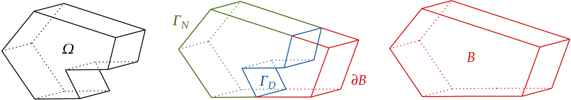
Figure 5.1: Extension of $\Omega$ (left) to a convex domain $B$ (right), with mixed boundary conditions on $\Gamma_{N}$ and $\Gamma_{D}$ (centre).

Lemma 5.4.

Assume that $\Omega\subset\mathbb{R}^{3}$ is a connected domain and that $\Gamma_{N}$ is contained in the boundary of a convex part of $\Omega$, that is, there exists a convex domain $B$ such that $\overline{\Omega}\subseteq B$ and $\Gamma_{N}\subseteq\partial B$ (see Figure 5.1). Then, for each $\boldsymbol{\xi}\in\mathbf{H}_{N}(\mathop{\mathrm{div}}\nolimits,\Omega)$, there exist $\boldsymbol{z}\in\mathbf{H}^{1}(\Omega)$ and $\boldsymbol{\chi}\in\mathbf{H}^{1}_{N}(\Omega)$ such that

$$\boldsymbol{\xi}=\boldsymbol{z}+\mathop{\mathbf{curl}}\nolimits\boldsymbol{\chi}\text{ in }\Omega\text{ and }\lVert\boldsymbol{z}\rVert_{1,\Omega}+\lVert\boldsymbol{\chi}\rVert_{1,\Omega}\lesssim\lVert\boldsymbol{\xi}\rVert_{\mathop{\mathrm{div}}\nolimits,\Omega}.$$

Next, we introduce the vector space $\mathbf{V}_{3}:=\mathbf{H}(\mathop{\mathrm{div}}\nolimits,\Omega)\cap\mathbf{H}(\mathop{\mathbf{curl}}\nolimits,\Omega)$ with corresponding local virtual space

$$\mathbf{V}_{3}^{h,k_{2}+1}(P):=\{\boldsymbol{\chi}\in\mathbf{V}_{3}(P): \,\boldsymbol{\chi}_{t}|_{\partial P}\in\mathcal{B}_{3}^{h,k_{2}+1}(\partial P),\,\mathop{\mathrm{div}}\nolimits\boldsymbol{\chi}\in\mathcal{P}_{k_{2}}(P),\mathop{\mathbf{curl}}\nolimits(\mathop{\mathbf{curl}}\nolimits\boldsymbol{\chi})\in\boldsymbol{\mathcal{R}}_{k_{2}-1}(P)\},$$

with $\mathcal{B}_{3}^{h,k_{2}}(\partial P):=\{\boldsymbol{\chi}\in(\mathcal{B}_{3})_{t}:\boldsymbol{\chi}_{f}\in\mathbf{V}_{2}^{h,k_{2}}(f),\,\forall f\in\partial P\}$. Here, $(\mathcal{B}_{3})_{t}$ is defined as the tangential component of the elements in $\mathcal{B}_{3}(\partial P)$ given for $f\in\partial P$ by

$$\mathcal{B}_{3}(\partial P):=\{\boldsymbol{\chi}\in\mathbf{L}^{2}(\partial P):\boldsymbol{\chi}|_{f}\in\mathbf{H}(\mathop{\mathrm{div}}\nolimits,f)\cap\mathbf{H}(\mathop{\mathrm{rot}}\nolimits,f),\,\forall f\in\mathcal{F}^{h},\,\boldsymbol{\chi}_{f_{1}}\cdot\boldsymbol{t}_{e}=\boldsymbol{\chi}_{f_{2}}\cdot\boldsymbol{t}_{e},\,\forall f_{1},f_{2}\in\mathcal{F}^{h}_{e},\,e\subset\partial f\}.$$

The VE space $\mathbf{V}_{2}^{h,k_{2}}(f)$ refers to the 2D edge space (see [5, Section 4]) which is a rotation by $\pi/2$ of the standard VE space for mixed problems given in Section 3. Finally, the global space $\mathbf{V}_{3}^{h,k_{2}+1}$ is given as follows

$$\mathbf{V}_{3}^{h,k_{2}+1}:=\{\boldsymbol{\chi}_{h}\in\mathbf{V}_{3}:\boldsymbol{\chi}_{h}|_{P}\in\mathbf{V}^{h,k_{2}+1}_{3}(P),\,\forall P\in\mathcal{T}^{h}\}.$$

For further details about DoFs and unisolvence we refer to [5, Section 6]. A key relation between $\mathbf{V}_{2}^{h,k_{2}}$ and $\mathbf{V}_{3}^{h,k_{2}+1}$ needed for the Helmholtz decomposition is given next and we refer to [5, Theorem 8.2] for a proof.

Lemma 5.5.

For $k_{2}\geq 1$ and $\boldsymbol{\chi}_{h}\in\mathbf{V}_{3}^{h,k_{2}+1}$, we have that $\mathop{\mathbf{curl}}\nolimits\boldsymbol{\chi}_{h}\in\mathbf{V}_{2}^{h,k_{2}}$.

Following the approach outlined in Section 4, we introduce a novel quasi-interpolation operator for the 3D VE edge space, specifically applied to $\mathbf{H}^{1}(\Omega)$ functions (see further details in Supplementary Material C).

Lemma 5.6.

Let $\boldsymbol{\chi}\in\mathbf{H}^{s_{1}+1}(\Omega)$, and $0\leq s_{2}\leq k_{2}$. Under the mesh assumptions, there exists $\mathbf{I}_{3}^{Q,k_{2}+1}\boldsymbol{\chi}\in\mathbf{V}_{3}^{h,k_{2}+1}$ such that

$$\lVert\boldsymbol{\chi}-\mathbf{I}_{3}^{Q,k_{2}+1}\boldsymbol{\chi}\rVert_{0,P}+h_{P}|\boldsymbol{\chi}-\mathbf{I}_{3}^{Q,k_{2}+1}\boldsymbol{\chi}|_{1,P}\lesssim h_{P}^{s_{2}+1}|\boldsymbol{v}|_{s_{2}+1,D(P)}.$$

Finally, we focus on the extension of the reliability and efficiency of the estimators for the 3D case. Notice that the presence of the $\mathop{\mathbf{curl}}\nolimits$ operator motivates the redefinition of the reaction-diffusion estimator as follows

$$\Xi_{2,P}^{2}:=\sum_{f\in\mathcal{F}^{h}_{\mathrm{D}}(P)}h_{f}\lVert\varphi_{\mathrm{D}}-\varphi_{h}\rVert_{0,f}^{2}+\sum_{f\in\mathcal{F}^{h}_{\mathrm{D}}(P)}h_{f}\lVert(\nabla\varphi_{\mathrm{D}}-\boldsymbol{\Pi}_{2}^{0,k_{2}}(\mathbb{M}^{-1}(\boldsymbol{\varepsilon}(\overline{\boldsymbol{u}}_{h}),{p}_{h})\boldsymbol{\Pi}_{2}^{0,k_{2}}\boldsymbol{\zeta}_{h}))\times\boldsymbol{n}\rVert_{0,f}^{2}$$

$$\quad+\sum_{f\in\mathcal{F}^{h}_{\Omega}(P)}h_{f}\lVert[\![\boldsymbol{\Pi}_{2}^{0,k_{2}}(\mathbb{M}^{-1}(\boldsymbol{\varepsilon}(\overline{\boldsymbol{u}}_{h}),{p}_{h})\boldsymbol{\Pi}_{2}^{0,k_{2}}\boldsymbol{\zeta}_{h})\times\boldsymbol{n}_{f}]\!]\rVert_{0,f}^{2}$$

$$\quad+h_{P}^{2}\lVert\boldsymbol{\Pi}_{2}^{0,k_{2}}(\mathbb{M}^{-1}(\boldsymbol{\varepsilon}(\overline{\boldsymbol{u}}_{h}),{p}_{h})\boldsymbol{\Pi}_{2}^{0,k_{2}}\boldsymbol{\zeta}_{h})-\nabla\varphi_{h}\rVert_{0,P}^{2}+h_{P}^{2}\lVert\mathop{\mathbf{curl}}\nolimits(\boldsymbol{\Pi}_{2}^{0,k_{2}}(\mathbb{M}^{-1}(\boldsymbol{\varepsilon}(\overline{\boldsymbol{u}}_{h}),{p}_{h})\boldsymbol{\Pi}_{2}^{0,k_{2}}\boldsymbol{\zeta}_{h}))\rVert_{0,P}^{2}.$$

On the other hand, $\Theta_{1,P}$ and the remaining terms of $\Theta_{2,P}$ are defined analogously to (4.1) replacing edges $e$ and polygons $E$ with faces $f$ and polyhedrons $P$, respectively. Following the techniques from Section 4 and the the quasi-interpolator $\mathbf{I}_{1}^{Q,k_{1}}$ from Lemma 5.1, implies Lemma 4.16. In turn, Lemma 4.22 is a consequence of bubble functions in polyhedra and faces (see [15, Lemmas 8,9]). Next, we recall integration by parts formulae involving $\mathop{\mathbf{curl}}\nolimits(\boldsymbol{\chi}-\boldsymbol{\chi}_{h})$, with $\boldsymbol{\chi}\in\mathbf{H}^{1}_{N}(\Omega)$ and $\boldsymbol{\chi}_{h}:=\mathbf{I}_{3}^{Q,k_{2}+1}(\boldsymbol{\chi})\in\mathbf{V}_{3}^{h,k_{2}+1}$ [30, Equation 2.17, Theorem 2.11]:

(5.1) $$\sum_{f\in\mathcal{F}^{h}_{D}}\langle\mathop{\mathbf{curl}}\nolimits(\boldsymbol{\chi}-\boldsymbol{\chi}_{h}),\varphi_{\mathrm{D}}\rangle_{f} =-\sum_{f\in\mathcal{F}^{h}_{D}}\langle\boldsymbol{\chi}-\boldsymbol{\chi}_{h},\nabla\varphi_{\mathrm{D}}\times\boldsymbol{n}_{f}\rangle_{f},$$

$$\int_{P}\boldsymbol{\Pi}_{2}^{0,k_{2}}(\mathbb{M}^{-1}(\boldsymbol{\varepsilon}(\overline{\boldsymbol{u}}_{h}),{p}_{h})\boldsymbol{\Pi}_{2}^{0,k_{2}}\boldsymbol{\zeta}_{h})\cdot\mathop{\mathbf{curl}}\nolimits(\boldsymbol{\chi}-\boldsymbol{\chi}_{h}) =\sum_{f\in\mathcal{F}^{h}(P)}\langle\boldsymbol{\chi}-\boldsymbol{\chi}_{h},\boldsymbol{\Pi}_{2}^{0,k_{2}}(\mathbb{M}^{-1}(\boldsymbol{\varepsilon}(\overline{\boldsymbol{u}}_{h}),{p}_{h})\boldsymbol{\Pi}_{2}^{0,k_{2}}\boldsymbol{\zeta}_{h})\times\boldsymbol{n}_{f}\rangle_{f}$$

$$\,+\int_{P}\mathop{\mathbf{curl}}\nolimits\left(\boldsymbol{\Pi}_{2}^{0,k_{2}}(\mathbb{M}^{-1}(\boldsymbol{\varepsilon}(\overline{\boldsymbol{u}}_{h}),{p}_{h})\boldsymbol{\Pi}_{2}^{0,k_{2}}\boldsymbol{\zeta}_{h})\right)\cdot(\boldsymbol{\chi}-\boldsymbol{\chi}_{h}).$$

From here, Lemma 4.19 follows from Lemma 5.4, and Lemma 5.6. Finally, since $\mathop{\mathbf{curl}}\nolimits(\nabla\varphi)=\boldsymbol{0}$, Lemma 4.24 can be extended again using bubble functions techniques and the integration by parts presented in (5.1). Therefore, Theorem 4.21 and Theorem 4.26 hold also in the 3D case.

6 Numerical tests

In this section, we present numerical results illustrating the properties of the robust estimator from Section 4 and show the optimal behaviour of the associated adaptive algorithm under different polygonal convex meshes and polynomial orders. We also use L-shaped and Australia-shaped domains to illustrate the capability of capturing singularities in non-convex domains. Finally, we show some 3D tests.

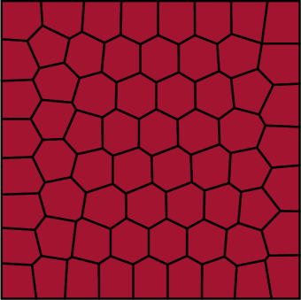
(a) Voronoi.

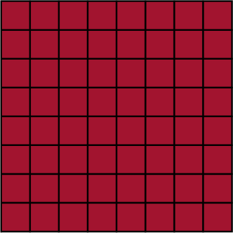
(b) Square.

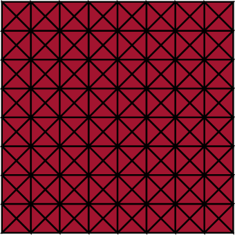
(c) Crossed.

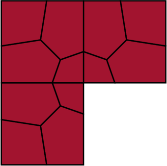
(d) L.

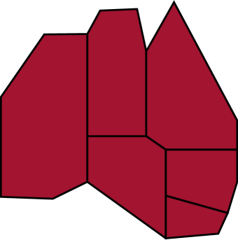
(e) Australia.

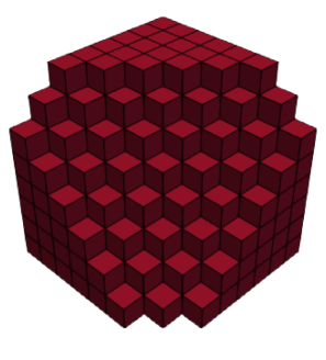
(f) Cube.

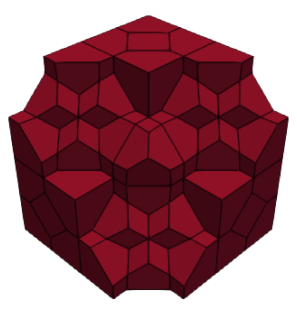
(g) Nove.

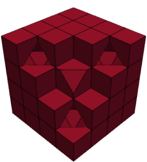
(h) Octa.

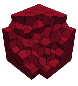
(i) Voro.

Figure 6.1: An illustration of the distinct meshes used in the examples.

The error will be computed as usual in the VEM framework using the local polynomial approximation of the solution as follows $\overline{\textnormal{e}}_{*}^{2}=\lVert(\boldsymbol{u}-\boldsymbol{\Pi}_{1}^{\boldsymbol{\varepsilon},k_{1}}\boldsymbol{u}_{h},{p}-{p}_{h})\rVert_{\mathbf{V}_{1}^{h,k_{1}}\times\mathrm{Q}_{1}^{h,k_{1}}}^{2}+\lVert(\boldsymbol{\zeta}-\boldsymbol{\Pi}_{2}^{0,k_{2}}\boldsymbol{\zeta}_{h},\varphi-\varphi_{h})\rVert_{\mathbf{V}_{2}^{h,k_{2}}\times\mathrm{Q}_{2}^{h,k_{2}}}^{2}.$ The numerical implementation has been done with the library VEM++ [18]. We separately implemented the elasticity and reaction-diffusion equations for arbitrary orders $k_{1}$ and $k_{2}$, respectively. Then, the nonlinear coupled problem (3.2) is solved with an optimised Picard iteration, following the same structure as in the fixed-point analysis from [31], with a tolerance of $10^{-6}$. In this optimised version, the blocks corresponding to the coupling terms ($G_{1}^{\varphi_{h}}(\cdot)$ and $a_{2}^{\overline{\boldsymbol{u}}_{h},{p},h}(\cdot,\cdot)$) are the only ones that are reconstructed on each fixed point iteration. We recall that the elasticity and reaction-diffusion equations have sufficiently smooth forcing and source terms that will be manufactured according to the given exact solutions. The non-homogeneous boundary conditions require a slight modification of the right-hand side functionals as well as the estimator boundary term $\Xi_{1,E}$ regarding $\Gamma_{\mathrm{N}}$. The experimental order of convergence $r(\cdot)$ applied to either error $\overline{\textnormal{e}}_{*}$ or estimator $\Theta$ and the effectivity index (following Theorem 4.21) of the refinement $1\leq j$ are computed from the formulae $r(\cdot)^{j+1}=-d\log\left((\cdot)^{j+1}/(\cdot)^{j}\right)/\log\left(\textnormal{DOF}_{*}^{j+1}/\textnormal{DOF}_{*}^{j}\right)$ and $\textnormal{eff}^{j}=\Theta^{j}/\overline{\textnormal{e}}_{*}^{j}$, with $\textnormal{DOF}_{*}$ indicating the total number of DoFs. In turn, the stabilisation term $S_{1}^{E}(\boldsymbol{u}_{h},\boldsymbol{v}_{h})$ follows the “diagonal recipe” introduced in [7] (weighted by $2\mu$) and $S_{2}^{\overline{\boldsymbol{u}}_{h},{p}_{h},E}(\boldsymbol{\zeta}_{h},\boldsymbol{\xi}_{h})$ have into account the nonlinearity $\mathbb{M}^{-1}(\overline{\boldsymbol{u}}_{h},{p}_{h})$ as in [31].

The adaptive algorithm follows the usual strategy: $\textnormal{SOLVE}\rightarrow\textnormal{ESTIMATE}\rightarrow\textnormal{MARK}\rightarrow\textnormal{REFINE}$. The first three steps are performed inside VEM++, exploiting the efficiency capabilities of C++. For the REFINE step, we use the Matlab-based method from [49], which connects edge midpoints to the polygon barycentre (in 2D). In turn, the adaptive refinement used in this paper relies on the library p4est [14] executed through the module GridapP4est of the Julia package Gridap [3]. The VEM++ code is executed through Matlab/Julia (2D/3D, respectively), generating a list of elements to refine, which is then processed by the refinement routine. These refinement routines restrict the mesh elements to convex polygons in 2D and cubes (with hanging nodes/faces) in 3D. However, we recall that this procedure is independent of the SOLVE, ESTIMATE, and MARK stages. Therefore, the implementation can be extended to general star-shaped polygons with more general refinement routines. For the MARK procedure we follow a Dörfler/Bulk strategy, marking the subset of mesh elements $\mathcal{K}\subseteq\mathcal{T}^{h}$ with the largest estimated errors such that for $\delta=\frac{1}{2}\in[0,1]$, we have $\delta\sum_{E\in\mathcal{T}^{h}}\Theta_{E}^{2}\leq\sum_{E\in\mathcal{K}}\Theta_{E}^{2}.$

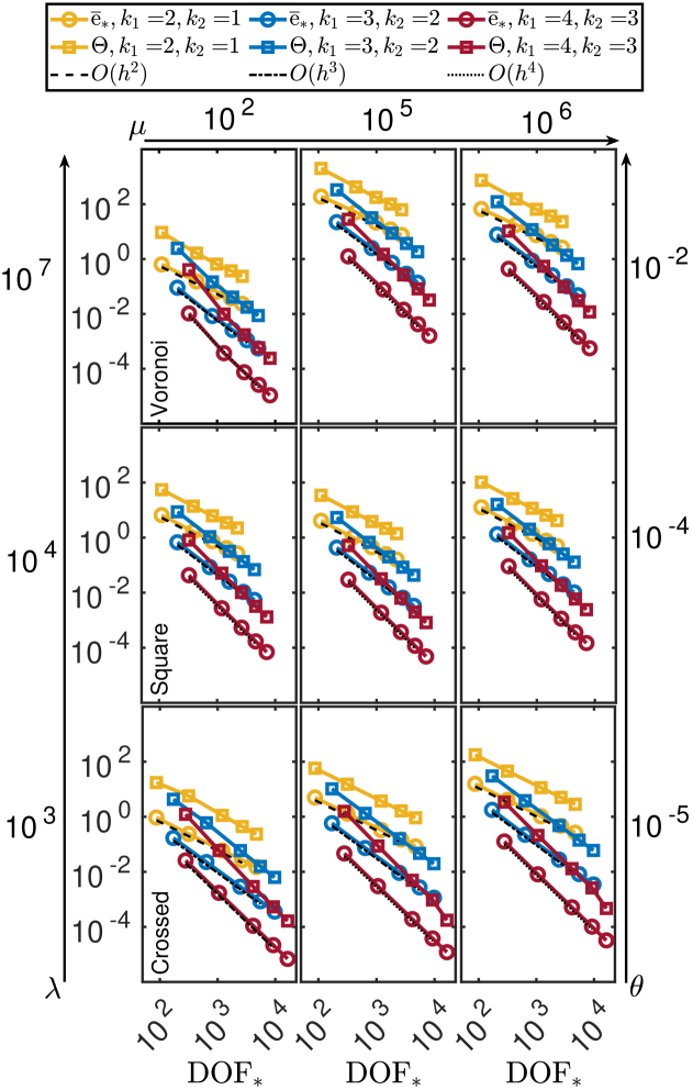
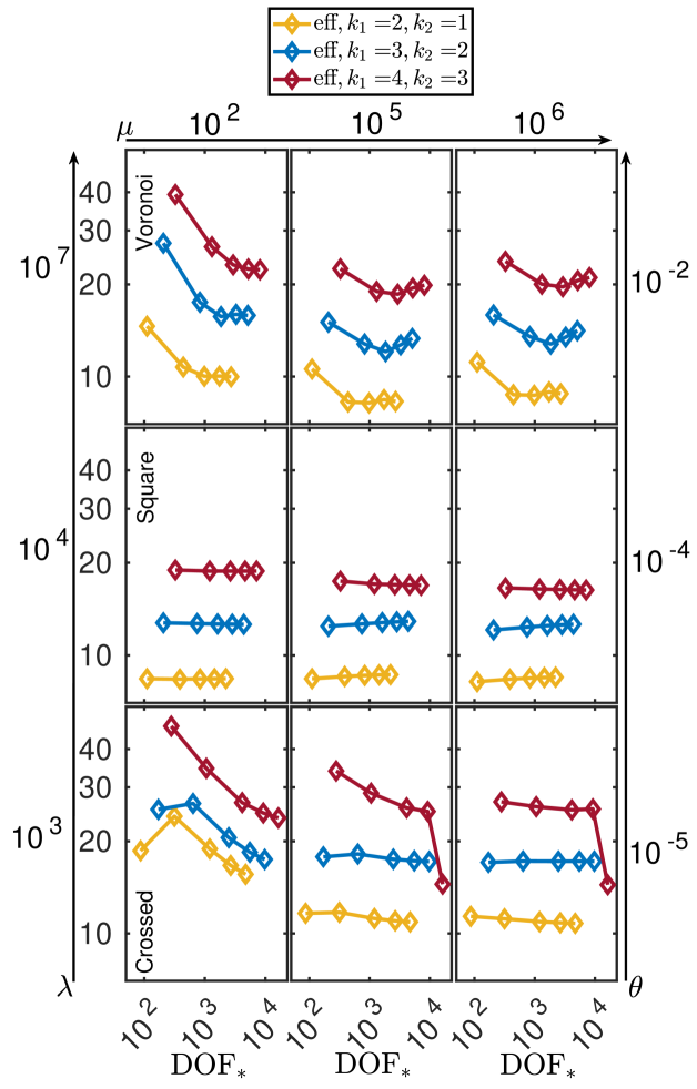
Figure 6.2: Example 1. Behaviour of the error $\overline{\textnormal{e}}_{*}$, estimator $\Theta$ (left), and effectivity index eff (right) under uniform refinement across various meshes, polynomial orders, and parameter selections.

6.1 Example 1: Robust behaviour of the estimator under uniform refinement

We consider the meshes in Fig 6.1 for the unit square domain $\Omega=(0,1)^{2}$ with Dirichlet part $\Gamma_{\mathrm{D}}=\{(x,y)\in\partial\Omega\colon x=0\;\text{or}\;y=0\}$, and Neumann part $\Gamma_{\mathrm{N}}=\partial\Omega\setminus\Gamma_{\mathrm{D}}$. We explore different polynomial degrees for the elasticity and reaction-diffusion equations given by $k_{1}=2,3,4$ and $k_{2}=1,2,3$. Smooth manufactured solutions and nonlinearities are set as

$$\boldsymbol{u}(x,y)=5^{-1}\left(x^{2}+x\cos(x)\sin(y),y^{2}+x\cos(y)\sin(x)\right)^{\tt t},\quad\varphi(x,y)=\cos(\pi y)+\sin(\pi x)+x^{2}+y^{2},$$

$$\ell(\varphi)=\varphi,\quad\mathbb{M}(\boldsymbol{\varepsilon}(\boldsymbol{u}),p)=10^{-1}\exp{\left[-10^{-8}\mathop{\mathrm{tr}}\nolimits(2\mu\boldsymbol{\varepsilon}(\boldsymbol{u})-p\mathbb{I})\right]}\mathbb{I}.$$

As usual, the exact displacement $\boldsymbol{u}$ and concentration $\varphi$ are used to compute exact Herrmann pressure ${p}$ and total flux $\boldsymbol{\zeta}$, as well as appropriate forcing term, source, and non-homogeneous traction, displacement, and flux boundary data. Finally, we use the parameter value $M=12$.

The results in Figure 6.2 demonstrate robust optimal convergence rates predicted by Theorem 3.4 for $\overline{\textnormal{e}}_{*}$ and $\Theta$ under uniform refinement for a variation in the involved parameters $\mu,\lambda,\theta$. In addition, Figure 6.2 shows the effectivity index for the different experiments, here we can observe that it oscillates around a fixed number for each case, confirming the reliability of the estimator given by Theorem 4.21.

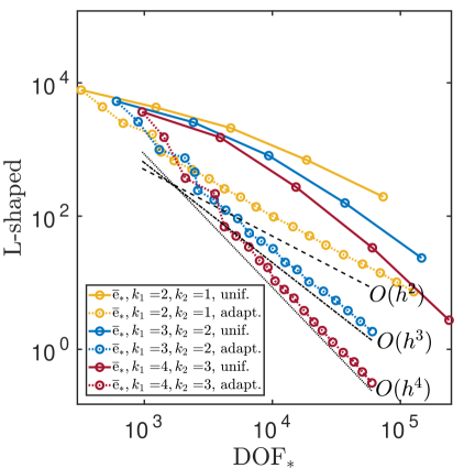
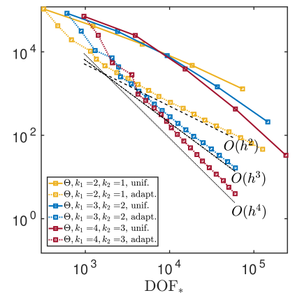
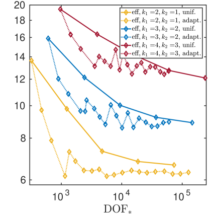
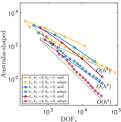
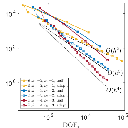
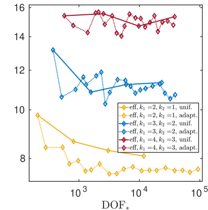
Figure 6.3: Example 2. Behaviour of $\overline{\textnormal{e}}_{*}$ (left column), $\Theta$ (middle column), and eff (right column) under uniform and adaptive refinement on L-shape (top row) and Australia-shape (bottom row) domains for a variety polynomial orders.

6.2 Example 2: Non-smooth solution on non-convex domains

In this case, we set an initial polygonal discretisation for the L-shaped domain $\Omega=(-1,1)^{2}\setminus[0,1)\times[0,-1)$ with boundary conditions defined on $\Gamma_{\mathrm{N}}=\{(x,y)\in\partial\Omega:x=-1,\,y=1\}$ and $\Gamma_{\mathrm{D}}=\partial\Omega\setminus\Gamma_{N}$ (see Figure 1(d)). In contrast, the Australia-shaped domain is set to fit inside the unit square where each element in the initial discretisation represents the in-land states (See Figure 1(e)), the further east edge coincides with $x=0$ where $\Gamma_{\mathrm{N}}$ is defined, whereas $\Gamma_{\mathrm{D}}=\partial\Omega\setminus\Gamma_{N}$.

The non-smooth manufactured solutions and the non-linear terms are set as follows

$$\boldsymbol{u}(x,y)=\left(\frac{(x-1.0)(y-1.0)}{\left(x-x_{*}\right)^{2}+\left(y-y_{*}\right)^{2}},\frac{(x+1.0)(y+1.0)}{\left(x-x_{*}\right)^{2}+\left(y-y_{*}\right)^{2}}\right)^{\tt t},\quad\ell(\varphi)=2+\frac{\varphi^{2}}{1+\varphi^{2}},$$

$$\varphi(x,y)=\frac{(x-1.0)(x+1.0)(y-1.0)(y+1.0)}{\left(x-x_{*}\right)^{2}+\left(y-y_{*}\right)^{2}},\quad\mathbb{M}(\boldsymbol{\varepsilon}(\boldsymbol{u}),p)=\left(1+\frac{10^{-5}}{\mathop{\mathrm{tr}}\nolimits(2\mu\boldsymbol{\varepsilon}(\boldsymbol{u})-p\mathbb{I})}\right)\mathbb{I},$$

with parameter values $\mu=1.4286\times 10^{3}$, $\lambda=357.1429$, $\theta=10^{-3}$, and $M=2$. Displacement and concentration admit a singularity depending on the selection of the point $(x_{*},y_{*})^{\tt t}$. For the L-shaped domain we set $(x_{*},y_{*})^{\tt t}=(10^{-1},-10^{-1})^{\tt t}$, expecting high gradients close to the reentrant corner. In contrast, the Australian-shape domain expects high gradients near the location of Melbourne, i.e., $(x_{*},y_{*})^{\tt t}=(8.5\times 10^{-1},-10^{-1})^{\tt t}$.

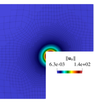
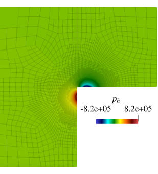
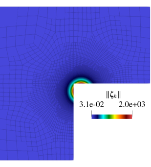
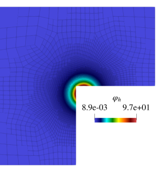
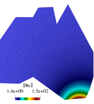
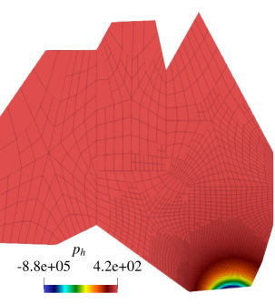
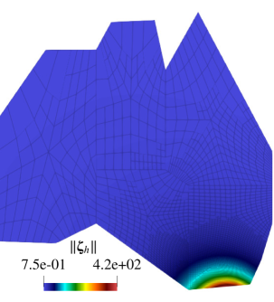
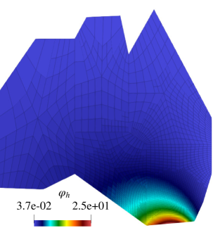
Figure 6.4: Example 2. Snapshots of the interest variables on the L-shape (top) and Australia-shape (bottom) meshes are shown for polynomial degrees $k_{1}=2$ and $k_{2}=1$ after 19 refinement steps.

Figure 6.3 shows the behaviour of $\overline{\textnormal{e}}_{h}$, $\Theta$, and eff under uniform and adaptive refinement for different polynomial degrees. As expected, the error decreases faster (optimally) under the adaptive procedure, and the effectivity index remains bounded, confirming the robustness of the estimator. Figure 6.4 displays approximate solutions after 19 adaptive mesh refinement steps according to $\Theta$. Most of the refinement occurs around the singularities, demonstrating how the method identifies regions where accuracy deteriorates.

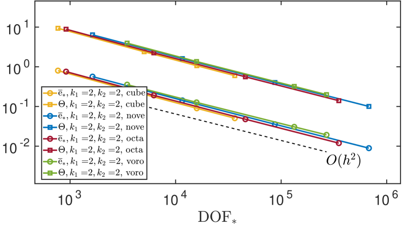
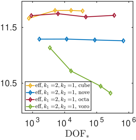
Figure 6.5: Example 3. Behaviour of the error $\overline{\textnormal{e}}_{*}$, estimator $\Theta$ (left), and effectivity index eff (right) under uniform refinement across various meshes with $k_{1}=2$ and $k_{2}=2$.

6.3 Example 3: Behaviour of estimator under uniform refinement in 3D

We consider the meshes in Figure 6.1 for the unit cube domain $\Omega=(0,1)^{3}$ with Dirichlet part $\Gamma_{\mathrm{D}}=\{(x,y,z)\in\partial\Omega\colon x=0\;\text{or}\;y=0\;\text{or}\;z=0\}$, and Neumann part $\Gamma_{\mathrm{N}}=\partial\Omega\setminus\Gamma_{\mathrm{D}}$. We set the polynomial degrees to $k_{1}=2$ and $k_{2}=2$ for the discrete spaces defined in Section 5.2, noting that the implementation presented in this paper supports arbitrary polynomial degrees. For this example, we fix the adimensional parameters as $\mu=10^{2}$, $\lambda=10^{3}$, $\theta=10^{-3}$, and $M=20$. On the other hand, the manufactured solutions and non-linear terms are given as follows

$$\boldsymbol{u}(x,y,z)=5^{-1}\left(x^{2}+x\cos(x)\sin(y),y^{2}+x\cos(y)\sin(x),z^{2}+x\cos(x)\cos(y)\right)^{\tt t},$$

$$\varphi(x,y,z)=\cos(\pi y)+\sin(\pi x)+x^{2}+y^{2}+z^{2},\;\ell(\varphi)=\varphi+\varphi^{2},\;\mathbb{M}(\boldsymbol{\varepsilon}(\boldsymbol{u}),p)=10^{-1}\exp{\left[-10^{-4}\mathop{\mathrm{tr}}\nolimits(2\mu\boldsymbol{\varepsilon}(\boldsymbol{u})-p\mathbb{I})\right]}\mathbb{I}.$$

We recall that the right-hand sides and non-homogeneous boundary conditions are introduced in the computations according to these terms. The results reported in Figure 6.5 indicate optimal convergence rates for $k_{1}=2$ and $k_{2}=2$, as in [42]. In addition, the effectivity index remains bounded, which confirms the reliability and efficiency of the estimator (see Theorem 4.21 and Theorem 4.26).

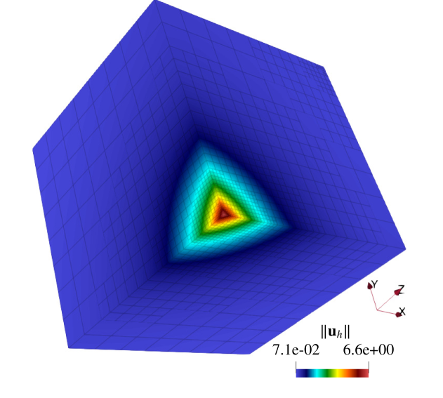
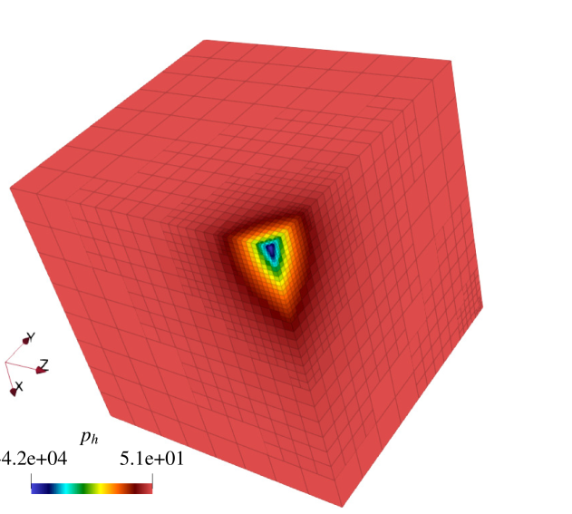
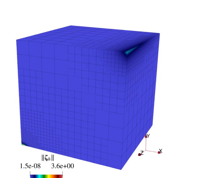
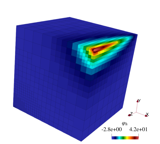
Figure 6.6: Example 4. Approximate solutions obtained with polynomial degrees $k_{1}=2$ and $k_{2}=2$ after 14 adaptive refinements.

6.4 Example 4: Adaptivity in 3D

For this example, we consider the unit cube domain $\Omega=(0,1)^{3}$ with Dirichlet part $\Gamma_{\mathrm{D}}=\{(x,y,z)\in\partial\Omega\colon x=0\;\text{or}\;y=0\;\text{or}\;z=0\}$, and Neumann part $\Gamma_{\mathrm{N}}=\partial\Omega\setminus\Gamma_{\mathrm{D}}$. The starting mesh is defined by $4^{3}$ cubes. Here we fix the adimensional parameters as $\mu=10^{2}$, $\lambda=10^{3}$, $\theta=10^{-3}$, and $M=100$. The non-smooth manufactured solutions and non-linear terms are given as follows

$$\boldsymbol{u}(x,y,z)=5^{-1}\left(\left((x+0.1)^{2}+(y+0.1)^{2}+(z-1.1)^{2}\right)^{-1},z\cos(x)\sin(y),x\cos(z)\sin(y)\right)^{\tt t},$$

$$\varphi(x,y,z)=xyz\left((x-1.1)^{2}+(y-1.1)^{2}\right)^{-1},\quad\ell(\varphi)=10^{-2}\varphi,\quad\mathbb{M}(\boldsymbol{\varepsilon}(\boldsymbol{u}),p)=10^{-3}\exp{\left[-10^{-4}\mathop{\mathrm{tr}}\nolimits(2\mu\boldsymbol{\varepsilon}(\boldsymbol{u})-p\mathbb{I})\right]}\mathbb{I}.$$

The first displacement component has a singularity close to the point $(x,y,z)^{\tt t}=(0,0,1)^{\tt t}$. In addition, the concentration $\varphi$ has a high gradient close to the line $(x,y,z)^{\tt t}=(1,1,1-t)^{\tt t}$ for $t\in\mathbb{R}$. The results reported in Figure 6.7 show optimal convergence s as predicted in [42]. Moreover, we observe that the adaptive refinement outperforms the uniform refinement. In addition, the effectivity index remains bounded, confirming the robustness of the estimator proved in Theorems 4.21 and 4.26. Finally, Figure 6.6 shows snapshots of the approximate solutions on a mesh after 15 refinement steps. The method is able to capture the expected solution singularities.

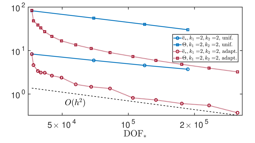
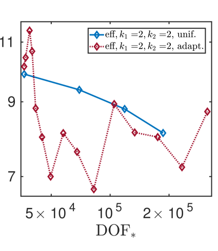
Figure 6.7: Example 4. Behaviour of the error $\overline{\textnormal{e}}_{*}$, estimator $\Theta$ (left), and effectivity index eff (right) under adaptive and uniform refinement for the lowest-order case.

Supplementary Material

This document presents auxiliary results to accompany the manuscript “A posteriori error analysis of robust a virtual element method for stress-assisted diffusion problems” by F. Dassi, R. Khot, A.E. Rubiano, and R. Ruiz-Baier.

Appendix A Proof of Theorem 2.2

Proof A.1.

The triangle inequality and the second Brezzi condition (2.3b) lead to

$$\lVert(u,p)\rVert_{V\times Q}\leq\lVert u\rVert_{V}+\frac{1}{\beta}\sup_{v\in V}\frac{\mathcal{A}(u,p;v,0)-a(u,v)}{{\lVert v\rVert}_{V}}+t|p|_{c}.$$

Note that $t|p|_{c}\leq\left(a(u,u)+t^{2}c(p,p)\right)^{\frac{1}{2}}=\left(\mathcal{A}(u,p;u,-p)\right)^{\frac{1}{2}}$, which together with the continuity of $a(\cdot,\cdot)$ yields

$$\lVert(u,p)\rVert_{V\times Q}\leq\left(1+\lVert a\rVert\right)\lVert u\rVert_{V}+\frac{1}{\beta}\sup_{(v,q)\in V\times Q}\frac{\mathcal{A}(u,p;v,q)}{{\lVert(v,q)\rVert_{V\times Q}}}+\left(A(u,p;u,-p)\right)^{\frac{1}{2}}.$$

The Braess condition (2.3c) implies that

$$\lVert(u,p)\rVert_{V\times Q} \leq\left(\frac{1+\lVert a\rVert}{\gamma}\right)\sup_{(v,q)\in V\times Q}\frac{a(u,v)+b(u,q)}{\lVert(v,q)\rVert_{V\times Q}}+\frac{1}{\beta}\sup_{(v,q)\in V\times Q}\frac{\mathcal{A}(u,p;v,q)}{{\lVert(v,q)\rVert_{V\times Q}}}+\left(\mathcal{A}(u,p;u,-p)\right)^{\frac{1}{2}}.$$

Since $a(u,v)+b(u,q)=\mathcal{A}(u,p;v,q)-b(v,p)+t^{2}c(p,q)$, we readily see that

$$\lVert(u,p)\rVert_{V\times Q} \leq\left(\frac{1+\lVert a\rVert}{\gamma}+\frac{1}{\beta}\right)\sup_{(v,q)\in V\times Q}\frac{A(u,p;v,q)}{\lVert(v,q)\rVert_{V\times Q}}+\left(1+\frac{1+\lVert a\rVert}{\gamma}\right)\left(\mathcal{A}(u,p;u,-p)\right)^{\frac{1}{2}}.$$

Given that for all $0<x,y,z$ the inequality $x\leq y+z$ implies that $x\leq 2y+\frac{z^{2}}{x}$, we have

$$\lVert(u,p)\rVert_{V\times Q} \leq 2\left(\frac{1+\lVert a\rVert}{\gamma}+\frac{1}{\beta}\right)\sup_{(v,q)\in V\times Q}\frac{\mathcal{A}(u,p;v,q)}{\lVert(v,q)\rVert_{V\times Q}}+\left(1+\frac{1+\lVert a\rVert}{\gamma}\right)^{2}\frac{\mathcal{A}(u,p;u,-p)}{\lVert(u,p)\rVert_{V\times Q}}.$$

The proof concludes by taking the supremum for all $(v,q)\in V\times Q$.

Appendix B Proof of Proposition 5.1

Proof B.1.

Step 1 (Existence of interpolation in the space $\widetilde{\mathbf{V}}_{1}^{h,k_{1}}$). Let $P\in\mathcal{T}^{h}$, we start considering the super-enhanced version of the enhanced VE space $\widetilde{\boldsymbol{\mathcal{B}}}^{h,k_{1}}_{1}(f)$ from [15] which locally solves a Poisson problem with Dirichlet boundary conditions. Let $\mathbf{I}_{1}^{C,k_{1}}\boldsymbol{v}\in\mathbf{H}^{1}_{D}(\Omega)$ be the Clément-type VE interpolation in $\widetilde{\boldsymbol{\mathcal{B}}}^{h,k_{1}}_{1}(f)$ satisfying the following estimate for all $P\in\mathcal{T}^{h}$ (see [15, Theorem 11])

(B.1) $$\lVert\boldsymbol{v}-\mathbf{I}_{1}^{C,k_{1}}\boldsymbol{v}\rVert_{0,P}+h_{P}\lVert\boldsymbol{\varepsilon}(\boldsymbol{v}-\mathbf{I}_{1}^{C,k_{1}}\boldsymbol{v})\rVert_{0,P}\lesssim h_{P}^{s_{1}+1}|\boldsymbol{v}|_{s_{1}+1,D(P)}.$$

Let $\boldsymbol{v}_{\pi}=\boldsymbol{\Pi}_{1}^{\boldsymbol{\varepsilon},k_{1}}\boldsymbol{v}$ be the polynomial approximation of $\boldsymbol{v}$. The decomposition $\boldsymbol{\mathcal{P}}_{k_{1}-2}(P)=\boldsymbol{\mathcal{G}}_{k_{1}-2}(P)\oplus\boldsymbol{\mathcal{G}}_{k_{1}-2}^{\oplus}(P)$ guarantees the existence of $p_{\pi}\in\mathcal{P}_{k_{1}-1}(P)$ and $\boldsymbol{g}_{\pi}^{\oplus}\in\boldsymbol{\mathcal{G}}_{k_{1}-2}^{\oplus}(P)$ such that

(B.2) $$-2\mu\mathop{\mathbf{div}}\nolimits\boldsymbol{\varepsilon}(\boldsymbol{v}_{\pi})=\nabla p_{\pi}+\boldsymbol{g}_{\pi}^{\oplus}.$$

For $q_{k_{1}-1}|_{P}=\Pi_{1}^{0,k_{1}-1}(\mathop{\mathrm{div}}\nolimits\mathbf{I}_{1}^{C,k_{1}}\boldsymbol{v})$, we introduce the following Stokes problem for all $P\in\mathcal{T}^{h}$ as

(B.3) $$\begin{cases}-2\mu\mathop{\mathbf{div}}\nolimits(\boldsymbol{\varepsilon}(\widetilde{\boldsymbol{v}}_{I}))-\nabla s=\boldsymbol{g}_{\pi}^{\oplus}&\quad\text{in}\;P,\\ \mathop{\mathrm{div}}\nolimits\widetilde{\boldsymbol{v}}_{I}=q_{k_{1}-1}&\quad\text{in}\;P,\\ \widetilde{\boldsymbol{v}}_{I}=\mathbf{I}_{1}^{C,k_{1}}\boldsymbol{v}&\quad\text{on}\;\partial P.\end{cases}$$

Observe that $\widetilde{\boldsymbol{v}}_{I}\in\widetilde{\mathbf{V}}_{1}^{h,k_{1}}(P)$ from the definition of $\widetilde{\mathbf{V}}_{1}^{h,k_{1}}(P)$. This and $\widetilde{\boldsymbol{v}}_{I}=\mathbf{I}_{1}^{C,k_{1}}\boldsymbol{v}\in\mathbf{V}_{1}$ on each boundary of $P$ imply that $\widetilde{\boldsymbol{v}}_{I}\in\widetilde{\mathbf{V}}_{1}^{h,k_{1}}$.

Step 2 (Error estimate). Note that (B.2) imply that $\boldsymbol{v}_{\pi}$ solves the following local Stokes problem

(B.4) $$\begin{cases}-2\mu\mathop{\mathbf{div}}\nolimits(\boldsymbol{\varepsilon}(\boldsymbol{v}_{\pi}))-\nabla p_{\pi}=\boldsymbol{g}_{\pi}^{\oplus}&\quad\text{in}\;P,\\ \mathop{\mathrm{div}}\nolimits\boldsymbol{v}_{\pi}=\mathop{\mathrm{div}}\nolimits\boldsymbol{v}_{\pi}&\quad\text{in}\;P,\\ \boldsymbol{v}_{\pi}=\boldsymbol{v}_{\pi}&\quad\text{on}\;\partial P.\end{cases}$$

On the other hand, we define the auxiliary problem

(B.5) $$\begin{cases}-2\mu\mathop{\mathbf{div}}\nolimits(\boldsymbol{\varepsilon}(\widetilde{\boldsymbol{v}}))-\nabla\widetilde{s}=\boldsymbol{g}_{\pi}^{\oplus}&\quad\text{in}\;P,\\ \mathop{\mathrm{div}}\nolimits\widetilde{\boldsymbol{v}}=\mathop{\mathrm{div}}\nolimits\mathbf{I}_{1}^{C,k_{1}}\boldsymbol{v}&\quad\text{in}\;P,\\ \widetilde{\boldsymbol{v}}=\mathbf{I}_{1}^{C,k_{1}}\boldsymbol{v}&\quad\text{on}\;\partial P.\end{cases}$$

Then, subtracting (B.4) and (B.5) lead to

(B.6) $$\begin{cases}-2\mu\mathop{\mathbf{div}}\nolimits(\boldsymbol{\varepsilon}(\boldsymbol{v}_{\pi}-\widetilde{\boldsymbol{v}}))-\nabla(p_{\pi}-\widetilde{s})=\boldsymbol{0}&\quad\text{in}\;P,\\ \mathop{\mathrm{div}}\nolimits(\boldsymbol{v}_{\pi}-\widetilde{\boldsymbol{v}})=\mathop{\mathrm{div}}\nolimits(\boldsymbol{v}_{\pi}-\mathbf{I}_{1}^{C,k_{1}}\boldsymbol{v})&\quad\text{in}\;P,\\ \boldsymbol{v}_{\pi}-\widetilde{\boldsymbol{v}}=\boldsymbol{v}_{\pi}-\mathbf{I}_{1}^{C,k_{1}}\boldsymbol{v}&\quad\text{on}\;\partial P.\end{cases}$$

Since $\boldsymbol{z}-(\boldsymbol{v}_{\pi}-\widetilde{\boldsymbol{v}})\in\mathbf{H}^{1}_{0}(P)$ for any $\boldsymbol{z}\in\mathbf{H}^{1}(P)$ with $\mathop{\mathrm{div}}\nolimits\boldsymbol{z}=\mathop{\mathrm{div}}\nolimits(\boldsymbol{v}_{\pi}-\mathbf{I}_{1}^{C,k_{1}}\boldsymbol{v})$ in $P$ and $\boldsymbol{z}=\boldsymbol{v}_{\pi}-\mathbf{I}_{1}^{C,k_{1}}\boldsymbol{v}$ on $\partial P$, an integration by parts twice and (B.6) show

$$2\mu\int_{P}\boldsymbol{\varepsilon}(\boldsymbol{v}_{\pi}-\widetilde{\boldsymbol{v}}):\boldsymbol{\varepsilon}(\boldsymbol{z}-(\boldsymbol{v}_{\pi}-\widetilde{\boldsymbol{v}}))=\int_{P}\nabla(p_{\pi}-\widetilde{s})\cdot(\boldsymbol{z}-(\boldsymbol{v}_{\pi}-\widetilde{\boldsymbol{v}}))=-\int_{P}(p_{\pi}-\widetilde{s})\mathop{\mathrm{div}}\nolimits(\boldsymbol{z}-(\boldsymbol{v}_{\pi}-\widetilde{\boldsymbol{v}}))=0.$$

This results in $\lVert\boldsymbol{\varepsilon}(\boldsymbol{v}_{\pi}-\widetilde{\boldsymbol{v}})\rVert_{0,P}\leq\lVert\boldsymbol{\varepsilon}(\boldsymbol{z})\rVert_{0,P}$ and hence for $\boldsymbol{z}=\boldsymbol{v}_{\pi}-\mathbf{I}_{1}^{C,k_{1}}\boldsymbol{v}$ we have

(B.7) $$\lVert\boldsymbol{\varepsilon}(\boldsymbol{v}_{\pi}-\widetilde{\boldsymbol{v}})\rVert_{0,P}\leq\lVert\boldsymbol{\varepsilon}(\boldsymbol{v}_{\pi}-\mathbf{I}_{1}^{C,k_{1}}\boldsymbol{v})\rVert_{0,P}\leq\lVert\boldsymbol{\varepsilon}(\boldsymbol{v}-\boldsymbol{v}_{\pi})\rVert_{0,P}+\lVert\boldsymbol{\varepsilon}(\boldsymbol{v}-\mathbf{I}_{1}^{C,k_{1}}\boldsymbol{v})\rVert_{0,P}\lesssim h_{P}^{s_{1}}|\boldsymbol{v}|_{s_{1}+1,D(P)},$$

where the triangle inequality, $\lVert\boldsymbol{\varepsilon}(\cdot)\rVert_{0,P}\leq|\cdot|_{1,P}$, Lemma 3.1 and (B.1) were applied. Next, to estimate $\widetilde{\boldsymbol{v}}-\widetilde{\boldsymbol{v}}_{I}$ we consider the auxiliary problem arising from subtracting (B.5) and (B.3)

$$\begin{cases}-2\mu\mathop{\mathbf{div}}\nolimits(\boldsymbol{\varepsilon}(\widetilde{\boldsymbol{v}}-\widetilde{\boldsymbol{v}}_{I}))-\nabla(\widetilde{s}-s)=\boldsymbol{0}&\quad\text{in}\;P,\\ \mathop{\mathrm{div}}\nolimits(\widetilde{\boldsymbol{v}}-\widetilde{\boldsymbol{v}}_{I})=\mathop{\mathrm{div}}\nolimits(\mathbf{I}_{1}^{C,k_{1}}\boldsymbol{v})-q_{k-1}&\quad\text{in}\;P,\\ \widetilde{\boldsymbol{v}}-\widetilde{\boldsymbol{v}}_{I}=\boldsymbol{0}&\quad\text{on}\;\partial P.\end{cases}$$

Given a star-shaped polyhedral domain $P$ with respect to a ball $B$, the mesh assumptions lead to $|P||B|^{-1}\leq\rho^{-3}$ in 3D (see e.g. [19]). This and [21, Theorem 3.2] imply that there exists a universal positive constant depending only on the mesh regularity parameter $\rho$ and the dimension $d$ (but independent of $P$) such that

(B.8) $$\lVert\boldsymbol{\varepsilon}(\widetilde{\boldsymbol{v}}-\widetilde{\boldsymbol{v}}_{I})\rVert_{0,P}\leq|\widetilde{\boldsymbol{v}}-\widetilde{\boldsymbol{v}}_{I}|_{1,P}\lesssim\lVert\mathop{\mathrm{div}}\nolimits(\mathbf{I}_{1}^{C,k_{1}}\boldsymbol{v})-\Pi_{1}^{0,k_{1}-1}\mathop{\mathrm{div}}\nolimits(\mathbf{I}_{1}^{C,k_{1}}\boldsymbol{v})\rVert_{0,P}.$$

Note that the triangle inequality, (B.1), and the estimates for $\Pi_{1}^{0,k_{1}-1}$ allow us to assert that

(B.9) $$\lVert\mathop{\mathrm{div}}\nolimits(\mathbf{I}_{1}^{C,k_{1}}\boldsymbol{v})-\Pi_{1}^{0,k_{1}-1}\mathop{\mathrm{div}}\nolimits\boldsymbol{v}\rVert_{0,P} \lesssim\lVert\mathop{\mathrm{div}}\nolimits(\boldsymbol{v}-\mathbf{I}_{1}^{C,k_{1}}\boldsymbol{v})\rVert_{0,P}+\lVert\mathop{\mathrm{div}}\nolimits\boldsymbol{v}-\Pi_{1}^{0,k_{1}-1}\mathop{\mathrm{div}}\nolimits\boldsymbol{v}\rVert_{0,P}\lesssim h^{s_{1}}|\boldsymbol{v}|_{s_{1}+1,D(P)}.$$

Thus, (B.8), the $\mathrm{L}^{2}$-orthogonality of $\Pi_{1}^{0,k_{1}-1}$, and (B.9) lead to

$$\lVert\boldsymbol{\varepsilon}(\widetilde{\boldsymbol{v}}-\widetilde{\boldsymbol{v}}_{I})\rVert_{0,P} \lesssim\lVert\mathop{\mathrm{div}}\nolimits(\mathbf{I}_{1}^{C,k_{1}}\boldsymbol{v})-\Pi_{1}^{0,k_{1}-1}\mathop{\mathrm{div}}\nolimits(\mathbf{I}_{1}^{C,k_{1}}\boldsymbol{v})\rVert_{0,P}$$

(B.10) $$=\lVert\mathop{\mathrm{div}}\nolimits(\mathbf{I}_{1}^{C,k_{1}}\boldsymbol{v})-\Pi_{1}^{0,k_{1}-1}\mathop{\mathrm{div}}\nolimits\boldsymbol{v}\rVert_{0,P}\lesssim h^{s_{1}}|\boldsymbol{v}|_{s_{1}+1,D(P)}.$$

Step 3 (Interpolation in the enhanced space $\mathbf{V}_{1}^{h,k_{1}}$). Since $\mathbf{V}_{1}^{h,k_{1}}(P)$ and $\widetilde{\mathbf{V}}_{1}^{h,k_{1}}(P)$ satisfy the same boundary conditions we define an interpolator $\mathbf{I}_{1}^{Q,k_{1}}\boldsymbol{v}$ such that $\mathbf{I}_{1}^{Q,k_{1}}\boldsymbol{v}|_{\partial P}:=\widetilde{\boldsymbol{v}}_{I}|_{\partial P}$ on $\partial P$ for all $P\in\mathcal{T}^{h}$, with moments

(B.11a) $$\int_{P}\mathbf{I}_{1}^{Q,k_{1}}\boldsymbol{v}\cdot\mathbf{m}_{k_{1}-2}^{\oplus}=\int_{P}\widetilde{\boldsymbol{v}}_{I}\cdot\mathbf{m}_{k_{1}-2}^{\oplus},\quad\forall\mathbf{m}_{k_{1}-2}^{\oplus}\in\boldsymbol{\mathcal{M}}_{k_{1}-2}^{\oplus}(P),$$

(B.11b) $$\int_{P}\mathbf{I}_{1}^{Q,k_{1}}\boldsymbol{v}\cdot\mathbf{m}_{k_{1}}^{\oplus}=\int_{P}\boldsymbol{\Pi}_{1}^{\boldsymbol{\varepsilon},k_{1}}\widetilde{\boldsymbol{v}}_{I}\cdot\mathbf{m}_{k_{1}}^{\oplus},\quad\forall\mathbf{m}_{k_{1}}^{\oplus}\in\boldsymbol{\mathcal{M}}_{k_{1}}^{\oplus}(P)\setminus\boldsymbol{\mathcal{M}}_{k_{1}-2}^{\oplus}(P),$$

(B.11c) $$\int_{P}\mathop{\mathrm{div}}\nolimits(\mathbf{I}_{1}^{Q,k_{1}}\boldsymbol{v})m_{k_{1}-1}=\int_{P}\mathop{\mathrm{div}}\nolimits(\widetilde{\boldsymbol{v}}_{I})m_{k_{1}-1},\quad\forall m_{k_{1}-1}\in\mathcal{M}_{k_{1}-1}(P)\setminus\left\{\frac{1}{h_{P}}\right\}.$$

Note that (B.11c) imply that $\mathop{\mathrm{div}}\nolimits(\mathbf{I}_{1}^{Q,k_{1}}\boldsymbol{v})\in\mathcal{P}_{k_{1}-1}$, therefore $\mathbf{I}_{1}^{Q,k_{1}}\boldsymbol{v}$ solves (B.3) with the boundary condition $\mathbf{I}_{1}^{Q,k_{1}}\boldsymbol{v}|_{\partial P}=\widetilde{\boldsymbol{v}}_{I}|_{\partial P}$. In addition, integration by parts, the polynomial decomposition $\boldsymbol{\mathcal{M}}_{k_{1}-2}(P)=\boldsymbol{\mathcal{M}}_{k_{1}-2}(P)\oplus\boldsymbol{\mathcal{M}}_{k_{1}-2}^{\oplus}(P)$, (B.11a) and (B.11c) imply that

$$2\mu\int_{P}\boldsymbol{\varepsilon}(\mathbf{I}_{1}^{Q,k_{1}}\boldsymbol{v}-\widetilde{\boldsymbol{v}}_{I}):\boldsymbol{\varepsilon}(\mathbf{m}_{k_{1}}) =-2\mu\int_{P}(\mathbf{I}_{1}^{Q,k_{1}}\boldsymbol{v}-\widetilde{\boldsymbol{v}}_{I})\cdot\mathop{\mathbf{div}}\nolimits\boldsymbol{\varepsilon}(\mathbf{m}_{k_{1}})$$

$$=\int_{P}(\mathbf{I}_{1}^{Q,k_{1}}\boldsymbol{v}-\widetilde{\boldsymbol{v}}_{I})\cdot(\nabla m_{k_{1}-1}+\mathbf{m}^{\oplus}_{k_{1}-2})$$

$$=\int_{P}\mathop{\mathrm{div}}\nolimits(\mathbf{I}_{1}^{Q,k_{1}}\boldsymbol{v}-\widetilde{\boldsymbol{v}}_{I})m_{k_{1}-1}+\int_{P}(\mathbf{I}_{1}^{Q,k_{1}}\boldsymbol{v}-\widetilde{\boldsymbol{v}}_{I})\cdot\mathbf{m}^{\oplus}_{k_{1}-2}=0.$$

Thus, the energy projections $\boldsymbol{\Pi}_{1}^{\boldsymbol{\varepsilon},k_{1}}(\mathbf{I}_{1}^{Q,k_{1}}\boldsymbol{v})$ and $\boldsymbol{\Pi}_{1}^{\boldsymbol{\varepsilon},k_{1}}\widetilde{\boldsymbol{v}}_{I}$ coincide, which, together with (B.11b), show that $\mathbf{I}_{1}^{Q,k_{1}}\boldsymbol{v}\in\mathbf{V}_{1}^{h,k_{1}}$. Since $\widetilde{\boldsymbol{v}}_{I}-\mathbf{I}_{1}^{Q,k_{1}}\boldsymbol{v}$ match on $\partial P$, an integration by parts shows that

(B.12) $$2\mu\lVert\boldsymbol{\varepsilon}(\widetilde{\boldsymbol{v}}_{I}-\mathbf{I}_{1}^{Q,k_{1}}\boldsymbol{v})\rVert^{2}_{0,P}=-2\mu\int_{P}\mathop{\mathbf{div}}\nolimits(\boldsymbol{\varepsilon}(\widetilde{\boldsymbol{v}}_{I}-\mathbf{I}_{1}^{Q,k_{1}}\boldsymbol{v}))\cdot(\widetilde{\boldsymbol{v}}_{I}-\mathbf{I}_{1}^{Q,k_{1}}\boldsymbol{v}).$$

Note that $\widetilde{\boldsymbol{v}}_{I}-\mathbf{I}_{1}^{Q,k_{1}}\boldsymbol{v}\in\widetilde{\mathbf{V}}_{1}^{h,k_{1}}(P)$ and $2\mu\mathop{\mathbf{div}}\nolimits(\boldsymbol{\varepsilon}(\widetilde{\boldsymbol{v}}_{I}-\mathbf{I}_{1}^{Q,k_{1}}\boldsymbol{v}))+\nabla s^{*}\in\boldsymbol{\mathcal{G}}_{k_{1}}^{\oplus}(P)$ for some $s^{*}\in\mathrm{L}^{2}_{0}(P)$. Moreover, the following inequality holds (see proof of [36, Theorem 4] together with the Körn inequality)

(B.13) $$\lVert-2\mu\mathop{\mathbf{div}}\nolimits(\boldsymbol{\varepsilon}(\widetilde{\boldsymbol{v}}_{I}-\mathbf{I}_{1}^{Q,k_{1}}\boldsymbol{v}))-\nabla s^{*}\rVert_{0,P}\lesssim 2\mu(h_{P}^{-1}\lVert\boldsymbol{\varepsilon}(\widetilde{\boldsymbol{v}}_{I}-\mathbf{I}_{1}^{Q,k_{1}}\boldsymbol{v})\rVert_{0,P}).$$

Next, we define $\boldsymbol{g}^{\oplus}_{k_{1},k_{1}-1}\in\boldsymbol{\mathcal{G}}_{k_{1}}^{\oplus}(P)\setminus\boldsymbol{\mathcal{G}}_{k_{1}-2}^{\oplus}(P)$ with

$$\boldsymbol{g}^{\oplus}_{k_{1},k_{1}-1}=(2\mu\mathop{\mathbf{div}}\nolimits(\boldsymbol{\varepsilon}(\widetilde{\boldsymbol{v}}_{I}-\mathbf{I}_{1}^{Q,k_{1}}\boldsymbol{v}))+\nabla s^{*})-\boldsymbol{\Pi}^{0,k_{1}-2}_{1,\oplus}(2\mu\mathop{\mathbf{div}}\nolimits(\boldsymbol{\varepsilon}(\widetilde{\boldsymbol{v}}_{I}-\mathbf{I}_{1}^{Q,k_{1}}\boldsymbol{v}))+\nabla s^{*}),$$

where $\boldsymbol{\Pi}^{0,k_{1}-2}_{1,\oplus}:\mathbf{L}^{2}(P)\to\boldsymbol{\mathcal{G}}_{k_{1}-2}^{\oplus}(P)$ is the $\mathrm{L}^{2}$-projection. The definition of $\boldsymbol{g}^{\oplus}_{k_{1},k_{1}-1}$ in (B.12) and (B.11a) lead to

$$2\mu\lVert\boldsymbol{\varepsilon}(\widetilde{\boldsymbol{v}}_{I}-\mathbf{I}_{1}^{Q,k_{1}}\boldsymbol{v})\rVert^{2}_{0,P} =-\int_{P}(\boldsymbol{g}^{\oplus}_{k_{1},k_{1}-1}-\nabla s^{*})\cdot(\widetilde{\boldsymbol{v}}_{I}-\mathbf{I}_{1}^{Q,k_{1}}\boldsymbol{v})$$

$$=-\int_{P}\boldsymbol{g}^{\oplus}_{k_{1},k_{1}-1}\cdot(\widetilde{\boldsymbol{v}}_{I}-\mathbf{I}_{1}^{Q,k_{1}}\boldsymbol{v})-\int_{P}s^{*}\mathop{\mathrm{div}}\nolimits(\widetilde{\boldsymbol{v}}_{I}-\mathbf{I}_{1}^{Q,k_{1}}\boldsymbol{v})$$

$$=-\int_{P}\boldsymbol{g}^{\oplus}_{k_{1},k_{1}-1}\cdot(\widetilde{\boldsymbol{v}}_{I}-\mathbf{I}_{1}^{Q,k_{1}}\boldsymbol{v})-\int_{P}(\Pi_{1}^{0,k_{1}-1}s^{*})\mathop{\mathrm{div}}\nolimits(\widetilde{\boldsymbol{v}}_{I}-\mathbf{I}_{1}^{Q,k_{1}}\boldsymbol{v})$$

$$=-\int_{P}\boldsymbol{g}^{\oplus}_{k_{1},k_{1}-1}\cdot(\widetilde{\boldsymbol{v}}_{I}-\mathbf{I}_{1}^{Q,k_{1}}\boldsymbol{v}),$$

with integration by parts together with $\widetilde{\boldsymbol{v}}_{I}-\mathbf{I}_{1}^{Q,k_{1}}\boldsymbol{v}\equiv 0$ on $\partial P$ for the second equality, the $\mathrm{L}^{2}$-orthogonality of $\Pi_{1}^{0,k_{1}-1}$ for the third equality, and (B.11c) for the last equality. The identity (B.11b) and the Cauchy–Schwarz inequality result in

(B.14) $$2\mu\lVert\boldsymbol{\varepsilon}(\widetilde{\boldsymbol{v}}_{I}-\mathbf{I}_{1}^{Q,k_{1}}\boldsymbol{v})\rVert^{2}_{0,P}\lesssim\lVert\boldsymbol{g}^{\oplus}_{k_{1},k_{1}-1}\rVert_{0,P}\lVert\widetilde{\boldsymbol{v}}_{I}-\boldsymbol{\Pi}_{1}^{\boldsymbol{\varepsilon},k_{1}}\widetilde{\boldsymbol{v}}_{I}\rVert_{0,P}.$$

The boundedness of $\boldsymbol{\Pi}^{0,k_{1}-2}_{1,\oplus}$, and (B.13) lead to

$$\lVert\boldsymbol{g}_{k_{1},k_{1}-1}^{\oplus}\rVert_{0,P}\lesssim\lVert 2\mu\mathop{\mathbf{div}}\nolimits(\boldsymbol{\varepsilon}(\widetilde{\boldsymbol{v}}_{I}-\mathbf{I}_{1}^{Q,k_{1}}\boldsymbol{v}))+\nabla q_{k_{1}-1})\rVert_{0,P}\lesssim 2\mu(h_{P}^{-1}\lVert\boldsymbol{\varepsilon}(\widetilde{\boldsymbol{v}}_{I}-\mathbf{I}_{1}^{Q,k_{1}}\boldsymbol{v})\rVert_{0,P}).$$

This, the Poincaré–Friedrichs and Körn inequality in (B.14), and the triangle inequality yields

$$\lVert\boldsymbol{\varepsilon}(\widetilde{\boldsymbol{v}}_{I}-\mathbf{I}_{1}^{Q,k_{1}}\boldsymbol{v})\rVert_{0,P} \lesssim\lVert\boldsymbol{\varepsilon}(\widetilde{\boldsymbol{v}}_{I}-\boldsymbol{\Pi}_{1}^{\boldsymbol{\varepsilon},k_{1}}\widetilde{\boldsymbol{v}}_{I})\rVert_{0,P}\leq\lVert\boldsymbol{\varepsilon}(\widetilde{\boldsymbol{v}}_{I}-\boldsymbol{v}_{\pi})\rVert_{0,P}\leq\lVert\boldsymbol{\varepsilon}(\widetilde{\boldsymbol{v}}_{I}-\widetilde{\boldsymbol{v}})\rVert_{0,P}+\lVert\boldsymbol{\varepsilon}(\boldsymbol{v}-\boldsymbol{v}_{\pi})\rVert_{0,P}.$$

Therefore, (B.1), and Lemma 3.1 lead to

(B.15) $$\lVert\boldsymbol{\varepsilon}(\widetilde{\boldsymbol{v}}_{I}-\mathbf{I}_{1}^{Q,k_{1}}\boldsymbol{v})\rVert_{0,P}\lesssim h_{P}^{s_{1}}|\boldsymbol{v}|_{s_{1}+1,D(K)}.$$

Finally, the estimates in Lemma 3.1, (B.7), (B.1), (B.15) in the triangle inequality

(B.16) $$\lVert\boldsymbol{\varepsilon}(\boldsymbol{v}-\mathbf{I}_{1}^{Q,k_{1}}\boldsymbol{v})\rVert_{0,P}\leq\lVert\boldsymbol{\varepsilon}(\boldsymbol{v}-\boldsymbol{v}_{\pi})\rVert_{0,P}+\lVert\boldsymbol{\varepsilon}(\widetilde{\boldsymbol{v}}-\boldsymbol{v}_{\pi})\rVert_{0,P}+\lVert\boldsymbol{\varepsilon}(\widetilde{\boldsymbol{v}}-\widetilde{\boldsymbol{v}}_{I})\rVert+\lVert\boldsymbol{\varepsilon}(\widetilde{\boldsymbol{v}}_{I}-\mathbf{I}_{1}^{Q,k_{1}}\boldsymbol{v})\rVert_{0,P},$$

conclude the proof of the $\mathbf{H}^{1}$-error estimate.

Step 4 ($\mathbf{L}^{2}$-error estimate). Since $\mathbf{I}_{1}^{C,k_{1}}\boldsymbol{v}$ and $\mathbf{I}_{1}^{Q,k_{1}}\boldsymbol{v}$ coincide in $\partial P$, the Poincaré inequality holds. Thus,

$$\lVert\mathbf{I}_{1}^{C,k_{1}}\boldsymbol{v}-\mathbf{I}_{1}^{Q,k_{1}}\boldsymbol{v}\rVert_{0,P}\lesssim h_{P}\lVert\boldsymbol{\varepsilon}(\mathbf{I}_{1}^{C,k_{1}}\boldsymbol{v}-\mathbf{I}_{1}^{Q,k_{1}}\boldsymbol{v})\rVert_{0,P}.$$

This, (B.1), and (B.16) in the triangle inequality

$$\lVert\boldsymbol{v}-\mathbf{I}_{1}^{Q,k_{1}}\boldsymbol{v}\rVert_{0,P}\leq\lVert\boldsymbol{v}-\mathbf{I}_{1}^{C,k_{1}}\boldsymbol{v}\rVert_{0,P}+\lVert\mathbf{I}_{1}^{C,k_{1}}\boldsymbol{v}-\mathbf{I}_{1}^{Q,k_{1}}\boldsymbol{v}\rVert_{0,P}$$

proves the required bound.

Appendix C Proof of Lemma 5.6

Proof C.1.

Step 1 (Existence of interpolation in the 3D edge VE space). First, let $\mathbf{I}_{3}^{C,k_{2}+1}\boldsymbol{\chi}\in\mathbf{H}^{1}_{N}(\Omega)$ be the 3D Clément-type interpolation in the Nédélec FE space defined on a sub-triangulation allowed by the mesh assumptions (See [22, Theorem 5.2]), satisfying the following estimate

(C.1) $$\lVert\boldsymbol{\chi}-\mathbf{I}_{3}^{C,k_{2}+1}\boldsymbol{\chi}\rVert_{0,P}+h_{P}|\boldsymbol{\chi}-\mathbf{I}_{3}^{C,k_{2}+1}\boldsymbol{\chi}|_{1,P}\lesssim h_{P}^{s_{2}+1}|\boldsymbol{\chi}|_{s_{2}+1,D(P)}.$$

For each polyhedron $P\in\mathcal{T}^{h}$, let $\boldsymbol{\chi}_{\pi}=\boldsymbol{\Pi}_{2}^{0,k_{2}+1}\boldsymbol{\chi}$ be the polynomial approximation of $\boldsymbol{\chi}$. Then, we consider

(C.2) $$\begin{cases}\mathop{\mathbf{curl}}\nolimits(\mathop{\mathbf{curl}}\nolimits(\mathbf{I}_{3}^{Q,k_{2}+1}\boldsymbol{\chi}))=\mathop{\mathbf{curl}}\nolimits(\mathop{\mathbf{curl}}\nolimits\boldsymbol{\chi}_{\pi})&\quad\text{in}\;P,\\ \mathop{\mathrm{div}}\nolimits(\mathbf{I}_{3}^{Q,k_{2}+1}\boldsymbol{\chi})=\mathop{\mathrm{div}}\nolimits\boldsymbol{\chi}_{\pi}&\quad\text{in}\;P,\\ (\mathbf{I}_{3}^{Q,k_{2}+1}\boldsymbol{\chi})_{t}=(\mathbf{I}_{3}^{C,k_{2}+1}\boldsymbol{\chi})_{t}&\quad\text{on}\;\partial P.\end{cases}$$

Note that the definition of the Nédélec space implies that $[\![(\mathbf{I}_{3}^{C,k_{2}+1}\boldsymbol{\chi})_{f}\cdot\boldsymbol{t}_{e}]\!]=0$ for all $e\in\partial f$, and $f\in\partial P$. Therefore, the unique solvability of (C.2) (see [5, Section 6.2]) for all $P$ implies that $\mathbf{I}_{3}^{Q,k_{2}+1}\boldsymbol{\chi}\in\mathbf{V}_{3}^{h,k_{2}+1}$.

Step 2 (Error estimate). Subtracting $\boldsymbol{\chi}_{\pi}$ from (C.2) leads to

(C.3) $$\begin{cases}\mathop{\mathbf{curl}}\nolimits(\mathop{\mathbf{curl}}\nolimits(\mathbf{I}_{3}^{Q,k_{2}+1}\boldsymbol{\chi}-\boldsymbol{\chi}_{\pi}))=\boldsymbol{0}&\quad\text{in}\;P,\\ \mathop{\mathrm{div}}\nolimits(\mathbf{I}_{3}^{Q,k_{2}+1}\boldsymbol{\chi}-\boldsymbol{\chi}_{\pi})=0&\quad\text{in}\;P,\\ (\mathbf{I}_{3}^{Q,k_{2}+1}\boldsymbol{\chi}-\boldsymbol{\chi}_{\pi})_{t}=(\mathbf{I}_{3}^{C,k_{2}+1}\boldsymbol{\chi}-\boldsymbol{\chi}_{\pi})_{t}&\quad\text{on}\;\partial P.\end{cases}$$

We invoke the analysis of [5, Section 6.2] to show that the unique solution of (C.3) has the decomposition $\mathbf{I}_{3}^{Q,k_{2}+1}\boldsymbol{\chi}-\boldsymbol{\chi}_{\pi}=\tilde{\boldsymbol{\psi}}+\nabla\tilde{\varphi}$, where $\tilde{\boldsymbol{\psi}}\in\mathbf{H}^{1}(P)$ and $\tilde{\varphi}\in\mathrm{H}^{1}_{0}(P)$ are the respective unique solutions of

(C.4) $$\begin{cases}\Delta\tilde{\varphi}=0&\quad\text{in}\;P,\\ \tilde{\varphi}=0&\quad\text{on}\;\partial P,\end{cases}\quad \begin{cases}\mathop{\mathbf{curl}}\nolimits\tilde{\boldsymbol{\psi}}=\boldsymbol{h}&\quad\text{in}\;P,\\ \mathop{\mathrm{div}}\nolimits\tilde{\boldsymbol{\psi}}=0&\quad\text{in}\;P,\\ \tilde{\boldsymbol{\psi}}_{t}=(\mathbf{I}_{3}^{C,k_{2}+1}\boldsymbol{\chi}-\boldsymbol{\chi}_{\pi})_{t}&\quad\text{on}\;\partial P.\end{cases}$$

The above data $\boldsymbol{h}\in\mathbf{H}^{1}(P)$ is the solution of the following problem

(C.5) $$\begin{cases}\mathop{\mathbf{curl}}\nolimits\boldsymbol{h}=\boldsymbol{0}&\quad\text{in}\;P,\\ \mathop{\mathrm{div}}\nolimits\boldsymbol{h}=0&\quad\text{in}\;P,\\ \boldsymbol{h}\cdot\boldsymbol{n}=\mathop{\mathrm{rot}}\nolimits(\mathbf{I}_{3}^{C,k_{2}+1}\boldsymbol{\chi}-\boldsymbol{\chi}_{\pi})_{t}&\quad\text{on}\;\partial P.\end{cases}$$

Notice from (C.4) that $\tilde{\varphi}=0$. Thus, the well-posedness of Maxwell-type equations from [44, Theorem 2.3], and the trace inequality imply that

(C.6) $$|\mathbf{I}_{3}^{Q,k_{2}+1}\boldsymbol{\chi}-\boldsymbol{\chi}_{\pi}|_{1,P}\lesssim\lVert\mathop{\mathbf{curl}}\nolimits\tilde{\boldsymbol{\psi}}\rVert_{0,P}+\lVert(\mathbf{I}_{3}^{C,k_{2}+1}\boldsymbol{\chi}-\boldsymbol{\chi}_{\pi})_{t}\rVert_{\frac{1}{2},\partial P}\lesssim\lVert\boldsymbol{h}\rVert_{0,P}+|\mathbf{I}_{3}^{C,k_{2}+1}\boldsymbol{\chi}-\boldsymbol{\chi}_{\pi}|_{1,P}.$$

Next, we follow a local version of [50] to estimate $\lVert\boldsymbol{h}\rVert_{0,P}$. For this, we recall the Helmholtz decomposition $\mathbf{L}^{2}(P)=\mathbf{H}(\mathop{\mathbf{curl}}\nolimits_{\boldsymbol{0}},P)\oplus\mathbf{H}_{\partial P}(\mathop{\mathrm{div}}\nolimits_{0},P)$ (see [30]) where $\mathbf{H}(\mathop{\mathbf{curl}}\nolimits_{\boldsymbol{0}},P)$, $\mathbf{H}_{\partial P}(\mathop{\mathrm{div}}\nolimits_{0},P)$ correspond to $\mathop{\mathbf{curl}}\nolimits$-free and $\mathop{\mathrm{div}}\nolimits$-free (with zero boundary condition) functions, respectively. Thus, there exist $\boldsymbol{h}_{1}\in\mathbf{H}(\mathop{\mathbf{curl}}\nolimits\times\boldsymbol{0},P)$ and $\boldsymbol{h}_{2}\in\mathbf{H}_{\partial P}(\mathop{\mathrm{div}}\nolimits\cdot\boldsymbol{0},P)$ such that $\boldsymbol{h}=\boldsymbol{h}_{1}+\boldsymbol{h}_{2}$. Moreover, $\boldsymbol{h}_{1}=\nabla q$ for some $q\in\text{H}^{1}(P)$ with $\int_{P}q=0$, and $\boldsymbol{h}_{2}=\mathop{\mathbf{curl}}\nolimits(\boldsymbol{\phi})$ for some $\boldsymbol{\phi}\in\mathbf{H}_{\partial P}(\mathop{\mathbf{curl}}\nolimits,P)\cap\mathbf{H}(\mathop{\mathrm{div}}\nolimits_{0},P)$, with

(C.7) $$\lVert\boldsymbol{h}\rVert_{0,P}^{2}=\lVert\nabla q\rVert_{0,P}^{2}+\lVert\mathop{\mathbf{curl}}\nolimits(\boldsymbol{\phi})\rVert_{0,P}^{2}.$$

An integration by parts and (C.5) imply that

$$\lVert\boldsymbol{h}\rVert_{0,P}^{2}=\left|\int_{P}\boldsymbol{h}\cdot(\nabla q+\mathop{\mathbf{curl}}\nolimits(\boldsymbol{\phi}))\right| =\left|-\int_{P}\mathop{\mathrm{div}}\nolimits(\boldsymbol{h})q+\int_{\partial P}(\boldsymbol{h}\cdot\boldsymbol{n})q+\int_{P}\mathop{\mathbf{curl}}\nolimits(\boldsymbol{h})\cdot\boldsymbol{\phi}+\int_{\partial P}\boldsymbol{h}\cdot(\boldsymbol{\phi}\times\boldsymbol{n})\right|$$

$$=\left|\int_{\partial P}\mathop{\mathrm{rot}}\nolimits(\mathbf{I}_{3}^{C,k_{2}+1}\boldsymbol{\chi}-\boldsymbol{\chi}_{\pi})_{t}q\right|.$$

This, the trace inequality together with (C.7) and the Poincaré inequality lead to

$$\lVert\boldsymbol{h}\rVert_{0,P}^{2} =\left|\int_{\partial P}\mathop{\mathrm{rot}}\nolimits(\mathbf{I}_{3}^{C,k_{2}+1}\boldsymbol{\chi}-\boldsymbol{\chi}_{\pi})_{t}q\right|\lesssim h_{P}^{-\frac{1}{2}}\lVert\mathop{\mathbf{curl}}\nolimits(\mathbf{I}_{3}^{C,k_{2}+1}\boldsymbol{\chi}-\boldsymbol{\chi}_{\pi})\rVert_{0,P}(h_{P}^{-\frac{1}{2}}\lVert q\rVert_{0,P}+h_{P}^{\frac{1}{2}}\lVert\nabla q\rVert_{0,P})$$

(C.8) $$\lesssim h_{P}^{-\frac{1}{2}}\lVert\mathop{\mathbf{curl}}\nolimits(\mathbf{I}_{3}^{C,k_{2}+1}\boldsymbol{\chi}-\boldsymbol{\chi}_{\pi})\rVert_{0,P}(h_{P}^{\frac{1}{2}}\lVert\nabla q\rVert_{0,P})\lesssim\lVert\mathop{\mathbf{curl}}\nolimits(\mathbf{I}_{3}^{C,k_{2}+1}\boldsymbol{\chi}-\boldsymbol{\chi}_{\pi})\rVert_{0,P}\lVert\boldsymbol{h}\rVert_{0,P}.$$

The triangle inequality, the inequality $\lVert\mathop{\mathbf{curl}}\nolimits(\cdot)\rVert_{0,P}\lesssim|\cdot|_{1,P}$, (C.1), and (C.6) lead to

(C.9) $$|\boldsymbol{\chi}-\mathbf{I}_{3}^{Q,k_{2}+1}\boldsymbol{\chi}|_{1,P}\leq|\boldsymbol{\chi}-\boldsymbol{\chi}_{\pi}|_{1,P}+|\mathbf{I}_{3}^{Q,k_{2}+1}\boldsymbol{\chi}-\boldsymbol{\chi}_{\pi}|_{1,P}\lesssim|\boldsymbol{\chi}-\boldsymbol{\chi}_{\pi}|_{1,P}+|\boldsymbol{\chi}-\mathbf{I}_{3}^{C,k_{2}+1}\boldsymbol{\chi}|_{1,P}.$$

Finally, Lemma 3.1 and (C.1) imply the $\mathbf{H}^{1}$-error estimate.

Step 3 ($\mathbf{L}^{2}$-error estimate) Since $(\mathbf{I}_{3}^{Q,k_{2}+1}\boldsymbol{\chi})_{t}-(\mathbf{I}_{3}^{C,k_{2}+1}\boldsymbol{\chi})_{t}=0$, a Poincaré inequality can be applied to the polynomial $\mathbf{I}_{3}^{Q,k_{2}+1}\boldsymbol{\chi}-\mathbf{I}_{3}^{C,k_{2}+1}\boldsymbol{\chi}$, which together with the triangle inequality lead to

$$\lVert\boldsymbol{\chi}-\mathbf{I}_{3}^{Q,k_{2}+1}\boldsymbol{\chi}\rVert_{0,P}\leq\lVert\boldsymbol{\chi}-\mathbf{I}_{3}^{C,k_{2}+1}\boldsymbol{\chi}\rVert_{0,P}+h_{P}|\mathbf{I}_{3}^{C,k_{2}+1}\boldsymbol{\chi}-\mathbf{I}_{3}^{Q,k_{2}+1}\boldsymbol{\chi}|_{1,P}.$$

The proof follows by applying again the triangle inequality, (C.9), (C.1), and Lemma 3.1.

References

- [1] M. Ainsworth and J. Oden, A posteriori error estimation in finite element analysis, Comput. Methods Appl. Mech. Engrg., 142 (1997), pp. 1–88.
- [2] P. Antonietti, F. Dassi, and E. Manuzzi, Machine learning based refinement strategies for polyhedral grids with applications to virtual element and polyhedral discontinuous Galerkin methods, J. Comput. Phys., 469 (2022), p. 111531.
- [3] S. Badia and F. Verdugo, Gridap: An extensible finite element toolbox in Julia, J. Open Source Softw., 5 (2020), p. 2520.
- [4] L. Beirão da Veiga, F. Brezzi, A. Cangiani, G. Manzini, L. D. Marini, and A. Russo, Basic principles of virtual element methods, Math. Models Meth. Appl. Sci., 23 (2013), pp. 199–214.
- [5] L. Beirão da Veiga, F. Brezzi, L. D. Marini, and A. Russo, H(div) and H(curl)-conforming VEM, Numer. Math., 133 (2016), p. 303–332.
- [6] , Mixed virtual element methods for general second order elliptic problems on polygonal meshes, ESAIM: M2AN, 50 (2016), pp. 727–747.
- [7] L. Beirão da Veiga, F. Dassi, and A. Russo, High-order virtual element method on polyhedral meshes, Comput. Math. Appl., 74 (2017), pp. 1110–1122.
- [8] L. Beirão da Veiga, F. Dassi, and G. Vacca, The Stokes complex for virtual elements in three dimensions, Math. Models Meth. Appl. Sci., 30 (2020), pp. 477–512.
- [9] L. Beirão da Veiga, C. Lovadina, and G. Vacca, Divergence free virtual elements for the Stokes problem on polygonal meshes, ESAIM: M2AN, 51 (2017), pp. 509–535.
- [10] L. Beirão da Veiga, L. Mascotto, and J. Meng, Interpolation and stability estimates for edge and face virtual elements of general order, Math. Models Meth. Appl. Sci., 32 (2022), pp. 1589–1631.
- [11] L. Beirão da Veiga, D. Mora, and G. Vacca, The Stokes complex for virtual elements with application to Navier–Stokes flows, J. Sci. Comput., 81 (2019).
- [12] W. Boon, M. Kuchta, K.-A. Mardal, and R. Ruiz-Baier, Robust preconditioners and stability analysis for perturbed saddle-point problems – application to conservative discretizations of Biot’s equations utilizing total pressure, SIAM J. Sci. Comput., 43 (2021), pp. B961–B983.
- [13] S. C. Brenner and L. R. Scott, Polynomial Approximation Theory in Sobolev Spaces, Springer, New York, NY, 1994, pp. 91–122.
- [14] C. Burstedde, L. C. Wilcox, and O. Ghattas, p4est: Scalable algorithms for parallel adaptive mesh refinement on forests of octrees, SIAM J. Sci. Comput., 33 (2011), pp. 1103–1133.
- [15] A. Cangiani, E. H. Georgoulis, T. Pryer, and O. J. Sutton, A posteriori error estimates for the virtual element method, Numer. Math., 137 (2017), pp. 857–893.
- [16] J. Cascón, R. Nochetto, and K. Siebert, Design and convergence of AFEM in H(div), Math. Models Meth. Appl. Sci., 20 (2007), pp. 1849–1881.
- [17] C. Cherubini, S. Filippi, A. Gizzi, and R. Ruiz-Baier, A note on stress-driven anisotropic diffusion and its role in active deformable media, J. Theoret. Biol., 430 (2017), pp. 221–228.
- [18] F. Dassi, Vem++, a c++ library to handle and play with the virtual element method, Numer. Numer. Algorithms, (2025).
- [19] D. A. Di Pietro and J. Droniou, The Hybrid High-Order Method for Polytopal Meshes: Design, Analysis, and Applications, vol. 19 of MS&A, Springer, 2020.
- [20] C. Domínguez, G. N. Gatica, and S. Meddahi, A posteriori error analysis of a fully-mixed finite element method for a two-dimensional fluid-solid interaction problem, J. Comput. Math., 33 (2015), pp. 606–641.
- [21] R. Duran, An elementary proof of the continuity from to of Bogovskii’s right inverse of the divergence, Rev. Unión Mat. Argentina, (2012).
- [22] A. Ern and J.-L. Guermond, Finite element quasi-interpolation and best approximation, ESAIM: M2AN, 51 (2017), pp. 1367–1385.
- [23] , Finite Elements I: Approximation and Interpolation, Springer, Feb. 2021.
- [24] J. Galvis and M. Sarkis, Non-matching mortar discretization analysis for the coupling Stokes-Darcy equations, Elect. Trans. Numer. Anal., 26 (2007), pp. 350–384.
- [25] G. Gatica, A Simple Introduction to the Mixed Finite Element Method. Theory and Applications, Springer, Jan 2014.
- [26] G. Gatica, M. Álvarez, and R. Ruiz-Baier, A posteriori error analysis for a viscous flow–transport problem, ESAIM: M2AN, 50 (2016), pp. 1789–1816.
- [27] G. N. Gatica, B. Gómez-Vargas, and R. Ruiz-Baier, Analysis and mixed-primal finite element discretisations for stress-assisted diffusion problems, Comput. Methods Appl. Mech. Engrg., 337 (2018), pp. 411–438.
- [28] , A posteriori error analysis of mixed finite element methods for stress-assisted diffusion problems, J. Comput. Appl. Math., 409 (2022), p. 114144.
- [29] G. N. Gatica, C. Inzunza, and F. A. Sequeira, A pseudostress-based mixed-primal finite element method for stress-assisted diffusion problems in Banach spaces, J. Sci. Comput., 92 (2022), pp. Paper No. 103, 43.
- [30] V. Girault and P.-A. Raviart, Mathematical Foundation of the Stokes Problem, Springer, Berlin, Heidelberg, 1986, pp. 1–111.
- [31] R. Khot, A. E. Rubiano, and R. Ruiz-Baier, Robust virtual element methods for coupled stress-assisted diffusion problems, SIAM J. Sci. Comput., 47 (2025), pp. A497–A526.
- [32] P. L. Lederer, C. Merdon, and J. Schöberl, Refined a posteriori error estimation for classical and pressure-robust Stokes finite element methods, Numer. Math., 142 (2019), pp. 713–748.
- [33] M. Lewicka and P. B. Mucha, A local and global well-posedness results for the general stress-assisted diffusion systems, J. Elast., 123 (2016), pp. 19–41.
- [34] A. Loppini, A. Gizzi, R. Ruiz-Baier, C. Cherubini, F. H. Fenton, and S. Filippi, Competing mechanisms of stress-assisted diffusivity and stretch-activated currents in cardiac electromechanics, Front. Physiol., 9 (2018), p. 1714.
- [35] H. Malaeke and M. Asghari, A mathematical formulation for analysis of diffusion-induced stresses in micropolar elastic solids, Arch. Appl. Mech., 93 (2023), pp. 3093–3111.
- [36] J. Meng, L. Beirão da Veiga, and L. Mascotto, Stability and interpolation properties for Stokes-like virtual element spaces, J. Sci. Comput., 94 (2023), p. e56.
- [37] D. Mora, G. Rivera, and R. Rodriguez, A virtual element method for the Steklov eigenvalue problem, Math. Models Meth. Appl. Sci., 25 (2015), pp. 1–25.
- [38] , A posteriori error estimates for a virtual element method for the Steklov eigenvalue problem, Comput. Math. Appl., 74 (2017), pp. 2172–2190.
- [39] M. Munar, A. Cangiani, and I. Velásquez, Residual-based a posteriori error estimation for mixed virtual element methods, Comput. Math. Appl., 166 (2024), pp. 182–197.
- [40] J. D. Murray, Mathematical Biology: II: Spatial Models and Biomedical Applications, vol. 3, Springer, 2003.
- [41] T. P. Prevost, A. Balakrishnan, S. Suresh, and S. Socrate, Biomechanics of brain tissue, Acta Biomater., 7 (2011), pp. 83–95.
- [42] A. E. Rubiano, Robust virtual element methods for 3D stress-assisted diffusion problems, arXiv preprint, 2502.01851 (2025).
- [43] D. Shaw, Diffusion in Semiconductors, Springer, Boston, MA, 2007, pp. 121–135.
- [44] Z. Shen and L. Song, On Lp estimates in homogenization of elliptic equations of Maxwell’s type, Adv. Math., 252 (2014), pp. 7–21.
- [45] M. Taralov, Simulation of Degradation Processes in Lithium-Ion Batteries, PhD thesis, Technische Universität Kaiserslautern, 2015.
- [46] D. Unger and E. Aifantis, On the theory of stress-assisted diffusion, II, Acta Mech., 47 (1983), pp. 117–151.
- [47] G. Wang, Y. Wang, and Y. He, A posteriori error estimates for the virtual element method for the Stokes problem, J. Sci. Comput., 84 (2020).
- [48] R. Wilson and E. Aifantis, On the theory of stress-assisted diffusion, I, Acta Mech., 45 (1982), pp. 273–296.
- [49] Y. Yu, Implementation of polygonal mesh refinement in MATLAB, arXiv preprint, 2101.03456 (2021).
- [50] A. Zaghdani and C. Daveau, Two new discrete inequalities of Poincaré–Friedrichs on discontinuous spaces for Maxwell’s equations, C. R. Math., 342 (2006), pp. 29–32.