XY-Ashkin-Teller Phase Diagram in d=3

Abstract

The phase diagram of the Ashkin-Tellerized XY model in spatial dimension $d=3$ is calculated by renormalization-group theory. In this system, each site has two spins, each spin being an XY spin, that is having orientation continuously varying in $2\pi$ radians. Nearest-neighbor sites are coupled by two-spin and four-spin interactions. The phase diagram has ordered phases that are ferromagnetic and antiferromagnetic in each of the spins, and phases that are ferromagnetic and antiferromagnetic in the multiplicative spin variable. The phase diagram exhibits two symmetrically situated reverse bifurcation points of the phase boundaries. The renormalization-group flows are in terms of the doubly composite Fourier coefficients of the exponentiated energy of nearest-neighbor spins.

I Continuously Orientable Spins and Ashkin-Teller Complexity

The conventional Ashkin-Teller model AT ; Kadanoff0 ; Kecoglu is a doubled-up Ising model, ushering a multiplicity of order parameters and ordered phases from this discrete-spin model. Using continously orientable XY spins, instead of discrete Ising spins, brings even more interest. The resulting model is defined by the Hamiltonian

$$-\beta{\cal H}=\sum_{\left<ij\right>}\,[J(\vec{s}_{i}\cdot\vec{s}_{j}+\vec{t}_{i}\cdot\vec{t}_{j})+M(\vec{s}_{i}\cdot\vec{s}_{j})(\vec{t}_{i}\cdot\vec{t}_{j})]\\ =\sum_{\left<ij\right>}\,-\beta{\cal H}_{ij}(\vec{s}_{i},\vec{t}_{i};\vec{s}_{j},\vec{t}_{j})$$ (1)

where $\beta=1/k_{B}T$ is the inverse temperature, at each site $i$ there are two XY unit spins $\vec{s}_{i},\vec{t}_{i}$ that can point in $2\pi$ directions, and the sum is over all interacting quadruples of spins on nearest-neighbor pairs of sites.

II Method: Double Fourier Expansion of Two Continuous Angles

The renormalization-group transformation, explained in Fig. 1, is done with length rescaling factor $b=3$ in order to conserve the ferromagnetic-antiferromagnetic symmetry of the method. This method Migdal ; Kadanoff involves decimating three bonds in series into a single bond, followed by bond-moving by superimposing $b^{d-1}=9$ bonds. This approach is an approximate solution on the $d=3$ cubic lattice and, simultaneously, an exact solution on the $d=3$ hierarchical lattice BerkerOstlund ; Kaufman1 ; Kaufman2 ; BerkerMcKay . The simultaneous exact solution makes the approximate solution a physically realizable, therefore robust approximation, as also used in turbulence Kraichnan , polymer Flory , gel Kaufman , electronic system Lloyd calculations. For recent works on hierarchical lattices, see Refs.Sponge ; CubicSG ; Clark ; Kotorowicz ; ZhangPP ; Jiang ; Derevyagin2 ; Chio ; Teplyaev ; Myshlyavtsev ; Derevyagin ; Shrock ; Monthus ; Sariyer

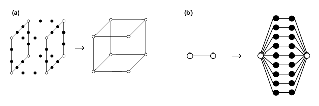
Figure 1: (a) The Migdal-Kadanoff approximate renormalization-group transformation on the cubic lattice. Bonds are removed from the cubic lattice to make the renormalization-group transformation doable. The removed bonds are compensated by adding their effect to the decimated remaining bonds. (b) A hierarchical model is constructed by self-imbedding a graph into each of its bonds, ad infinitum.BerkerOstlund The exact renormalization-group solution proceeds in the reverse direction, by summing over the internal spins shown with the dark circles. Here is the most used, so called ”diamond” hierarchical lattice BerkerOstlund ; Kaufman1 ; Kaufman2 ; BerkerMcKay . The length-rescaling factor $b$ is the number of bonds in the shortest path between the external spins shown with the open circles, $b=3$ in this case. The volume rescaling factor $b^{d}$ is the number of bonds replaced by a single bond, $b^{d}=27$ in this case, so that $d=3$.

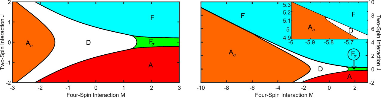
Figure 2: Calculated phase diagram of the XY Ashkin-Teller model. The ferromagnetic $(F)$ and antiferromagnetic $(A)$ phases of the continuously orientable spin variables $\vec{s}_{i}$ and $\vec{t}_{i}$, and the ferromagnetic $(F_{\sigma})$ and antiferromagnetic $(A_{\sigma})$ phases of the composite spin variable $\vec{s}_{i}\vec{t}_{i}$, and the disordered phase $(D)$ are shown. The inset on the right shows the reverse bifurcation where a phase boundary splits into two phase boundaries and one of the latter reverses direction. A similar phenomenon occurs symmetrically at negative $J$.

As part of the first, decimation, step of the renormalization-group transformation, a decimated bond is obtained by integrating over the shared two spins of two bonds. With $u_{ij}(\theta_{ij},\varphi_{ij})=e^{-\beta{\cal H}_{ij}(\vec{s}_{i},\vec{t}_{i};\vec{s}_{j},\vec{t}_{j})}$ being the exponentiated nearest-neighbor Hamiltonian between sites $(i,j)$, and $\theta_{ij}=\theta_{i}-\theta_{j}$ and $\varphi_{ij}=\varphi_{i}-\varphi_{j}$ being the angles between the planar unit vectors $(\vec{s}_{i},\vec{s}_{j})$ and $(\vec{t}_{i},\vec{t}_{j})$, decimation proceeds as

$$\tilde{u}_{13}(\theta_{13},\varphi_{13})=\int_{0}^{2\pi}u_{12}(\theta_{12},\varphi_{12})u_{23}(\theta_{23},\varphi_{23})\frac{d\theta_{2}}{2\pi}\frac{d\varphi_{2}}{2\pi}.$$ (2)

Using the double Fourier transformation Jose ; BerkerNel

$$f(k,l)=\int_{0}^{2\pi}{u(\theta,\varphi)}e^{ik\theta+il\varphi}\frac{d\theta}{2\pi}\frac{d\varphi}{2\pi},\\ u(\theta,\varphi)=\sum_{k=-\infty}^{\infty}\sum_{l=-\infty}^{\infty}e^{-ik\theta-il\varphi}f(k,l),$$ (3)

the decimation of Eq.(2) becomes

$$\tilde{f}_{13}(k,l)=f_{12}(k,l)f_{23}(k,l).$$ (4)

As part of the second, bond-moving, step of the renormalization-group transformation, a bond moving is effected as

$$u_{ij}^{\prime}(\theta,\varphi)=\tilde{u}_{i_{1}j_{1}}(\theta,\varphi)\,\tilde{u}_{i_{2}j_{2}}(\theta,\varphi),\\ f_{ij}^{\prime}(k,l)=\sum_{m=-\infty}^{\infty}\sum_{n=-\infty}^{\infty}\tilde{f}_{i_{1}j_{1}}(k-m,l-n)\tilde{f}_{i_{2}j_{2}}(m,n).$$ (5)

We have followed the renormalization-group flows in terms of the $k=0$ to 20 and $l=0$ to 20 double Fourier components, also using $f_{ij}(k,l)=f_{ij}(-k,l)=f_{ij}(k,-l)=f_{ij}(-k,-l)$. We also made spot checks with higher number of double Fourier components (up to $k,l=0$ to 100). We set to unity the maximum value of the double Fourier components, by dividing with the same constant (the raw maximal value), which amounts to adding the same constant to all energies.

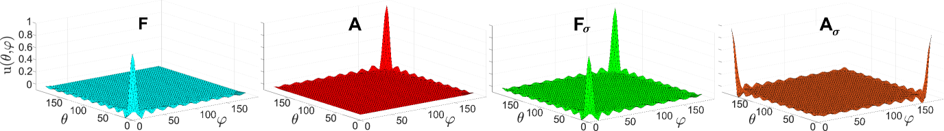
Figure 3: Renormalization-group sinks of the phases of the XY Ashkin-Teller model. The exponentiated nearest-neighbor energy $u_{ij}=e^{-\beta{\cal H}_{ij}(\vec{s}_{i},\vec{t}_{i};\vec{s}_{j},\vec{t}_{j})}$ is shown, as a function of the angle $\theta$ between the spins $\vec{s}_{i},\vec{s}_{j}$ and the angle $\varphi$ between the spins $\vec{t}_{i},\vec{t}_{j}$ . The energies are normalized to the maximum value of $u=1$ by the inclusion of an additive constant to the energy.

III Results: Phase Diagram, Entropic Ordered Phases, Reverse Bifurcation

The phase diagram (Fig. 2) is obtained by following the renormalization-group flows of the double Fourier components, obtained as described above, to their stable fixed points, namely sinks. The basin of attraction of each sink is a corresponding thermodynanic phase.BerkerWor In this XY-Ashkin-Teller model, there are five sinks and therefore five distinct thermodynamic phases. The exponentiated nearest-neighbor interactions, $u_{ij}(\theta_{ij},\varphi_{ij})=e^{-\beta{\cal H}_{ij}(\vec{s}_{i},\vec{t}_{i};\vec{s}_{j},\vec{t}_{j})}$, reconstructed [Eq.(3)] from the double Fourier coefficients, at four of these sinks are shown in Fig. 3. A sink epitomizes the ordering of its corresponding thermodynamic phase that it attracts under renormalization group. Thus, as seen leftmost in Fig. 3, in the ferromagnetic phase $F$, the $\vec{s}_{i}$ spins are aligned $(\theta_{ij}=0)$ with each other and separately the $\vec{t}_{i}$ spins are aligned $(\varphi_{ij}=0)$ with each other. In the antiferromagnetic phase $A$, the neighboring $\vec{s}_{i}$ spins are antialigned $(\theta_{ij}=\pi)$ with each other and separately the neighboring $\vec{t}_{i}$ spins are antialigned $(\varphi_{ij}=\pi)$ with each other. In the entropic composite ferromagnetic phase $F_{\sigma}$, the neighboring spins $\vec{s}_{i}=\pm\vec{s}_{j}$ and simultaneously $\vec{t}_{i}=\pm\vec{t}_{j}$, the upper (or lower) signs being jointly valid, $\theta_{ij},\varphi_{ij}=0$ or $\pi$. In the also entropic composite antiferromagnetic phase, in neighboring $(s_{i},s_{j})$ and $(t_{i},t_{j})$ are either respectively aligned and antialigned, or respectively antialigned and aligned. The latter two ordered phases have an entropy per bond $S/N=\ln 2.$ Furthermore, in all four ordered phases, the relative orientation of the $s_{i}$ and $t_{i}$ systems has a global degeneracy of $2\pi$. The sink of the disordered phase (not shown in Fig. 3) has the (0,0) double Fourier component equal to unity, all other double Fourier components equal to zero. Therefore, $u_{ij}(\theta_{ij},\varphi_{ij})=e^{-\beta{\cal H}_{ij}(\vec{s}_{i},\vec{t}_{i};\vec{s}_{j},\vec{t}_{j})}=1$ independent of angle. Calculated phase diagram exhibits (inset of Fig. 2) a reverse bifurcation where a phase boundary splits into two phase boundaries and one of the latter reverses direction. This phenomenon occurs symmetrically at positive and negative $J$.

IV Conclusion

We have solved, by renormalization-group theory, the Ashkin-Teller type doubled-up XY magnetic spin model in spatial dimension $d=3$. We find four different ordered phases, with ferromagnetic and antiferromagnetic orderings of the direct and composite spins. Two reverse bifurcations, where a phase boundary splits into two phase boundaries and one of the latter reverses directions, occurs symmetrically at positive and negative $J$.

- (1) J. Ashkin and E. Teller, Statistics of Two-Dimensional Lattices with Four Components, Phys. Rev. 64, 178 (1943).
- (2) R. V. Ditzian, J. R. Banavar, G. S. Grest, and L. P. Kadanoff, Phase Diagram for the Ashkin-Teller Model in Three Dimensions, Phys. Rev. B 22, 2542 (1980).
- (3) I. Keçoğlu and A. N. Berker, Global Ashkin–Teller Phase Diagrams in Two and Three dimensions: Multicritical Bifurcation versus Double Tricriticality-Endpoint, Physica A 30, 129248 (2023).
- (4) A. A. Migdal, Phase transitions in gauge and spin lattice systems, Zh. Eksp. Teor. Fiz. 69, 1457 (1975) [Sov. Phys. JETP 42, 743 (1976)].
- (5) L. P. Kadanoff, Notes on Migdal’s recursion formulas, Ann. Phys. (N.Y.) 100, 359 (1976).
- (6) A. N. Berker and S. Ostlund, Renormalisation-group calculations of finite systems: Order parameter and specific heat for epitaxial ordering, J. Phys. C 12, 4961 (1979).
- (7) R. B. Griffiths and M. Kaufman, Spin systems on hierarchical lattices: Introduction and thermodynamic limit, Phys. Rev. B 26, 5022R (1982).
- (8) M. Kaufman and R. B. Griffiths, Spin systems on hierarchical lattices: 2. Some examples of soluble models, Phys. Rev. B 30, 244 (1984).
- (9) A. N. Berker and S. R. McKay, Hierarchical Models and Chaotic Spin Glasses, J. Stat. Phys. 36, 787 (1984).
- (10) R. H. Kraichnan, Dynamics of Nonlinear Stochastic Systems, J. Math. Phys. 2, 124 (1961).
- (11) P. J. Flory, Principles of Polymer Chemistry (Cornell University Press: Ithaca, NY, USA, 1986).
- (12) M. Kaufman, Entropy Driven Phase Transition in Polymer Gels: Mean Field Theory, Entropy 20, 501 (2018).
- (13) P. Lloyd and J. Oglesby, Analytic Approximations for Disordered Systems, J. Phys. C: Solid St. Phys. 9, 4383 (1976).
- (14) E. C. Artun, D. Sarman, and A. N. Berker, Nematic Phase of the n-Component Cubic-Spin Spin Glass in d=3: Liquid-Crystal Phase in a Dirty Magnet, Physica A 40, 129709 (2024).
- (15) Y. E. Pektaş, E. C. Artun, and A. N. Berker, Driven and Non-Driven Surface Chaos in Spin-Glass Sponges, Chaos, Solitons and Fractals 17, 114159 (2023).
- (16) J. Clark and C. Lochridge, Weak-disorder limit for directed polymers on critical hierarchical graphs with vertex disorder, Stochastic Processes Applications 158, 75 (2023).
- (17) M. Kotorowicz and Y. Kozitsky, Phase transitions in the Ising model on a hierarchical random graph based on the triangle, J. Phys. A 55,405002 (2022).
- (18) P. P. Zhang, Z. Y. Gao, Y. L. Xu, C. Y. Wang, and X. M. Kong, Phase diagrams, quantum correlations and critical phenomena of antiferromagnetic Heisenberg model on diamond-type hierarchical lattices, Quantum Science Technology 7, 025024 (2022).
- (19) K. Jiang, J. Qiao, and Y. Lan, Chaotic Renormalization Flow in the Potts model induced by long-range competition, Phys. Rev. E 103, 062117 (2021).
- (20) G. Mograby, M. Derevyagin, G. V. Dunne, and A. Teplyaev, Spectra of perfect state transfer Hamiltonians on fractal-like graphs, J. Phys. A 54, 125301 (2021).
- (21) I. Chio, R. K. W. Roeder, Chromatic zeros on hierarchical lattices and equidistribution on parameter space, Annales de l’Institut Henri Poincaré D, 8, 491 (2021).
- (22) B. Steinhurst and A. Teplyaev, Spectral analysis on Barlow and Evans’ projective limit fractals, J. Spectr. Theory 11, 91 (2021).
- (23) A. V. Myshlyavtsev, M. D. Myshlyavtseva, and S. S. Akimenko, Classical lattice models with single-node interactions on hierarchical lattices: The two-layer Ising model, Physica A 558, 124919 (2020).
- (24) M. Derevyagin, G. V. Dunne, G. Mograby, and A. Teplyaev, Perfect quantum state transfer on diamond fractal graphs, Quantum Information Processing, 19, 328 (2020).
- (25) S.-C. Chang, R. K. W. Roeder, and R. Shrock, q-Plane zeros of the Potts partition function on diamond hierarchical graphs, J. Math. Phys. 61, 073301 (2020).
- (26) C. Monthus, Real-space renormalization for disordered systems at the level of large deviations, J. Stat. Mech. - Theory and Experiment, 013301 (2020).
- (27) O. S. Sarıyer, Two-dimensional quantum-spin-1/2 XXZ magnet in zero magnetic field: Global thermodynamics from renormalisation group theory, Philos. Mag. 99, 1787 (2019).
- (28) J. V. José, L. P. Kadanoff, S. Kirkpatrick, and D. R. Nelson, Renormalization, vortices, and symmetry-breaking perturbations in two-dimensional planar model, Phys. Rev. B 16, 1217 (1977).
- (29) A. N. Berker and D. R. Nelson, Superfluidity and Phase Separation in Helium Films, Phys. Rev. B 19, 2488 (1979).
- (30) A. N. Berker and M. Wortis, Blume-Emery-Griffiths-Potts Model in Two Dimensions: Phase Diagram and Critical Properties from a Position-Space Renormalization Group, Phys. Rev. B 14, 4946 (1976).