A high-fidelity surrogate model for the ion temperature gradient (ITG) instability using a small expensive simulation dataset

Abstract

One of the main challenges in building high-fidelity surrogate models of tokamak turbulence is the substantial demand for high-quality data. Typically, producing high-quality data involves simulating complex physical processes, which requires extensive computing resources. In this work, we propose a fine tuning-based approach to develop the surrogate model that reduces the amount of high-quality data required by 80%. We demonstrate the effectiveness of this approach by constructing a proof-of-principle ITG surrogate model using datasets generated from two gyrokinetic codes, GKW and GX. GX needs in terms of computing resources are much lighter than GKW. Remarkably, the surrogate models’ performance remain nearly the same whether trained on 798 GKW results alone or 159 GKW results plus an additional 11979 GX results. These encouraging outcomes indicate that fine tuning methods can significantly decrease the high-quality data needed to develop the simulation-driven surrogate model. Moreover, the approach presented here has the potential to facilitate surrogate model development for heavy codes and may ultimately pave the way for digital twin systems of tokamaks.

Keywords: surrogate model, fine-tune, turbulence, gyrokinetic

1 Introduction

Predicting the temperature and density of the core plasma in tokamaks is crucial for optimizing discharge scenarios, interpreting fusion experiments, and designing future fusion devices. Typically, time-evolved simulations of tokamak discharges over the course of a pulse are performed using an "integrated modeling" approach , such as ETS [1], PTRANSP [2], TSC [3], TRANSP [4], CRONOS [5], JINTRAC [6], METIS [7], ASTRA [8], TOPICS [9], etc. These approaches integrate multiple module codes, each addressing a different physical process in tokamak plasmas, into a single workflow. A key component of these integrated models is the prediction of turbulent fluxes, particularly in the core of the tokamak, where plasma microinstabilities often dominate transport. However, calculating these fluxes using nonlinear gyrokinetic models is computationally demanding for routine simulation of tokamak discharge evolution.

The plasma physics community has developed numerous first-principles or empirical physics codes to address these challenges under varying fidelity conditions. Gradient-driven codes include GENE [10], GKW [11], GS2 [12], GX [13], and GYRO [14]. In addition, there are flux-driven codes such as GYSELA [15] and GT5D [16]. Some physical-point-acceleration codes include QuaLiKiz [17, 18] and TGLF [19]. These simulation codes are effective, but there is always a trade-off between physical fidelity and computational efficiency. Basically, high physical fidelity often makes simulations computationally expensive for routine tokamak simulations and vice versa. However, scenarios such as uncertainty quantification, scenario optimization, and controller design demand fast, high-fidelity simulation codes, particularly for many-query applications like multi-dimensional integrated models (e.g., [20, 21, 7, 6]), where both speed and accuracy are paramount.

Recently, the machine learning (ML) method has emerged as a powerful alternative for new model development by learning from simulation or experimental datasets, often referred to as surrogate models. ML surrogate models can capture the complex relationships between plasma parameters and tokamak response. To date, many surrogate models based on neural networks have been developed to solve different tasks in tokamaks, such as tokamak operation [22], integrated modeling [23] etc. Based on the data type usage, these surrogate,models can be divided into two categories: experimental data-driven and simulation data-driven models.

Experimental data-driven surrogate models have achieved significant advancements, including disruption prediction [24, 25], tokamak operation based on reinforcement learning [26, 27], last closed-flux surface reconstruction [28, 29], entire discharge estimation [30, 31]. These methods are accurate and capable of reconstructing the discharge process of an operating tokamak based on input parameters. However, experimental data-driven models face challenges in interpreting experimental results due to the lack of theoretical models. Furthermore, it seems impractical to directly apply them to the design or operation of new devices.

Simulation data-driven surrogate models run efficiently and have the capability to explain physical processes in tokamak experiments, as well as aid in designing new tokamak devices. Due to these advantages, simulation data-driven surrogate models have been receiving increasing attention. Several efforts have been made in this area, including the quasilinear turbulent transport codes, TGLF ($\sim 2$ CPUs per case) [32, 19, 33] and QualiKiz ($\sim 30$ CPUs per case) [17, 33], the pedestal confinement code EPED ($\sim 10$ CPUh per case) [32, 19], the neutral beam heating code NUBEAM ($\sim 1$ CPUh per case) [34, 35, 23], and the tokamak edge plasma code SOLPS, which can take months of wall-clock time for high-fidelity simulations [36, 37]. Successful simulation-driven surrogate model typically fall into two categories: (1) fast-running models like TGLF, QualiKiz, EPED, and NUBEAM, which can efficiently generate large datasets, or (2) models such as SOLPS-ITER, where extensive datasets are already available. However, developing high-fidelity nonlinear simulation-driven surrogate models from scratch presents significant challenges due to the prohibitive computational cost of generating large training datasets. For instance, a simple ITG case using GKW requires $\sim 300$ CPU hours, while developing a typical 4D surrogate model like QLKNN-4D [38] generally needs $\sim 10^{6}$ cases. Acquiring such a large amount of high-fidelity data is often either infeasible or highly resource-intensive.

The computational cost of nonlinear gyrokinetic simulation codes is typically high, making it an urgent challenge to build a surrogate model with a small dataset. Developing surrogate models for gyrokinetic simulation codes using a sizable, high-fidelity nonlinear dataset is practically infeasible. Several innovative approaches have been explored to address this issue. These include adaptive sampling training database [39], hybrid machine learning and physical simulations to reduce the data requirements [40], physics-constrained neural networks [41], Generative Artificial Intelligence (GAI) [42], and neural partial differential equation (PDE) surrogates [43]. These methods incorporate physical prior knowledge to varying degrees, effectively reducing the data requirements for high-fidelity surrogate models. However, to the best of the authors’ knowledge, few studies [44] have explored leveraging large amounts of low-fidelity data to enhance the performance of surrogate models on the high-fidelity data.

In this work, we aim to address this problem by introducing a novel surrogate model-building approach as a proof of concept. We begin by generating a sizable dataset of low-fidelity, rapid simulations using fast codes with low resolution, followed by a smaller dataset of high-fidelity, high-resolution simulations to refine the model. This strategy strikes a balance between precision and computational efficiency, enabling the development of effective gyrokinetic surrogate models. Specifically, we are focusing on constructing a surrogate model for ion thermal diffusivity $\chi_{i}$ and wave number spectrum of ITG modes using GKW [11] and GX [13].

All simulations are run with 1 ion species (D) and adiabatic electrons with scanning four parameter inputs: safety factor $q$, magnetic shear $\hat{s}$, ion temperature gradient $R/L_{T_{i}}$, and density gradient $R/L_{n}$. The outputs are ion thermal diffusivity $\chi_{i}$ and wave number spectrum. We collected 13310 simulation results using the GX code to primarily train our machine learning (ML) model and generated 1267 high-fidelity results using the GKW code to fine-tune and validate the model’s accuracy.

The surrogate model, developed with only 159 GKW results and 11979 GX results, achieved the same performance as a model trained with 798 GKW results alone. This approach reduced the requirement for high-resolution, computationally expensive results by 80% while maintaining equivalent accuracy. Furthermore, the surrogate model, based on a neural network, is orders of magnitude faster than direct simulations, requiring only approximately one milliseconds per case, making it suitable for real-time modeling.

The present paper is structured as follows. Section 2 details the dataset preparation, the methodology for constructing the machine learning model, and the training procedures. Section 3 highlights the performance of the surrogate model, including a comparative analysis with other models. Finally, Section 4 provides a brief discussion and conclusion.

2 Methods

In this section, we provide detailed explanations of the dataset, machine learning model construction, and model training process.

2.1 Dataset generation

To generate a database for ITG instabilitiy, nonlinear gyrokinetic simulations are performed using both GKW and GX codes. GKW [11] is a CPU-based code that solves turbulent transport problems on a fixed grid in five-dimensional space, employing a combination of finite difference and pseudo-spectral methods. It utilizes Fourier pseudo-spectral techniques in spatial dimensions and is a high-fidelity and computationally intensive code. In our ITG instability simulations, each GKW case required approximately 300 CPU hours. GX [13] is a GPU-native code designed for solving the nonlinear gyrokinetic system governing low-frequency turbulence in magnetized plasmas, including those in tokamaks and stellarators. It employs a Fourier-Laguerre-Hermite pseudo-spectral formulation in phase space, offering a fast gyrokinetic solver that requires only $\sim 0.25$ GPU hours per case for our ITG instability simulations. While GX and GKW provide comparable fidelity, we adjusted the resolution in velocity space for GX and slightly modified other parameters that lower the fidelity of the resulting simulation compared with our GKW cases. (see table 1). All other settings were kept consistent with those used in GKW, such as flux surface geometry of Miller equilibrium, elongation of flux surface equal to 1, collision frequency to 0, etc. Notably, when GX was configured to closely match GKW, our test case indicated that GX required $\sim 12$ GPU hours per case.

Table 1: The difference between GKW and GX in our simulation.

	GKW	GX
Architecture	CPU-based	GPU-based
Spectral method in space	Fourier Pseudo-spectral in space	Fourier Laguerre Hermite pseudo spectral formulation in phase space
Speed per case	$\sim\boldsymbol{300}$ CPU hours	$\sim\boldsymbol{0.25}$ GPU hours
Parallel $V_{\parallel}$ mesh points	64	8
$\mu$ mesh points	8	4
Max. time steps	1200	400

The input space of GX and GKW codes ( $\sim 15$ dimensions for typical simulations) is too large with brute-force scans, especially for a demonstrative proof-of-principle study. Therefore, we reduced the input parameter space to a subset that significantly impacts our goal: the ITG mode. The selected input parameters and their ranges, shown in table 2, include the ion temperature gradient ($R/L_{T_{i}}$), density gradient ($R/L_{n}$), safety factor ($q$), magnetic shear ($\hat{s}$).

The dataset comprises 1267 GKW and 13310 GX simulations. The simulations required approximately 0.39 million CPU hours (MCPUh) and 0.33 million GPU hours (MGPUh). The input space was structured as a rectangular, uniform four-dimensional grid, with bounds covering the parameter regimes typically encountered in the core of standard aspect-ratio present-day tokamaks and future devices such as ITER and DEMO. The dataset, stored in HDF5 format, occupies approximately 4 GB of storage.

Table 2: 4D hyperrectangle bounds and number of points of the GX and GKW dataset. Each input parameter is uniformly distributed to widely verify our methodology.

Variable	GKW points	GX points	Min	Max
Ion temperature gradient, $R/L_{T_{i}}$	6	11	4.5	7
Density gradient,$R/L_{n}$	6	11	0.5	3.0
Safety factor, $q$	6	11	1	3
Magnetic shear, $\hat{s}$	6	10	0.1	1
GKW valid calculations	1267	-	$\approx$ 0.39 MCPUh
GX valid calculations	-	13310	$\approx$ 0.33 kGPUh

2.2 Data preprocessing

Once the data is generated, we preprocess the datasets to extract key information and restructure them to ensure compatibility with the machine learning models. The data preprocessing workflow can be divided into three steps: data cleaning, reduction, and splitting.

2.2.1 Data cleaning

Gyrokinetic nonlinear simulations are inherently complex and numerically challenging, requiring intricate setups and often encountering numerical instabilities introduced by nonlinearities in the model. Some simulations may fail or not converge. In this paper, we apply three simple criteria to determine the validity of our simulations:

1. The total simulation steps exceeds 600 for GKW, and 200 for GX.

2. The simulation reaches nonlinear saturation beginning at or before 60% of the total simulation duration.

3. The $k_{x}$ spectrum $\phi_{x}$ and $k_{y}$ spectrum $\phi_{y}$ have over 20 points and 10 points in the ranges of $[-1.6,1.6]$ and $[0,0.75]$, respectively. These ranges are determined by the wavenumbers that researchers are interested in and the significant linear growth rate spans [45].

A simulation is considered invalid if it terminates too early, as this typically indicates numerical instability or computational failure. Additionally, if the nonlinear saturation phase is too short, averaging quantities $\chi_{i}$, $\phi_{x}$, $\phi_{y}$ will be inaccurate, over the final 40% of the simulation length may lead to inaccurate results. Finally, if the number of points in the wavenumber intervals predicted by the machine learning model is insufficient, the surrogate model’s accuracy and reliability will be significantly affected. Notably, the intervals [-1.6, 1.6] of $k_{x}$, and [0, 0.75] of $k_{y}$ is a choice to balance the computational resource and physical requirements. If the $k_{x}$, and $k_{y}$ regime is excessively broad, the computational resource requirements increase significantly. Because in order to simplify the surrogate model, we fixed the dimensionality of the output. The representative case in this context is the cyclone case. In this case, for the toroidal mode number relevant to ITG, $k_{y}$ corresponds to approximately 0.5. As shown in [45], the region exhibiting a significant linear growth rate spans from 0 to 0.7. Hence, we set the range of $k_{y}$ from 0 to 0.75.

2.2.2 Data reduction

The raw simulation data from GKW and GX consists of time sequences, with sequence lengths depending on the simulation time steps. In this study of ITG simulations, we focus only on the final effects of the wave spectrum and thermal diffusivity. First, we calculate the average values of $\chi_{i}$, $\phi_{x}$, and $\phi_{y}$ over the last 40% of the simulation time steps. Next, we apply linear interpolation to $\phi_{x}$ and $\phi_{y}$ to align these values. After interpolation, $\phi_{x}$ and $\phi_{y}$ contain 101 and 51 points, respectively, covering $k_{x}$ and $k_{y}$ the ranges of [-1.6, 1.6] and [0, 0.75]. Finally, we take the logarithmic scale of $\phi_{x}$, and $\phi_{y}$ . With these processing steps, the target of our model will have 153 channels: 1 channel for $\chi_{i}$, 101 channels for $\phi_{x}$, and 51 channels for $\phi_{y}$.

2.2.3 Data splitting

In this paper, we use two code GKW and GX simulation results. Firstly, we randomly split the GKW dataset into three subsets: $S_{1}$ , $S_{2}$, and $S_{3}$, containing 63%, 7%, and 30% of the data, which correspond to 798, 89, and 380 GKW simulation results, respectively. Next, we randomly divide the GX simulation dataset into $S_{4}$ and $S_{5}$ with proportions of 90% and 10%, encompassing 11979 and 1331 GX simulation results, respectively. Notably, $S_{3}$ is a slightly larger test set proportion compared to those typically used in machine learning studies, as we aim to evaluate our method across a broader parameter space using a extensive dataset.

2.3 Machine learning model

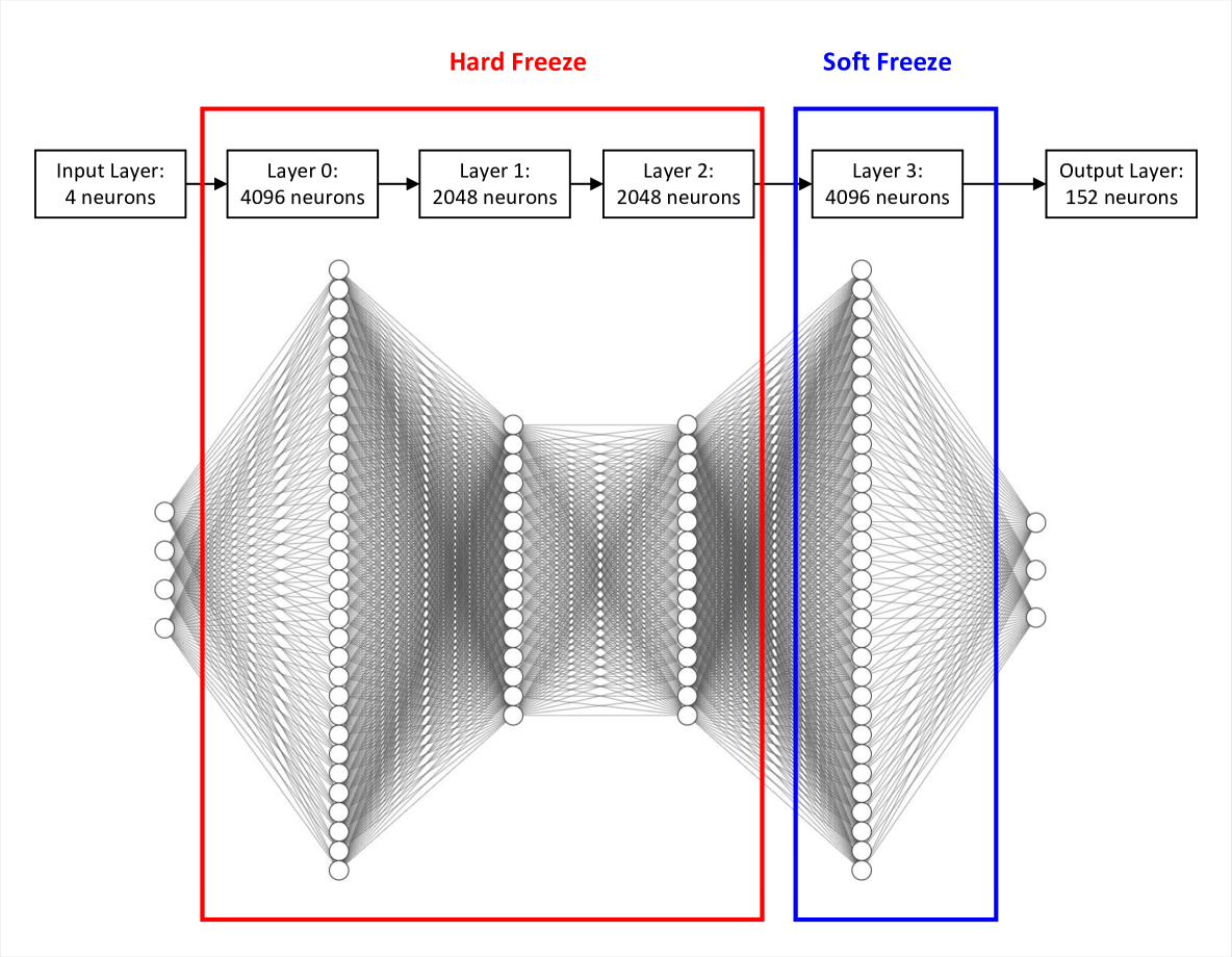
Figure 1: Fine-tuning technology in our MLP model. The red box is defined with a zero learning rate, while the blux box, labeled "Soft freeze", is set to a learning rate of $1\times 10^{-5}$.

Recently, the remarkable success of generative artificial intelligence applications like Chat-GPT [46, 47] and Stable Diffusion [48] has highlighted the effectiveness of fine-tuning. Fine-tuning involves leveraging knowledge from a large, low-accuracy dataset and refining it with a smaller, high-accuracy dataset to enhance model performance for a specific task. As illustrated in figure 1, for the fine-tuned model, we apply a similar fine-tuning approach to train a gyrokinetic surrogate model, utilizing fast, low-resolution simulation data to improve the model’s performance on high-resolution, low-speed simulations. Specifically, for fine-tuning, we follow these steps:

1. Initial Training: Train the entire neural network using $S_{4}$ and $S_{5}$ as the training and validation sets with a learning rate of $1\times 10^{-3}$

2. Model Selection: Select the best-performing model based on validation set performance.

3. Layer Freezing: Apply a “hard freeze” to the first three layers (setting their learning rate to 0) and a “soft freeze” to the last layer (setting its learning rate to $5\times 10^{-5}$).

4. Re-training: Re-train the neural network using 20% $S_{1}$ and 20% $S_{2}$ as training and validation sets.

5. Testing: Test the model on set $S_{3}$.

For the GX-only and the GKW-only simulation result training models, we do something similar, but only use steps 1, 2, and 5. And in the GKW simulation trained model, in step 1 we use $S_{1}$, $S_{2}$ instead of $S_{4}$, $S_{5}$.

In our approach, the “hard freeze” (learning rate of 0) prevents specific layers from being modified by the model trained with the new data, while the “soft freeze” (learning rate of $1\times 10^{-5}$) allows limited adjustments to align the model with new data. In our case, the new data refers to GKW simulation results. This strategy assumes that the earlier layers capture general lower-level knowledge suitable for gyrokinetic ITG simulations, whereas the later layers are more likely to discern high-level knowledge relevant to the specific task for which the model is being trained.

Table 3: The loss comparison among multiple models. The MLP is the simplest neural network model. The CNN is a convolution-based model commonly used in image processing. Transformer and Transformer Encoder are attention-based models widely used in large language model applications. Based on the MSE loss comparison, the MLP model achieved the best performance.

Model type	Mean Squared Error (MSE) loss
Multilayer perceptron (MLP)	$\sim 1\times 10^{-4}$
Transformer	$\sim 1\times 10^{-2}$
Transformer Encoder	$\sim 1\times 10^{-2}$
Convolutional Neural Networks (CNN)	$\sim 1\times 10^{-3}$

In this paper, we compare the training results of the MLP model with three other popular models: CNN, Transformer, and Transformer Encoder on GX data, all of which have the same parameter size of $\sim 10$ million. MLP (Multilayer Perceptron): This is the simplest type of neural network, consisting of fully connected layers. Its advantages include ease of implementation and interpretability, making it suitable for problems with structured numerical data. However, it may struggle to capture spatial structures or long-range dependencies. CNN (Convolutional Neural Network): This model leverages convolution operations and is commonly used in image processing tasks. It is effective at capturing local spatial features and has translation invariance, making it useful when data has spatial or local correlations. However, it can require careful design to handle non-spatial or sequential data efficiently. Transformer and Transformer Encoder: These are attention-based models widely used in large language models and sequence modeling tasks. Their main advantage is their ability to capture long-range dependencies and context within data effectively. However, they typically require substantial data and computational resources, and can be more complex to train compared to simpler architectures. Table 3 shows that MLP has the lowest MSE loss value. Generally, in machine learning model evaluation, the smaller the loss value, the better performance of the model. Therefore, we choose MLP for the present work. This choice is also intuitive, as this study serves as a proof-of-principle with only four input parameters (4 channels) and three output parameters (153 channels, with $\chi_{i}$, $\phi_{x}$, and $\phi_{y}$ having 1, 101, and 51 channels, respectively), making their mapping relationship relatively straightforward. More complex, advanced models tend to be harder to converge and typically require larger datasets for effective training.

Our machine learning model was developed using PyTorch on Red Hat Enterprise Linux 8, running on four A100 GPUs. During model training, we utilized the Tree-structured Parzen Estimator (TPE) algorithm [49] to perform the architectural hyperparameter search. Additionally, we experimented with various optimizers and regularization techniques, ultimately identifying the optimal set of hyperparameters, as shown in table 4.

Table 4: Our model hyperparameters. Model architecture can be found in figure 1

Hyperparameter	Explanation	Best value
$\text{$\eta$}_{t}$	Learning rate in model train phase	$1\text{$\times 10^{-3}$}$
$\text{$\eta$}_{f}$	Learning rate in model fine tuning phase	$5\times 10^{-4}$
$\text{Epoch}_{t}$	Number of epochs in model train	800
$\text{Epoch}_{f}$	Number of epochs in model fine tuning phase	1000
Optimizer	Optimizer type	Stochastic Gradient Descent (SGD)
Loss	Loss function	Mean Squared Error (MSE) loss
Scheduler	Scheduler type	OneCycle[50]
Dropout	Dropout probability	0.1
$B$	Batch size	4
$C_{i}$	Input channels	4
$C_{o}$	Output channels	152
$E_{\text{mlp}}$	Embed layers	[4096, 2048, 2048, 4096]

3 Results

After completing the model training, we obtained three models: the GKW-trained model, the GX-trained model, and the fine-tuned model. To evaluate the quality of these neural networks and assess the impact of our underlying assumptions, we compared them with the actual GKW simulation results for $\chi_{i}$ versus $R/L_{T}$ with $q=1.4$, $\hat{s}=0.64$ in figure 2. The figure illustrates that the GX trained model does not align well with the real GKW labels, whereas the GKW-trained model closely matches them. Despite employing multiple techniques to prevent overfitting, the GKW trained model’s fit is almost too perfect, raising some concerns about potential overfitting. In contrast, while the fine-tuned model is not as precise as the GKW-trained model, it produces smoother curves in the $\chi_{i}$ vs. $R/L_{T}$ plot, particularly in regions far from the turbulence threshold. It is important to note that the non-monotonic behavior of $\chi_{i}$ near the threshold may pose challenges for integrated modeling, as abrupt variations in transport coefficients can compromise numerical stability and convergence. Since this study serves as a proof of concept, we prioritize clarity and ease of understanding in our methodology. However, to mitigate this issue in future work, we will explore: (1) Threshold labeling based on extensive simulation cases. (2) As shown in [51], training a classifier to identify the threshold, and (3) Restricting regression model training to the monotonic region above the threshold. These improvements will enhance the monotonicity of the surrogate model.

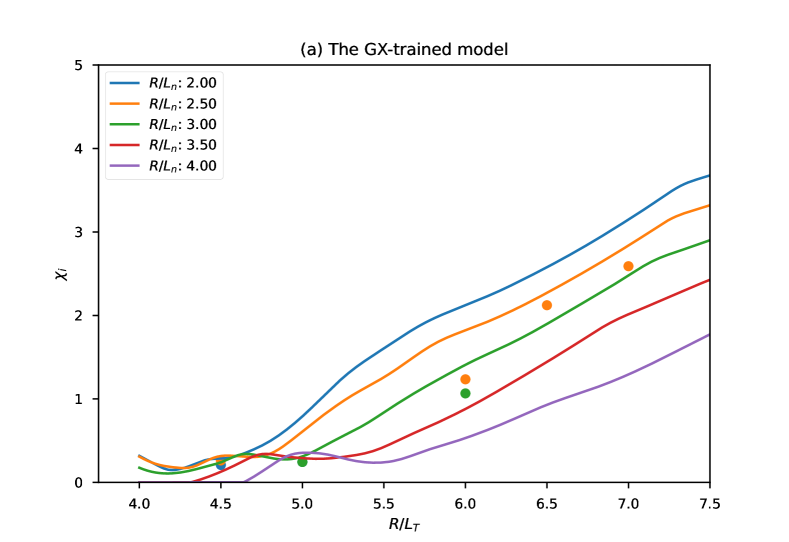
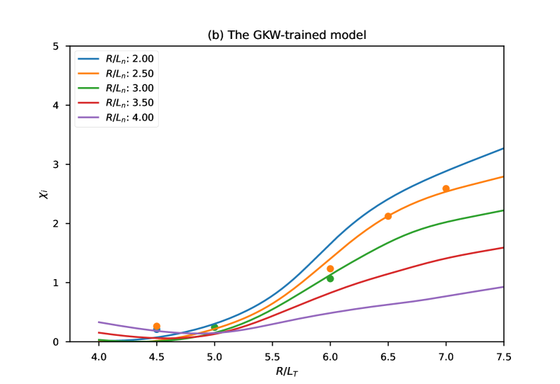
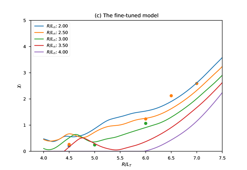
Figure 2: The plots of $\chi_{i}$ versus $R/L_{T}$ with $q=1.4,$ $\hat{s}=0.64$. The solid lines $\chi_{i}$ vs. $R/L_{T}$ for different $R/L_{n}$. All circular points in three subplots indicate actual GKW simulation results, with colors corresponding to the $R/L_{n}$ values of the solid lines. The behavior below the threshold (i.e. non-zero flux below the threshold) will be problematic for any integrated modeling application, making surrogate models inaccurate in this region.

Figure 3 presents a comparison of the two models, both the GKW-trained and fine-tuned models, with typical GKW and corresponding GX simulations, illustrating the $k_{x}$ spectrum $\phi_{x}$ and the $k_{y}$ spectrum $\phi_{y}$. The fine-tuned and GKW-trained models exhibit almost identical performance when the $k_{x}$ wavenumber exceeds 0.25 or the $k_{y}$ wavenumber exceeds 0.1. In the zoom in subplot of figure 3, at low $k_{x}$ wavenumbers, the fine-tuned model closely fits the GX simulation represented by the black crossed solid line. This may explain why the fine-tuned model overestimates $\phi_{x}$ in low $k_{x}$ wavenumbers. Overall, the $\phi_{y}$ predictions from both surrogate models align well with the actual GKW simulations across the entire range of $k_{y}$ wavenumbers. In detail, the fine-tuned model performs slightly worse than the GKW-trained model at low wavenumbers. The challenge arises because the GKW and GX simulations do not have densely sampled data points at low wavenumbers. We plan to address this issue in future studies by performing additional simulations with denser data sampling in the low wavenumber range.

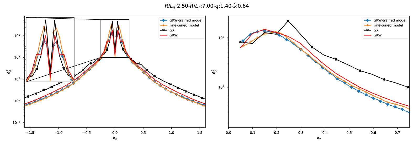
Figure 3: The $\phi_{x}$ and $\phi_{y}$ plots for GKW-trained model, fine-tuned model, actual simulations of GKW and GX. The blue diamonded solid line and the orange starred solid line represent the predicted results of the GKW-trained and fine-tuned models, respectively. The black crossed solid line and the red solid line correspond to the actual simulations of GX and GKW, respectively.

Only one typical result is insufficient to quantitatively evaluate the accuracy of the model. Therefore, the entire test set $S_{3}$ is used to quantify the accuracy of the surrogate models. Figures 4, 5 and 6 show the performance of our models on the entire test set. $R^{2}$ is coefficient of determination; The definition of similarity is as shown in equation 1,

$$S\left(x,y\right) = \frac{\Sigma(\boldsymbol{x}-\bar{\boldsymbol{x}})(\boldsymbol{y}-\bar{\boldsymbol{y}})}{\sqrt{\Sigma(\boldsymbol{x}-\bar{\boldsymbol{x}})^{2}\Sigma(\boldsymbol{y}-\bar{\boldsymbol{y}})^{2}}}$$

similiarity $$= \frac{S\text{$\left(\hat{\phi_{x}},\phi_{x}\right)$}l_{k_{x}}+S\text{$\left(\hat{\phi_{y}},\phi_{y}\right)$}l_{k_{y}}}{l_{k_{x}}+l_{k_{y}}}$$ (1)

where $x$ and $y$ are unknown variables, and $\bar{x}$, $\bar{y}$ are their averages. $l_{k_{x}}$, $l_{k_{y}}$ represent the number of points in $\phi_{x}$ and $\phi_{y}$, respectively, and $S\left(\boldsymbol{x},\boldsymbol{y}\right)$ denotes the Pearson correlation coefficient. This equation uses point normalization to avoid bias in the results due to the differing numbers of points in $\phi_{x}$ and $\phi_{y}$. $\phi_{x}$ and $\hat{\phi_{x}}$ are the target and predicted $k_{x}$ spectrum, and the the same notation applies for $\phi_{y}$ and $\hat{\phi_{y}}$.

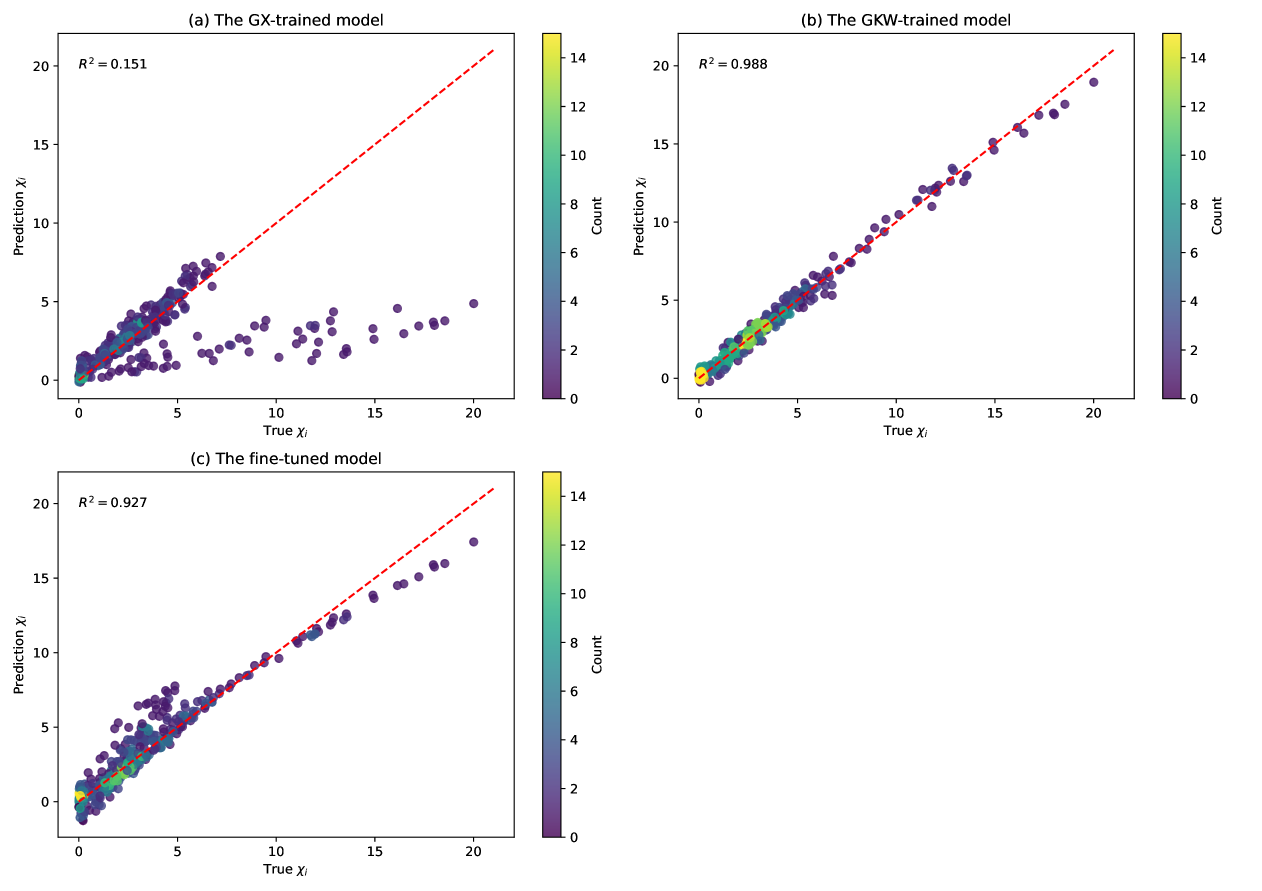
Figure 4: Regression plots of $\chi_{i}$ for the three models. The plots show that GX performs the worst, particularly when $\chi_{i}$ is large. Fine-tuning significantly enhances GX’s performance, making points with small $\chi_{i}$ more concentrated along the diagonal and those with large $\chi_{i}$ closer to it.

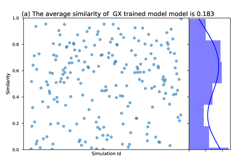
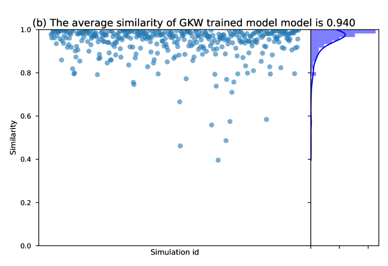
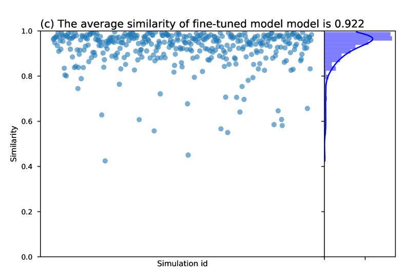
Figure 5: The similarity distribution in the whole test set of (a) GX-trained, (b) GKW-trained, (c) fine-tuned model predictions. The similarity defined as equation 1. To the right of each subfigure are the histograms with density estimates.

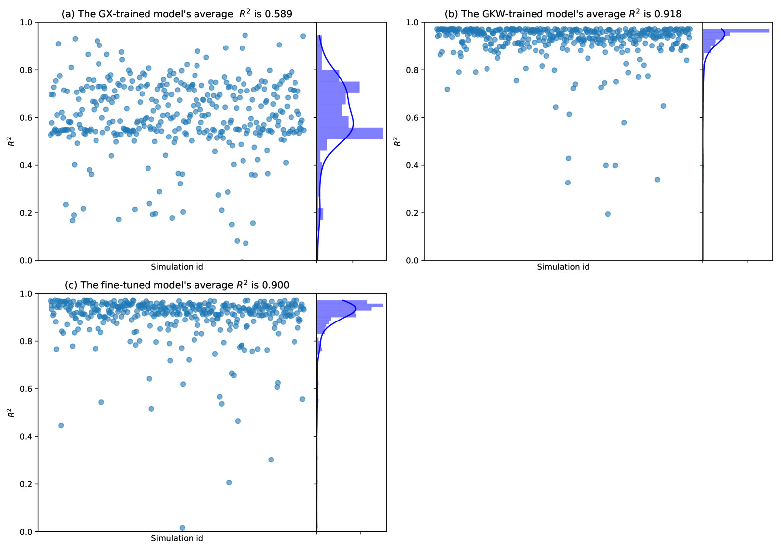
Figure 6: The $R^{2.pdf}$ distribution in the whole test of (a) (a) GX-trained, (b) GKW-trained, (c) fine-tuned model predictions.

From figures 5 and 6, which illustrate the similarity distribution on the test set, we observe that the performance of the model trained with GKW is nearly identical to that of the fine-tuned model. In contrast, the results of the model trained with GX differ significantly from the actual GKW simulations. This indicates that fine-tuning effectively integrates knowledge from both GKW and GX results. From figure 4, we can observe that the fine-tuning model prediction is closer to the diagonal than the GX-trained model prediction, particularly near $\chi_{i}=5$, where the improvement is most noticeable. However, when $\chi_{i}$exceeds 10, the improvement is not satisfactory, likely due to the sparsity of the fine-tune model’s tuning set (20% $S_{1}$).Actually, the fine-tuned model training set $20\%S_{1}$ is different from$S_{3},$ but they are independent and identically distributed. Figure 4(a) shows that the predictions of the GX trained model for $\chi_{i}$ exhibit a subset with notably poor performance below the diagonal. Upon inspection, we find that over 90% of these points correspond to cases with $\hat{s}=0.1$. As discussed by [52, 13], the standard twist-shift boundary condition quantizes the perpendicular aspect ratio as $L_{x}/L_{y}=J/(2\pi|\hat{s}|),$ making resolution particularly demanding for low-shear cases. Although the generalized twist-shift boundary condition provides some flexibility in aspect ratio selection, maintaining numerical accuracy at $\hat{s}\ll 1$remains challenging. As a result, the GX-trained model exhibits a significant discrepancy from the target GKW results in the low-$\hat{s}$ regime. Also, we examine all similarities lower than 0.8 in figures 5(b), 5(c), and all$R^{2}$ values lower than 0.8 in 6(b) and 6(c). The main cases arise from incorrect simulations, such as the $\phi_{x}$ spectrum not being strictly symmetrical. The similarity and $R^{2}$ distributions of the GKW-trained model are more concentrated than that of the fine-tuned model. We believe that this is because the fine-tuning used sparser GKW simulation results than the GKW-trained model. In the future, this could be improved using more appropriate sampling methods, such as adaptive sampling, which can sample more points on challenging results.

4 Discussion and Conclusion

This study demonstrates new possibilities for developing high-fidelity surrogate models for tokamak simulation codes. In the development of the ITG surrogate model, by leveraging a large low-fidelity GX simulation dataset and a small high-fidelity GKW simulation dataset, we achieve comparable accuracy to the model trained exclusively on a large high-fidelity GKW simulation dataset while reducing the need for computationally expensive data by 80%. The comparison between fine-tuned model predictions and actual GKW simulations for thermal diffusivity and wave spectrum was in qualitative agreement. This approach significantly lowers the barriers to developing surrogate models for computationally demanding simulations.

Despite these promising results, the study is still a proof-of-principal work, that warrants further exploration. First, the surrogate model was trained within a relatively limited parameter space, focusing on ion temperature gradient (ITG) modes with four input parameters. Future work should consider expanding this parameter space to include additional physical phenomena such as trapped electron modes (TEM) and electron temperature gradient (ETG) modes. Second, it is necessary to explore more parameters. As noted in this paper, typical gyrokinetic code simulations require $\sim 15$ dimensions of input, and a broader range of parameters should be scanned in future datasets. Additionally, while fine-tuning combines datasets of varying fidelity, the results may be influenced by the specific characteristics of the simulation codes utilized. Further validation across different simulation frameworks or experimental datasets would enhance the generalizability of this method.

The fine-tuning process in this study assumed that low-fidelity GX simulations capture general patterns, while high-fidelity GKW simulations refine these patterns. However, the observed overestimation of wave spectrum in low wavenumber and the underestimation of high $\chi_{i}$ in the fine-tuned surrogate model suggests opportunities to incorporate adaptive sampling techniques, which dynamically select training points to cover challenging regions of the parameter space more effectively. For the thermal diffusivity estimation, we can develop a machine learning–based classification model to categorize parameters as below or above the threshold, and then train the regressive surrogate model on parameters above the threshold. These techniques could further improve model performance and efficiency.

Finally, the approach outlined here aligns with broader efforts to develop digital twin systems for tokamaks [53]. Such systems require fast, accurate, and high-fidelity simulations to predict plasma behavior and optimize operational scenarios in real-time. The fine tuning-based surrogate model provides a foundational framework for achieving these ambitious goals.

Data availability statement

The data that supports the findings of this study belongs to the Singapore SAFE team and is available from the corresponding author upon reasonable request.

References

- [1] G.L. Falchetto, David Coster, Rui Coelho, B.D. Scott, Lorenzo Figini, Denis Kalupin, Eric Nardon, Silvana Nowak, L.L. Alves, J.F. Artaud, V. Basiuk, João P.S. Bizarro, C. Boulbe, A. Dinklage, D. Farina, B. Faugeras, J. Ferreira, A. Figueiredo, Ph. Huynh, F. Imbeaux, I. Ivanova-Stanik, T. Jonsson, H.-J. Klingshirn, C. Konz, A. Kus, N.B. Marushchenko, G. Pereverzev, M. Owsiak, E. Poli, Y. Peysson, R. Reimer, J. Signoret, O. Sauter, R. Stankiewicz, P. Strand, I. Voitsekhovitch, E. Westerhof, T. Zok, and W. Zwingmann. The European Integrated Tokamak Modelling (ITM) effort: Achievements and first physics results. Nuclear Fusion, 54(4):043018, April 2014.
- [2] R V Budny, R Andre, G Bateman, F Halpern, C E Kessel, A Kritz, and D McCune. Predictions of {H}-mode performance in {ITER}. Nuclear Fusion, 48(7):75005, 2008.
- [3] C E Kessel, R E Bell, M G Bell, D A Gates, S M Kaye, B P LeBlanc, J E Menard, C K Phillips, E J Synakowski, G Taylor, R Wilson, R W Harvey, T K Mau, P M Ryan, and S A Sabbagh. Long pulse high performance plasma scenario development for the {National} {Spherical} {Torus} {Experiment}. Physics of Plasmas, 13(5), 2006.
- [4] Joshua Breslau, Marina Gorelenkova, Francesca Poli, Jai Sachdev, Alexei Pankin, Gopan Perumpilly, Xingqiu Yuan, and Laszlo Glant. TRANSP. Princeton Plasma Physics Laboratory (PPPL), Princeton, NJ (United States), 2018.
- [5] J.F. Artaud, V Basiuk, F Imbeaux, M Schneider, J Garcia, G Giruzzi, P Huynh, T Aniel, F Albajar, J.M. Ané, A Bécoulet, C Bourdelle, A Casati, L Colas, J Decker, R Dumont, L.G. Eriksson, X Garbet, R Guirlet, P Hertout, G.T. Hoang, W Houlberg, G Huysmans, E Joffrin, S.H. Kim, F Köchl, J Lister, X Litaudon, P Maget, R Masset, B Pégourié, Y Peysson, P Thomas, E Tsitrone, and F Turco. The CRONOS suite of codes for integrated tokamak modelling. Nuclear Fusion, 50(4):043001, April 2010.
- [6] Michele ROMANELLI, Gerard CORRIGAN, Vassili PARAIL, Sven WIESEN, Roberto AMBROSINO, Paula DA SILVA ARESTA BELO, Luca GARZOTTI, Derek HARTING, Florian KÖCHL, Tuomas KOSKELA, Laura LAURO-TARONI, Chiara MARCHETTO, Massimiliano MATTEI, Elina MILITELLO-ASP, Maria Filomena Ferreira NAVE, Stanislas PAMELA, Antti SALMI, Pär STRAND, and Gabor SZEPESI. JINTRAC: A System of Codes for Integrated Simulation of Tokamak Scenarios. Plasma and Fusion Research, 9(SPECIALISSUE.2):3403023–3403023, 2014.
- [7] J F Artaud, F Imbeaux, J Garcia, G Giruzzi, T Aniel, V Basiuk, A Bécoulet, C Bourdelle, Y Buravand, J Decker, R Dumont, L G Eriksson, X Garbet, R Guirlet, G T Hoang, P Huynh, E Joffrin, X Litaudon, P Maget, D Moreau, R Nouailletas, B Pégourié, Y Peysson, M Schneider, and J Urban. Metis: A fast integrated tokamak modelling tool for scenario design. Nuclear Fusion, 58(10):105001, August 2018.
- [8] G V Pereverzew, P N Yushmanov, A Yu Dnestrovskii, A R Polevoi, K N Tarasjan, L E Zakharov, G V Pereverzev, P N Yushmanov, Eta, G V Pereverzew, P N Yushmanov, A Yu Dnestrovskii, A R Polevoi, K N Tarasjan, and L E Zakharov. ASTRA. An Automatic System for Transport Analysis in a Tokamak. IPP-Report, (IPP 5/98):147, 1991.
- [9] N Hayashi and JET Team. Advanced tokamak research with integrated modeling in {JT}-60 {Upgrade}. Physics of Plasmas, 17(5), 2010.
- [10] Frank Jenko. Massively parallel Vlasov simulation of electromagnetic drift-wave turbulence. Computer Physics Communications, 125(1-3):196–209, March 2000.
- [11] A.G. Peeters, Y. Camenen, F.J. Casson, W.A. Hornsby, A.P. Snodin, D. Strintzi, and G. Szepesi. The nonlinear gyro-kinetic flux tube code GKW. Computer Physics Communications, 180(12):2650–2672, December 2009.
- [12] Mike Kotschenreuther, G. Rewoldt, and W.M. Tang. Comparison of initial value and eigenvalue codes for kinetic toroidal plasma instabilities. Computer Physics Communications, 88(2-3):128–140, August 1995.
- [13] N. R. Mandell, W. Dorland, I. Abel, R. Gaur, P. Kim, M. Martin, and T. Qian. GX: A GPU-native gyrokinetic turbulence code for tokamak and stellarator design. arXiv preprint, September 2022.
- [14] J. Candy and R.E. Waltz. An Eulerian gyrokinetic-Maxwell solver. Journal of Computational Physics, 186(2):545–581, April 2003.
- [15] V. Grandgirard, M. Brunetti, P. Bertrand, N. Besse, X. Garbet, P. Ghendrih, G. Manfredi, Y. Sarazin, O. Sauter, E. Sonnendrücker, J. Vaclavik, and L. Villard. A drift-kinetic Semi-Lagrangian 4D code for ion turbulence simulation. Journal of Computational Physics, 217(2):395–423, September 2006.
- [16] Y Idomura, S Tokuda, and Y Kishimoto. Global profile effects and structure formations in toroidal electron temperature gradient driven turbulence. Nuclear Fusion, 45(12):1571–1581, December 2005.
- [17] J Citrin, C Bourdelle, F J Casson, C Angioni, N Bonanomi, Y Camenen, X Garbet, L Garzotti, T Görler, O Gürcan, F Koechl, F Imbeaux, O Linder, K van de Plassche, P Strand, and G Szepesi. Tractable flux-driven temperature, density, and rotation profile evolution with the quasilinear gyrokinetic transport model QuaLiKiz. Plasma Physics and Controlled Fusion, 59(12):124005, December 2017.
- [18] C Bourdelle, J Citrin, B Baiocchi, A Casati, P Cottier, X Garbet, and F Imbeaux. Core turbulent transport in tokamak plasmas: Bridging theory and experiment with QuaLiKiz. Plasma Physics and Controlled Fusion, 58(1):014036, January 2016.
- [19] G. M. Staebler, J. E. Kinsey, and R. E. Waltz. A theory-based transport model with comprehensive physics. Physics of Plasmas, 14(5), May 2007.
- [20] F.M. Poli, E.D. Fredrickson, M.A. Henderson, S-H. Kim, N. Bertelli, E. Poli, D. Farina, and L. Figini. Electron cyclotron power management for control of neoclassical tearing modes in the ITER baseline scenario. Nuclear Fusion, 58(1):016007, January 2018.
- [21] F. Felici, O. Sauter, S. Coda, B.P. Duval, T.P. Goodman, J-M. Moret, and J.I. Paley. Real-time physics-model-based simulation of the current density profile in tokamak plasmas. Nuclear Fusion, 51(8):083052, August 2011.
- [22] Joseph Abbate, Emiliano Fable, Giovanni Tardini, Rainer Fischer, Egemen Kolemen, and ASDEX Upgrade Team. Combing physics-based and data-driven predictions for quantitatively accurate models that extrapolate well; with application to DIII-D, AUG, and ITER tokamak fusion reactors, September 2024.
- [23] M.D. Boyer, S. Kaye, and K. Erickson. Real-time capable modeling of neutral beam injection on NSTX-U using neural networks. Nuclear Fusion, 59(5):056008, May 2019.
- [24] Wei Zheng, Fengming Xue, Zhongyong Chen, Dalong Chen, Bihao Guo, Chengshuo Shen, Xinkun Ai, Nengchao Wang, Ming Zhang, Yonghua Ding, Zhipeng Chen, Zhoujun Yang, Biao Shen, Bingjia Xiao, and Yuan Pan. Disruption prediction for future tokamaks using parameter-based transfer learning. Communications Physics, 6(1):181, July 2023.
- [25] Julian Kates-Harbeck, Alexey Svyatkovskiy, and William Tang. Predicting disruptive instabilities in controlled fusion plasmas through deep learning. Nature, 568(7753):526–531, April 2019.
- [26] Andrea Murari, Riccardo Rossi, Teddy Craciunescu, Jesús Vega, J. Mailloux, N. Abid, K. Abraham, P. Abreu, O. Adabonyan, P. Adrich, V. Afanasev, M. Afzal, T. Ahlgren, L. Aho-Mantila, N. Aiba, M. Airila, M. Akhtar, R. Albanese, M. Alderson-Martin, D. Alegre, S. Aleiferis, A. Aleksa, A. G. Alekseev, E. Alessi, P. Aleynikov, J. Algualcil, M. Ali, M. Allinson, B. Alper, E. Alves, G. Ambrosino, R. Ambrosino, V. Amosov, E. Andersson Sundén, P. Andrew, B. M. Angelini, C. Angioni, I. Antoniou, L. C. Appel, C. Appelbee, S. Aria, M. Ariola, G. Artaserse, W. Arter, V. Artigues, N. Asakura, A. Ash, N. Ashikawa, V. Aslanyan, M. Astrain, O. Asztalos, D. Auld, F. Auriemma, Y. Austin, L. Avotina, E. Aymerich, A. Baciero, F. Bairaktaris, J. Balbin, L. Balbinot, I. Balboa, M. Balden, C. Balshaw, N. Balshaw, V. K. Bandaru, J. Banks, Yu. F. Baranov, C. Barcellona, A. Barnard, M. Barnard, R. Barnsley, A. Barth, M. Baruzzo, S. Barwell, M. Bassan, A. Batista, P. Batistoni, L. Baumane, B. Bauvir, L. Baylor, P. S. Beaumont, D. Beckett, A. Begolli, M. Beidler, N. Bekris, M. Beldishevski, E. Belli, F. Belli, É. Belonohy, M. Ben Yaala, J. Benayas, J. Bentley, H. Bergsåker, J. Bernardo, M. Bernert, M. Berry, L. Bertalot, H. Betar, M. Beurskens, S. Bickerton, B. Bieg, J. Bielecki, A. Bierwage, T. Biewer, R. Bilato, P. Bílková, G. Birkenmeier, H. Bishop, J. P. S. Bizarro, J. Blackburn, P. Blanchard, P. Blatchford, V. Bobkov, A. Boboc, P. Bohm, T. Bohm, I. Bolshakova, T. Bolzonella, N. Bonanomi, D. Bonfiglio, X. Bonnin, P. Bonofiglo, S. Boocock, A. Booth, J. Booth, D. Borba, D. Borodin, I. Borodkina, C. Boulbe, C. Bourdelle, M. Bowden, K. Boyd, I. Božičević Mihalić, S. C. Bradnam, V. Braic, L. Brandt, R. Bravanec, B. Breizman, A. Brett, S. Brezinsek, M. Brix, K. Bromley, B. Brown, D. Brunetti, R. Buckingham, M. Buckley, R. Budny, J. Buermans, H. Bufferand, P. Buratti, A. Burgess, A. Buscarino, A. Busse, D. Butcher, E. de la Cal, G. Calabrò, L. Calacci, R. Calado, Y. Camenen, G. Canal, B. Cannas, M. Cappelli, S. Carcangiu, P. Card, A. Cardinali, P. Carman, D. Carnevale, M. Carr, D. Carralero, L. Carraro, I. S. Carvalho, P. Carvalho, I. Casiraghi, F. J. Casson, C. Castaldo, J. P. Catalan, N. Catarino, F. Causa, M. Cavedon, M. Cecconello, C. D. Challis, B. Chamberlain, C. S. Chang, A. Chankin, B. Chapman, M. Chernyshova, A. Chiariello, P. Chmielewski, A. Chomiczewska, L. Chone, G. Ciraolo, D. Ciric, J. Citrin, Ł. Ciupinski, M. Clark, R. Clarkson, C. Clements, M. Cleverly, J. P. Coad, P. Coates, A. Cobalt, V. Coccorese, R. Coelho, J. W. Coenen, I. H. Coffey, A. Colangeli, L. Colas, C. Collins, J. Collins, S. Collins, D. Conka, S. Conroy, B. Conway, N. J. Conway, D. Coombs, P. Cooper, S. Cooper, C. Corradino, G. Corrigan, D. Coster, P. Cox, T. Craciunescu, S. Cramp, C. Crapper, D. Craven, R. Craven, M. Crialesi Esposito, G. Croci, D. Croft, A. Croitoru, K. Crombé, T. Cronin, N. Cruz, C. Crystal, G. Cseh, A. Cufar, A. Cullen, M. Curuia, T. Czarski, H. Dabirikhah, A. Dal Molin, E. Dale, P. Dalgliesh, S. Dalley, J. Dankowski, P. David, A. Davies, S. Davies, G. Davis, K. Dawson, S. Dawson, I. E. Day, M. De Bock, G. De Temmerman, G. De Tommasi, K. Deakin, J. Deane, R. Dejarnac, D. Del Sarto, E. Delabie, D. Del-Castillo-Negrete, A. Dempsey, R. O. Dendy, P. Devynck, A. Di Siena, C. Di Troia, T. Dickson, P. Dinca, T. Dittmar, J. Dobrashian, R. P. Doerner, A. J. H. Donné, S. Dorling, S. Dormido-Canto, D. Douai, S. Dowson, R. Doyle, M. Dreval, P. Drewelow, P. Drews, G. Drummond, Ph. Duckworth, H. Dudding, R. Dumont, P. Dumortier, D. Dunai, T. Dunatov, M. Dunne, I. Ďuran, F. Durodié, R. Dux, A. Dvornova, R. Eastham, J. Edwards, Th. Eich, A. Eichorn, N. Eidietis, A. Eksaeva, H. El Haroun, G. Ellwood, C. Elsmore, O. Embreus, S. Emery, G. Ericsson, B. Eriksson, F. Eriksson, J. Eriksson, L. G. Eriksson, S. Ertmer, S. Esquembri, A. L. Esquisabel, T. Estrada, G. Evans, S. Evans, E. Fable, D. Fagan, M. Faitsch, M. Falessi, A. Fanni, A. Farahani, I. Farquhar, A. Fasoli, B. Faugeras, S. Fazinić, F. Felici, R. Felton, A. Fernandes, H. Fernandes, J. Ferrand, D. R. Ferreira, J. Ferreira, G. Ferrò, J. Fessey, O. Ficker, A. R. Field, A. Figueiredo, J. Figueiredo, A. Fil, N. Fil, P. Finburg, D. Fiorucci, U. Fischer, G. Fishpool, L. Fittill, M. Fitzgerald, D. Flammini, J. Flanagan, K. Flinders, S. Foley, N. Fonnesu, M. Fontana, J. M. Fontdecaba, S. Forbes, A. Formisano, T. Fornal, L. Fortuna, E. Fortuna-Zalesna, M. Fortune, C. Fowler, E. Fransson, L. Frassinetti, M. Freisinger, R. Fresa, R. Fridström, D. Frigione, T. Fülöp, M. Furseman, V. Fusco, S. Futatani, D. Gadariya, K. Gál, D. Galassi, K. Gałązka, S. Galeani, D. Gallart, R. Galvão, Y. Gao, J. Garcia, M. García-Muñoz, M. Gardener, L. Garzotti, J. Gaspar, R. Gatto, P. Gaudio, D. Gear, T. Gebhart, S. Gee, M. Gelfusa, R. George, S. N. Gerasimov, G. Gervasini, M. Gethins, Z. Ghani, M. Gherendi, F. Ghezzi, J. C. Giacalone, L. Giacomelli, G. Giacometti, C. Gibson, K. J. Gibson, L. Gil, A. Gillgren, D. Gin, E. Giovannozzi, C. Giroud, R. Glen, S. Glöggler, J. Goff, P. Gohil, V. Goloborodko, R. Gomes, B. Gonçalves, M. Goniche, A. Goodyear, S. Gore, G. Gorini, T. Görler, N. Gotts, R. Goulding, E. Gow, B. Graham, J. P. Graves, H. Greuner, B. Grierson, J. Griffiths, S. Griph, D. Grist, W. Gromelski, M. Groth, R. Grove, M. Gruca, D. Guard, N. Gupta, C. Gurl, A. Gusarov, L. Hackett, S. Hacquin, R. Hager, L. Hägg, A. Hakola, M. Halitovs, S. Hall, S. A. Hall, S. Hallworth-Cook, C. J. Ham, D. Hamaguchi, M. Hamed, C. Hamlyn-Harris, K. Hammond, E. Harford, J. R. Harrison, D. Harting, Y. Hatano, D. R. Hatch, T. Haupt, J. Hawes, N. C. Hawkes, J. Hawkins, T. Hayashi, S. Hazael, S. Hazel, P. Heesterman, B. Heidbrink, W. Helou, O. Hemming, S. S. Henderson, R. B. Henriques, D. Hepple, J. Herfindal, G. Hermon, J. Hill, J. C. Hillesheim, K. Hizanidis, A. Hjalmarsson, A. Ho, J. Hobirk, O. Hoenen, C. Hogben, A. Hollingsworth, S. Hollis, E. Hollmann, M. Hölzl, B. Homan, M. Hook, D. Hopley, J. Horáček, D. Horsley, N. Horsten, A. Horton, L. D. Horton, L. Horvath, S. Hotchin, R. Howell, Z. Hu, A. Huber, V. Huber, T. Huddleston, G. T. A. Huijsmans, P. Huynh, A. Hynes, M. Iliasova, D. Imrie, M. Imríšek, J. Ingleby, P. Innocente, K. Insulander Björk, N. Isernia, I. Ivanova-Stanik, E. Ivings, S. Jablonski, S. Jachmich, T. Jackson, P. Jacquet, H. Järleblad, F. Jaulmes, J. Jenaro Rodriguez, I. Jepu, E. Joffrin, R. Johnson, T. Johnson, J. Johnston, C. Jones, G. Jones, L. Jones, N. Jones, T. Jones, A. Joyce, R. Juarez, M. Juvonen, P. Kalniņa, T. Kaltiaisenaho, J. Kaniewski, A. Kantor, A. Kappatou, J. Karhunen, D. Karkinsky, Yu Kashchuk, M. Kaufman, G. Kaveney, Ye. O. Kazakov, V. Kazantzidis, D. L. Keeling, R. Kelly, M. Kempenaars, C. Kennedy, D. Kennedy, J. Kent, K. Khan, E. Khilkevich, C. Kiefer, J. Kilpeläinen, C. Kim, Hyun-Tae Kim, S. H. Kim, D. B. King, R. King, D. Kinna, V. G. Kiptily, A. Kirjasuo, K. K. Kirov, A. Kirschner, T. Kiviniemi, G. Kizane, M. Klas, C. Klepper, A. Klix, G. Kneale, M. Knight, P. Knight, R. Knights, S. Knipe, M. Knolker, S. Knott, M. Kocan, F. Köchl, I. Kodeli, Y. Kolesnichenko, Y. Kominis, M. Kong, V. Korovin, B. Kos, D. Kos, H. R. Koslowski, M. Kotschenreuther, M. Koubiti, E. Kowalska-Strzęciwilk, K. Koziol, A. Krasilnikov, V. Krasilnikov, M. Kresina, K. Krieger, N. Krishnan, A. Krivska, U. Kruezi, I. Książek, A. B. Kukushkin, H. Kumpulainen, T. Kurki-Suonio, H. Kurotaki, S. Kwak, O. J. Kwon, L. Laguardia, E. Lagzdina, A. Lahtinen, A. Laing, N. Lam, H. T. Lambertz, B. Lane, C. Lane, E. Lascas Neto, E. Łaszyńska, K. D. Lawson, A. Lazaros, E. Lazzaro, G. Learoyd, Chanyoung Lee, S. E. Lee, S. Leerink, T. Leeson, X. Lefebvre, H. J. Leggate, J. Lehmann, M. Lehnen, D. Leichtle, F. Leipold, I. Lengar, M. Lennholm, E. Leon Gutierrez, B. Lepiavko, J. Leppänen, E. Lerche, A. Lescinskis, J. Lewis, W. Leysen, L. Li, Y. Li, J. Likonen, Ch. Linsmeier, B. Lipschultz, X. Litaudon, E. Litherland-Smith, F. Liu, T. Loarer, A. Loarte, R. Lobel, B. Lomanowski, P. J. Lomas, J. M. López, R. Lorenzini, S. Loreti, U. Losada, V. P. Loschiavo, M. Loughlin, Z. Louka, J. Lovell, T. Lowe, C. Lowry, S. Lubbad, T. Luce, R. Lucock, A. Lukin, C. Luna, E. de la Luna, M. Lungaroni, C. P. Lungu, T. Lunt, V. Lutsenko, B. Lyons, A. Lyssoivan, M. Machielsen, E. Macusova, R. Mäenpää, C. F. Maggi, R. Maggiora, M. Magness, S. Mahesan, H. Maier, R. Maingi, K. Malinowski, P. Manas, P. Mantica, M. J. Mantsinen, J. Manyer, A. Manzanares, Ph. Maquet, G. Marceca, N. Marcenko, C. Marchetto, O. Marchuk, A. Mariani, G. Mariano, M. Marin, M. Marinelli, T. Markovič, D. Marocco, L. Marot, S. Marsden, J. Marsh, R. Marshall, L. Martellucci, A. Martin, A. J. Martin, R. Martone, S. Maruyama, M. Maslov, S. Masuzaki, S. Matejcik, M. Mattei, G. F. Matthews, D. Matveev, E. Matveeva, A. Mauriya, F. Maviglia, M. Mayer, M.-L. Mayoral, S. Mazzi, C. Mazzotta, R. McAdams, P. J. McCarthy, K. G. McClements, J. McClenaghan, P. McCullen, D. C. McDonald, D. McGuckin, D. McHugh, G. McIntyre, R. McKean, J. McKehon, B. McMillan, L. McNamee, A. McShee, A. Meakins, S. Medley, C. J. Meekes, K. Meghani, A. G. Meigs, G. Meisl, S. Meitner, S. Menmuir, K. Mergia, S. Merriman, Ph. Mertens, S. Meshchaninov, A. Messiaen, R. Michling, P. Middleton, D. Middleton-Gear, J. Mietelski, D. Milanesio, E. Milani, F. Militello, A. Militello Asp, J. Milnes, A. Milocco, G. Miloshevsky, C. Minghao, S. Minucci, I. Miron, M. Miyamoto, J. Mlynář, V. Moiseenko, P. Monaghan, I. Monakhov, T. Moody, S. Moon, R. Mooney, S. Moradi, J. Morales, R. B. Morales, S. Mordijck, L. Moreira, L. Morgan, F. Moro, J. Morris, K.-M. Morrison, L. Msero, D. Moulton, T. Mrowetz, T. Mundy, M. Muraglia, A. Murari, A. Muraro, N. Muthusonai, B. N’Konga, Yong-Su Na, F. Nabais, M. Naden, J. Naish, R. Naish, F. Napoli, E. Nardon, V. Naulin, M. F. F. Nave, I. Nedzelskiy, G. Nemtsev, V. Nesenevich, I. Nestoras, R. Neu, V. S. Neverov, S. Ng, M. Nicassio, A. H. Nielsen, D. Nina, D. Nishijima, C. Noble, C. R. Nobs, M. Nocente, D. Nodwell, K. Nordlund, H. Nordman, R. Normanton, J. M. Noterdaeme, S. Nowak, E. Nunn, H. Nyström, M. Oberparleiter, B. Obryk, J. O’Callaghan, T. Odupitan, H. J. C. Oliver, R. Olney, M. O’Mullane, J. Ongena, E. Organ, F. Orsitto, J. Orszagh, T. Osborne, R. Otin, T. Otsuka, A. Owen, Y. Oya, M. Oyaizu, R. Paccagnella, N. Pace, L. W. Packer, S. Paige, E. Pajuste, D. Palade, S. J. P. Pamela, N. Panadero, E. Panontin, A. Papadopoulos, G. Papp, P. Papp, V. V. Parail, C. Pardanaud, J. Parisi, F. Parra Diaz, A. Parsloe, M. Parsons, N. Parsons, M. Passeri, A. Patel, A. Pau, G. Pautasso, R. Pavlichenko, A. Pavone, E. Pawelec, C. Paz Soldan, A. Peacock, M. Pearce, E. Peluso, C. Penot, K. Pepperell, R. Pereira, T. Pereira, E. Perelli Cippo, P. Pereslavtsev, C. Perez von Thun, V. Pericoli, D. Perry, M. Peterka, P. Petersson, G. Petravich, N. Petrella, M. Peyman, M. Pillon, S. Pinches, G. Pintsuk, W. Pires de Sá, A. Pires dos Reis, C. Piron, L. Pionr, A. Pironti, R. Pitts, K. L. van de Plassche, N. Platt, V. Plyusnin, M. Podesta, G. Pokol, F. M. Poli, O. G. Pompilian, S. Popovichev, M. Poradziński, M. T. Porfiri, M. Porkolab, C. Porosnicu, M. Porton, G. Poulipoulis, I. Predebon, G. Prestopino, C. Price, D. Price, M. Price, D. Primetzhofer, P. Prior, G. Provatas, G. Pucella, P. Puglia, K. Purahoo, I. Pusztai, O. Putignano, T. Pütterich, A. Quercia, E. Rachlew, G. Radulescu, V. Radulovic, M. Rainford, P. Raj, G. Ralph, G. Ramogida, D. Rasmussen, J. J. Rasmussen, G. Rattá, S. Ratynskaia, M. Rebai, D. Réfy, R. Reichle, M. Reinke, D. Reiser, C. Reux, S. Reynolds, M. L. Richiusa, S. Richyal, D. Rigamonti, F. G. Rimini, J. Risner, M. Riva, J. Rivero-Rodriguez, C. M. Roach, R. Robins, S. Robinson, D. Robson, R. Rodionov, P. Rodrigues, M. Rodriguez Ramos, P. Rodriguez-Fernandez, F. Romanelli, M. Romanelli, S. Romanelli, J. Romazanov, R. Rossi, S. Rowe, D. Rowlands, M. Rubel, G. Rubinacci, G. Rubino, L. Ruchko, M. Ruiz, J. Ruiz Ruiz, C. Ruset, J. Rzadkiewicz, S. Saarelma, E. Safi, A. Sahlberg, M. Salewski, A. Salmi, R. Salmon, F. Salzedas, I. Sanders, D. Sandiford, B. Santos, A. Santucci, K. Särkimäki, R. Sarwar, I. Sarychev, O. Sauter, P. Sauwan, N. Scapin, F. Schluck, K. Schmid, S. Schmuck, M. Schneider, P. A. Schneider, D. Schwörer, G. Scott, M. Scott, D. Scraggs, S. Scully, M. Segato, Jaemin Seo, G. Sergienko, M. Sertoli, S. E. Sharapov, A. Shaw, H. Sheikh, U. Sheikh, A. Shepherd, A. Shevelev, P. Shigin, K. Shinohara, S. Shiraiwa, D. Shiraki, M. Short, G. Sias, S. A. Silburn, A. Silva, C. Silva, J. Silva, D. Silvagni, D. Simfukwe, J. Simpson, D. Sinclair, S. K. Sipilä, A. C. C. Sips, P. Sirén, A. Sirinelli, H. Sjöstrand, N. Skinner, J. Slater, N. Smith, P. Smith, J. Snell, G. Snoep, L. Snoj, P. Snyder, S. Soare, E. R. Solano, V. Solokha, A. Somers, C. Sommariva, K. Soni, E. Sorokovoy, M. Sos, J. Sousa, C. Sozzi, S. Spagnolo, T. Spelzini, F. Spineanu, D. Spong, D. Sprada, S. Sridhar, C. Srinivasan, G. Stables, G. Staebler, I. Stamatelatos, Z. Stancar, P. Staniec, G. Stankūnas, M. Stead, E. Stefanikova, A. Stephen, J. Stephens, P. Stevenson, M. Stojanov, P. Strand, H. R. Strauss, S. Strikwerda, P. Ström, C. I. Stuart, W. Studholme, M. Subramani, E. Suchkov, S. Sumida, H. J. Sun, T. E. Susts, J. Svensson, J. Svoboda, R. Sweeney, D. Sytnykov, T. Szabolics, G. Szepesi, B. Tabia, T. Tadić, B. Tál, T. Tala, A. Tallargio, P. Tamain, H. Tan, K. Tanaka, W. Tang, M. Tardocchi, D. Taylor, A. S. Teimane, G. Telesca, N. Teplova, A. Teplukhina, D. Terentyev, A. Terra, D. Terranova, N. Terranova, D. Testa, E. Tholerus, J. Thomas, E. Thoren, A. Thorman, W. Tierens, R. A. Tinguely, A. Tipton, H. Todd, M. Tokitani, P. Tolias, M. Tomeš, A. Tookey, Y. Torikai, U. von Toussaint, P. Tsavalas, D. Tskhakaya, I. Turner, M. Turner, M. M. Turner, M. Turnyanskiy, G. Tvalashvili, S. Tyrrell, M. Tyshchenko, A. Uccello, V. Udintsev, G. Urbanczyk, A. Vadgama, D. Valcarcel, M. Valisa, P. Vallejos Olivares, O. Vallhagen, M. Valovič, D. Van Eester, J. Varje, S. Vartanian, T. Vasilopoulou, G. Vayakis, M. Vecsei, J. Vega, S. Ventre, G. Verdoolaege, C. Verona, G. Verona Rinati, E. Veshchev, N. Vianello, E. Viezzer, L. Vignitchouk, R. Vila, R. Villari, F. Villone, P. Vincenzi, I. Vinyar, B. Viola, A. J. Virtanen, A. Vitins, Z. Vizvary, G. Vlad, M. Vlad, P. Vondráček, P. de Vries, B. Wakeling, N. R. Walkden, M. Walker, R. Walker, M. Walsh, E. Wang, N. Wang, S. Warder, R. Warren, J. Waterhouse, C. Watts, T. Wauters, A. Weckmann, H. Wedderburn Maxwell, M. Weiland, H. Weisen, M. Weiszflog, P. Welch, N. Wendler, A. West, M. Wheatley, S. Wheeler, A. Whitehead, D. Whittaker, A. Widdowson, S. Wiesen, J. Wilkinson, J. C. Williams, D. Willoughby, I. Wilson, J. Wilson, T. Wilson, M. Wischmeier, P. Wise, G. Withenshaw, A. Withycombe, D. Witts, A. Wojcik-Gargula, E. Wolfrum, R. Wood, C. Woodley, R. Woodley, B. Woods, J. Wright, J. C. Wright, T. Xu, D. Yadikin, M. Yajima, Y. Yakovenko, Y. Yang, W. Yanling, V. Yanovskiy, I. Young, R. Young, R. J. Zabolockis, J. Zacks, R. Zagorski, F. S. Zaitsev, L. Zakharov, A. Zarins, D. Zarzoso Fernandez, K. D. Zastrow, Y. Zayachuk, M. Zerbini, W. Zhang, Y. Zhou, M. Zlobinski, A. Zocco, A. Zohar, V. Zoita, S. Zoletnik, V. K. Zotta, I. Zoulias, W. Zwingmann, I. Zychor, and Michela Gelfusa. A control oriented strategy of disruption prediction to avoid the configuration collapse of tokamak reactors. Nature Communications, 15(1):2424, March 2024.
- [27] Jaemin Seo, SangKyeun Kim, Azarakhsh Jalalvand, Rory Conlin, Andrew Rothstein, Joseph Abbate, Keith Erickson, Josiah Wai, Ricardo Shousha, and Egemen Kolemen. Avoiding fusion plasma tearing instability with deep reinforcement learning. Nature, 626(8000):746–751, February 2024.
- [28] Chenguang Wan, Zhi Yu, Alessandro Pau, Olivier Sauter, Xiaojuan Liu, Qiping Yuan, and Jiangang Li. A machine-learning-based tool for last closed-flux surface reconstruction on tokamaks. Nuclear Fusion, 63(5):056019, May 2023.
- [29] Chenguang Wan, Shuhang Bai, Zhi Yu, Qiping Yuan, Yao Huang, Xiaojuan Liu, Yemin Hu, and Jiangang Li. Predict the last closed-flux surface evolution without physical simulation. Nuclear Fusion, 64(2):026014, February 2024.
- [30] Chenguang Wan, Zhi Yu, Feng Wang, Xiaojuan Liu, and Jiangang Li. Experiment data-driven modeling of tokamak discharge in EAST. Nuclear Fusion, 61(6):066015, June 2021.
- [31] Chenguang Wan, Zhi Yu, Alessandro Pau, Xiaojuan Liu, and Jiangang Li. EAST discharge prediction without integrating simulation results. Nuclear Fusion, 62(12):126060, December 2022.
- [32] O Meneghini, S P Smith, P B Snyder, G M Staebler, J Candy, E Belli, L Lao, M Kostuk, T Luce, T Luda, J M Park, and F Poli. Self-consistent core-pedestal transport simulations with neural network accelerated models. Nuclear Fusion, 57(8):086034, July 2017.
- [33] K. L. van de Plassche, J. Citrin, C. Bourdelle, Y. Camenen, F. J. Casson, V. I. Dagnelie, F. Felici, A. Ho, and S. Van Mulders. Fast modeling of turbulent transport in fusion plasmas using neural networks. Physics of Plasmas, 27(2):022310, February 2020.
- [34] R.J Goldston, D.C McCune, H.H Towner, S.L Davis, R.J Hawryluk, and G.L Schmidt. New techniques for calculating heat and particle source rates due to neutral beam injection in axisymmetric tokamaks. Journal of Computational Physics, 43(1):61–78, September 1981.
- [35] Alexei Pankin, Douglas McCune, Robert Andre, Glenn Bateman, and Arnold Kritz. The tokamak Monte Carlo fast ion module NUBEAM in the National Transport Code Collaboration library. Computer Physics Communications, 159(3):157–184, June 2004.
- [36] Xavier Bonnin, Wouter Dekeyser, Richard Pitts, David Coster, Serguey Voskoboynikov, and Sven Wiesen. Presentation of the New SOLPS-ITER Code Package for Tokamak Plasma Edge Modelling. Plasma and Fusion Research, 11(0):1403102–1403102, 2016.
- [37] Stefan Dasbach and Sven Wiesen. Towards fast surrogate models for interpolation of tokamak edge plasmas. Nuclear Materials and Energy, page 101396, February 2023.
- [38] J. Citrin, S. Breton, F. Felici, F. Imbeaux, T. Aniel, J.F. Artaud, B. Baiocchi, C. Bourdelle, Y. Camenen, and J. Garcia. Real-time capable first principle based modelling of tokamak turbulent transport. Nuclear Fusion, 55(9):092001, September 2015.
- [39] L. Zanisi, A. Ho, J. Barr, T. Madula, J. Citrin, S. Pamela, J. Buchanan, F.J. Casson, and V. Gopakumar. Efficient training sets for surrogate models of tokamak turbulence with Active Deep Ensembles. Nuclear Fusion, 64(3):036022, March 2024.
- [40] Jonathan Citrin, Ian Goodfellow, Akhil Raju, Jeremy Chen, Jonas Degrave, Craig Donner, Federico Felici, Philippe Hamel, Andrea Huber, Dmitry Nikulin, David Pfau, Brendan Tracey, Martin Riedmiller, and Pushmeet Kohli. TORAX: A Fast and Differentiable Tokamak Transport Simulator in JAX. June 2024.
- [41] Jonathan S. Arnaud, Tyler Mark, and Christopher J. McDevitt. A physics-constrained deep learning surrogate model of the runaway electron avalanche growth rate. March 2024.
- [42] B. Clavier, D. Zarzoso, D. Del-Castillo-Negrete, and E. Frenord. A generative machine learning surrogate model of plasma turbulence, May 2024.
- [43] Yoeri Poels, Gijs Derks, Egbert Westerhof, Koen Minartz, Sven Wiesen, and Vlado Menkovski. Fast dynamic 1D simulation of divertor plasmas with neural PDE surrogates. Nuclear Fusion, 63(12):126012, December 2023.
- [44] Guillaume Fuhr, Yann Camenen, Matisse Lanzarone, Feda Almuhisen, Clarisse Bourdelle, Jonathan Citrin, Karel van de Plassche, and Anass ahmad Najlaoui. FASTER : IA methods for fast and accurate turbulent transport prediction in tokamaks. In Workshop on Al for Accelerating Fusion and Plasma Science, 2023.
- [45] A. M. Dimits, G. Bateman, M. A. Beer, B. I. Cohen, W. Dorland, G. W. Hammett, C. Kim, J. E. Kinsey, M. Kotschenreuther, A. H. Kritz, L. L. Lao, J. Mandrekas, W. M. Nevins, S. E. Parker, A. J. Redd, D. E. Shumaker, R. Sydora, and J. Weiland. Comparisons and physics basis of tokamak transport models and turbulence simulations. Physics of Plasmas, 7(3):969–983, March 2000.
- [46] Tom Brown, Benjamin Mann, Nick Ryder, Melanie Subbiah, Jared D Kaplan, Prafulla Dhariwal, Arvind Neelakantan, Pranav Shyam, Girish Sastry, Amanda Askell, Sandhini Agarwal, Ariel Herbert-Voss, Gretchen Krueger, Tom Henighan, Rewon Child, Aditya Ramesh, Daniel Ziegler, Jeffrey Wu, Clemens Winter, Chris Hesse, Mark Chen, Eric Sigler, Mateusz Litwin, Scott Gray, Benjamin Chess, Jack Clark, Christopher Berner, Sam McCandlish, Alec Radford, Ilya Sutskever, and Dario Amodei. Language models are few-shot learners. In H. Larochelle, M. Ranzato, R. Hadsell, M.F. Balcan, and H. Lin, editors, Advances in Neural Information Processing Systems, volume 33, pages 1877–1901. Curran Associates, Inc., 2020.
- [47] Alec Radford, Jeffrey Wu, Rewon Child, David Luan, Dario Amodei, Ilya Sutskever, David Luan, Dario Amodei, and Ilya Sutskever. Language Models are Unsupervised Multitask Learners. OpenAI, 2019.
- [48] Robin Rombach, Andreas Blattmann, Dominik Lorenz, Patrick Esser, and Björn Ommer. High-resolution image synthesis with latent diffusion models. In Proceedings of the IEEE/CVF Conference on Computer Vision and Pattern Recognition (CVPR), pages 10684–10695, June 2022.
- [49] James Bergstra, Rémi Bardenet, Yoshua Bengio, and Balázs Kégl. Algorithms for Hyper-Parameter Optimization. In J Shawe-Taylor, R Zemel, P Bartlett, F Pereira, and K Q Weinberger, editors, Advances in Neural Information Processing Systems, volume 24. Curran Associates, Inc., 2011.
- [50] Leslie N. Smith and Nicholay Topin. Super-Convergence: Very Fast Training of Neural Networks Using Large Learning Rates. August 2017.
- [51] W. A Hornsby, A. Gray, J. Buchanan, B. S. Patel, D. Kennedy, F. J. Casson, C. M. Roach, M. B. Lykkegaard, H. Nguyen, N. Papadimas, B. Fourcin, and J. Hart. Gaussian process regression models for the properties of micro-tearing modes in spherical tokamaks. Physics of Plasmas, 31(1):012303, January 2024.
- [52] M F Martin, M Landreman, P Xanthopoulos, N R Mandell, and W Dorland. The parallel boundary condition for turbulence simulations in low magnetic shear devices. Plasma Physics and Controlled Fusion, 60(9):095008, September 2018.
- [53] William Tang, Eliot Feibush, Ge Dong, Noah Borthwick, Apollo Lee, Juan-Felipe Gomez, Tom Gibbs, John Stone, Peter Messmer, Jack Wells, Xishuo Wei, and Zhihong Lin. AI-Machine Learning-Enabled Tokamak Digital Twin, September 2024.