Insights from Game Theory into the Impact of Smart Balancing on Power System Stability

Abstract

Smart balancing, also called passive balancing, is the intentional introduction of active power schedule deviations by balance responsible parties (BRPs) to receive a remuneration through the imbalance settlement mechanism. From a system perspective, smart balancing is meant to reduce the need for, and costs of, frequency restoration reserves (FRR), but it can also cause large oscillations in the FRR and jeopardize the system stability. Using a dynamic control area model, this work defines a 2x2 game in which two BRPs can choose to perform smart balancing. We study the impact of time delay, ramp rates, and pricing mechanisms on Nash equilibria and Experience-weighted Attraction (EWA) learning. It is found that, even in an idealized setting, a significant fraction of games in a learned equilibrium results in an overreaction relative to the baseline disturbance, creating an imbalance in the opposite direction. This suggests that the system stability risks are inherent to smart balancing and not a question of implementation. Recommendations are given for implementation choices that can reduce (but not eliminate) the risk of overreactions.

Keywords Smart balancing  $\displaystyle\cdot$ power system stability  $\displaystyle\cdot$ game theory  $\displaystyle\cdot$ experience-weighted attraction  $\displaystyle\cdot$ frequency restoration reserve  $\displaystyle\cdot$ imbalance settlement  $\displaystyle\cdot$ passive balancing

1 Introduction

Transmission system operators (TSOs) centrally coordinate the activation of frequency restoration reserves (FRRs) to compensate for control area (CA) imbalances and stabilize the power system. The CA imbalance, $\displaystyle P_{\mathrm{ACE}}$, with ACE standing for area control error, is the sum of schedule deviations $\displaystyle P_{b}$ introduced by balance responsible parties (BRPs) in that CA. $\displaystyle P_{b}$ may for example be due to forecast errors, unplanned outages, or smart balancing.

In Europe, the TSO evaluates the incurred costs from FRR and the imbalance energy $\displaystyle E_{b}$ of the BRPs for each 15-minute timeframe, called imbalance settlement period (ISP), and an imbalance settlement is made between each BRP and the TSO (ENTSO-E, 2018). Important for this settlement are the imbalance energy $\displaystyle E_{b}$, the FRR power (called balance delta in the Netherlands (NL)), $\displaystyle P_{\mathrm{FRR}}$, which is the sum of all FRR power in the CA that was requested by the TSO, and the associated energy $\displaystyle E_{\mathrm{FRR}}$. The energy amounts are calculated as

$$\displaystyle E_{i}=\int_{\mathrm{ISP}}P_{i}\left(t\right)\,\mathrm{d}t \displaystyle i\in\left\{\mathrm{ACE,\,FRR,\,}b\right\}\,.$$ (1)

If the CA was short ($\displaystyle E_{\mathrm{ACE}}<0$) during the ISP, positive FRR was activated, i.e., $\displaystyle E_{\mathrm{FRR}}>0$. A BRP $\displaystyle b$ contributed to the CA imbalance if it was short itself ($\displaystyle E_{b}<0$) and reduced the CA imbalance if it was long ($\displaystyle E_{b}>0$). This is reversed for ISPs during which the CA was long ($\displaystyle E_{\mathrm{ACE}}>0$).

Two prices are defined for the imbalance settlement: $\displaystyle C^{+}$ is associated with the incurred costs for positive FRR, $\displaystyle C^{-}$ with the costs for negative FRR. By definition, $\displaystyle C^{-}$ is smaller than zero if costs were made by the TSO for negative FRR. These prices can correspond to the maximum of the marginal costs of $\displaystyle P_{\mathrm{FRR}}$ during the ISP, as is the case in NL (kon, ), or to a volume-weighted average of the marginal costs during the ISP, as is the case in Germany (DE).

With a single imbalance pricing settlement mechanism, the imbalance price $\displaystyle C$ is

$$\displaystyle C= \displaystyle C^{+}, E_{\mathrm{FRR}}>0$$ if , (2a)

$$\displaystyle C= \displaystyle C^{-}, E_{\mathrm{FRR}}<0$$ if . (2b)

The revenue made by BRP $\displaystyle b$ is

$$\pi_{b,\mathrm{DE}}=C\cdot E_{b}\,.$$ (3)

If $\displaystyle\pi_{b}>0$, the TSO pays the BRP and vice versa. Single imbalance pricing is used in DE and is the standard mechanism in Europe (ENTSO-E, 2018). Other options are dual imbalance pricing, in which all schedule deviations of BRPs are penalized, and combined imbalance pricing, which is used in NL (kon, ), and uses single imbalance pricing unless there was a counter-activation of FRR with non-monotone $\displaystyle P_{\mathrm{FRR}}$ during an ISP, in which case dual pricing is used. This can be formalized as

$$\displaystyle\pi_{b,\mathrm{NL}}= \displaystyle C\cdot E_{b},$$ if single pricing, (4a)

$$\displaystyle\pi_{b,\mathrm{NL}}= \displaystyle C^{-}\cdot E_{b}, E_{b}>0$$ if dual pricing and , (4b)

$$\displaystyle\pi_{b,\mathrm{NL}}= \displaystyle C^{+}\cdot E_{b}, E_{b}<0$$ if dual pricing and . (4c)

Although BRPs should try to minimize their schedule deviation, single imbalance pricing provides an incentive for intentionally introducing nonzero $\displaystyle P_{b}$ in order to reduce the CA imbalance and receive the corresponding imbalance remuneration. In order to perform smart balancing, BRPs evaluate their market position and the CA imbalance situation. Some TSOs (e.g., in NL and Belgium) actively encourage smart balancing by publishing data on $\displaystyle P_{\mathrm{FRR}}$ and the associated costs in near real-time (NRT), improving transparency and reducing the uncertainty on $\displaystyle\pi_{b}$ (Elia Transmission Belgium, 2019; TenneT, 2024a). Ideally, this would lead to reduced FRR costs, which was also suggested by the results of Röben (2022) on the expected economic impact of publishing NRT data in DE.

However, in November 2024, the Dutch TSO reported persisting $\displaystyle P_{\mathrm{FRR}}$ oscillations with amplitudes of up to 1GW due to the very large and fast response of BRPs to the published NRT data. The TSO noted that “These oscillations […] pose a risk to the system stability of the entire continent” (TenneT, 2024b). They reacted by (temporarily) increasing the delay of the NRT data from 2min to 5min and the dimensioned FRR volume, re-designing their automatic frequency restoration reserve (aFRR) controller, and limiting the ramp rate of assets to 20%/min relative to their nominal capacity (TenneT, 2024a). It is not certain that these measures will reduce the oscillations, because of the uncertainty about the interactions of the nonlinear pricing mechanism, the NRT data, and the unknown control and decision structures used by BRPs for smart balancing.

A systematic study on the impact of the NRT data and smart balancing on the system stability is therefore necessary, and has – to the best of our knowledge – never been done before. From an economic perspective, game theory can be used to study the equilibria and learning dynamics for this problem.

2 Game Description

The following 2x2 game can be used to study the problem. Two BRPs, referred to by $\displaystyle b\in\{1,2\}$, choose between performing smart balancing, $\displaystyle S_{b}=1$, or not, $\displaystyle S_{b}=0$, and do not have unintentional schedule deviations. Starting from time $\displaystyle T_{\mathrm{game}}$, the NRT data make clear that either BRP can make profit by performing smart balancing under the condition that the other BRP does not. However, each BRP will encounter a loss if the other BRP also performs smart balancing because the combined reaction is larger than the baseline disturbance.

This setup can be dynamically simulated using the model presented in Fig. 1, which was parametrized to represent the German control block (Maucher et al., 2022). The model contains the control and linearized activation dynamics of the frequency containment reserve (FCR), parameterized by $\displaystyle K_{\mathrm{FCR}}$ and transfer function $\displaystyle G_{\mathrm{FCR}}(s)$, respectively; the self-regulating effect $\displaystyle K_{\mathrm{L}}$; the aFRR control and activation, with parameters $\displaystyle K_{\mathrm{aFRR}}$, $\displaystyle T_{\mathrm{aFRR}}$, and transfer function $\displaystyle G_{\mathrm{aFRR}}(s)$; and the system inertia with time constant $\displaystyle T_{\mathrm{G}}$. Since aFRR is the only FRR in the system, $\displaystyle P_{\mathrm{FRR}}$ is given by the output of the secondary (aFRR) controller. The implementation is idealized because there is no exchange of power with other CAs and the amount of primary control and self-regulating effect are exactly known. In the rightmost block of the diagram, all physical power flows are summed. This includes the power flows from smart balancing actions, $\displaystyle P_{1}$ and $\displaystyle P_{2}$, as well as the baseline disturbance $\displaystyle P_{\mathrm{d}}$, which contains the schedule deviations of all other BRPs in the control block.

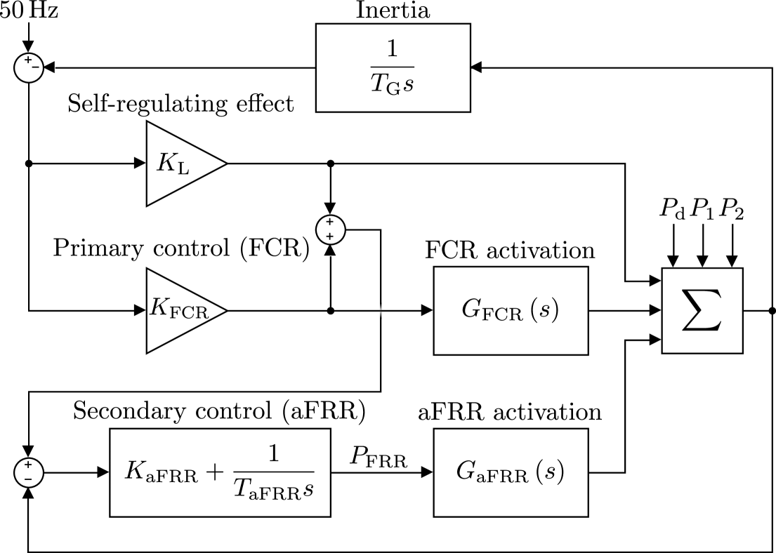
Figure 1: Single busbar model of a control area/control block.

In Fig. 2, different smart balancing reactions to a disturbance, caused by a power plant outage of 200MW at time $\displaystyle t=\qty{0}{min}$, are shown. The reactions vary in $\displaystyle T_{\mathrm{game}}$ and ramp rate $\displaystyle r$ ($\displaystyle|\mathrm{d}P/\mathrm{d}t|\leq r$) relative to the capacity $\displaystyle P_{b,\mathrm{max}}=\qty{150}{MW}$ of the asset that is used for smart balancing. Note that the scenario in which a BRP introduces schedule deviations by trading on the intraday market (also called financial smart balancing) is similar to $\displaystyle T_{\mathrm{game}}=\qty{1}{min}$. The effect of smart balancing by one ($\displaystyle\sum S_{b}=1$) or both ($\displaystyle\sum S_{b}=2$) of the BRPs on $\displaystyle P_{\mathrm{FRR}}$ is shown in Fig. 3 for games in which both BRPs use the same $\displaystyle T_{\mathrm{game}}$, $\displaystyle r$, and $\displaystyle P_{b,\mathrm{max}}$. The setup clearly matches the one given at the beginning of this section: when a single BRP reacts (dashed lines), they reduce the need for FRR, when both react (solid lines), it causes an overreaction. Multiple such overreactions can give rise to $\displaystyle P_{\mathrm{FRR}}$ oscillations.

Figure 2: Disturbance $\displaystyle P_{d}$ due to a power plant outage at time $\displaystyle t=\qty{0}{min}$ and smart balancing reaction $\displaystyle P_{b}$ for $\displaystyle T_{\mathrm{game}}=1,5,\qty{10}{min}$ with fast and slow assets and $\displaystyle P_{b,\mathrm{max}}=\qty{150}{MW}$.

Figure 3: Effect of smart balancing by one ($\displaystyle\sum S_{b}=1$) or both ($\displaystyle\sum S_{b}=2$) BRPs on the FRR power for symmetric scenarios, as defined in Fig. 2.

Based on Fig. 3, it is possible to calculate the gains or losses that each BRP encounters over the two shown ISPs for different strategy profiles. For calculating the payoffs, it is assumed that the marginal FRR prices scale linearly with $\displaystyle P_{\mathrm{FRR}}$. For the German imbalance pricing mechanism (2b and 3, abbreviated as DE-pricing), this means that the positive imbalance price is calculated as

$$C^{+}_{\mathrm{DE}}=\int_{\mathrm{ISP}}\max\left(P_{\mathrm{FRR}}(t),0\right)\,\mathrm{d}t\,.$$ (5)

The positive imbalance price for NL-pricing is given by

$$C^{+}_{\mathrm{NL}}=0.25\max_{t\in\mathrm{ISP}}P_{\mathrm{FRR}}(t)\,.$$ (6)

The factor 0.25(h) scales the maximum power to a period of 15min, so that the prices are in the same range for DE and NL. For the calculation of $\displaystyle C^{-}$, $\displaystyle\min$ is used instead of $\displaystyle\max$.

The payoff table for this smart balancing game is given in normal form in Table 1 using variables $\displaystyle g_{b}$ for the gain obtained when BRP $\displaystyle b$ choses action $\displaystyle S_{b}=1$, and $\displaystyle l_{b}$ for the loss suffered by BRP $\displaystyle b$ when both perform smart balancing. For symmetric games, like the ones matching Fig. 3, $\displaystyle g$ and $\displaystyle l$ can be used:

$$\displaystyle g_{1}=g_{2} \displaystyle=g>0\,,$$ (7a)

$$\displaystyle l_{1}=l_{2} \displaystyle=l>0\,.$$ (7b)

Values for $\displaystyle g$ and $\displaystyle l$, normalized to $\displaystyle\max(g)\!+\!\max(l)$, are given in Table 2 for different $\displaystyle T_{\mathrm{game}}$, $\displaystyle r$, and pricing mechanisms. For the same $\displaystyle T_{\mathrm{game}}$ and $\displaystyle r$, $\displaystyle g$ and $\displaystyle l$ are higher with NL-pricing. The ratio of $\displaystyle g$ to $\displaystyle g+l$ is systematically higher for DE-pricing.

Table 1: Payoff table for the smart balancing game.

		BRP $\displaystyle 2$
		$\displaystyle S_{2}=0$	$\displaystyle S_{2}=1$
BRP $\displaystyle 1$	$\displaystyle S_{1}=0$	$\displaystyle(0,0)$	$\displaystyle(0,g_{2})$
	$\displaystyle S_{1}=1$	$\displaystyle(g_{1},0)$	$\displaystyle(-l_{1},-l_{2})$

Table 2: Gains $\displaystyle g$ and losses $\displaystyle l$ for symmetric smart balancing games.

$\displaystyle T_{\mathrm{game}}$	$\displaystyle r$	DE-pricing			NL-pricing
$\displaystyle\left[\mathrm{min}\right]$	$\displaystyle\left[\mathrm{\%/min}\right]$	$\displaystyle g$	$\displaystyle l$	$\displaystyle\frac{g}{g+l}$	$\displaystyle g$	$\displaystyle l$	$\displaystyle\frac{g}{g+l}$
1	400	0.28	0.44	0.38	0.30	0.55	0.36
1	20	0.31	0.35	0.47	0.37	0.48	0.44
5	400	0.32	0.19	0.62	0.45	0.44	0.50
5	20	0.32	0.15	0.67	0.42	0.37	0.53
10	400	0.30	0.13	0.70	0.43	0.30	0.59
10	20	0.27	0.11	0.71	0.45	0.19	0.71

3 Analysis of the Smart Balancing Game

3.1 Nash Equilibrium Analysis

Table 2 holds the middle between the standard 2x2 games Battle of the Sexes and Game of Chicken (Faliszewski et al., 2024). As in those games, there are two pure strategy Nash equilibria (NEs): $\displaystyle(S_{1},S_{2})=(1,0)$ and $\displaystyle(S_{1},S_{2})=(0,1)$. These strategy profiles can be rewritten as $\displaystyle(p_{1}^{1},p_{2}^{1})=(1,0)$ and $\displaystyle(p_{1}^{1},p_{2}^{1})=(0,1)$ using the notation $\displaystyle p_{b}^{j}$ for the probability that BRP $\displaystyle b$ uses strategy $\displaystyle j$. With these strategy profiles, neither of the BRPs can improve their payoff through a one-sided change of strategy. The additional mixed-strategy NE can be written as

$$\displaystyle p_{b}^{1}=\frac{g}{g+l} \displaystyle\forall b\in\{1,2\}\,.$$ (8)

Also for this $\displaystyle p_{b}^{1}$, there is a no-regret equilibrium. Values for $\displaystyle g/(g+l)$ are listed in Table 2. The probability $\displaystyle p$ of an overreaction to the disturbance $\displaystyle P_{\mathrm{d}}$ is

$$p\left(\sum S_{b}=2\right)=p_{1}^{1}\,p_{2}^{1}\,.$$ (9)

For the pure strategy NEs, $\displaystyle p_{1}^{1}p_{2}^{1}=0$. For the mixed-strategy NE, $\displaystyle p_{1}^{1}p_{2}^{1}$ can be as high as 50% when $\displaystyle T_{\mathrm{min}}=\qty{10}{min}$ and $\displaystyle r=\qty{20}{\%/min}$. This means that 50% of the games played by BRPs using a mixed-strategy NE would result in overreactions for this scenario. Although this is a consequence of the optimal strategy of the BRPs, it is dangerous from a system stability perspective.

3.2 Equilibrium Selection

To analyse which NE would be selected when all players use rational criteria, the theory of equilibrium selection suggests the multilateral risk dominant NE, which is the NE with the smallest strategic risk, as the solution for games in which there is complete information, i.e., all players know the complete payoff table (Harsanyi, 1995). The risk dominant NE for the game in Table 1 is

$$\displaystyle(S_{1},S_{2})= \displaystyle(1,0), \frac{g_{1}}{g_{1}+l_{1}}>\frac{g_{2}}{g_{2}+l_{2}}$$ if , (10a)

$$\displaystyle(S_{1},S_{2})= \displaystyle(0,1), \frac{g_{1}}{g_{1}+l_{1}}<\frac{g_{2}}{g_{2}+l_{2}}$$ if . (10b)

For the symmetric games in Table 2, for which 7 holds, the conditions in 10b cannot be met and there is no single risk dominant NE. In such games, a correlated equilibrium, which requires previous communication between the players to alternate between the two pure strategy NE is proposed as rational solution (Harsanyi, 1995). If this is not possible, the mixed-strategy NE is a valid solution, but it is deemed undesirable, as it yields low payoffs and is nonpersistent (Harsanyi, 1995).

3.3 Experience-weighted Attraction Learning

Learning algorithms offer an alternative approach to study how equilibria arise in games. The experience-weighted attraction (EWA) model is often used, as it has been experimentally shown to describe the behaviour of real players relatively well, generalizes different learning rules, and only requires players to know their own payoffs (Camerer et al., 2002; Pangallo et al., 2022). In EWA, players play the same game repeatedly and discretely update two state variables to learn a strategy based on the payoffs $\displaystyle\pi_{b}$ they received (reinforcement learning) or could have received given the other player’s strategy (belief learning). The states are the experience $\displaystyle N[k]$, with $\displaystyle k$ the discrete time at which the states are updated, and the attraction $\displaystyle A_{b}^{j}[k]$ that player $\displaystyle b$ has towards strategy $\displaystyle j$. Using $\displaystyle-b$ for the opponent(s) of player $\displaystyle b$, and $\displaystyle I$ for the identity function, EWA is described by

$$\displaystyle N[k] \displaystyle=\left(1-\kappa\right)\left(1-\alpha\right)N[k-1]+1\,,$$ (11a)

$$\displaystyle A_{b}^{j}[k] \displaystyle=\frac{1}{N[k]}\Bigl{(}\left(1-\alpha\right)N[k-1]A_{b}^{j}[k-1]+\bigl{(}\delta+\left(1-\delta\right)I\left(j,S_{b}[k]\right)\bigr{)}\,\pi_{b}\left(j,S_{-b}[k]\right)\Bigr{)}\,,$$ (11b)

$$\displaystyle p_{b}^{j}[k] \displaystyle=\frac{\exp\left(\beta A_{b}^{j}[k]\right)}{\sum_{j^{\prime}}\exp\left(\beta A_{b}^{j^{\prime}}[k]\right)}\,,$$ (11c)

with parameters $\displaystyle\delta,\alpha,\kappa$ and $\displaystyle\beta$. $\displaystyle\delta$ ranges from 0 (reinforcement learning) to 1 (equal treatment of received payoffs and forgone payoffs). The memory loss $\displaystyle\alpha$ ranges from 0 (infinite memory) to 1 (no memory). The second depreciation parameter is $\displaystyle\kappa\in[0,1]$. Finally, $\displaystyle\beta\in(0,\infty]$ determines the intensity of choice. With $\displaystyle\beta=\infty$, $\displaystyle b$ always plays the strategy with the highest attraction. Mixed strategies are played for finite $\displaystyle\beta$, which is a reasonable assumption, both for human behaviour and strategies learned by machine learning algorithms.

A smart balancing game with $\displaystyle 10^{4}$ rounds is simulated to illustrate EWA in different scenarios, the parameters are chosen as $\displaystyle(\delta,\alpha,\kappa,\beta)=(0.25,0.05,1,1)$. These parameters indicate learning with a trade-off between reinforcement learning and belief learning, a small memory loss (valuing recent payoffs more) and mixed-strategies being played. The initial experience $\displaystyle N[0]$ is $\displaystyle 1$, and initial attractions $\displaystyle A_{b}^{j}[0]$ are sampled from the standard normal distribution, using the same initial attractions for different scenarios to enable comparisons. Instead of updating 11 after each game, 11 is updated repeatedly after playing $\displaystyle 100$ games with the same strategy, using the average payoffs obtained during those games in 11b. This type of batch learning is realistic for the smart balancing game, and corresponds with BRPs updating their strategy on a regular basis, but not after every single ISP.

This is implemented building further on Ferraz (2022). The results for a single learning realisation are shown in Fig. 4 for symmetric games with the DE-pricing with $\displaystyle T_{\mathrm{game}}=\qty{1}{min}$ and 10min, and both studied $\displaystyle r$. In the top figures, the probabilities $\displaystyle p_{b}^{1}$ that BRP $\displaystyle b$ performs smart balancing is shown, in the bottom figure the probability of overreactions 9 is shown. In Fig. 5, the results are given for NL-pricing.

Figure 4: Exemplary EWA learning dynamics with $\displaystyle(\delta,\alpha,\kappa,\beta)=(0.25,0.05,1,1)$ for DE-pricing: (top) probability for smart balancing by BRP $\displaystyle b$, (bottom) probability of overreactions caused by smart balancing.

Figure 5: Exemplary EWA learning dynamics with $\displaystyle(\delta,\alpha,\kappa,\beta)=(0.25,0.05,1,1)$ for NL-pricing: (top) probability for smart balancing by BRP $\displaystyle b$, (bottom) probability of overreactions caused by smart balancing.

The simulation converges to a pure stable fixed point (FP) in which one of the BRPs (in this case BRP 2) almost always performs smart balancing, and the other BRP has a low (non-zero) probability of performing smart balancing. The FP is pure because it lies in the vicinity of a pure NE (or at an alternative pure strategy profile) (Pangallo et al., 2022). The probability of overreactions occurring when these strategies are used can be higher during the learning phase than for the final strategy, as is seen, e.g., in Fig. 5 for $\displaystyle T_{\mathrm{game}}=\qty{1}{min}$, where the probability of an overreaction is higher than 10% for some $\displaystyle k<25$, but settles at less than 5% at $\displaystyle k=100$.

With different learning parameters, the smart balancing game converges to a unique pure stable FP or NE, multiple pure stable FPs or NEs, or a unique mixed stable FP (a FP that does not lie in the vicinity of a pure NE) (Galla and Farmer, 2013; Pangallo et al., 2022). Convergence to multiple FPs or NEs means that, depending on the initial attractions and experience, the dynamics converge to one of two stable solutions, as opposed to convergence to a unique stable solution. Because the payoffs of the BRPs are positively correlated (both BRPs are unhappy with the solutions $\displaystyle(S_{1},S_{2})=(1,1)$, and to a lesser extent with $\displaystyle(S_{1},S_{2})=(0,0)$ – they just don’t agree on which of the NEs is best), chaotic solutions or limit cycles cannot occur for $\displaystyle k\rightarrow\infty$ (Galla and Farmer, 2013). The convergence of the learning dynamics is good for the stability of the game, but convergence to FPs implies a non-zero probability of overreactions for $\displaystyle k\rightarrow\infty$. In such a case (e.g., Figs. 4 and 5), smart balancing sometimes causes overreactions when the game is played repeatedly, and BRPs cannot be expected to change their strategy because of this, as they are satisfied with the overall payoff of the smart balancing.

In order to study the asymptotic behaviour of EWA learning algorithms, a series of simulations is performed for a multidimensional sweep through the learning parameter space. It is assumed that the BRPs can play an infinite amount of games before updating 11, so that they are aware of the opponent’s mixed strategy. This is a common assumption that can be formulated analytically (Pangallo et al., 2022)). The limit $\displaystyle k\rightarrow\infty$ is approximated with $\displaystyle k=100$ in the simulations. The parameter ranges are $\displaystyle\delta\!\in\!\{0,0.25,0.5\}$, $\displaystyle\alpha\!\in\!\{0,0.05,0.1\}$, $\displaystyle\kappa\!\in\!\{0,0.5,1\}$, $\displaystyle\beta\!\in\!\{1,\infty\}$. For each combination of parameters, 100 simulations are made with different initial attractions sampled from the standard normal distribution. The parameter sweep is repeated for different pricing mechanisms, $\displaystyle T_{\mathrm{game}}$, and $\displaystyle r$.

The results for $\displaystyle T_{\mathrm{game}}=\qty{1}{min}$ and 10min, for DE- and NL-pricing are shown in Fig. 6. The scatter plot shows the probabilities of $\displaystyle p_{1}^{1}$ and $\displaystyle p_{2}^{1}$ for different parameter combinations. Additionally, the NEs are shown for the different scenarios (see Section 3.1). Finally, isolines for $\displaystyle p_{1}^{1}p_{2}^{1}$ show the probability of overreactions on baseline disturbance $\displaystyle P_{d}$ caused by smart balancing. The solutions shown in Figs. 4 and 5 are located near the upper left corner of the strategy spaces.

Figure 6: NEs and EWA convergence points for the smart balancing game for different parameter combinations in four scenarios, showing probability $\displaystyle p_{b}^{1}$ that BRP $\displaystyle b$ performs smart balancing. Isolines for $\displaystyle p_{1}^{1}p_{2}^{1}$ show the probability of overreactions in the power system introduced by smart balancing.

For all scenarios, simulations with convergence to pure and mixed FPs dominate the plot, and for certain parameter combinations, the steady-state solution results in overreactions for more than half of the ISPs when the game is played repeatedly ($\displaystyle p_{1}^{1}p_{2}^{1}>\qty{50}{\%}$). The parameters that lead to pure strategy solutions ($\displaystyle\beta=\infty$) cannot be distinguished, as they all lie in the corners of the strategy space. Games played at the beginning of the ISP (with small $\displaystyle T_{\mathrm{game}}$) have less probability of ending in an overreaction. Faster assets lower the probability of overreactions as well, though the overall impact of the ramp rate of the assets is small. The pricing mechanisms also influence the distribution of the FPs.

$\displaystyle T_{\mathrm{game}}$, $\displaystyle r$ and the pricing mechanism influence the outcome of the EWA learning because they affect $\displaystyle g$ and $\displaystyle l$. A systematic analysis of the impact of $\displaystyle g$ and $\displaystyle l$ on the distribution of the FPs and the probability of overreactions can be used to understand how the payoff table (Table 1) can be constructed to minimize the probability of overreactions to disturbances. An analytical solution of $\displaystyle p_{1}^{1}p_{2}^{1}$ in function of $\displaystyle g$, $\displaystyle l$ and the learning parameters does not exist, although progress is being made in creating a taxonomy of EWA in 2x2 games (Pangallo et al., 2022), where it is shown that both $\displaystyle l+g$ and $\displaystyle l-g$ play a role in the asymptotic behaviour of EWA.

In Table 3, the mean probability of overreactions and its standard deviation is given for the different symmetric scenarios studied throughout this paper, together with $\displaystyle l+g$ and $\displaystyle l-g$. For EWA learning with $\displaystyle\beta\!=\!\infty$, convergence to pure NEs generally occurs, except when cumulative attractions and infinite memory are used ($\displaystyle\kappa\!=\!1$, $\displaystyle\alpha\!=\!1$), in which case players can ‘lock’ into a certain strategy rapidly without exploring other possibilities (see Camerer et al. (2002), Pangallo et al. (2022, Fig. 2)). This results in a nonzero mean $\displaystyle p_{1}^{1}p_{2}^{1}$ and a significant standard deviation for the simulated parameter sweep. For $\displaystyle\beta=1$, it is seen that $\displaystyle p_{1}^{1}p_{2}^{1}$ decreases with increasing $\displaystyle l+g$ and $\displaystyle l-g$. In other words, when the absolute stakes are high (high $\displaystyle l+g$) and the potential losses are high compared with the potential gains (high $\displaystyle l-g$), the probability of both BRPs performing smart balancing at the same time, causing an overreaction, lowers. That both $\displaystyle l+g$ and $\displaystyle l-g$ affect $\displaystyle p_{1}^{1}p_{2}^{1}$ is clear from the results with NL-pricing for $\displaystyle T_{\mathrm{game}}=\qty{5}{min}$, $\displaystyle r=\qty{400}{\%}$ and $\displaystyle T_{\mathrm{game}}=\qty{10}{min}$, $\displaystyle r=\qty{20}{\%}$. These scenarios have the highest normalized value for $\displaystyle l+g$ ($\displaystyle 0.89$) and the lowest value for $\displaystyle l-g$ ($\displaystyle-0.26$), respectively. However, the scenario with $\displaystyle T_{\mathrm{game}}=\qty{5}{min}$ and $\displaystyle r=\qty{400}{\%}$ performs bad on $\displaystyle l-g$, and the second scenario performs good on $\displaystyle l+g$, so that they do not end up with the lowest, respectively highest, probability of overreactions.

Table 3: Mean overreaction probability $\displaystyle p_{1}^{1}p_{2}^{1}$ for a multidimensional parameter sweep of EWA dynamics, also showing $\displaystyle l\pm g$.

	$\displaystyle T_{\mathrm{game}}$	$\displaystyle r$	$\displaystyle l+g$	$\displaystyle\;l-g$	$\displaystyle\text{mean}\,p_{1}^{1}p_{2}^{1}$ ($\displaystyle\text{std}\,p_{1}^{1}p_{2}^{1}$)
	$\displaystyle\left[\mathrm{min}\right]$	$\displaystyle\left[\mathrm{\%/min}\right]$			$\displaystyle\beta=1$	$\displaystyle\beta=\infty$
DE-pricing	1	400	0.72	$\displaystyle\phantom{-}0.17$	15.6 (9.1)	0.1 (3.6)
	1	20	0.66	$\displaystyle\phantom{-}0.04$	17.5 (9.5)	0.2 (4.3)
	5	400	0.51	$\displaystyle-0.13$	22.1 (10.2)	0.3 (5.1)
	5	20	0.47	$\displaystyle-0.16$	23.9 (10.3)	0.5 (7.3)
	10	400	0.42	$\displaystyle-0.17$	24.9 (10.2)	0.2 (4.3)
	10	20	0.39	$\displaystyle-0.16$	25.5 (9.9)	0.1 (3.3)
NL-pricing	1	400	0.85	$\displaystyle\phantom{-}0.24$	14.3 (9.2)	0.1 (3.3)
	1	20	0.86	$\displaystyle\phantom{-}0.11$	15.4 (9.7)	0.2 (4.7)
	5	400	0.89	$\displaystyle-0.01$	16.4 (10.3)	0.2 (4.5)
	5	20	0.79	$\displaystyle-0.05$	17.6 (10.3)	0.4 (5.9)
	10	400	0.73	$\displaystyle-0.13$	19.2 (10.5)	0.3 (5.4)
	10	20	0.64	$\displaystyle-0.26$	23.1 (11.2)	0.1 (3.8)

4 Conclusions and Final Remarks

Although smart balancing is meant to reduce the control area imbalance, it is possible that the combined smart balancing of multiple BRPs overcompensates the baseline disturbance $\displaystyle P_{d}$, causing an overreaction. This is studied in a 2x2 game (Table 1) based on dynamic power system simulations, in which two BRPs can choose whether to perform smart balancing, receiving gain $\displaystyle g$ if they are the only one to perform smart balancing, and loss $\displaystyle l$ if they both perform smart balancing. It is assumed that the BRPs know $\displaystyle g$ and $\displaystyle l$ at the time at which the game is played. Different scenarios are used to analyse the effects of the different pricing mechanisms, as well as variations in the time at which the game takes place and the ramp rate of the used assets.

In this framework, the risk of smart balancing leading to overreactions to disturbances in the power system is shown to be inherent to the topology of the game: Neither equilibrium selection theory, nor EWA learning, results in steady-state solutions without stochastic overreactions in repeated play. Depending on $\displaystyle g$, $\displaystyle l$, and the learning dynamics, the probability of overreactions is up to 50% for steady-state fixed points. Learning dynamics can cause a temporary increase in this probability. This can happen when a change in $\displaystyle g$ or $\displaystyle l$ triggers new learning dynamics, e.g., when changes are made to the imbalance pricing mechanism or the NRT data publication, or if new players enter the smart balancing game.

It is found that the probability of overreactions to disturbances can be reduced by increasing the stakes of the game (high $\displaystyle l+g$) and having a high potential loss relative to the potential gains (high $\displaystyle l-g$). The nonlinear effects in the imbalance pricing (the use of binary criteria, marginal prices and the multiplication of smart balancing energy with price) make it difficult to define general conditions that lead to the lowest risk of overreactions. For the considered scenarios with a power plant outage at the beginning of the ISP, it is beneficial when BRPs play the game early in the ISP and use fast assets. In these scenarios, the pricing mechanism used in the Netherlands leads to lower probability of overreactions than the German pricing mechanism.

Some of the measures taken by the Dutch TSO to reduce the negative effects of smart balancing are counterproductive from a game theoretical perspective. The increase in delay for the publication of NRT data, “done to increase the uncertainty of a result of a response based on the balance delta information” (TenneT, 2024a), could result in games being played later in the ISP, increasing the probability of overreactions. Clarity about potential payoffs (both $\displaystyle g$ and $\displaystyle l$) as early as possible in the ISP would be beneficial. An additional positive measure would be a communication channel between BRPs, which would make correlated equilibrium solutions possible (Section 3.2), maximizing payoffs for the BRPs and minimizing the stability risk. Further research could investigate whether this can be accomplished through the publication of additional NRT data.

Because only the probability of overreactions is studied, the size and dynamics of the overreaction are not part of this study. In Fig. 3, it is seen that a ramp rate limit of $\displaystyle r=\qty{20}{\%/min}$ on smart balancing assets slows down the dynamics of $\displaystyle P_{\mathrm{FRR}}$, achieving a positive effect on the system stability, even when this measure has a (limited) negative effect on the probability of overreactions. Most findings of this study are expected to hold for an $\displaystyle n$ player game with multiple decision possibilities and asymmetric games, although for asymmetric games, equilibrium selection often results in pure NEs (see 10b). For $\displaystyle n$ player games, the probability of $\displaystyle\left|E_{\mathrm{FRR}}\right|$ being larger with than without smart balancing can be investigated. The effect of multiple consecutive decisions in sequential games (e.g., when BRPs notice an overreaction) can also be studied in future research.

References

- ENTSO-E [2018] ENTSO-E. Electricity Balancing in Europe, November 2018. URL https://eepublicdownloads.entsoe.eu/clean-documents/Network%20codes%20documents/NC%20EB/entso-e_balancing_in%20_europe_report_Nov2018_web.pdf.
- [2] Netcode elektriciteit. URL https://wetten.overheid.nl/BWBR0037940/2025-01-01#Hoofdstuk10.
- Elia Transmission Belgium [2019] Elia Transmission Belgium. End User Documentation “1-minute publications”, August 2019. URL www.elia.be/-/media/project/elia/elia-site/grid-data/balancing/20190827_end-user-documentation-elia1-minute-publications.pdf.
- TenneT [2024a] TenneT. Summary balance delta publication (Follow-up of the webinar on November 2, 2024), November 2024a. URL https://tennet-drupal.s3.eu-central-1.amazonaws.com/default/2024-11/Summary%20balance%20delta%20publication%20webinar.pdf.
- Röben [2022] Felix Röben. Smart Balancing of Electrical Power Transparent Real-Time Market for Cost-Efficient Power Balancing. PhD thesis, Europa Universität Flensburg, 2022. URL https://d-nb.info/127953821X/34.
- TenneT [2024b] TenneT. Power imbalance oscillations: Balance delta delay and additional measures (TenneT Market News), November 2024b. URL https://www.tennet.eu/grids-and-markets/market-news.
- Maucher et al. [2022] Philipp Maucher, Simon Remppis, Dominik Schlipf, and Hendrik Lens. Control Aspects of the Interzonal Exchange of automatic Frequency Restoration Reserves. IFAC-PapersOnLine, 55(9):30–35, 2022. ISSN 2405-8963.
- Faliszewski et al. [2024] Piotr Faliszewski, Irene Rothe, and Jörg Rothe. Noncooperative Game Theory, pages 43–137. Springer Nature Switzerland, 2024. ISBN 978-3-031-60099-9. doi: 10.1007/978-3-031-60099-9˙2.
- Harsanyi [1995] John C. Harsanyi. A new theory of equilibrium selection for games with complete information. Games and Economic Behavior, 8(1):91–122, 1995. ISSN 08998256. doi: 10.1016/S0899-8256(05)80018-1.
- Camerer et al. [2002] Colin F. Camerer, David Hsia, and Teck-Hua Ho. EWA Learning in Bilateral Call Markets. In Rami Zwick and Amnon Rapoport, editors, Experimental Business Research, pages 255–284. Springer US, Boston, MA, 2002. ISBN 978-1-4757-5196-3. doi: 10.1007/978-1-4757-5196-3˙11.
- Pangallo et al. [2022] Marco Pangallo, James B.T. Sanders, Tobias Galla, and J. Doyne Farmer. Towards a taxonomy of learning dynamics in 2 × 2 games. Games and Economic Behavior, 132:1–21, 2022. ISSN 08998256. doi: 10.1016/j.geb.2021.11.015.
- Ferraz [2022] Vinicius Ferraz. Dynamic Equilibria Prediction: Experience-Weighted Attraction (EWA), 2022. URL https://doi.org/10.25937/q2xt-rj46. Publisher: CoMSES.Net.
- Galla and Farmer [2013] Tobias Galla and J. Doyne Farmer. Complex dynamics in learning complicated games. Proceedings of the National Academy of Sciences, 110(4):1232–1236, 2013. doi: 10.1073/pnas.1109672110.