Precise Static Identification of Ethereum Storage Variables

Abstract.

Smart contracts are small programs that run autonomously on the blockchain, using it as their persistent memory. The predominant platform for smart contracts is the Ethereum VM (EVM). In EVM smart contracts, a problem with significant applications is to identify data structures (in blockchain state, a.k.a. “storage”), given only the deployed smart contract code. The problem has been highly challenging and has often been considered nearly impossible to address satisfactorily. (For reference, the latest state-of-the-art research tool fails to recover nearly all complex data structures and scales to under 50% of contracts.) Much of the complication is that the main on-chain data structures (mappings and arrays) have their locations derived dynamically through code execution.

We propose sophisticated static analysis techniques to solve the identification of on-chain data structures with extremely high fidelity and completeness. Our analysis scales nearly universally and recovers deep data structures. Our techniques are able to identify the exact types of data structures with 98.6% precision and at least 92.6% recall, compared to a state-of-the-art tool managing 80.8% and 68.2% respectively. Strikingly, the analysis is often more complete than the storage description that the compiler itself produces, with full access to the source code.

1. Introduction

Smart contracts on programmable blockchains have been successfully used to implement complex applications, mostly of a financial nature (Werner et al., 2023). The dominant platform for smart contracts is the Ethereum VM (EVM): the execution layer behind blockchains such as Ethereum, Arbitrum, Optimism, Binance, Base, and many more. Millions of smart contracts have been deployed on these chains and can be invoked on-demand. Many thousands of them are in active use every day.

To enable the persistence of data between different blockchain transactions, contracts employ the blockchain as their persistent memory, to save their state. In EVM terms, this persistent memory is called “storage” and is accessed using special random-access instructions. A challenge of high value has emerged out of the use of storage in smart contracts: recovering high-level storage structures from the deployed form of the smart contract, i.e., from EVM bytecode. This task is crucial for several applications:

• Security Analysis: A number of smart contract vulnerabilities arise from incorrect handling of storage variables, such as storage collisions in upgradable contracts (Ruaro et al., 2024). Precise modeling of storage is required for detecting such vulnerabilities.

• Decompilation and Reverse Engineering: Tools (Grech et al., 2022; Kolinko and Palkeo, 2020; Becker, 2023) that decompile EVM bytecode back to high-level code rely on storage modeling to reconstruct variable declarations and data structures (Li et al., 2024).

• Off-chain Applications: Blockchain explorers, debuggers, and other off-chain tools need to interpret storage data to provide meaningful information to users. They often rely on compiler-generated metadata, which may be incomplete or unavailable (etherscan.io, 2017) for interesting smart contracts like proprietary bots or hacker contracts.

• Static Analysis and Verification: Precise storage modeling enables advanced static analysis and formal verification of smart contracts, facilitating the detection of bugs and the proof of correctness (Grech et al., 2018; Brent et al., 2020; Yang et al., 2024; Chen et al., 2024b).

Smart contracts are written overwhelmingly in the Solidity language, which allows developers to define storage variables ranging from simple value types to complex, arbitrarily nested data structures such as arrays, mappings, and structs.

However, when Solidity code is compiled into EVM bytecode, much of the high-level structure and type information is lost. This is because the EVM’s permanent storage is a simple key-value store mapping 256-bit keys to 256-bit values. Due to the luxury of having a large key space, the default pattern for high-level languages targeting the EVM is to translate high-level constructs into low-level storage access patterns using cryptographic hashing and arithmetic operations to compute storage slots dynamically. This transformation creates a significant gap between the high-level representation of storage variables and the low-level state of permanent storage reflected on the blockchain.

Existing approaches to storage modeling face significant limitations. Early frameworks (Albert et al., 2018; Tsankov et al., 2018) often reasoned about storage operations only when storage indexes were constants, sacrificing precision or completeness when dealing with dynamic data structures. While some tools (Grech et al., 2018; Brent et al., 2020) introduced methods to infer high-level storage structures, they lacked support for arbitrarily nested data structures and complex storage patterns. Recent tools like VarLifter (Li et al., 2024) attempt to recover storage layouts but struggle with scalability and completeness, failing to produce output for a substantial portion of real-world contracts.

Contributions. This paper introduces dyels, a static analysis approach that accurately infers high-level storage structures from EVM bytecode. Our key contributions are:

• Static Storage Modeling: We develop a novel static analysis that fully supports arbitrarily nested composite data structures in Solidity. By employing a recursive storage analysis, dyels scalably and precisely reconstructs complex storage layouts from low-level bytecode.

• Evaluation Against Existing Tools: We find the current state-of-the-art tool, VarLifter (Li et al., 2024), to terminate on only 41.2% of contracts. When successful, VarLifter misses over 30% of storage variables, including most non-trivial structures. This performance underscores the difficulty of the problem being solved. In comparison, dyels analyzes 99.5% of contracts and provides higher-fidelity results, recovering the vast majority (92%) of storage structures with excellent precision (98%).

• Enhanced Completeness Beyond Compiler Metadata: We show that dyels can infer storage variables and structures not present in compiler-generated metadata, particularly those involving low-level storage patterns common in upgradable contracts. This enhancement provides a more complete understanding of the contract’s storage layout.

The core of dyels is released as open-source software as part of the Gigahorse lifting toolchain   and has seen significant adoption in both industry and academia. Its output is integrated into the decompilation of https://app.dedaub.com, the Dedaub security and decompilation tool suite used by over 6,000 registered users.

2. Background

We next provide background on the Ethereum Virtual Machine and its storage model.

2.1. Ethereum and the Ethereum Virtual Machine

Ethereum is a decentralized blockchain platform that enables the execution of smart contracts—autonomous programs that run on the blockchain. Smart contracts are predominantly written in the Solidity high-level language and are compiled into bytecode for execution on the Ethereum Virtual Machine (EVM). The EVM has dominated as an execution platform and has been adopted by most other programmable blockchains.

The EVM is a stack-based virtual machine designed to execute smart contracts securely and deterministically. It operates on 256-bit words, utilizes its own stack, memory, transient storage and persistent storage, and provides a Turing-complete execution environment. This paper focuses on persistent storage or just storage.

2.2. EVM Bytecode Format and Execution Model

EVM bytecode is a sequence of instructions, each represented by a single-byte opcode (with an immediate argument for PUSH opcodes). The EVM supports a rich, albeit unconventional set of operations, which includes anything from arithmetic, logic, control flow, hashing, and state and memory interaction.

As a stack-based machine, most EVM opcodes perform computations using a stack of 256-bit words, when such an opcode has a fixed operand or return size. The EVM also features different kinds of state. Memory is a dense addressable byte array that is cleared at the end of each transaction with a smart contract (from the outside or nested, via calls from one contract to the next). A recent addition is transient storage, which is cleared at the end of the outermost transaction.

2.3. Storage in the EVM

At the EVM level, persistent storage (or simply storage) is a persistent key-value store where both keys and values are 256-bit words. Storage maintains the state of a contract between transactions. Storage is simply a sparse word array indexed by 256-bit words, spanning from keys $0$ to $2^{256}-1$.

High-level languages like Solidity provide structured data types such as integers, arrays, mappings, and structs. The Solidity compiler maps these high-level constructs to EVM storage using specific patterns, now also widely-adopted in other compilers.

The EVM only allows reading from and writing to storage using the SLOAD and SSTORE instructions, both of which index storage using a 32-byte index value, with the value read or written also being fixed at 32 bytes. As high-level languages need to implement arbitrarily complex data structures using such very low-level primitives, there is a huge disparity between the source and bytecode representations.

2.4. EVM Storage Model and Solidity Storage Layout

During compilation, the Solidity compiler generally predictably orders smart contract storage variables using a deterministic heuristic (e.g., by employing C3 linearization upon inheritance) and assigns a slot $p$ to each variable, and accumulates $p$ by an appropriate amount at each step.

The following cases briefly capture the mapping of high-level constructs to EVM storage:

• Value Types: Simple value types (e.g., uint256, bool, address) are stored in sequential storage slots starting from slot $0$. To optimize space, multiple small values may be packed into a single 32-byte storage slot. For example, two uint128 variables can share one slot, and smaller types like bool and uint8 can be packed together.

• Static Arrays: Fixed-size arrays are stored by sequentially allocating storage slots for each element. For an array declared as T[n], where T is the element type and n is the fixed size, elements are stored starting from slot $p$, the assigned slot of the array variable. The element at index $i$ is stored at slot $p+i$.

• Dynamic Arrays: Dynamic arrays store their length at a fixed slot $p$, and their elements are stored starting from the Keccak-256 hash of slot $p$. (This is a cryptographic hash function, expected to be collision-free.) Specifically, element $i$ is stored at position $\mathit{keccak256}(p)+i$ where $p$ is the slot assigned to the array variable. This allows for arrays of arbitrary length without preallocating storage slots.

• Mappings: Mappings use a hashing scheme to avoid key collisions. A mapping declared as mapping(K => V) at slot $p$ stores a value associated with key $k$ at $\mathit{keccak256}\left(\mathit{encode}(k)\parallel p\right)$ where $\parallel$ denotes concatenation, and $\mathit{encode}(k)$ is the padded representation of key $k$. This ensures that each key-value pair in the mapping has a unique storage slot.

• Structs: Structs are stored by sequentially allocating storage slots for each of their members, similar to value types. For a struct declared as struct S { ... } and a variable of type S assigned to slot $p$, its members are stored starting from slot $p$. If a struct contains members that are arrays or mappings, the storage rules for arrays and mappings are applied recursively to those members.

The recursive nature of these storage rules makes static modeling of storage complex, especially when only the EVM bytecode is available. For instance, mappings and dynamic arrays involve runtime computations of storage slots using hash functions, which are challenging to resolve statically. Additionally, the packing of multiple variables into a single storage slot requires bit-level instruction analysis to accurately extract individual variables.

3. Smart Contract Storage Patterns

We next show a simple smart contract that will serve as an example to explain how the most common data structures provided by Solidity are implemented in the low-level EVM bytecode.

⬇

1 contract StorageExample {

2 uint256 public supply; // slot 0x0

3 address public owner; // slot 0x1

4 bool public isPaused; // slot 0x1

5 uint256[] public supplies; // slot 0x2

6 mapping (address => bool) public admins; // slot 0x3

7 struct vals {uint256 field0; uint256 field1;}

8 mapping (address => mapping(uint256 => vals)) public complex; // slot 0x4

9 }

Figure 1. Example Smart Contract

3.1. Low-Level Implementation Patterns

For our example contract in Figure 1, the storage layout translates to the following low-level operations, also shown schematically in Figure 2:

• Simple Values (slot 0x0): The supply variable occupies a full slot:

  • Load: SLOAD(0x0)

  • Store: SSTORE(0x0) = newSupply

• Packed Values (slot 0x1): The owner (20 bytes) and isPaused (1 byte) share slot 0x1:

  • Load owner: SLOAD(0x1) followed by
    AND(loaded, 0xffffffffffffffffffffffffffffffffffffffff)

  • Load isPaused: SLOAD(0x1) followed by AND(SHR(0xa0, loaded), 0xff).
    The masked variable is often followed by two ISZERO(ISZERO(masked)).

  • Store requires reading existing value, masking, and combining with new value.

• Dynamic Array (slot 0x2): For supplies:

  • Length access: length = SLOAD(0x2)

  • Element $i$ access: SLOAD($\mathtt{keccak256}({\small\texttt{0x2}})+i$)

  • Store: SSTORE($\mathtt{keccak256}({\small\texttt{0x2}})+i$) = value

• Mapping (slot 0x3): For admins:

  • Key $k$ access: SLOAD($\mathtt{keccak256}(\mathtt{pad32}(k)\parallel{\small\texttt{0x3}})$)

  • Store: SSTORE($\mathtt{keccak256}(\mathtt{pad32}(k)\parallel{\small\texttt{0x3}})$) = value

• Nested Mapping (slot 0x4): For complex:

  • For keys $k_{1}$, $k_{2}$:
    field0 is accessed using: SLOAD($\mathtt{keccak256}(\mathtt{pad32}(k_{2})\parallel\mathtt{keccak256}(\mathtt{pad32}(k_{1})\parallel{\small\texttt{0x4}}))$)
    field1 is accessed using: SLOAD($\mathtt{keccak256}(\mathtt{pad32}(k_{2})\parallel\mathtt{keccak256}(\mathtt{pad32}(k_{1})\parallel{\small\texttt{0x4}}))+1$)

Figure 2. Low-level Storage Layout Implementation of our example in Figure 1

3.2. Low-level Storage Patterns in High-level Code

Although high-level storage patterns allow developers to implement powerful protocols, making use of complex high-level data structures, the storage allocation algorithm has its drawbacks. Solidity does not offer a high-level way to override the assigned storage slot of a variable declaring it at an arbitrary slot. This functionality is needed by various standards requiring compatible storage layouts. The most important such standard is ERC-1967 (Palladino et al., 2019), standardizing the allocated storage slots to be used for the implementation, admin, and beacon contract addresses of upgradable proxy contracts. To support these standard patterns developers make use of Solidity’s inline assembly (Chaliasos et al., 2022), as shown in Figure 3.

⬇

1 bytes32 internal constant _ADMIN_SLOT =

2 0xb53127684a568b3173ae13b9f8a6016e243e63b6e8ee1178d6a717850b5d6103;

3

4 function _getAdmin() internal view returns (address) {

5 return StorageSlot.getAddressSlot(_ADMIN_SLOT).value;

6 } // returns the value of the address typed variable stored at _ADMIN_SLOT

7

8 struct AddressSlot {

9 address value;

10 }

11

12 // Returns an ‘AddressSlot‘ with member ‘value‘ located at ‘slot‘.

13 function getAddressSlot(bytes32 slot) internal pure returns (AddressSlot storage r) {

14 assembly {

15 r.slot := slot

16 }

17 }

Figure 3. Low-level code implementing the ERC-1967 standard.

Such low-level code patterns allow users to use storage variables that are not declared as such. Thus, these variables are unknown to the Solidity compiler, and are not included in its storage layout metadata. This incompleteness of the compiler-produced metadata will be examined in our evaluation of Section 7.

4. Analysis Preliminaries

The dyels approach is a static analysis of the program’s (smart contract’s) code that identifies the low-level patterns that the Solidity compiler produces to implement the high-level features presented in Section 3. The challenge is to maintain the right level of analysis precision and scalability/computability, since the analysis needs to model the derivation structure of arbitrary dynamic numerical quantities.

4.1. Input

$V$: set of variables	$S$: set of program statements
$C$: set of 256-bit numbers	Int: set of 16-bit numbers

Figure 4. Type domain definitions

$\mathit{I}$ : $\mathsf{r}$ := $\mathsf{LOAD}$($\mathsf{iv}$) $|$ $\mathsf{r}$ $\in$ $V$, $\mathit{I}$ $\in$ $S$, $\mathsf{iv}$ $\in$ $V$

SLOAD statement $\mathit{I}$ loads into $\mathsf{r}$ the value of storage location pointed-to by $\mathsf{iv}$

$\mathit{I}$ : $\mathsf{STORE}$($\mathsf{iv}$) := $\mathsf{u}$ $|$ $\mathit{I}$ $\in$ $S$, $\mathsf{iv}$ $\in$ $V$, $\mathsf{u}$ $\in$ $V$

SSTORE statement $\mathit{I}$ stores the value of $\mathsf{u}$ into the storage location pointed to by $\mathsf{iv}$

$\mathsf{r}$ := $\mathsf{ADD/SUB/MUL}$($\mathsf{a,b}$) $|$ $\mathsf{r}$ $\in$ $V$, $\mathsf{a}$ $\in$ $V\cup C$, $\mathsf{b}$ $\in$ $V\cup C$

Binary arithmetic operation over variable or constant operands $\mathsf{a,b}$

v $\to$ c $|$ $\mathsf{v}$ $\in$ $V$, $\mathsf{c}$ $\in$ $C$

Constant folding and constant propagation analysis. $\mathsf{v}$ has constant value $\mathsf{c}$.

f $\rightsquigarrow$ t $|$ $\mathsf{f}$ $\in$ $V$, $\mathsf{t}$ $\in$ $V$

Limited data flows analysis: $\mathsf{f}$ flows to $\mathsf{t}$ through low-level shifting and masking operations.

$\mathsf{l}$ := $\phi$($\mathsf{u}$) $|$ $\mathsf{l}$ $\in$ $V$, $\mathsf{u}$ $\in$ $V$

SSA PHI instructions

$\mathsf{r}$ := $\mathsf{LowBytesMask}$($\mathsf{u,w}$) $|$ $\mathsf{r}$ $\in$ $V$, $\mathsf{u}$ $\in$ $V$, $\mathsf{w}$ $\in$ Int

Masking operation ($\mathsf{w}$ bytes of mask width) used in casting $\mathsf{u}$ to value types

uintX, intX, address, bool

$\mathsf{r}$ := $\mathsf{HighBytesMask}$($\mathsf{u,w}$) $|$ $\mathsf{r}$ $\in$ $V$, $\mathsf{u}$ $\in$ $V$, $\mathsf{w}$ $\in$ Int

Masking operation ($\mathsf{w}$ bytes of mask width) used in casting $\mathsf{u}$ to the bytes$X$ value types

$\mathsf{r}$ := $\mathsf{LShift/RShift}$($\mathsf{u,n}$) $|$ $\mathsf{r}$ $\in$ $V$, $\mathsf{u}$ $\in$ $V$, $\mathsf{n}$ $\in$ Int

Variable $\mathsf{u}$ is shifted to the left/right by $\mathsf{n}$ bytes.

$\mathsf{r}$ := $\mathsf{BooleanCast}$($\mathsf{u}$) $|$ $\mathsf{r}$ $\in$ $V$, $\mathsf{u}$ $\in$ $V$

Low-level cast to boolean using two consecutive ISZERO operations.

$\mathsf{HighLevelOpUse}$($\mathsf{v}$) $|$ $\mathsf{v}$ $\in$ $V$

Variable $\mathsf{v}$ is used in high-level operation (e.g., non-storage-address computation, calls).

$\mathsf{r}$ := $\mathsf{HASH}$($\mathsf{\mathsf{a},*}$) $|$ $\mathsf{r}$ $\in$ $V$, $\mathsf{a}$ $\in$ $V$

SHA3 operation that computes the keccak256 hash of a variable number of args, storing it into $\mathsf{r}$

Figure 5. Input relation definitions

Figures 4 and 5 define the input schema for our analysis. (In using these predicates, we drop elements that are not needed for the rule at hand, e.g., we may write “$\mathsf{r}$ := $\mathsf{LOAD}$($\mathsf{iv}$)” instead of “I : $\mathsf{r}$ := $\mathsf{LOAD}$($\mathsf{iv}$)” when the instruction identifier I is unused.)

While these types and relations originate from the Elipmoc/Gigahorse lifter toolchain (Grech et al., 2019, 2022; Lagouvardos et al., 2020), our approach is not restricted to this framework. Instead, it can be applied to any mature decompilation framework that lifts the stack-based EVM bytecode into a register-based static-single-assignment (SSA) representation.

Some relations in Figure 5 directly correspond to the register-based representation, such as LOAD and STORE, while others, like ADD, SUB, and MUL, also incorporate the results of a constant folding and constant propagation analysis. Predicates handling masking and shifting are convenience wrappers for low-level arithmetic and bitwise operations of variables and constants: LowBytesMask and HighBytesMask correspond to operation patterns that use AND instructions; LShift to patterns with MUL and SHL (a left-shift); RShift to patterns with DIV and SHR (right-shift).

Finally, the HASH relation, which supports the low-level implementation patterns presented in Section 3, stems from the EVM “memory” analysis (Lagouvardos et al., 2020) built on top of Gigahorse. While this specific implementation is tied to Gigahorse, similar EVM memory analyses (Grossman et al., 2024; Albert et al., 2023) have been developed on top of other SSA-based analysis frameworks.

4.2. Analysis (Un)soundness and (In)completeness

The dyels analysis is sound and complete for common, disciplined data structure manipulation and compilation patterns, modulo errors of the underlying decompiler.

However, in practice no technique can be either sound or complete under realistic assumptions: the program can have arbitrarily complex (Turing-complete) logic for accessing storage, leading to either false positives or false negatives. For instance, a storage slot can be accessed via arbitrary arithmetic to compute its address; the knowledge that a field is 64-bit long (inside a 256-bit word) could be reflected not in a straightforward AND/OR bitwise mask but implicitly using mathematical properties reflected in a multiplication; a storage address can be computed via a different hash function, implemented explicitly in code; etc. There is no guarantee as to what the cleverness of the compiler or of the human programmer can obscure. (Notably, the human programmer only needs to use minimal inline assembly, e.g., a single statement, as in Figure 3, and can otherwise compute storage addresses using any high-level algorithmic logic.)

Therefore, the evaluation of dyels’s effectiveness involves “precision” and “recall” metrics. These capture experimentally the degree of (un)soundness, i.e., inferences that are wrong, and the degree of (in)completeness, i.e., ground truth that is missed, respectively.

5. Structure Identification

The dyels analysis has two main parts: a) discovering the structure of a program’s storage layout (e.g., which structures are nested arrays or mappings); b) discovering the types of data stored in every entry of each structure. This section presents the first part: how to identify the data structures in a smart contract’s storage.

5.1. Storage Index Value-flow Analysis

The backbone of the analysis is a value-flow analysis that computes the values of all potential storage index expressions, and then uses the ones that end up being used in actual storage operations to identify the constructs in the program’s storage layout.

lcll type $\mathit{SInd}$ =$\mathit{Const}_{\mathit{I}}$(c: $C$)
$|$ $\mathit{ArrA}_{\mathit{I}}$(par: $\mathit{SInd}$, iv: $V$)
$|$ $\mathit{ArrD}_{\mathit{I}}$(par: $\mathit{SInd}$)
$|$ $\mathit{Map}_{\mathit{I}}$(par: $\mathit{SInd}$, kv: $V$)
$|$ $\mathit{Offs}_{\mathit{I}}$(par: $\mathit{SInd}$, of: Int)

Figure 6. Vocabulary of storage index value expressions

Figure 6 presents our definition of the storage index values for our value-flow analysis. The Algebraic Data Type (ADT) in the figure aims to capture accesses to Solidity’s arbitrarily-nested high-level structures. The ADT effectively defines what the analysis can infer about potential storage indexes.

$\mathit{Const}_{\mathit{I}}$ is the only non-recursive kind of $\mathit{SInd}$ type. Every storage index will include a $\mathit{Const}_{\mathit{I}}$ as the leaf of its ADT value, since all high-level storage structures are assigned a constant offset by the compiler. The rest of the storage index types are recursively built on top of a pre-existing $\mathit{SInd}$ instantiation, encoded as par (“par” for “parent”). These include $\mathit{ArrA}_{\mathit{I}}$ and $\mathit{ArrD}_{\mathit{I}}$ used to model operations on dynamic arrays, $\mathit{Map}_{\mathit{I}}$ for mapping operations, and $\mathit{Offs}_{\mathit{I}}$, which enables supporting struct accesses. In addition to the par index, $\mathit{SInd}$ values that model an index to a high-level data structure (array or mapping) also include the index or key variables.

To compute the possible storage indexes for arbitrarily-nested data structures we define our analysis as a set of recursive inference rules. The rules are faithfully transcribed from a fully mechanized implementation, so they should be precise, modulo mathematical shorthands used for conciseness.

The analysis first computes two new relations.

$\mathsf{v}$ $\stackrel{{\scriptstyle S}}{{\to}}$ $\mathsf{si}$ $\big{|}$ $\mathsf{v}$ $\in$ V, $\mathsf{si}$ $\in$ $\mathit{SInd}$

Storage Index Overapproximation: Variable $\mathsf{v}$ holds potential storage index $\mathsf{si}$.

$\Downarrow$ $\mathsf{si}$ $|$ $\mathsf{si}$ $\in$ $\mathit{SInd}$

Actual Storage Index: $\mathsf{si}$ ends up being used in a storage loading/storing operation.

5.1.1. Storage Index Overapproximation

Figure 7 contains our analysis logic for overapproximating the possible storage index values.

$$\textsc{(Base)}\quad\inferrule{\mathsf{v}\to\mathsf{c}}{\mathsf{v}\stackrel{{\scriptstyle S}}{{\to}}\mathit{Const}_{\mathit{I}}(\mathsf{c})}$$

$$\textsc{(Mapping)}\quad\inferrule{\mathsf{pv}\stackrel{{\scriptstyle S}}{{\to}}\mathsf{si}\\ \mathsf{v}:=\mathsf{HASH}(\mathsf{kv},\mathsf{pv})}{\mathsf{v}\stackrel{{\scriptstyle S}}{{\to}}\mathit{Map}_{\mathit{I}}(\mathsf{si},\mathsf{kv})}$$

$$\textsc{(Array Data)}\quad\inferrule{\mathsf{pv}\stackrel{{\scriptstyle S}}{{\to}}\mathsf{si}\\ \mathsf{v}:=\mathsf{HASH}(\mathsf{pv})}{\mathsf{v}\stackrel{{\scriptstyle S}}{{\to}}\mathit{ArrD}_{\mathit{I}}(\mathsf{si})}$$

$$\textsc{(Array Access)}\quad\inferrule{\mathsf{pv}\stackrel{{\scriptstyle S}}{{\to}}\mathit{ArrD}_{\mathit{I}}(\mathsf{si})\quad\mathsf{v}:=\mathsf{ADD}(\mathsf{pv},\mathsf{i})\\ \mathsf{i}:=\mathsf{MUL}(\mathsf{iv},\mathsf{c})\\ \mathsf{iv}:V\quad\mathsf{c}:C}{\mathsf{v}\stackrel{{\scriptstyle S}}{{\to}}\mathit{ArrA}_{\mathit{I}}(\mathsf{si},\mathsf{iv})}$$

$$\textsc{(Offset1)}\inferrule{\mathsf{pv}\stackrel{{\scriptstyle S}}{{\to}}\mathsf{si}\quad\mathsf{v}:=\mathsf{ADD}(\mathsf{pv},\mathsf{c})\quad\\ \mathsf{si}:\mathit{ArrA}_{\mathit{I}}\mid\mathit{Map}_{\mathit{I}}\\ \mathsf{c}:\textit{Int}}{\mathsf{v}\stackrel{{\scriptstyle S}}{{\to}}\mathit{Offs}_{\mathit{I}}(\mathsf{si},\mathsf{c})}$$

$$\textsc{(Offset2)}\inferrule{\mathsf{pv}\stackrel{{\scriptstyle S}}{{\to}}\mathit{Offs}_{\mathit{I}}(\mathsf{si},\mathsf{o})\\ \mathsf{v}:=\mathsf{ADD}(\mathsf{pv},\mathsf{c})\quad\mathsf{c}:\textit{Int}}{\mathsf{v}\stackrel{{\scriptstyle S}}{{\to}}\mathit{Offs}_{\mathit{I}}(\mathsf{si},\mathsf{c}+\mathsf{o})}$$

Figure 7. Inference Rules for Storage indexes

We start with the simpler cases of the analysis for inferring the structure of storage indexes, with detailed explanation, to also serve as introduction to the meaning of inference rules and of the input schema.

The “Base” rule produces the initial set of possible storage indexes by considering the facts of the constant folding and constant propagation analysis provided by the Gigahorse/Elipmoc framework. Per the input schema, “ $\to$ ” is the predicate capturing the result of the constant propagation/folding, matching an IR variable (if it always holds a constant value) to its value. This means that every static constant in the contract code will be considered as a possible constant storage index, to be used either as-is or as a building block of more complex indexes.

The “Mapping” rule models mapping accesses with the help of the HASH predicate provided by the EVM “memory” modeling analysis. The rule states that:

• if a variable, $\mathsf{pv}$ points to a likely storage index $\mathsf{si}$,

• and if its concatenation to the contents of another variable, $\mathsf{kv}$, is hashed in the smart contract code (using the EVM’s hash operation),

• then the hash result variable will hold a $\mathit{Map}_{\mathit{I}}$ (mapping access index) over $\mathsf{si}$ and $\mathsf{kv}$ is the key variable of the modeled mapping access operation.

The next two rules model dynamic arrays in storage. The storage locations of a dynamic array are determined by first hashing an array identifier, and then performing index arithmetic via addition and multiplication.

Similarly to the case of mappings, the “Array Data” rule will create a new index value pointing to the start of an array after inferring a HASH operation that hashes the contents of a variable, and that variable points to a pre-existing index.

The second rule (“Array Access”) will infer that if a variable holding an $\mathit{ArrD}_{\mathit{I}}$ is added to the result of the multiplication of a variable and a constant, the variable defined by the addition operation will point to a new $\mathit{ArrA}_{\mathit{I}}$ value, inheriting the parent index of the $\mathit{ArrD}_{\mathit{I}}$ value and using the multiplied variable as its access/indexing value.

It is worth asking whether the above code patterns are always indicating a dynamic array, or could arise for random code. If the compiled code has been produced via compilation, these patterns are very unlikely to arise for non-array structures. There is no other data structure with both contiguous (indicated via addition) and regular (indicated via multiplication with a constant) storage location access. Furthermore, the presence of a hashed value, via a 1-argument hash operation, adds even more confidence to the inference. Finally, the potential over-approximation of storage indexes will be, in the next step of the analysis, checked against the use of the index as a proper array index. All these elements contribute to a very high-fidelity inference.

Finally, the last two rules create $\mathit{Offs}_{\mathit{I}}$ values that are used to model struct accesses in EVM storage. A struct is being accessed by addition of constant field offsets to a base storage index. The base storage index is that of a mapping or array. (If it is a mere constant index, then there is no way to distinguish the struct from just an explicit listing of its fields.)

The first rule will create a new $\mathit{Offs}_{\mathit{I}}$ when a small integer is added to a variable pointing to a $\mathit{Map}_{\mathit{I}}$ or $\mathit{ArrA}_{\mathit{I}}$ value, while the second one recursively creates new $\mathit{Offs}_{\mathit{I}}$ values for additions of existing OffsetIndex values and small integers.

5.1.2. Filtering Out Non-Realized Indexes

The next step for computing a smart contract’s storage layout is to identify the subset of indexes computed in the overapproximating $\stackrel{{\scriptstyle S}}{{\to}}$ relation that are actually used in storage operations. Relation $\Downarrow$ is used to compute these storage indexes as shown in the rules of Figure 8.

$$\textsc{(Actual1)}\quad\inferrule{\mathsf{v}\stackrel{{\scriptstyle S}}{{\to}}\mathsf{si}\quad\big{(}\_:=\mathsf{LOAD}(\mathsf{v})\lor\mathsf{STORE}(\mathsf{v}):=\_\big{)}}{\Downarrow\mathsf{si}}$$

$$\textsc{(Actual2)}\quad\inferrule{\mathsf{sv}\stackrel{{\scriptstyle S}}{{\to}}\mathsf{si}\quad\mathsf{lv}:=\phi^{*}(\mathsf{sv})\quad\big{(}\_:=\mathsf{LOAD}(\mathsf{lv})\lor\mathsf{STORE}(\mathsf{lv}):=\_\big{)}}{\Downarrow\mathsf{si}}$$

$$\textsc{(Actual3)}\quad\inferrule{\Downarrow\mathsf{si}\quad\\ \mathsf{si}:\mathit{ArrA}_{\mathit{I}}\mid\mathit{ArrD}_{\mathit{I}}\mid\mathit{Map}_{\mathit{I}}\mid\mathit{Offs}_{\mathit{I}}}{\Downarrow\mathsf{si.par}}$$

Figure 8. Inference Rules for recognizing actual (used) storage indexes

The first two rules are inferring the end-level storage indexes when they are used in LOAD/STORE operations either directly or through PHI operations via the $\phi^{*}$ relation, the transitive closure of the $\phi$ relation of our input. The last rule is introduced to transitively infer that all parent indexes of “actual” storage indexes are considered “actual” indexes as well.

This seemingly very simple logic hides an important subtlety. This concerns the treatment of PHI ($\phi$) instructions: the data-flow merge instructions in a static-single-assignment (SSA) representation. PHI instructions are merging the values for the same higher-level variable that arrive, via different program paths, to a control-flow merge point. For instance, if a high-level program variable x is set in two different branches (“then” or “else”) of an if statement, then x is produced by a PHI whose arguments are the x-versions in the branches that merge.

Note that, in the rules we have seen (Figure 7), the left-hand-side variable of a PHI instruction does not become the first part of a $\stackrel{{\scriptstyle S}}{{\to}}$ entry, even if the right-hand-side variables (one or multiple) are in it. Doing so would result in analysis non-termination. A PHI may be merging different potential indexes, all captured at run-time by the same variable. Then if the variable cyclically feeds into itself (as in the case of code with a loop), we would end up with an unbounded number of potential storage index inferences.

This is the importance of the “Actual2” rule, handling PHI instructions. Although PHI instructions do not yield more storage indexes, recognized storage indexing patterns propagate through the transitive closure of PHI instructions. In this way, we can get the confidence of recognizing actual storage indexes, without attempting to fully track them at every point in the program.

5.1.3. Storage index analysis results on our example

Now that we have presented how the storage indexes are computed it is interesting to see the results of the actual index ($\Downarrow$ ) relation for our example in Figure 1:

⬇

ConstI(0x1)

ConstI(0x0)

ConstI(0x2)

ConstI(0x3)

ConstI(0x4)

ArrayAI(ConstI(0x2), 0x14d)

MapI(ConstI(0x3), 0x11e)

MapI(ConstI(0x4), 0x80)

MapI(MapI(ConstI(0x4), 0x80), 0x8e)

OffsI(MapI(MapI(ConstI(0x4), 0x80), 0x8e), 1)

As can be seen, the computed actual storage indexes are constant indexes 0x0 (containing the 256-bit supply variable), 0x1 (containing variables owner and isPaused), and composite indexes to access array supplies at index 0x2 and mappings admins and complex at indexes 0x3 and 0x4, along with their parent indexes.

5.2. Inferring Storage Constructs from Storage Index Values

Figure 9 presents our definition of the $\mathit{SCons}$ (storage construct) Algebraic Data Type, used to describe all data structures that can be found in Solidity smart contracts. The constructor cases of $\mathit{SCons}$ cover the different $\mathit{SInd}$ types, while also introducing $\mathit{Var}$ as an option. Instances of $\mathit{Var}$ express a value-typed fundamental unit of data at the end of our nesting chain. This can either be a top-level value-typed variable, the element of an array, the key to a mapping, or a struct member. Finally, the $\mathit{PVar}$ type is used to express a “packed” variable: a construct that takes up part of a 32-byte storage word.

lcll type $\mathit{SCons}$ =$\mathit{Const}$(c: $C$)
$|$ $\mathit{Arr}$(par: $\mathit{SCons}$)
$|$ $\mathit{Map}$(par: $\mathit{SCons}$)
$|$ $\mathit{Offs}$(par: $\mathit{SCons}$, of: Int)
$|$ $\mathit{Var}$(par: $\mathit{SCons}$)
$|$ $\mathit{PVar}$(par: $\mathit{SCons}$, b: (Int, Int))

Figure 9. Storage Construct Type

To define the algorithms that identify the program’s high-level structures we need to introduce the following additional notation/computed predicates.

$\mathit{SCons}$($\mathsf{si}$) $|$ $\mathsf{si}$ $\in$ $\mathit{SInd}$

$\mathit{SCons}$ constructor, syntactically translating corresponding $\mathit{SInd}$ cases.

$\downarrow$ $\mathsf{sc}$ $|$ $\mathsf{sc}$ $\in$ $\mathit{SCons}$

Relation containing all storage constructs in a program.

I $\mmapsto$ $\mathsf{sv}$ $|$ I $\in$ $S$, $\mathsf{sv}$ $\in$ $\mathit{Var}$

Relation mapping storage LOAD/STORE instructions to the storage variable they operate on.

Following the computation of the $\Downarrow$ “used storage index” relation we can populate the $\downarrow$ relation with all program structures, as shown in Figure 10.

$$\textsc{(Base)}\quad\inferrule{\Downarrow{\mathsf{si}}}{\downarrow\mathit{SCons}(\mathsf{si})}$$

$$\textsc{(Variable)}\quad\inferrule{\Downarrow{\mathsf{si}}\quad\nexists\mathsf{si^{\prime}}:(\Downarrow{\mathsf{si^{\prime}}}\quad\mathit{SCons}(\mathsf{si^{\prime}})=Arr(\mathit{SCons}(\mathsf{si}))\lor\mathit{SCons}(\mathsf{si^{\prime}})=Map(\mathit{SCons}(\mathsf{si})))}{\downarrow\textit{Var(}\mathit{SCons}(\mathsf{si}))}$$

Figure 10. Using the “used storage index” inferences to compute a program’s storage constructs.

The first rule considers all constructs that were translated from storage indexes. The second one introduces new $\mathit{Var}$ instances for every translated construct that is never used as a parent index to a more complex construct.

Finally, in Figure 11, we map the LOAD and STORE statements to the instance of $\mathit{Var}$ they operate on.

$$\inferrule{\downarrow\textit{Var(}\mathit{SCons}(\mathsf{si}))\quad\mathsf{v}\stackrel{{\scriptstyle S}}{{\to}}\mathsf{si}\quad\big{(}\mathit{I}:\_:=\mathsf{LOAD}(\mathsf{v})\quad\lor\quad\mathit{I}:\mathsf{STORE}(\mathsf{v}):=\_\big{)}}{\mathit{I}\mmapsto\textit{Var(}\mathit{SCons}(\mathsf{si}))}$$

$$\inferrule{\downarrow\textit{Var(}\mathit{SCons}(\mathsf{si}))\quad\mathsf{v}\stackrel{{\scriptstyle S}}{{\to}}\mathsf{si}\quad\mathsf{u}:=\phi^{*}(\mathsf{v})\quad\big{(}\mathit{I}:\_:=\mathsf{LOAD}(\mathsf{u})\quad\lor\quad\mathit{I}:\mathsf{STORE}(\mathsf{u}):=\_\big{)}}{\mathit{I}\mmapsto\textit{Var(}\mathit{SCons}(\mathsf{si}))}$$

Figure 11. Mapping LOAD and STORE statements to the storage variables they operate on.

5.2.1. Storage construct $\mathit{Var}$ inferences on our example

At this point in our analysis pipeline the following $\mathit{Var}$ inferences will be produced for our example in Figure 1, each corresponding to a (potentially packed) top-level variable, array element, mapping value, or struct member:

⬇

Var(Const(0x0)) // uint256 supply

Var(Const(0x1)) // address owner, bool isPaused

Var(Array(Const(0x2))) // uint256[] supplies

Var(Map(Const(0x3))) // mapping admins

// the 2 fields of struct value of nested mapping complex:

Var(Map(Map(Const(0x4))))

Var(Offs(Map(Map(Const(0x4))), 1))

6. Value type inference

The second part of the dyels analysis is to identify the types of data structure entries, i.e., the types of the $\mathit{Var}$ instances identified in the structure recognition of the previous section.

This type inference process has two steps. We first need to identify instances of multiple variables packed together into the same 32-byte storage word. These instances of $\mathit{Var}$ are encoded as $\mathit{PVar}$ (“packed variable”). Once this is done, we can analyze the uses and definitions of each $\mathit{Var}$/$\mathit{PVar}$ in order to identify their actual types.

The fact that these two steps can be broken up is by itself interesting. It is not immediately obvious that the identification of packed variables (i.e., of their offsets inside a storage word) and of the variables’ types can be made independently. It is, thus, interesting to ascertain both the feasibility of this break-up and the exact analysis concepts (i.e., what predicates are computed in each step) that make this possible.

6.1. (Packed) Variable Partitioning Analysis

To identify instances of multiple high-level variables taking up part of and sharing the same EVM storage word, we need to model their uses in high-level operations as well as their definitions.

The following relations capture the inferences of the analysis.

$\mathit{I}$ : $\mathsf{v}$ := $\mathsf{sv}$[$\mathsf{l}$ : $\mathsf{h}$] $|$ $\mathit{I}$ $\in$ S, $\mathsf{v}$ $\in$ V, $\mathsf{sv}$ $\in$ $\mathit{Var}$, $\mathsf{l}$ $\in$ Int, $\mathsf{h}$ $\in$ Int

Partial Read: Variable $\mathsf{v}$ holding byte range [$\mathsf{l}$ : $\mathsf{h}$] of storage variable $\mathsf{sv}$, loaded via $\mathit{I}$,

is used in high-level operation or is not cast further.

$\mathit{I_{S}},\mathit{I_{L}}:\mathsf{sv}[\mathsf{l}:\mathsf{h}]:=\mathsf{v}$ $|$ $\mathit{I_{S}}$ $\in$ S, $\mathit{I_{L}}$ $\in$ S, $\mathsf{sv}$ $\in$ $\mathit{Var}$, $\mathsf{l}$ $\in$ Int, $\mathsf{h}$ $\in$ Int, $\mathsf{v}$ $\in$ V

Partial Write: Variable $\mathsf{v}$ is written to byte range [$\mathsf{l}$ : $\mathsf{h}$] of storage variable $\mathsf{sv}$ in statement $\mathit{I_{S}}$.

All other contents of $\mathsf{sv}$ are retained as loaded in statement $I_{L}$.

$\mathit{I}$: $\mathsf{sv}$[$\mathsf{l}$ : $\mathsf{h}$] $|$ $\mathit{I}$ $\in$ S, $\mathsf{sv}$ $\in$ $\mathit{Var}$, $\mathsf{l}$ $\in$ Int, $\mathsf{h}$ $\in$ Int

Aggregation of the two previous relations.

$\mathbin{\sqcup\!\!\!\diagup}\mathsf{sv}$ $|$ $\mathsf{sv}$ $\in$ $\mathit{Var}$

Partitioning Analysis Failure: Packed variable analysis failed to partition $\mathsf{sv}$ into multiple

$\mathit{PVar}$ instances.

$\mathit{I}\textbf{: }\mathsf{v}[\mathsf{l^{\prime}}:\mathsf{h^{\prime}}]\to\mathsf{sv}[\mathsf{l}:\mathsf{h}]$ $|$ $\mathit{I}$ $\in$ S, $\mathsf{sv}$ $\in$ $\mathit{Var}$, $\mathsf{l^{\prime}}$ $\in$ Int, $\mathsf{h^{\prime}}$ $\in$ Int, $\mathsf{v}$ $\in$ V, $\mathsf{l}$ $\in$ Int, $\mathsf{h}$ $\in$ Int

Intermediate Partial Read: Bytes [$\mathsf{l^{\prime}}$ : $\mathsf{h^{\prime}}$] of variable $\mathsf{v}$ hold bytes [$\mathsf{l}$ : $\mathsf{h}$] of storage variable

$\mathsf{sv}$, loaded via $\mathit{I}$.

At a first approximation, the analysis merely tracks constant-offset additions and constant-mask boolean operations that the compiler outputs. The rules of this section are to some extent just tedious “work”. However, we explicitly list the rules/patterns recognized for technical concreteness and completeness, especially for detail-oriented readers who may question what pattern recognition can reliably yield the results reported in later experiments.

6.1.1. Uses of Packed Variables

Figure 12 shows how the contents of a storage variable are tracked through sequences of shifting and casting operations. All rules are recursive, with the base case of the recursion being that an intermediate partial read fact “$\mathit{I_{L}}\textbf{: }\mathsf{v}[0:31]\to\mathsf{sv}[0:31]$” is produced for each LOAD statement loading an index corresponding to storage variable $\mathsf{sv}$.

$$\textsc{(Base)}\inferrule{\mathit{I_{L}}\mmapsto\mathsf{sv}\\ \mathit{I_{L}}:[\mathsf{v}:=\mathsf{LOAD}(\_)]}{\mathit{I_{L}}\textbf{: }\mathsf{v}[\mathsf{0}:\mathsf{31}]\to\mathsf{sv}[\mathsf{0}:\mathsf{31}]}$$

$$\textsc{(RShift)}\inferrule{\mathit{I_{L}}\textbf{: }\mathsf{pv}[\mathsf{s}:\mathsf{31}]\to\mathsf{sv}[\mathsf{l}:\mathsf{h}]\\ \mathsf{v}:=\mathsf{RShift}(\mathsf{pv},\mathsf{n})}{\mathit{I_{L}}\textbf{: }\mathsf{v}[\max(\mathsf{s}-\mathsf{n},0):\mathsf{31}]\to\mathsf{sv}[\mathsf{l}+\mathsf{n}-\mathsf{s}:\mathsf{h}]}$$

$$\textsc{(LShift1)}\inferrule{\mathit{I_{L}}\textbf{: }\mathsf{pv}[\mathsf{s}:\mathsf{31}]\to\mathsf{sv}[\mathsf{l}:\mathsf{h}]\\ \mathsf{v}:=\mathsf{LShift}(\mathsf{pv},\mathsf{n})\\ \mathsf{w}:=1+\mathsf{h}-\mathsf{l}\\ \mathsf{s}+\mathsf{n}+\mathsf{w}\leq 32}{\mathit{I_{L}}\textbf{: }\mathsf{v}[\mathsf{s}+\mathsf{n}:\mathsf{31}]\to\mathsf{sv}[\mathsf{l}:\mathsf{h}]}$$

$$\textsc{(LShift2)}\inferrule{\mathit{I_{L}}\textbf{: }\mathsf{pv}[\mathsf{s}:\mathsf{31}]\to\mathsf{sv}[\mathsf{l}:\mathsf{h}]\\ \mathsf{v}:=\mathsf{LShift}(\mathsf{pv},\mathsf{n})\\ \mathsf{w}:=1+\mathsf{h}-\mathsf{l}\\ \mathsf{s}+\mathsf{n}+\mathsf{w}>32}{\mathit{I_{L}}\textbf{: }\mathsf{v}[\mathsf{s}+\mathsf{n}:\mathsf{31}]\to\mathsf{sv}[\mathsf{l}:\mathsf{h}-(\mathsf{s}+\mathsf{n}+\mathsf{w}-32)]}$$

$$\textsc{(LowBytesMask)}\inferrule{\mathit{I_{L}}\textbf{: }\mathsf{pv}[\mathsf{s}:\mathsf{31}]\to\mathsf{sv}[\mathsf{l}:\mathsf{h}]\\ \mathsf{v}:=\mathsf{LowBytesMask}(\mathsf{pv},\mathsf{m})\\ \mathsf{s}<\mathsf{m}}{\mathit{I_{L}}\textbf{: }\mathsf{v}[\mathsf{s}:\mathsf{31}]\to\mathsf{sv}[\mathsf{l}:\min(\mathsf{s}+\mathsf{h},\mathsf{s}+\mathsf{l}+\mathsf{m}-1)-\mathsf{s}]}$$

$$\textsc{(HighBytesMask)}\inferrule{\mathit{I_{L}}\textbf{: }\mathsf{pv}[\mathsf{s}:\mathsf{31}]\to\mathsf{sv}[\mathsf{l}:\mathsf{h}]\\ \mathsf{v}:=\mathsf{HighBytesMask}(\mathsf{pv},\mathsf{m})\\ }{\mathit{I_{L}}\textbf{: }\mathsf{v}[\mathsf{s}:\mathsf{31}]\to\mathsf{sv}[\max(\mathsf{s}+\mathsf{l},\mathsf{s}+\mathsf{h}-\mathsf{m}+1)-\mathsf{s}:\mathsf{h}]}$$

$$\textsc{(BooleanCast)}\inferrule{\mathit{I_{L}}\textbf{: }\mathsf{pv}[\mathsf{0}:\mathsf{31}]\to\mathsf{sv}[\mathsf{b}:\mathsf{b}]\\ \mathsf{v}:=\mathsf{BooleanCast}(\mathsf{pv})}{\mathit{I_{L}}\textbf{: }\mathsf{v}[\mathsf{0}:\mathsf{31}]\to\mathsf{sv}[\mathsf{b}:\mathsf{b}]}$$

Figure 12. Tracking storage variables through casts and shifts

When this computation reaches fixpoint, intermediate inferences are promoted to full partial read inferences based on the criteria shown in Figure 13. Rule Use1 will infer a partial read when the variable holding an intermediate inference is not cast or shifted further, while also ensuring it does not flow to a STORE statement through low-level casting and shifting operations, eliminating LOAD statements used in partial write patterns. The Use2 rule validates intermediate inferences held by variables used in high-level operations, while the Use3 rule increases completeness by validating intermediate inferences of $\mathit{Var}$ subregions that have been used in other partial read operations.

$$\textsc{(Use1)}\inferrule{\mathit{I_{L}}\textbf{: }\mathsf{v}[\_:\_]\to\mathsf{sv}[\mathsf{l}:\mathsf{h}]\\ \nexists I_{S}:\big{(}I_{S}\mmapsto\mathsf{sv}\quad I_{S}:\mathsf{STORE}(\mathsf{u}):=\_\quad\mathsf{v}\rightsquigarrow\mathsf{u}\big{)}\\ \neg\,\_:=\mathsf{LShift}(\mathsf{v},\_)\\ \neg\,\_:=\mathsf{RShift}(\mathsf{v},\_)\\ \neg\,\_:=\mathsf{LowBytesMask}(\mathsf{v},\_)\\ \neg\,\_:=\mathsf{HighBytesMask}(\mathsf{v},\_)\\ }{\mathit{I_{L}}:\mathsf{v}:=\mathsf{sv}[\mathsf{l}:\mathsf{h}]}$$

$$\textsc{(Use2)}\quad\inferrule{\mathit{I_{L}}\textbf{: }\mathsf{v}[\_:\_]\to\mathsf{sv}[\mathsf{l}:\mathsf{h}]\\ \mathsf{HighLevelOpUse}(\mathsf{v})\\ }{\mathit{I_{L}}:\mathsf{v}:=\mathsf{sv}[\mathsf{l}:\mathsf{h}]}$$

$$\textsc{(Use3)}\quad\inferrule{\mathit{I_{L}}\textbf{: }\mathsf{v}[\_:\_]\to\mathsf{sv}[\mathsf{l}:\mathsf{h}]\\ \_:\_:=\mathsf{sv}[\mathsf{l}:\mathsf{h}]\\ }{\mathit{I_{L}}:\mathsf{v}:=\mathsf{sv}[\mathsf{l}:\mathsf{h}]}$$

Figure 13. Inferring partial storage read inferences.

6.1.2. Stores of Packed Variables

The above rules inferred use of packed variables from uses of the variables, i.e., from LOAD statements and subsequent patterns. Similar logic applies to the definitions of the variables, i.e., code that writes to a storage word via a STORE statement.

The $I_{S},I_{L}:\mathsf{sv}[\mathsf{l}:\mathsf{h}]:=\mathsf{v}$ “partial write” (by analogy to the earlier “partial read”) is the result of the analysis tracking the stores of packed variables. We do not show the tedious rules explicitly, but briefly they track variables through the following low-level patterns:

1. The contents of a storage variable $\mathsf{sv}$ are loaded by the $I_{L}$ statement.

2. The $[\mathsf{l}:\mathsf{h}]$ range of bytes is masked off, disregarding their contents.

3. The new value, held in variable $\mathsf{v}$, is shifted into the correct byte offset, if it happens to not already be at the correct offset.

4. The shifted variable and the contents of the other variables occupying the same slot are combined using a bitwise OR operation.

5. The result of the previous step is stored to $\mathsf{sv}$ in statement $I_{S}$.

It should be noted that, in optimized code, multiple nearby writes will be grouped, resulting in multiple partial write inferences for the same $(\mathsf{sv},I_{S},I_{L})$ but different byte ranges, corresponding to different packed variables.

6.1.3. Inference aggregation

After computing the reads and writes of possibly packed storage $\mathit{Var}$ instances, we aggregate their results to ensure they do not contain conflicting inferences.

$$\textsc{(Conflict1)}\inferrule{\mathit{I}:\mathsf{sv}[\mathsf{l}:\mathsf{h}]\\ \mathit{I^{\prime}}:\mathsf{sv}[\mathsf{l^{\prime}}:\mathsf{h^{\prime}}]\\ (\mathsf{l},\mathsf{h})\neq(\mathsf{l^{\prime}},\mathsf{h^{\prime}})\\ (\mathsf{l},\mathsf{h})\cap(\mathsf{l^{\prime}},\mathsf{h^{\prime}})\neq\emptyset}{\mathbin{\sqcup\!\!\!\diagup}\mathsf{sv}}$$

$$\textsc{(Conflict2)}\inferrule{\mathit{I}:\mathsf{sv}[\mathsf{l}:\mathsf{h}]\\ \mathit{I^{\prime}}:\mathsf{sv}[\mathsf{l^{\prime}}:\mathsf{h}]\\ \mathsf{l}\neq\mathsf{l^{\prime}}}{\mathbin{\sqcup\!\!\!\diagup}\mathsf{sv}}$$

$$\textsc{(Missing)}\quad\inferrule{\mathit{I}:\mathsf{sv}\\ \neg\,\mathit{I}:\_:=\mathsf{sv}[\_:\_]\\ \neg\,\mathit{I},\_:\mathsf{sv}[\_:\_]:=\_\\ \neg\,\_,\mathit{I}:\mathsf{sv}[\_:\_]:=\_\\ }{\mathbin{\sqcup\!\!\!\diagup}\mathsf{sv}}$$

Figure 14. Logic identifying conflicting inferences of $\mathit{Var}$ sharing the same slot. If the failed variable partitioning inference ($\mathbin{\sqcup\!\!\!\diagup}$) is not produced for a given storage variable $\mathsf{sv}$ it is considered successfully merged and all inferred partial reads and writes are matched with their corresponding $\mathit{PVar}$ instances.

Figure 14 captures the cases when this inference fails, i.e., when the analysis infers conflicting offsets for the same variable, or does not manage to infer any offsets for a variable. The partitioning analysis failure ($\mathbin{\sqcup\!\!\!\diagup}$) predicate of Figure 14 is used negatively: if it does not apply, the packed variable analysis has been successful (for the specific variable being considered)—there is an inference of an offset inside a storage word and the offset is unique.

6.2. Type inference

Once packed variables have been identified, type inference over them is primarily an instance of inferring monomorphic types by process of elimination, based on compatible operations.

The value-types supported by Solidity are the following:

• uintX with X in range(8, 256, 8) (all numbers from 8 to 256, for each increment of 8): Unsigned integers, left-padded

• intX with X in range(8, 256, 8): Signed integers, left-padded

• address: Address type, 20 bytes in width, left-padded

• bool: Boolean, left padded

• bytesX with X in range(1, 32, 1): Fixed width bytearrays, right-padded

Table 1. Kinds of operations supported by each value type with the corresponding EVM instructions implementing them

operations	bytesX	uintX	intX	address	bool
equality	EQ, SUB	EQ, SUB	EQ, SUB	EQ, SUB	EQ, SUB
logical	✗	✗	✗	✗	ISZERO
comparisons	LT, GT	LT, GT	SLT, SGT	LT, GT	✗
bitwise	AND, OR, XOR, NOT	AND, OR, XOR, NOT	AND, OR, XOR, NOT	✗	✗
shifts	SHL, SHR, MUL, DIV	SHL, SHR, MUL, DIV	SHL, SAR	✗	✗
arithmetic	✗	ADD, SUB, MUL, DIV, MOD, EXP, ADDMOD, MULMOD	ADD, SUB, MUL, EXP, SMOD, SDIV	✗	✗
byte indexing	BYTE	✗	✗	✗	✗

Table 1 captures the dyels systematic encoding of the different high-level operations Solidity supports for its value types, along with the low-level EVM instructions that implement them. In addition to the table, bool typed variables support the high-level short-circuiting && and || operators, supported via control-flow patterns (i.e., with no single corresponding low-level EVM instruction).

In most cases, a simple analysis can identify a storage variable’s type, given that the packed variable partitioning analysis of the previous subsection will give us its width. If a tightly packed variable is then moved to the leftmost bytes of a variable (i.e., is right-padded) we identify its type as bytesX.

For packed variables that are moved to the stack as left-padded variables, we can easily distinguish signed- and unsigned-integer-typed variables as the former will be used in signed arithmetic operations, after getting the variable’s length extended to 256 bits via the SIGNEXTEND operation.

The cases that remain ambiguous require further analysis to correctly infer the variable type. These cases of ambiguity are:

• bool vs. uint8

• address vs. uint160

• uint256 vs. int256 vs. bytes32

The first two cases are treated by initially assigning variables to the most restricted type (bool, address) and replacing it with the respective uint inference if the storage variable ends up being used in integer arithmetic.

The last case is the most challenging as the 3 possible types have many common supported operations, as can be seen in Table 1. In addition we can’t take advantage of syntactic information such as variable alignment or length extension operations to get type clues.

We handle this case by first assigning an any32 type to all 32-byte width variables, and replacing that by any other inference based on the type constraints propagated to them. If no other type constraints are propagated to the storage variable when our analysis reaches its fixpoint, we replace the any32 inference with uint256.

7. Evaluation

The analysis of dyels, presented as recursive inference rules, is implemented as a set of recursive Datalog rules on top of the Gigahorse/Elipmoc framework.

We evaluate dyels over a diverse set of unique smart contracts deployed on the Ethereum mainnet. To make the evaluation systematic, we take advantage of the storageLayout json field output by the Solidity compiler since version 0.5.13 (Solidity Team, 2019), released in 2019. This compiler output provides the ground truth for our evaluation.

To see how well our approach generalizes to all compiler versions supporting the output of the storageLayout we compiled a dataset of 2700 unique smart contracts, 50 contracts for each of the 54 Solidity compiler (solc) releases since version 0.5.13, with the latest being version 0.8.28 (Solidity Team, 2024) released in October 2024.

We evaluate dyels against the state-of-the-art VarLifter tool (Li et al., 2024). As VarLifter’s storage layout output is not compatible with the storageLayout output of the Solidity compiler, we parse its textual output and produce solc-compatible layouts. Additionally, the comparison to the ground truth for VarLifter is more relaxed than that for dyels, as VarLifter’s output lacks some crucial information:

• For storage variables packed into a single slot, no information regarding the offset of each variable is produced.

• In the case of struct types that serve as values to mappings, VarLifter does not produce any information about the layout of the struct members.

These points are addressed by disregarding the offset field in the compiler-produced storageLayout output and only using the reported slot numbers. Since this means that we are unable to compare the layout of an inferred slot for these cases, we instead rely on matching the identified struct members as well as the identified same-slot value types against the ground truth:

• For packed storage variables, VarLifter’s output has to match the number of packed variables and be precise on the type and shape of the variable in order to successfully match the ground truth

• For struct types, each inferred struct member has to match the shape and type of a member in the actual struct in order for VarLifter’s output to successfully match the ground truth.

We conducted our experimental evaluation on an idle Ubuntu 24.04 machine with 2 Intel Xeon Gold 6426Y 16 core CPUs and 512G of RAM. We compile our Datalog analysis using Souffle (Jordan et al., 2016; Scholz et al., 2016; Hu et al., 2021) version 2.4.1, with 32-bit integer arithmetic and openmp disabled. An execution cutoff of 400s is used for both tools. dyels runs with 30 parallel analysis jobs, taking advantage of the native parallelization of the Gigahorse/Elipmoc framework. VarLifter, lacking such support, is executed sequentially.

Our evaluation examines analysis performance on the axes of scalability, precision, and completeness.

7.1. Scalability

Table 2. Analysis execution statistics

	dyels	VarLifter
Analysis Terminated	2689 (99.59%)	1113 (41.22%)
Timeouts	11 (0.41%)	861 (31.89%)
Errors	0	726 (26.89%)
Total	2700	2700

Table 2 shows the execution statistics of dyels and VarLifter for the full dataset of 2700 contracts. dyels is able to successfully analyze nearly all contracts in the dataset. On the other hand VarLifter is able to successfully analyze just over 41% of contracts. This is informative, since the VarLifter publication (Li et al., 2024) does not include any statistics on the tool’s timeouts and errors.

Table 3. dyels execution breakdown

dyels analysis stage	Time (secs)	Timeouts
Decompilation	5089	11
Inline	3685	0
dyels analysis	1330	0
Total	10104	11

Table 3 gives more insights into dyels’s performance. It is important to note that dyels’s analysis execution is only accounting for 13.16% of the total execution time—the rest is spent on the underlying framework’s decompilation and inlining stages. Additionally, the storage analysis of dyels introduces no additional timeouts. The only timeouts are from the underlying Gigahorse/Elipmoc decompilation stage.

7.2. Precision

Our primitive precision metrics reflect two outcomes:

• Total Success: Analysis is able to successfully infer all the variables in a storage slot and their exact types.

• Structural+Width Success: Analysis is able to successfully infer all the variables in a storage slot as well as their width. This will examine the success of our analysis up to (and including) Section 6.1. This is missing the last step, of Section 6.2, which may be inherently ambiguous.

The separation of these two metrics allows us to examine the performance of the static structure+width identification analysis and type inference in isolation.

To illustrate the difference of the two success criteria, we can consider the following example struct included in the ground truth: struct A uint128 fieldA, bool fieldB

Consider the following classifications of analysis inferences:

1. uint128 fieldA; or uint256 fieldA; or struct InferredA uint128 fieldA, uint128 fieldB

   The inference would be considered a failure for both success criteria. The first two cases are clear failures. In the third, the second variable should not span 128 bits, but merely 8.

2. struct InferredB uint128 fieldA, uint8 fieldB

   The inference would be considered a “Structural+Width Success” True Positive but a “Total Success” False Positive. The sizes of both variables are inferred correctly, and their packing in the same storage word is inferred correctly. However, the type of the second variable is wrong (despite having the right size, since Solidity booleans occupy 8-bits, per the language specification).

3. struct InferredB uint128 fieldA, bool fieldB

   The inference would be counted as both a “Structural+Width Success” and a “Total Success” True Positive: it matches the declared type fully.

It should be noted that achieving either success criterion becomes more difficult as the nestedness and complexity of the defined variables increase.

For example, the nested mapping defined at slot 0x4 in Figure 2 requires:

• Identifying that it is a 2-nested mapping

• Recovering both key-types based on the success criteria

• Recovering the value’s struct type based on the success criteria

Table 4. Analysis results for dyels on the 2689 contracts it analyzed.

	Result
Ground Truth	$\leq$ 32023
dyels Reports	30125
dyels Structural+Width Success	29444  (Precision 97.74%, Recall $\geq$ 91.95%)
dyels Total Success	28339  (Precision 94.07%, Recall $\geq$ 88.50%)

Table 4 contains the analysis results of dyels for the 2689 contracts it successfully analyzes. We are focusing on the Precision numbers, i.e., the percentage of dyels inferences that also appear in the ground truth.

We can see that when dyels infers a storage variable’s structure+width, it does so correctly 97.74% of the time. This comparison to the ground truth shows that the design decisions of the static structure+width identification analysis make for an extremely precise tool. Moreover, in 94.07% of the cases, dyels is able to also infer the exact type of the reported storage variables.

Table 5. Analysis results for dyels and VarLifter on the 1113 contracts analyzed by VarLifter.

	Result
Ground Truth	$\leq$ 10072
dyels Reports	9462
dyels Structural+Width Success	9325  (Precision 98.55%, Recall $\geq$ 92.58%)
dyels Total Success	9002  (Precision 95.14%, Recall $\geq$ 89.38%)
VarLifter Reports	8507
VarLifter Structural+Width Success	6870  (Precision 80.76%, Recall $\geq$ 68.21%)
VarLifter Total Success	6795  (Precision 79.88%, Recall $\geq$ 67.46%)

Next, we consider how dyels compares against the state-of-the-art VarLifter. Since VarLifter times out for the majority of contracts, we perform the precision comparison over the 1113 contracts that VarLifter managed to analyze. Table 5 shows the results for both tools.

dyels manages to perform even better for this subset of contracts, successfully identifying the structure+width of 98.55% of reported variables, and the exact type in 95.14% of the cases. On the other hand, VarLifter is significantly less precise: its results are precise in terms of structure+width 80.76% of the time, and in terms of both structure and type 79.88% of the time. Notably, VarLifter’s output can be inherently imprecise and report colliding types for the same slot. Figure 15 demonstrates such a case, where VarLifter reports storage slot 0x66 to be of address type (which is correct) when examining the path from the public function with selector 0xa64fb0a6, while the same slot is reported as a static array when examining the path from the public function with selector 0x1669f9cf.

⬇

<0xa64fb0a6> address //slot(0x66)

...

<0x1669f9cf>: ... (u)int256/bytes32[3] //slot(0x66)

Figure 15. VarLifter reports conflicting type for the same storage slot

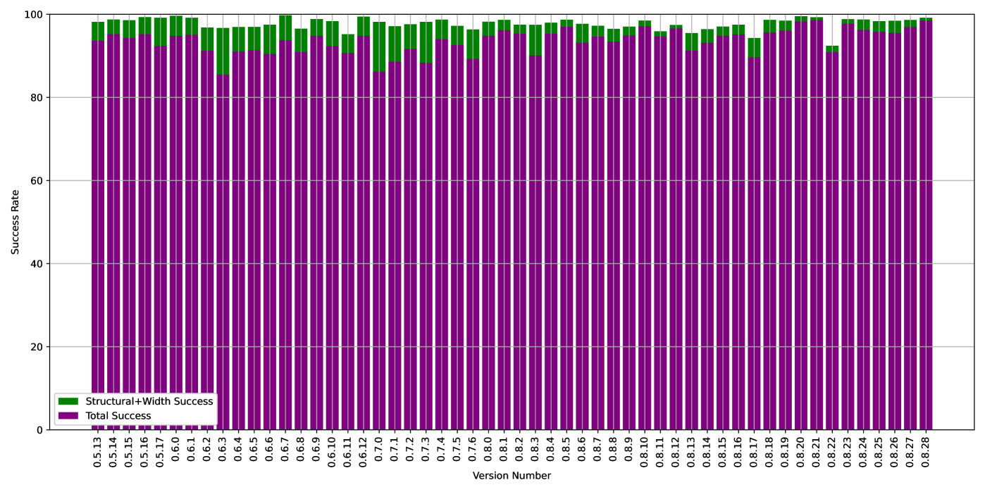
Figure 16. Success Rates for different compiler versions

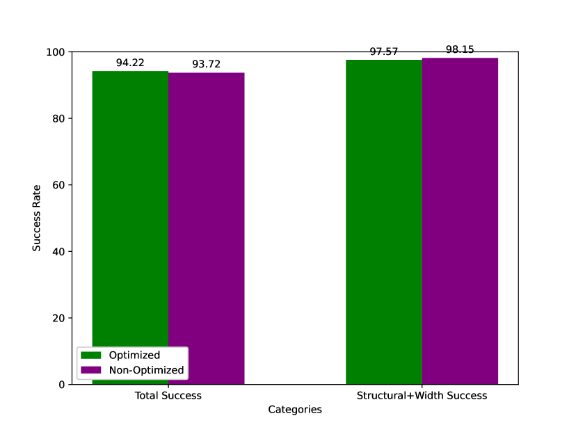
Figure 17. Success Rates for different compiler configurations

Figures 16 and 17 plot our precision metrics for the different compiler versions and optimization options of our dataset. These plots show that dyels’s performance is consistent regardless of compiler version and configuration.

7.3. Completeness

We evaluate the completeness of dyels by examining its ability to recover the ground truth, i.e., the recall of the analysis: the percentage of variables in the ground truth that dyels recovers. Table 4 shows the recall of the dyels inference to be around 92% for inferring structure+width and 88.50% for also inferring a correct unique type.

However, this number is only a lower bound.

The reason is that real-world smart contracts often need to declare unused variables. These variables are available to the compiler’s ground truth (since the compiler has access to the source code) but cannot be detected by any bytecode-level analysis. (Inferring these unused variables is a no-op for all practical purposes.)

The principal case of contracts that declare unused variables is upgradable proxy contracts. Upgradable proxy contracts need to maintain backwards compatibility of their storage layouts throughout their upgrades. (Failure to do this can result in storage collisions, a well-recognized problem, also studied in past literature (Ruaro et al., 2024).) The need to maintain compatible storage layouts makes developers continue to declare variables that are no longer used. Additionally, to avoid storage collisions, developers (and standard upgradability libraries) preemptively declare unused static arrays in storage, in order to keep a distance between the variables of a Solidity contract and those of the sub-contracts that inherit from it, so that future versions of the super-contract can add more variables.

One can observe from Table 4 that the majority of the incompleteness comes from 1898 (5.93%) instances of variables present in the ground truth but missed by dyels. We manually inspected 50 randomly-selected instances of such variables missed by dyels. Of these, 49 are unused variables, while one is a truly used variable that dyels misses due to incompleteness of the underlying EVM “memory” analysis. Our sampling has a margin of error of 13.86% for a confidence level of 95%. That is, with 95% confidence dyels misses at most 301 variables for the contracts in our dataset, with the rest of the 1597 reported missing variables being unused ones. Based on the above, the ground truth includes 30426 variables instead of the 32023 reported by solc.

Thus, with 95% confidence, the real recall of dyels is at least 96.77% for structure+width success and 93.14% for total success.

Yet another way to appreciate the completeness of dyels is by comparing the analysis recall to that of VarLifter. Table 5 shows the recall results for both tools, on the subset of contracts analyzed by both. dyels has a significantly higher recall than VarLifter, successfully identifying the structure+width of (at least) 92.58% of declared contract variables, and also the types of (at least) 89.38%. VarLifter is able to identify the structure+width of just 68.21% of declared variables and their correct, unique type in 67.46% of the cases.

The incompleteness of VarLifter is due to its incomplete path extraction algorithm that will not attempt to visit all code paths. In contrast, the dyels analysis is recursive to arbitrary depth, yet fully scalable—e.g., avoiding non-termination issues via the subtle treatment described in Section 5.1.2.

Furthermore, VarLifter’s implementation is heavily limited in terms of supported structures and the degrees of their composability:

• Nested mappings can only have a maximum depth of 2.

• Nested static arrays can only have at most 2 dimensions.

• Only value type and string arrays are supported.

• Only structs with members of value types are supported for mapping values. (Whereas storage slots of struct types may also contain strings.)

In contrast, the dyels inference algorithm of Section 5 is capable of detecting arbitrarily-nested storage structures.

7.4. Incompleteness in the compiler-produced metadata

As discussed in Section 3, common low-level storage patterns are not included in the compiler-produced storageLayout json. Therefore, dyels often retrieves more storage variables than the compiler itself. Of course, the compiler misses these variables because of the use of inline assembly. However, the inline assembly information is still available to the compiler, and certainly in much more accessible form than that available to a bytecode-only analyzer.

To quantify the impact, we measure the storage variables identified by dyels that are not present in the compiler-produced metadata. There are 268 missed storage variables in 213 contracts of our dataset. We warn that these numbers may be an overestimate, since multiple low-level variables can be a function of the same conceptual storage variable. (For example the index to access mapping element isAdmin[0xab5801a7d398351b8be11c439e05c5b3259aec9b] would be resolved to the result of keccak256(pad32(0xab5801a7d398351b8be11c439e05c5b3259aec9b), pad32(0x3)). Our analysis, unable to reverse the keccak hash, would include this as a boolean variable at index b3680c8d57306e73ce035d881dbc74713ad71f752db6726880df712cecb21733. This would appear separate from the mapping isAdmin itself, or other instances of variables similarly derived from it.)

We have not quantified exhaustively how many of the above inferred variables are separate variables in the smart contract code. However, our informal sampling suggests that a clear majority (over three-quarters) of contracts reported by dyels to be missing variables in the compiler-produced metadata, truly exhibit that behavior.

With this caveat in mind, we note that the number of affected contracts (213) is large, at 7.89% of the contracts in the dataset, reflecting a significant amount of incompleteness in compiler metadata. This is due to the use of the pattern of Section 3 in highly-adopted standards.

8. Related Work

Reasoning about the usage of the EVM’s storage has been instrumental for analysis tools and decompilers. However, no past tools (other than VarLifter—extensively compared earlier) attempt to statically fully recover storage structures as-if in the source program. For instance, past analyses may have inferred “this is an access to the balances mapping” but not the width of an entry, the full nested structure of the mapping, or the type of elements. Such work, discussed next, can potentially benefit from our techniques.

Most early frameworks (Albert et al., 2018; Tsankov et al., 2018) would only precisely reason about storage loading / storing statements with indexes resolved to constant values, sacrificing precision or completeness in low-level code treating dynamic data structures. Madmax (Grech et al., 2018) was the first work to propose an analysis that inferred high-level structures (arrays and mappings) from low-level EVM bytecode. This analysis enabled MadMax to detect storage-related vulnerabilities focusing on griefing and DoS. Ethainter (Brent et al., 2020) also made use of the storage modeling introduced in (Grech et al., 2018) to detect guarding patterns and track the propagation of taint through storage. An implicit modeling of storage was also achieved (as keccak256 expressions with free variables) in (Smaragdakis et al., 2021).

The recent CRUSH tool  (Ruaro et al., 2024) implements a storage collision vulnerability analysis for upgradable proxy contracts. Part of this work involves modeling storage, including a modeling of mappings, arrays, and byte-ranges of constant-offset storage slots to discriminate between storage variables packed into a single slot. Unfortunately, the work lacks support for arbitrarily-nested data structures. These same techniques have been applied (for the same security application) to the Proxion tool (Chen et al., 2024a). Another recent tool (Albert et al., 2024) analyzes storage access patterns to precisely compute the gas bounds of contracts via a Max-SMT based approach.

Other work has focused on analyzing the usage patterns of the EVM’s various “memory” stores. (Lagouvardos et al., 2020) proposes techniques to infer high-level facts from EVM bytecode. These inferences include high-level uses of operations reading from memory (hashing operations, external calls) memory arrays and their uses. dyels relies on these inferences for the modeling of the storage index values, and the propagation of type constraints through memory. The Certora prover employs a memory splitting transformation (Grossman et al., 2024) after modeling the allocations of high-level arrays and structs of EVM contracts and the aliasing between different allocations. This transformation allows the tool to consider disjoint memory locations separately, speeding up SMT queries by up to 120x. In other work (Albert et al., 2023) the uses of memory are analyzed to identify optimization opportunities.

Several other end-to-end applications rely on storage modeling. Storage modeling is also used in blockchain explorers and can be done dynamically. The leading storage explorer tool, evm.storage, uses such a dynamic analysis, by examining the use of hash pre-images derived from past executions of the contract. Analysis of confused deputy attack contracts has employed both static and dynamic storage modeling techniques (Gritti et al., 2023). A smart contract policy enforcer, EVM-Shield, utilizes storage modeling to pinpoint functions that perform state updates and adds pre- and post-conditions within the smart contract itself to prevent malicious transactions on-chain (Zhang et al., 2024).

Related to our work, past tools (Chen et al., 2021; Zhao et al., 2023) have been proposed to infer the ABI interfaces of unknown contracts by inferring the structures and types of public function arguments. Such tools can benefit from our work by taking our inferences into account in their type recovery efforts. As an example, SigRec (Chen et al., 2021), lacking a model of the EVM’s storage, considers any variable read from or written to storage to be of type uint256.

Outside the domain of smart contracts, a number of techniques on variable recognition and type inference of binaries are relevant to our work  (Lee et al., 2011; Caballero and Lin, 2016; Chen et al., 2020; Schwartz et al., 2018; Lehmann and Pradel, 2022; ElWazeer et al., 2013; Mycroft, 1999; Balakrishnan and Reps, 2007; Dolgova and Chernov, 2009). Static-analysis-based approaches (Mycroft, 1999; Balakrishnan and Reps, 2007; Ramalingam et al., 1999) have historically seen widespread adoption in this setting. Recent learning-based tools (Song et al., 2024; Maier et al., 2019; Pei et al., 2021) have also been successful in recovering type information from binaries. More closely related to our approach, OOAnalyzer (Schwartz et al., 2018) uses Prolog to infer C++ classes from binaries.

9. Conclusion

We presented dyels, a static-analysis-based lifter for storage variables from the binaries of Ethereum smart contracts. dyels, powered by an analysis of low-level storage indexes, is able to resolve arbitrarily-nested high-level data structures from the low-level bytecode. Compared against the state-of-the-art in a diverse dataset of real-world contracts, dyels manages to excel in all evaluation dimensions: scalability, precision, and completeness, even inferring variables missing in the compiler-produced metadata.

References

- (1)
- Albert et al. (2023) Elvira Albert, Jesús Correas, Pablo Gordillo, Guillermo Román-Díez, and Albert Rubio. 2023. Inferring Needless Write Memory Accesses on Ethereum Bytecode. In Tools and Algorithms for the Construction and Analysis of Systems, Sriram Sankaranarayanan and Natasha Sharygina (Eds.). Springer Nature Switzerland, Cham, 448–466.
- Albert et al. (2024) Elvira Albert, Jesús Correas, Pablo Gordillo, Guillermo Román-Díez, and Albert Rubio. 2024. Synthesis of Sound and Precise Storage Cost Bounds via Unsound Resource Analysis and Max-SMT. In Proceedings of the 33rd ACM SIGSOFT International Symposium on Software Testing and Analysis (Vienna, Austria) (ISSTA 2024). Association for Computing Machinery, New York, NY, USA, 1186–1197. https://doi.org/10.1145/3650212.3680352
- Albert et al. (2018) Elvira Albert, Pablo Gordillo, Benjamin Livshits, Albert Rubio, and Ilya Sergey. 2018. EthIR: A Framework for High-Level Analysis of Ethereum Bytecode. In Automated Technology for Verification and Analysis, Shuvendu K. Lahiri and Chao Wang (Eds.). Springer International Publishing, Cham, 513–520.
- Balakrishnan and Reps (2007) Gogul Balakrishnan and Thomas Reps. 2007. DIVINE: DIscovering Variables IN Executables. In Verification, Model Checking, and Abstract Interpretation, Byron Cook and Andreas Podelski (Eds.). Springer Berlin Heidelberg, Berlin, Heidelberg, 1–28.
- Becker (2023) Jonathan Becker. 2023. Heimdall is an advanced EVM smart contract toolkit specializing in bytecode analysis and extracting information from unverified contracts. https://github.com/Jon-Becker/heimdall-rs
- Brent et al. (2020) Lexi Brent, Neville Grech, Sifis Lagouvardos, Bernhard Scholz, and Yannis Smaragdakis. 2020. Ethainter: A Smart Contract Security Analyzer for Composite Vulnerabilities. In Proceedings of the 41st ACM SIGPLAN Conference on Programming Language Design and Implementation (London, UK) (PLDI 2020). Association for Computing Machinery, New York, NY, USA, 454–469. https://doi.org/10.1145/3385412.3385990
- Caballero and Lin (2016) Juan Caballero and Zhiqiang Lin. 2016. Type Inference on Executables. ACM Comput. Surv. 48, 4, Article 65 (May 2016), 35 pages. https://doi.org/10.1145/2896499
- Chaliasos et al. (2022) Stefanos Chaliasos, Arthur Gervais, and Benjamin Livshits. 2022. A study of inline assembly in solidity smart contracts. Proc. ACM Program. Lang. 6, OOPSLA2, Article 165 (Oct. 2022), 27 pages. https://doi.org/10.1145/3563328
- Chen et al. (2024a) Cheng-Kang Chen, Wen-Yi Chu, Muoi Tran, Laurent Vanbever, and Hsu-Chun Hsiao. 2024a. Proxion: Uncovering Hidden Proxy Smart Contracts for Finding Collision Vulnerabilities in Ethereum. arXiv:2409.13563 [cs.CR] https://arxiv.org/abs/2409.13563
- Chen et al. (2020) Ligeng Chen, Zhongling He, and Bing Mao. 2020. CATI: Context-Assisted Type Inference from Stripped Binaries. In 2020 50th Annual IEEE/IFIP International Conference on Dependable Systems and Networks (DSN). 88–98. https://doi.org/10.1109/DSN48063.2020.00028
- Chen et al. (2021) Ting Chen, Zihao Li, Xiapu Luo, Xiaofeng Wang, Ting Wang, Zheyuan He, Kezhao Fang, Yufei Zhang, Hang Zhu, Hongwei Li, Yan Cheng, and Xiao-song Zhang. 2021. SigRec: Automatic Recovery of Function Signatures in Smart Contracts. IEEE Transactions on Software Engineering (2021), 1–1. https://doi.org/10.1109/TSE.2021.3078342
- Chen et al. (2024b) Zhiyang Chen, Ye Liu, Sidi Mohamed Beillahi, Yi Li, and Fan Long. 2024b. Demystifying Invariant Effectiveness for Securing Smart Contracts. Proc. ACM Softw. Eng. 1, FSE, Article 79 (July 2024), 24 pages. https://doi.org/10.1145/3660786
- Dolgova and Chernov (2009) E. N. Dolgova and A. V. Chernov. 2009. Automatic reconstruction of data types in the decompilation problem. Program. Comput. Softw. 35, 2 (March 2009), 105–119. https://doi.org/10.1134/S0361768809020066
- ElWazeer et al. (2013) Khaled ElWazeer, Kapil Anand, Aparna Kotha, Matthew Smithson, and Rajeev Barua. 2013. Scalable variable and data type detection in a binary rewriter. SIGPLAN Not. 48, 6 (June 2013), 51–60. https://doi.org/10.1145/2499370.2462165
- etherscan.io (2017) etherscan.io. 2017. Etherscan Blockchain explorer. https://etherscan.io
- Grech et al. (2019) Neville Grech, Lexi Brent, Bernhard Scholz, and Yannis Smaragdakis. 2019. Gigahorse: Thorough, Declarative Decompilation of Smart Contracts. In Proceedings of the 41st International Conference on Software Engineering (Montreal, Quebec, Canada) (ICSE ’19). IEEE Press, Piscataway, NJ, USA, 1176–1186. https://doi.org/10.1109/ICSE.2019.00120
- Grech et al. (2018) Neville Grech, Michael Kong, Anton Jurisevic, Lexi Brent, Bernhard Scholz, and Yannis Smaragdakis. 2018. MadMax: Surviving Out-of-Gas Conditions in Ethereum Smart Contracts. Proc. ACM Programming Languages 2, OOPSLA (Nov. 2018). https://doi.org/10.1145/3276486
- Grech et al. (2022) Neville Grech, Sifis Lagouvardos, Ilias Tsatiris, and Yannis Smaragdakis. 2022. Elipmoc: advanced decompilation of Ethereum smart contracts. Proc. ACM Program. Lang. 6, OOPSLA1, Article 77 (apr 2022), 27 pages. https://doi.org/10.1145/3527321
- Gritti et al. (2023) Fabio Gritti, Nicola Ruaro, Robert McLaughlin, Priyanka Bose, Dipanjan Das, Ilya Grishchenko, Christopher Kruegel, and Giovanni Vigna. 2023. Confusum Contractum: Confused Deputy Vulnerabilities in Ethereum Smart Contracts. In 32nd USENIX Security Symposium (USENIX Security 23). USENIX Association, Anaheim, CA, 1793–1810. https://www.usenix.org/conference/usenixsecurity23/presentation/gritti
- Grossman et al. (2024) Shelly Grossman, John Toman, Alexander Bakst, Sameer Arora, Mooly Sagiv, and Chandrakana Nandi. 2024. Practical Verification of Smart Contracts using Memory Splitting. Proc. ACM Program. Lang. 8, OOPSLA2, Article 356 (Oct. 2024), 32 pages. https://doi.org/10.1145/3689796
- Hu et al. (2021) Xiaowen Hu, David Zhao, Herbert Jordan, and Bernhard Scholz. 2021. An efficient interpreter for Datalog by de-specializing relations. In Proceedings of the 42nd ACM SIGPLAN International Conference on Programming Language Design and Implementation (Virtual, Canada) (PLDI 2021). Association for Computing Machinery, New York, NY, USA, 681–695. https://doi.org/10.1145/3453483.3454070
- Jordan et al. (2016) Herbert Jordan, Bernhard Scholz, and Pavle Subotić. 2016. Soufflé: On Synthesis of Program Analyzers. In Computer Aided Verification, Swarat Chaudhuri and Azadeh Farzan (Eds.). Springer International Publishing, Cham, 422–430.
- Kolinko and Palkeo (2020) Tomasz Kolinko and Palkeo. 2020. Panoramix – Decompiler at the heart of eveem.org. https://github.com/palkeo/panoramix
- Lagouvardos et al. (2020) Sifis Lagouvardos, Neville Grech, Ilias Tsatiris, and Yannis Smaragdakis. 2020. Precise Static Modeling of Ethereum “Memory”. Proc. ACM Program. Lang. 4, OOPSLA, Article 190 (nov 2020), 26 pages. https://doi.org/10.1145/3428258
- Lee et al. (2011) JongHyup Lee, Thanassis Avgerinos, and David Brumley. 2011. TIE: Principled reverse engineering of types in binary programs. In 18th Annual Network and Distributed System Security Symposium (NDSS’11).
- Lehmann and Pradel (2022) Daniel Lehmann and Michael Pradel. 2022. Finding the Dwarf: Recovering Precise Types from WebAssembly Binaries. In Proceedings of the 43rd ACM SIGPLAN International Conference on Programming Language Design and Implementation (San Diego, CA, USA) (PLDI 2022). Association for Computing Machinery, New York, NY, USA, 410–425. https://doi.org/10.1145/3519939.3523449
- Li et al. (2024) Yichuan Li, Wei Song, and Jeff Huang. 2024. VarLifter: Recovering Variables and Types from Bytecode of Solidity Smart Contracts. Proc. ACM Program. Lang. 8, OOPSLA2, Article 271 (Oct. 2024), 29 pages. https://doi.org/10.1145/3689711
- Maier et al. (2019) Alwin Maier, Hugo Gascon, Christian Wressnegger, and Konrad Rieck. 2019. TypeMiner: Recovering Types in Binary Programs Using Machine Learning. In Detection of Intrusions and Malware, and Vulnerability Assessment, Roberto Perdisci, Clémentine Maurice, Giorgio Giacinto, and Magnus Almgren (Eds.). Springer International Publishing, Cham, 288–308.
- Mycroft (1999) Alan Mycroft. 1999. Type-Based Decompilation (or Program Reconstruction via Type Reconstruction). In Programming Languages and Systems, S. Doaitse Swierstra (Ed.). Springer Berlin Heidelberg, Berlin, Heidelberg, 208–223.
- Palladino et al. (2019) Santiago Palladino, Francisco Giordano, and Hadrien Croubois. 2019. ERC-1967: Proxy Storage Slots. https://eips.ethereum.org/EIPS/eip-1967
- Pei et al. (2021) Kexin Pei, Jonas Guan, Matthew Broughton, Zhongtian Chen, Songchen Yao, David Williams-King, Vikas Ummadisetty, Junfeng Yang, Baishakhi Ray, and Suman Jana. 2021. StateFormer: fine-grained type recovery from binaries using generative state modeling. In Proceedings of the 29th ACM Joint Meeting on European Software Engineering Conference and Symposium on the Foundations of Software Engineering (Athens, Greece) (ESEC/FSE 2021). Association for Computing Machinery, New York, NY, USA, 690–702. https://doi.org/10.1145/3468264.3468607
- Ramalingam et al. (1999) G. Ramalingam, John Field, and Frank Tip. 1999. Aggregate structure identification and its application to program analysis. In Proceedings of the 26th ACM SIGPLAN-SIGACT Symposium on Principles of Programming Languages (San Antonio, Texas, USA) (POPL ’99). Association for Computing Machinery, New York, NY, USA, 119–132. https://doi.org/10.1145/292540.292553
- Ruaro et al. (2024) Nicola Ruaro, Fabio Gritti, Robert McLaughlin, Ilya Grishchenko, Christopher Kruegel, and Giovanni Vigna. 2024. Not your Type! Detecting Storage Collision Vulnerabilities in Ethereum Smart Contracts. (2024).
- Scholz et al. (2016) Bernhard Scholz, Herbert Jordan, Pavle Subotic, and Till Westmann. 2016. On fast large-scale program analysis in Datalog. In Proceedings of the 25th International Conference on Compiler Construction, CC 2016, Barcelona, Spain, March 12-18, 2016, Ayal Zaks and Manuel V. Hermenegildo (Eds.). ACM, 196–206. https://doi.org/10.1145/2892208.2892226
- Schwartz et al. (2018) Edward J. Schwartz, Cory F. Cohen, Michael Duggan, Jeffrey Gennari, Jeffrey S. Havrilla, and Charles Hines. 2018. Using Logic Programming to Recover C++ Classes and Methods from Compiled Executables. In Proceedings of the 2018 ACM SIGSAC Conference on Computer and Communications Security (Toronto, Canada) (CCS 18). Association for Computing Machinery, New York, NY, USA, 426–441. https://doi.org/10.1145/3243734.3243793
- Smaragdakis et al. (2021) Yannis Smaragdakis, Neville Grech, Sifis Lagouvardos, Konstantinos Triantafyllou, and Ilias Tsatiris. 2021. Symbolic Value-Flow Static Analysis: Deep, Precise, Complete Modeling of Ethereum Smart Contracts. Proc. ACM Program. Lang. 5, OOPSLA, Article 163 (oct 2021), 30 pages. https://doi.org/10.1145/3485540
- Solidity Team (2019) Solidity Team. 2019. Solidity 0.5.13 Release Announcement. https://soliditylang.org/blog/2019/11/14/solidity-0.5.13-release-announcement/
- Solidity Team (2024) Solidity Team. 2024. Solidity 0.8.28 Release Announcement. https://soliditylang.org/blog/2024/10/09/solidity-0.8.28-release-announcement/
- Song et al. (2024) Zirui Song, YuTong Zhou, Shuaike Dong, Ke Zhang, and Kehuan Zhang. 2024. TypeFSL: Type Prediction from Binaries via Inter-procedural Data-flow Analysis and Few-shot Learning. In Proceedings of the 39th IEEE/ACM International Conference on Automated Software Engineering (Sacramento, CA, USA) (ASE ’24). Association for Computing Machinery, New York, NY, USA, 1269–1281. https://doi.org/10.1145/3691620.3695502
- Tsankov et al. (2018) Petar Tsankov, Andrei Dan, Dana Drachsler-Cohen, Arthur Gervais, Florian Bünzli, and Martin Vechev. 2018. Securify: Practical Security Analysis of Smart Contracts. In Proceedings of the 2018 ACM SIGSAC Conference on Computer and Communications Security (Toronto, Canada) (CCS ’18). ACM, New York, NY, USA, 67–82. https://doi.org/10.1145/3243734.3243780
- Werner et al. (2023) Sam Werner, Daniel Perez, Lewis Gudgeon, Ariah Klages-Mundt, Dominik Harz, and William Knottenbelt. 2023. SoK: Decentralized Finance (DeFi). In Proceedings of the 4th ACM Conference on Advances in Financial Technologies (Cambridge, MA, USA) (AFT ’22). Association for Computing Machinery, New York, NY, USA, 30–46. https://doi.org/10.1145/3558535.3559780
- Yang et al. (2024) Shuo Yang, Xingwei Lin, Jiachi Chen, Qingyuan Zhong, Lei Xiao, Renke Huang, Yanlin Wang, and Zibin Zheng. 2024. Hyperion: Unveiling DApp Inconsistencies using LLM and Dataflow-Guided Symbolic Execution. arXiv:2408.06037 [cs.SE] https://arxiv.org/abs/2408.06037
- Zhang et al. (2024) Xiaoli Zhang, Wenxiang Sun, Zhicheng Xu, Hongbing Cheng, Chengjun Cai, Helei Cui, and Qi Li. 2024. EVM-Shield: In-Contract State Access Control for Fast Vulnerability Detection and Prevention. IEEE Transactions on Information Forensics and Security 19 (2024), 2517–2532. https://doi.org/10.1109/TIFS.2024.3349852
- Zhao et al. (2023) Kunsong Zhao, Zihao Li, Jianfeng Li, He Ye, Xiapu Luo, and Ting Chen. 2023. DeepInfer: Deep Type Inference from Smart Contract Bytecode. In Proceedings of the 31st ACM Joint European Software Engineering Conference and Symposium on the Foundations of Software Engineering (San Francisco, CA, USA) (ESEC/FSE 2023). Association for Computing Machinery, New York, NY, USA, 745–757. https://doi.org/10.1145/3611643.3616343