Low-Energy Constants of Chiral Perturbation Theory from Pion Scalar Form Factors in $N_{f}=2+1$-Flavor Lattice QCD with Controlled Errors

Abstract

We determine the low-energy constants (LECs) $f_{0}$, $L_{4}^{r}$ and $L_{5}^{r}$ of SU(3) Chiral Perturbation Theory ($\chi$PT) from a lattice QCD calculation of the scalar form factors of the pion with fully controlled systematics. Lattice results are computed on a large set of $N_{f}=2+1$ gauge ensembles covering four lattice spacings $a\in[0.049,0.086]\mathrm{fm}$, pion masses $M_{\pi}\in[130,350]\mathrm{MeV}$, and various large physical volumes. By determining the notorious quark-disconnected contributions with unprecedented precision and using a large range of source-sink separations $t_{\mathrm{sep}}\in[1.0,3.25]\,\mathrm{fm}$, we are able for the first time to obtain the scalar radii from a $z$-expansion parameterization of the form factors rather than a simple linear approximation at small momentum transfer. The LECs are obtained from the physical extrapolation of the radii using NLO SU(3) NLO $\chi$PT to parameterize the quark mass dependence. Systematic uncertainties are estimated via model averages based on the Akaike Information Criterion. Our determination of $L_{4}^{r}$ is the first lattice determination to obtain a result not compatible with zero.

I Introduction

Quark-hadron duality implies that one can study low-energy hadron physics via two different approaches, either on the phenomenological level of hadrons using effective theories such as in Chiral Perturbation Theory ($\chi$PT), or on the fundamental level of quarks and gluons using non-perturbative Quantum Chromodynamics (QCD), in particular lattice QCD simulations.

Historically, $\chi$PT has been an indispensable tool for lattice QCD practitioners, who required it to extrapolate results from lattice simulations performed using unphysically heavy quark masses to the physical quark mass point. Nowadays, however, the relationship between $\chi$PT and lattice QCD has changed, since algorithmic improvements and the progress of computer technology have enabled simulations directly at physical quark masses. Now it is lattice QCD with its ability to simulate at unphysical values of the quark masses that can offer added value to $\chi$PT by extracting values for its low-energy constants (LECs) from first principles.

Of particular interest in this context are quantities depending only on a single or very fery LECs. An example of such quantities are the scalar radii

$$\langle r^{2}_{S}\rangle_{\pi}^{f}=\left.-\frac{6}{F_{S}^{\pi,f}(0)}\frac{dF_{S}^{\pi,f}(Q^{2})}{dQ^{2}}\right|_{Q^{2}\rightarrow 0}$$ (1)

that parameterize the scalar form factors

$$F^{\pi,f}_{S}(Q^{2})=\left\langle\pi(\mathbf{p}_{f})\right|\mathcal{S}^{f}\left|\pi(\mathbf{p}_{i})\right\rangle$$ (2)

at low values of $Q^{2}=-q^{2}=-(p_{f}-p_{i})^{2}$. In the $N_{f}=2$ theory, the only isoscalar scalar density is the light one,

$$\mathcal{S}^{l}=\bar{u}u+\bar{d}d\,,$$ (3)

and in $\mathrm{SU}\left(2\right)$ $\chi$PT, the corresponding scalar radius depends only on $\bar{\ell}_{4}$ via

$$\langle r^{2}_{S}\rangle_{\pi}^{l}=\frac{1}{8\pi^{2}f_{\pi,\mathrm{phys}}^{2}}\left[-\frac{13}{2}+\bar{\ell}_{4}+\log\frac{M_{\pi,\mathrm{phys}}^{2}}{M_{\pi}^{2}}\right].$$ (4)

With $N_{f}=2+1$ quark flavors, the scalar densities can be expressed in the basis of the singlet and octet ones,

$$\mathcal{S}^{0} =\bar{u}u+\bar{d}d-2\bar{s}s\,,$$ (5)

$$\mathcal{S}^{8} =\bar{u}u+\bar{d}d+\bar{s}s\,,$$ (6)

and in $\mathrm{SU}\left(3\right)$ $\chi$PT, the scalar radii are related by [1]

$$\langle r^{2}_{S}\rangle_{\pi}^{0} =\langle r^{2}_{S}\rangle_{\pi}^{8}+\delta r^{2}_{S},$$ (7)

$$\langle r^{2}_{S}\rangle_{\pi}^{l} =\langle r^{2}_{S}\rangle_{\pi}^{8}+\frac{2}{3}\delta r^{2}_{S},$$ (8)

where the octet radius depends only on $L_{5}^{r}$, while the singlet and light radii depend on both $L_{5}^{r}$ and $L_{4}^{r}$.

The LECs $\bar{\ell}_{4}$, and $L_{5}^{r}$ and $L_{4}^{r}$ can therefore be accurately determined from a high-precision determination of the scalar form factors.

In this letter, we present a high-statistics determination of the scalar form factors with fully controlled systematics, including the extrapolation to the physical point. The use of moving frames allows us to achieve far better momentum resolution than previous studies, and we determine the numerically challenging quark-disconnected with a statistical precision that is more than an order of magnitude better than the best preceding determination, resulting in the first lattice determination of $L_{4}^{r}$ that is not compatible with zero.

II Setup

The lattice calculation of the scalar form factors has been carried out on a set of 17 gauge ensembles produced by the Coordinated Lattice Simulations (CLS) consortium [2] using $N_{f}=2+1$ flavors of non-perturbatively $\mathcal{O}(a)$-improved Wilson fermions [3] and a tree-level Symanzik-improved gauge action [4]. The majority of the ensembles use open boundary conditions in time to mitigate topological freezing [5, 6], whereas some ensembles use periodic boundary conditions. Due to the use of a twisted-mass regulator [6] for the light quarks and a rational approximation for the strange quark [7], reweighting factors [8, 2, 9] have to be applied when taking gauge averages.

Most of the ensembles lie on the chiral trajectory defined by $\mathrm{tr}[M]=2m_{l}+m_{s}=\mathrm{const}$, but additional ensembles on a second chiral trajectory defined by $m_{s}\approx m_{s}^{\mathrm{phys}}$ have been included in order to provide a better handle on the separate $m_{l}$ and $m_{s}$ dependence in the chiral extrapolations.

Scale setting is performed via the gradient flow scale $t_{0}$ [10], using the values for $t_{0}^{\mathrm{sym}}/a^{2}$ at the symmetrical point from Ref. [11], while defining the physical light and strange quark masses using the $N_{f}=2+1$ FLAG world average [12]

$$\sqrt{t_{0}^{\mathrm{phys}}}=0.14464(87)\,\mathrm{fm}\,,$$ (9)

The matrix elements in Eq. (2) are evaluated in lattice QCD by taking the ratio

$$R^{f}(\mathfrak{p}_{f},\mathfrak{q},\mathfrak{p}_{i},t_{\mathrm{sep}},t_{\mathrm{ins}})=\frac{\langle C_{P\mathcal{S}^{f}P}^{\mathrm{3pt}}(\mathfrak{p}_{f},\mathfrak{q},\mathfrak{p}_{i},t_{\mathrm{sep}},t_{\mathrm{ins}})\rangle}{\langle C_{PP}^{\mathrm{2pt}}(\mathfrak{p}_{f},t_{\mathrm{sep}})\rangle}$$ (10)

$$\times\sqrt{\frac{\langle C_{PP}^{\mathrm{2pt}}(\mathfrak{p}_{i},t_{\mathrm{sep}}-t_{\mathrm{ins}})\rangle\langle C_{PP}^{\mathrm{2pt}}(\mathfrak{p}_{f}^{2},t_{\mathrm{ins}})\rangle\langle C_{PP}^{\mathrm{2pt}}(\mathfrak{p}_{f}^{2},t_{\mathrm{sep}})\rangle}{\langle C_{PP}^{\mathrm{2pt}}(\mathfrak{p}_{f}^{2},t_{\mathrm{sep}}-t_{\mathrm{ins}})\rangle\langle C_{PP}^{\mathrm{2pt}}(\mathfrak{p}_{i}^{2},t_{\mathrm{ins}})\rangle\langle C_{PP}^{\mathrm{2pt}}(\mathfrak{p}_{i}^{2},t_{\mathrm{sep}})\rangle}}\,,$$

of the two- and three-point functions

$$C_{PP}^{\mathrm{2pt}}(\mathbf{p},t) =\sum_{\mathbf{x}_{f}}e^{i\mathbf{p}\cdot\mathbf{x}_{f}}\left<P(\mathbf{x}_{f},t)P^{\dagger}(\mathbf{0},0)\right>_{F}\,,$$ (11)

$$C_{P\mathcal{S}^{f}P}^{\mathrm{3pt}}(\mathbf{p}_{f},\mathbf{q},t_{\mathrm{sep}},t_{\mathrm{ins}}) =\sum_{\mathbf{x}_{f},\mathbf{x}_{op}}e^{i\mathbf{p}_{f}\cdot\mathbf{x}_{f}}e^{i\mathbf{q}\cdot\mathbf{x}_{op}}\times$$ (12)

$$\left<P(\mathbf{x}_{f},t_{\mathrm{sep}})\mathcal{S}^{f}(\mathbf{x}_{op},t_{\mathrm{ins}})P^{\dagger}(\mathbf{0},0)\right>_{F}\,,$$

where $P(\mathbf{x},t)=\frac{1}{\sqrt{2}}\left[\bar{u}\gamma_{5}u+\bar{d}\gamma_{5}d\right](\mathbf{x},t)$, and $\left(\mathfrak{p}_{f},\mathfrak{q},\mathfrak{p}_{i}\right)$ are equivalence classes of lattice momenta $(\mathbf{p}_{f},\mathbf{q},\mathbf{p}_{i})$ over which the correlation functions have been averaged.

Performing the Wick contractions for the fermionic expectation value $\langle\cdot\rangle_{F}$ in the three-point function in Eq. (12) yields both quark-connected and quark-disconnected diagrams. The quark-connected piece is computed to high statistical precision using a sequential propagator through the sink [13] and the truncated solver method (TSM) [14, 15, 16]. The numerical evaluation of the quark-disconnected contribution requires correlating two-point functions $C_{PP}^{\mathrm{2pt}}(\mathbf{p}_{f},t)$ with scalar quark loops

$$L_{\mathcal{S}^{f}}(\mathbf{q},t)=-\sum\limits_{\mathbf{x}}e^{i\mathbf{q}\cdot\mathbf{x}}\mathrm{tr}\left[D_{f}^{-1}(x,x)\right]\,,$$ (13)

where $D_{f}$ is the Dirac operator for quark flavor $f=l,s$. These loops have been calculated using the (OET+gHPE+HP) prescription we introduced in Ref. [17] on the basis of the method of Ref. [18], combining the one-end trick (OET) [19] with the generalized hopping parameter expansion (gHPE) [20] and hierarchical probing (HP) [21].

One final wrinkle concerns the estimation of the subtraction of the vacuum expectation value (vev) of the scalar loop at zero momentum. With open boundary conditions, the need to avoid the region close to the boundaries leads to restrictions on the source positions that can be used at a given $t_{\mathrm{sep}}$, which in turn leads to an amplification of fluctuations in the loop at large $t_{\mathrm{sep}}$, where few sources contribute to the two-point function. To cancel these fluctuations, we determine and subtract the vev on each timeslice separately, leading to a large improvement in signal quality.

III Data Analysis

For large time separations, the ratio (10) tends directly to the scalar form factor of the pion, $\lim_{t_{\mathrm{sep}}\gg t_{\mathrm{ins}}\to\infty}R^{f}(\mathfrak{p}_{f},\mathfrak{q},\mathfrak{p}_{i},t_{\mathrm{sep}},t_{\mathrm{ins}})=F_{S}^{\pi,f}(Q^{2})$. To extract the form factor at finite $t_{\mathrm{sep}}$, $t_{\mathrm{ins}}$, we use the summation method [22, 23, 24, 25]

$$\sum_{t_{\mathrm{ins}}=\tau}^{t_{\mathrm{sep}}-\tau}R^{f}(\mathfrak{p}_{f},\mathfrak{q},\mathfrak{p}_{i},t_{\mathrm{sep}},t_{\mathrm{ins}}) =C_{\tau}+t_{\mathrm{sep}}F_{S}^{\pi,f}(Q^{2})$$ (14)

$$+\mathcal{O}\left(e^{-\Delta t_{\mathrm{sep}}}\right)\,,$$

where $C_{\tau}$ is an irrelevant constant, and $\Delta$ is the energy gap between the first excited state and the ground state. We perform linear fits over different ranges $t_{\mathrm{sep}}\in\left[t_{\mathrm{sep}}^{\mathrm{min}},t_{\mathrm{sep}}^{\mathrm{max}}\right]$ of the summed ratio, where $1.0\,\mathrm{fm}\lesssim t_{\mathrm{sep}}^{\mathrm{min}}\lesssim 1.5\,\mathrm{fm}$ and $2.5\,\mathrm{fm}\lesssim t_{\mathrm{sep}}^{\mathrm{max}}\lesssim 3.0\,\mathrm{fm}$ on each ensemble, and $\tau=t_{\mathrm{sep}}^{\mathrm{min}}/2$.

We parameterize the $Q^{2}$-dependence of the resulting form factors using the $z$-expansion ansatz

$$F_{S}^{\pi,f}(Q^{2})=\sum_{n=0}^{N_{z}}a_{n}z^{n}\,,\quad z=\frac{\sqrt{t_{\mathrm{cut}}+Q^{2}}-\sqrt{\vphantom{Q^{2}}t_{\mathrm{cut}}-t_{\mathrm{opt}}}}{\sqrt{t_{\mathrm{cut}}+Q^{2}}+\sqrt{\vphantom{Q^{2}}t_{\mathrm{cut}}-t_{\mathrm{opt}}}}\,,$$ (15)

in terms of which the radii are given by

$$a_{1}\sim\langle r_{S}^{2}\rangle_{\pi}^{f}=-\frac{6}{F_{S}^{\pi,f}(0)}\cdot\left.\frac{dF_{S}^{\pi,f}(Q^{2})}{dQ^{2}}\right|_{Q^{2}=0}\,.$$ (16)

In our fits, which we perform for five different cuts $Q^{2}_{\mathrm{max}}\in\left[0.2,0.4\right]\,\mathrm{GeV}^{2}$ on $Q^{2}\leq Q^{2}_{\mathrm{max}}$, we always use $N_{z}=1$, $t_{\mathrm{cut}}=4M_{\pi}^{2}$, and $t_{\mathrm{opt}}=t_{\mathrm{cut}}(1-\sqrt{1+Q^{2}_{\mathrm{max}}/t_{\mathrm{cut}}})$ [26].

Examples of the form factors obtained are shown in Fig. 1. It can be clearly seen that the addition of moving frames greatly improves the precision of the data and allows fits out to much larger momentum transfers.

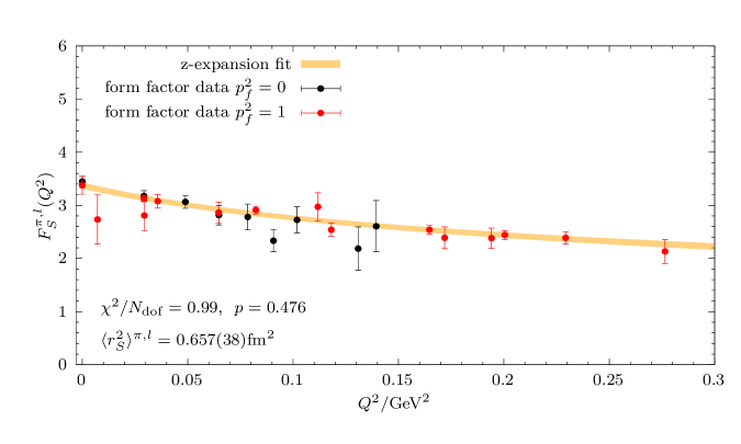
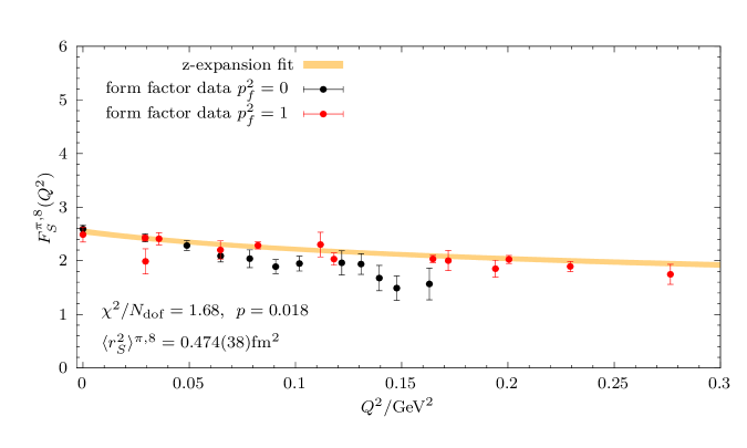
Figure 1: Form factor data (black for $\mathbf{p}_{f}^{2}=0$ and red for $\mathbf{p}_{f}^{2}=1$ frame) and $z$-expansion fit bands for $F_{S}^{\pi,l}(Q^{2})$ (top) and $F_{S}^{\pi,8}(Q^{2})$ (bottom) on the physical-mass ensemble E250. The results shown are for the data set with source-sink separations $t_{\mathrm{sep}}\in[1.25,3.25]\,\mathrm{fm}$ in the summation method, and a fit range $Q^{2}\leq 0.3\,\mathrm{GeV}^{2}$ for the $z$-expansion.

To extrapolate the scalar radii to the physical point, we use fit ansätze based on NLO $SU(3)$ $\chi$PT. To this end, we rewrite the expressions for $\langle r^{2}_{S}\rangle_{\pi}^{8}$ and $\delta r^{2}_{S}$ in terms of the leading-order quark-mass proxies $\xi_{l}=t_{0}M_{\pi}^{2}$ and $\xi_{s}=t_{0}(2M_{K}^{2}-M_{\pi}^{2})$, expressing all dimensionful observables in units of $t_{0}$ such that the scale-dependence $\mu$ is absorbed in the definitions of $L_{4,5}^{r}$, implicitly setting $\sqrt{t_{0}}\mu=1$ in the fits. We also include a term $\sim a^{2}/t_{0}$ to account for discretization effects. To account for finite-volume effects, we have also included the finite-volume corrections [27], but found that these tend to worsen the fit quality while having no significant impact on the central values due to our already rather large volumes.

While simultaneous fits for all three radii would in principle allow simultaneous access to all LECs, we find that the very strong correlations between the different radii render such fits problematic, resulting in typically unacceptable fit qualities. We therefore opt to fit suitable linear combinations that isolate $L_{4}^{r}$ and $L_{5}^{r}$.

We perform the entire analysis chain with different cuts on the range of $t_{\mathrm{sep}}$ used in the summation method, the range of $Q^{2}$ fitted in the $z$-expansion fit, and the values of $a$, $M_{\pi}$ and $M_{\pi}L$ included in the physical extrapolation. To arrive at our final best estimates including the full statistical and systematic errors, we perform a model average [28, 29] based on the Akaike Information Criterion (AIC) [30, 31] by computing weights

$$w_{n,b}=\frac{e^{-B_{n,b}}}{N_{B}\sum_{k=1}^{N_{M}}e^{-B_{k,b}}}$$ (17)

for model $n\in\{1,\ldots N_{M}\}$ on bootstrap resample $b\in\{1,\ldots,N_{B}\}$ with

$$B_{n,b}=\frac{1}{2}\chi^{2}_{n,b}+N_{\mathrm{par},n}+N_{\mathrm{cut},n}-N_{\mathrm{prio}}$$ (18)

where $\chi^{2}_{n,b}$ is the correlated $\chi^{2}$ for model $n$ on bootstrap resample $b$, and $N_{\mathrm{par},n}$ and $N_{\mathrm{cut},n}$ are the number of parameters in model $n$ and the number of data points cut for fitting with model $n$, respectively [31], while $N_{\mathrm{prio}}=1$ accounts for the (uninformative) prior applied to $f_{0}$ to stabilize the fits. Our empirical cumulative distribution function (CDF) is then

$$CDF(x)=\sum_{b=1}^{N_{B}}\sum_{n=1}^{N_{M}}w_{n,b}\Theta(x-x_{n,b})$$ (19)

where $x_{n,b}$ is the value of $x$ obtained from model $n$ on bootstrap sample $b$, and $\Theta$ is the Heaviside step function.

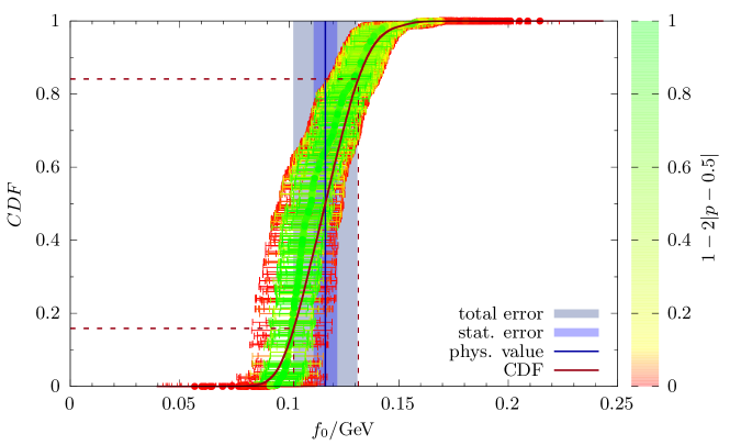
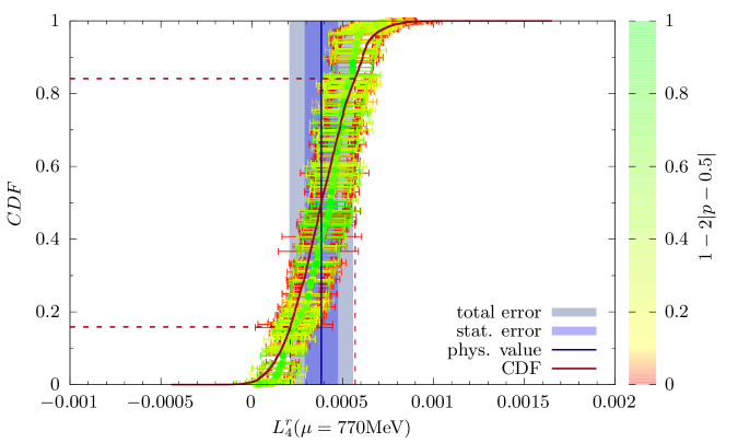
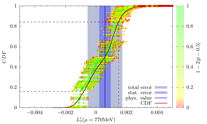
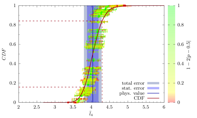
Figure 2: Cumulative distribution functions (CDFs) of the results for the $\mathrm{SU}\left(3\right)$ LECs $f_{0}$, $L_{4}^{r}(\mu)$ and $L_{5}^{r}(\mu)$ at a scale of $\mu=770\,\mathrm{MeV}$ and the $\mathrm{SU}\left(2\right)$ LEC $\bar{\ell}_{4}$. Each data point represents the result and statistical error from an individual fit model and its color is determined by the corresponding $p$-value indicating the quality of the fit (which is different from the Akaike weight actually used to obtain the CDF). The solid vertical line indicates the final result from the model average, with the shaded bands giving its statistical and full errors, and the dashed lines corresponding to the $1\sigma$-quantiles of the CDF.

Our final results for the LECs of $\mathrm{SU}\left(3\right)$ $\chi$PT are

$$f_{0} =116.5(5.5)_{\mathrm{stat}}(13.7)_{\mathrm{sys}}[14.8]_{\mathrm{total}}\,\mathrm{MeV}\,,$$ (20)

$$L_{4}^{r}(\mu) =+0.38(09)_{\mathrm{stat}}(15)_{\mathrm{sys}}[18]_{\mathrm{total}}\times 10^{-3}\,,$$ (21)

$$L_{5}^{r}(\mu) =+0.58(0.38)_{\mathrm{stat}}(1.08)_{\mathrm{sys}}[1.14]_{\mathrm{total}}\times 10^{-3}\,,$$ (22)

with the scale-dependent $L_{i}^{r}$ evaluated at a renormalization scale of $\mu=770\,\mathrm{MeV}$. The corresponding CDFs are shown in the first three panels of Fig. 2.

For the LO LEC $f_{0}$, our result is in excellent agreement with the FLAG [12, 32] estimate $f_{0}=113.6(8.5)\,\mathrm{MeV}$, albeit with slightly larger errors. We note that the FLAG estimate derives essentially from a single calculation of pion and kaon decay constants (not a form factor calculation). We also agree almost perfectly with the recent semiphenomenological estimate [33] $f_{0}=116.46(96)\,\mathrm{MeV}$, while being in some tension with the result [34] of $f_{0}=82.3(14.1)\,\mathrm{MeV}$ from the spectrum of the overlap Dirac operator. For the NLO LEC $L_{4}^{r}$, our result is the first lattice result not to be compatible with zero, to be compared with the FLAG estimate [12, 32] $L_{4}^{r}(\mu)=-0.02(56)\times 10^{-3}$. On the other hand, our form factor analysis is not able to obtain a sufficiently precise value for $L_{5}^{r}$, where the FLAG estimate [12, 32] $L_{5}^{r}(\mu)=+0.95(41)\times 10^{-3}$ based on an analysis of pion and kaon decay constants remains more accurate.

Fitting the $\mathrm{SU}\left(2\right)$ $\chi$PT formula to the results for the light scalar radius, we obtain for the corresponding LEC

$$\bar{\ell}_{4}=3.99(15)_{\mathrm{stat}}(17)_{\mathrm{sys}}[23]_{\mathrm{total}}$$ (23)

in perfect agreement with, and about half the total error of, the FLAG [12, 32, 35, 36, 37, 38] estimate $\bar{\ell}_{4}=4.02(45)$. The corresponding CDF is shown in the last panel of Fig. 2.

IV Summary and discussion

We have obtained lattice results for the scalar form factors of the pion which extend over a larger momentum range and have a much higher precision than any previous study. As a result, we have been able to obtain the corresponding LECs of SU(2) and SU(3) $\chi$PT with fully controlled errors, being able for the first time to give an estimate for $L_{4}^{r}$ that is not compatible with zero.

We note that all existing determinations of $\mathrm{SU}\left(3\right)$ LECs as well as the determinations of $\bar{\ell}_{4}$ using $N_{f}=2+1$ quark flavors are based on decay constants, and thus involve two-point functions only, whereas we present the first form factor calculation for $N_{f}=2+1$.

The LEC $L_{4}^{r}$, which we have been clearly able to distiguish from zero, notably parameterizes a strange quark effect given by a purely quark-disconnected contribution, that can be very cleanly determined from e.g. $\langle r^{2}_{S}\rangle_{\pi}^{0}-\langle r^{2}_{S}\rangle_{\pi}^{l}$ in our calculation, yielding a clear advantage for a form factor calculation.

For $L_{5}^{r}$ on the other hand, our analysis does not have the same impact due to, somewhat paradoxically, the high statistical precision to which the octet radius determining it is computed: this leads to a large number of poor model fits and a somewhat skewed CDF, in which the systematic error absolutely dominates.

A more detailed description of our work and the form factors obtained is forthcoming [39].

References

- [1] J. Gasser and H. Leutwyler, Nucl. Phys. B 250, 517 (1985).
- [2] M. Bruno et al., JHEP 02, 043 (2015), 1411.3982.
- [3] B. Sheikholeslami and R. Wohlert, Nucl. Phys. B 259, 572 (1985).
- [4] M. Lüscher and P. Weisz, Commun. Math. Phys. 98, 433 (1985), [Erratum: Commun.Math.Phys. 98, 433 (1985)].
- [5] M. Lüscher and S. Schaefer, JHEP 07, 036 (2011), 1105.4749.
- [6] M. Lüscher and S. Schaefer, Comput. Phys. Commun. 184, 519 (2013), 1206.2809.
- [7] M. A. Clark and A. D. Kennedy, Phys. Rev. Lett. 98, 051601 (2007), hep-lat/0608015.
- [8] S. Kuberski, Comput. Phys. Commun. 300, 109173 (2024), 2306.02385.
- [9] D. Mohler and S. Schaefer, Phys. Rev. D 102, 074506 (2020), 2003.13359.
- [10] M. Lüscher, JHEP 08, 071 (2010), 1006.4518, [Erratum: JHEP 03, 092 (2014)].
- [11] M. Bruno, T. Korzec, and S. Schaefer, Phys. Rev. D 95, 074504 (2017), 1608.08900.
- [12] Flavour Lattice Averaging Group (FLAG), Y. Aoki et al., Eur. Phys. J. C 82, 869 (2022), 2111.09849.
- [13] LHPC, TXL, D. Dolgov et al., Phys. Rev. D 66, 034506 (2002), hep-lat/0201021.
- [14] G. S. Bali, S. Collins, and A. Schäfer, Comput. Phys. Commun. 181, 1570 (2010), 0910.3970.
- [15] T. Blum, T. Izubuchi, and E. Shintani, Phys. Rev. D 88, 094503 (2013), 1208.4349.
- [16] E. Shintani et al., Phys. Rev. D 91, 114511 (2015), 1402.0244.
- [17] M. Cè et al., JHEP 08, 220 (2022), 2203.08676.
- [18] L. Giusti, T. Harris, A. Nada, and S. Schaefer, Eur. Phys. J. C 79, 586 (2019), 1903.10447.
- [19] UKQCD, C. McNeile and C. Michael, Phys. Rev. D 73, 074506 (2006), hep-lat/0603007.
- [20] V. Gülpers, G. von Hippel, and H. Wittig, Phys. Rev. D 89, 094503 (2014), 1309.2104.
- [21] A. Stathopoulos, J. Laeuchli, and K. Orginos, SIAM J. Sci. Comput. 35, S299 (2013), 1302.4018.
- [22] L. Maiani, G. Martinelli, M. L. Paciello, and B. Taglienti, Nucl. Phys. B 293, 420 (1987).
- [23] S. Güsken et al., Phys. Lett. B 227, 266 (1989).
- [24] J. Bulava, M. Donnellan, and R. Sommer, JHEP 01, 140 (2012), 1108.3774.
- [25] S. Capitani et al., Phys. Rev. D 86, 074502 (2012), 1205.0180.
- [26] G. Lee, J. R. Arrington, and R. J. Hill, Phys. Rev. D 92, 013013 (2015), 1505.01489.
- [27] G. Colangelo, S. Dürr, and C. Haefeli, Nucl. Phys. B 721, 136 (2005), hep-lat/0503014.
- [28] K. P. Burnham and D. R. Anderson, Sociol. Methods & Research 33, 261 (2004).
- [29] BMW, S. Borsányi et al., Science 347, 1452 (2015), 1406.4088.
- [30] H. Akaike, IEEE Trans. Automatic Control 19, 716 (1974).
- [31] E. T. Neil and J. W. Sitison, Phys. Rev. D 109, 014510 (2024), 2208.14983.
- [32] MILC, A. Bazavov et al., PoS LATTICE2010, 074 (2010), 1012.0868.
- [33] M. F. M. Lutz, Y. Heo, and R. J. Hudspith, Phys. Rev. D 110, 094046 (2024), 2406.07442.
- [34] QCD, J. Liang et al., Phys. Rev. D 110, 094513 (2024), 2102.05380.
- [35] S. R. Beane et al., Phys. Rev. D 86, 094509 (2012), 1108.1380.
- [36] S. Borsányi et al., Phys. Rev. D 88, 014513 (2013), 1205.0788.
- [37] BMW, S. Dürr et al., Phys. Rev. D 90, 114504 (2014), 1310.3626.
- [38] P. A. Boyle et al., Phys. Rev. D 93, 054502 (2016), 1511.01950.
- [39] G. M. von Hippel and K. Ottnad, in preparation.
- [40] Jülich Supercomputing Centre, Journal of large-scale research facilities 1 (2015).
- [41] Jülich Supercomputing Centre, Journal of large-scale research facilities 7 (2021).
- [42] SciDAC, LHPC, UKQCD, R. G. Edwards and B. Joo, Nucl. Phys. B Proc. Suppl. 140, 832 (2005), hep-lat/0409003.
- [43] M. Lüscher et al., openqcd, http://luscher.web.cern.ch/luscher/openQCD/.