by
-GNN: A Robust Ensemble Approach Against Graph Structure Perturbation
Abstract.
Graph Neural Networks (GNNs) are playing an increasingly important role in the efficient operation and security of computing systems, with applications in workload scheduling, anomaly detection, and resource management. However, their vulnerability to network perturbations poses a significant challenge. We propose -GNN, a model enhancing GNN robustness without sacrificing clean data performance. -GNN uses a weighted ensemble, combining any GNN with a multi-layer perceptron. A learned dynamic weight, , modulates the GNN’s contribution. This not only weights GNN influence but also indicates data perturbation levels, enabling proactive mitigation. Experimental results on diverse datasets show -GNN’s superior adversarial accuracy and attack severity quantification. Crucially, -GNN avoids perturbation assumptions, preserving clean data structure and performance.
1. Introduction
GNN applications are rapidly expanding due to advancements in GNN generalization. By leveraging both node attributes and the topology, GNNs perform downstream tasks (i.e., node classification) more effectively than other models (Di Massa et al., 2006). Computing systems increasingly rely on reliable and robust GNNs to improve efficiency in operation as well as security, for example in network intrusion detection (Bilot et al., 2023), workload scheduling (Liu and Huang, 2023), social networks (Fan et al., 2019), transportation systems (Rahmani et al., 2023), or chip placement (Mirhoseini et al., 2021). A key challenge to achieving this robustness lies in the demonstrated vulnerability of GNNs to adversarial attacks. Recent studies have substantiated these vulnerabilities, showing how attacks can manipulate the graph structure by adding adversarial noise to node features or manipulating edges via rewiring (Dai et al., 2024; Zügner et al., 2018; Zügner and Günnemann, 2019).
This vulnerability has driven research into GNN robustness, with approaches ranging from model-centric enhancements to data-centric adversarial training. While these strategies aim to mitigate the impact of attacks, they often suffer from drawbacks, notably scalability issues (Geisler et al., 2021), which persist despite the advancements achieved in training GNNs at scale (Yang et al., 2022). Furthermore, many existing methods focus on reacting to perturbations rather than detecting them. This reactive approach can lead to unnecessary graph cleaning operations, potentially distorting clean graphs and yielding suboptimal results.
In this work, we introduce -GNN, a solution that addresses these limitations. -GNN enhances the robustness of GNNs by integrating any GNN model with a multi-layer perceptron (MLP) in a weighted ensemble. Unlike existing methods, -GNN learns a dynamic weighting factor, denoted as , which adjusts the contribution of the GNN model in the final prediction layer. This not only improves the model’s ability to withstand adversarial attacks but also provides an interpretable metric for quantifying the severity of perturbations in the data. Practitioners can leverage this information to take preventive actions when the data is highly perturbed, thus offering a proactive approach to GNN robustness. Our key contributions are as follows.
-
•
We propose -GNN, a flexible and modular framework applicable to any GNN architecture. We introduce as a learned parameter that balances model performance and robustness, serving as a diagnostic tool for assessing graph perturbation severity.
-
•
We conduct extensive experiments on both homophilic and heterophilic datasets, demonstrating that -GNN achieves state-of-the-art results in terms of node classification accuracy under adversarial conditions.
-
•
We provide a thorough analysis of the learned values, illustrating how they can be used to track the severity of attacks and guide response strategies. The reported results can be reproduced using our open-source implementation111https://github.com/AslantheAslan/beta-GNN.
The remainder of this paper is structured as follows: In Section 2, we review the related work and motivation of this study. Section 3 introduces the -GNN model architecture and its training process. Section 4 presents experimental results and analysis. Section 5 concludes the paper.
2. Related Work
Adversaries can subtly perturb graph structures or node features, leading to significant performance degradation in tasks like node classification and link prediction. In particular, poisoning attacks, where the graph is manipulated during the training phase, resulting in poor performance during inference, have been a primary focus of recent research. For instance, Nettack (Zügner et al., 2018) introduced a targeted poisoning attack designed to modify both the graph structure and node features. The method seeks to alter a minimal number of edges and features to misclassify a specific node, without significantly disrupting the overall structure of the graph. Nettack formulates the attack as a bi-level optimization problem where the GNN is first trained on the poisoned graph, and the adversary then evaluates how modifications affect classification performance. An extended version of Nettack, called Metattack (Zügner and Günnemann, 2019), on the other hand, proposes a more general and scalable poisoning attack by formulating the problem as meta-learning (Andrychowicz et al., 2016), where the adversarial perturbations are optimized in a meta-gradient approach. Unlike Nettack, Metattack is untargeted and attacks the entire graph.
In response to vulnerabilities exposed by adversarial attacks, several defense strategies have been proposed to enhance the robustness of GNNs. These methods either aim to detect and remove the adversarial perturbations or to strengthen the GNN model itself. To filter out potential adversarial edges before training, GCN-Jaccard (Wu et al., 2019) calculates the Jaccard similarity between feature sets of connected nodes and removes edges with low similarity. This approach assumes that adversarial edges are more likely to connect dissimilar nodes, however, it causes problems if the adversarial influence is the opposite, or the data itself is heterophilic. Pro-GNN (Jin et al., 2020) adopts a two-step approach that combines graph structure learning with adversarial robustness. It formulates the defense as a joint optimization problem, denoising the graph using low-rank approximation and sparsity constraints while training a robust GNN. However, Pro-GNN may remove essential structural information along with perturbations, potentially degrading performance on the original graph. Similarly, since adversarial attacks mainly affect high-rank properties, constructing a low-rank graph via truncated singular value decomposition (TSVD) (Entezari et al., 2020a) improves GNN robustness. This idea is further refined through reduced-rank topology learning, which preserves only the dominant singular components of the adversarial adjacency matrix to maintain the graph spectrum.
Alongside methods that mitigate adversarial impact on graphs, training-based approaches have also advanced GNN robustness. RGCN (Zhu et al., 2019) assigns latent variables to nodes, sampling representations from a Gaussian distribution to enhance robustness and diversity in feature aggregation. Similarly, GNNGuard (Zhang and Zitnik, 2020) modifies message passing, reducing the influence of suspicious nodes during aggregation.
Although these methods improve GNN robustness, they have disadvantages in practice. Edge-pruning techniques like GCN-Jaccard can oversimplify graphs, discarding important connections. Methods such as Pro-GNN and TSVD rely on assumptions about adversarial perturbations that may not generalize to all attacks. Additionally, many defenses increase computational complexity, making training and inference less scalable for large graphs.
3. -GNN: Learned-Weighted Ensemble of GNNs and MLP
Unlike the defense methods mentioned above, we propose ensembling GNNs with a simple MLP, and assigning a learnable parameter, , that weighs the output layer embeddings of the GNN. This approach not only enhances the node classification accuracy under perturbation but also provides a tractable parameter to observe the severity of the perturbation during training.
3.1. Problem Formulation
A graph is composed of a set of nodes , edges , and attributes representing features for entities in the graph, such as node attributes . Adversarial attacks on graphs imply perturbing the graph by exploiting the vulnerabilities of GNNs, where an adversarial graph is constructed by implementing small portions of perturbations to the node features or edge set in the clean graph . Mathematically, adversarial attacks can be framed as an optimization problem where the adversary aims to maximize the loss function , where denotes the GNN parameters and is the prediction label. The adversary’s goal is to find a perturbed graph , as defined in (1), while adhering to constraints on the perturbation magnitude, such as limitations on feature modifications or the number of altered edges:
| (1) | ||||
| (2) | s.t. |
where is the number of edges removed or added, and are the perturbation budgets.
In the context of adversarial attacks, the robust optimization framework modifies the traditional objective
| (3) |
to the objective
| (4) |
This follows from the definition where denotes the loss function, represents the data distribution from which samples are drawn, and is the set of allowable perturbed graphs within a given budget. The term captures the worst-case loss under potential adversarial perturbations. Equation (1) can thus be interpreted as a graph-specific instance of this formulation.
Robust optimization aims to find model parameters that minimize the worst-case loss to avoid performance degradation under adversarial conditions.
3.2. Learned-Weighted Ensembling
To overcome the poisoning attacks and assess attack severity, we propose ensembling any target GNN with an MLP by calculating the weighted averages of their outputs in the ensemble model, where the weight is learned during the training process. This intuition comes from the proven effectiveness of ensembling (Wu et al., 2022) to avoid perturbations and elaborates on how to merge the ensembled models. Considering represents the parameters of MLP, where we have and , the final output of the -GNN can be expressed as
| (5) |
First, we consider a single sample and derive the optimal value for . By rewriting the loss function in (6), and deriving it with respect to , we express the loss as a function of , as shown in (7). This implies that if the predictions of the GNN and the MLP are identical, the derivative of the loss with respect to is always zero. Consequently, does not influence the loss and can take any value. This also indicates that does not affect the predicted value .
| (7) |
In the case where the prediction of GNN and MLP are different, only when , which for many loss functions means . Thus, it can be deduced that is only being learned actively when these models generate different predictions.
As adversarial attacks make the GNN’s output less reliable by altering the graph structure, the model adjusts to downweight the underlying GNN block and rely more on the output embeddings of the MLP, which primarily works on node features. Similarly, if the node features are under attack, the model expects the opposite behavior. In both cases, comparing the learned values for clean and perturbed cases during training tells practitioners about how likely the data is perturbed or the severity of the perturbation.
4. Experiments and Results
4.1. Experimental Setup
We conducted the experiments using gradient clipping in PyTorch on a single RTX 5000 GPU with 16 GB of memory. The reported test results correspond to accuracy on the test set when the highest validation accuracy was recorded. For simplicity, we considered 10% and 20% perturbation rates for Metattack and 1–5 edge perturbations per node for Nettack.
Datasets
To evaluate our approach, we run experiments on widely-used benchmark datasets with varying characteristics. Table 1 presents the key statistics of these datasets, as also reported in (Deng et al., 2022). Among these datasets, Cora (McCallum et al., 2000) and Pubmed (Sen et al., 2008) are citation networks where nodes represent academic papers, edges denote citations, and node features are derived from paper content. Chameleon and Squirrel are web networks extracted from Wikipedia, where nodes represent web pages and edges indicate mutual links between pages (Rozemberczki et al., 2021). Node features are based on several informative statistics, including average monthly traffic, and text length. These heterophilic datasets are particularly challenging (Zhu et al., 2022) due to their nature, where connected nodes often belong to different classes, such as network traffic graphs in security systems (Zola et al., 2022), and hardware fault detection graphs (Liu et al., 2024).
| Dataset | Type | Homophily Score | # Nodes | # Edges | Classes | Features |
|---|---|---|---|---|---|---|
| Cora | Homophily | 0.80 | 2,485 | 5,069 | 7 | 1,433 |
| Pubmed | Homophily | 0.80 | 19,717 | 44,324 | 3 | 500 |
| Chameleon | Heterophily | 0.23 | 2,277 | 62,792 | 5 | 2,325 |
| Squirrel | Heterophily | 0.22 | 5,201 | 396,846 | 5 | 2,089 |
Baselines
We compare our ensemble approach against three state-of-the-art GNN architectures. The Graph Convolutional Network (GCN) (Kipf and Welling, 2016) serves as our primary baseline, leveraging first-order spectral graph convolutions through neighborhood aggregation. Second, the Graph Attention Network (GAT) (Veličković et al., 2018) enhances GCN by using attention mechanisms to assign different weights to neighbors, improving message passing. Lastly, the Graph PageRank Neural Network (GPRGNN) (Chien et al., 2021) integrates PageRank into GNNs for greater robustness against heterophily and over-smoothing. To ensure a fair comparison, we tune each model’s hyperparameters on the validation set of clean graphs, preventing any implicit adaptation to attacks or noise.
Lastly, we compare -GNN against Pro-GNN, GCN-SVD (Entezari et al., 2020b), RGCN, and GCN-Jaccard, to evaluate the effectiveness of the proposed method against other robust GNN models. For heterophilic graphs, GCN-Jaccard implementation returns division by zero error, due to the isolated nodes or regions in the graph. Thus, for Chameleon and Squirrel datasets, we modify GCN-Jaccard so that it assigns zero value to the similarity when similarity cannot be calculated due to the division by zero error. We follow the suggested hyperparameters given in (Li et al., 2020) for all benchmark models.
Graph adversarial attacks
To assess the node classification performance of -GNN under perturbations, we consider the following attack strategies:
-
•
Untargeted attacks. We employ a foundational targeted attack method, Mettack, to reduce the performance of GNNs on the entire graph (Zügner and Günnemann, 2019).
-
•
Targeted attacks. Targeted attacks perform perturbations on specific nodes to mislead GNNs. We followed Nettack (Zügner et al., 2018) as the untargeted attack method and obtained the perturbed graphs from (Jin et al., 2020; Deng et al., 2022). For targeted attacks, the test set only includes the target nodes.
Adversarial attacks can be categorized into two distinct settings: poisoning, where the graph is perturbed before the GNN is trained, and evasion, where perturbations are applied after the GNN has been trained. Defending against attacks in the poisoning setting is generally more challenging because the altered graph structure directly influences the training process of the GNN (Zhu et al., 2022). Consequently, our focus is directed toward strengthening model robustness against adversarial attacks in the poisoning setting.
We utilize 10% of the nodes for training, another 10% for validation, and the remaining 80% for the test set as a standard split ratio in robustness studies in GNNs (Jin et al., 2020). All perturbations are applied exclusively to the edges, while the node features and labels remain unaffected.
| Model | MLP | GCN | GAT | GPRGNN | |||
|---|---|---|---|---|---|---|---|
| Vanilla | Vanilla | -GNN | Vanilla | -GNN | Vanilla | -GNN | |
| Cora-0 | 59.28 ± 2.03 | 80.36 ± 1.71 | 81.93 ± 1.70 | 80.00 ± 1.90 | 81.45 ± 1.52 | 82.41 ± 214 | 81.20 ± 2.55 |
| Cora-1 | 60.72 ± 4.72 | 75.42 ± 1.90 | 79.28 ± 1.87 | 78.31 ± 1.50 | 77.35 ± 2.71 | 78.80 ± 262 | 80.24 ± 2.79 |
| Cora-2 | 59.88 ± 2.61 | 69.64 ± 1.37 | 74.46 ± 1.95 | 72.29 ± 2.60 | 70.24 ± 3.11 | 74.22 ± 2.21 | 75.90 ± 1.97 |
| Cora-3 | 59.76 ± 4.06 | 64.70 ± 1.80 | 70.36 ± 0.84 | 66.14 ± 2.87 | 67.95 ± 3.07 | 71.20 ± 2.98 | 72.41 ± 2.75 |
| Cora-4 | 58.67 ± 3.11 | 60.12 ± 1.84 | 63.49 ± 0.81 | 60.24 ± 4.13 | 61.08 ± 4.10 | 66.39 ± 2.00 | 69.76 ± 3.43 |
| Cora-5 | 60.24 ± 3.77 | 52.77 ± 1.68 | 63.98 ± 2.08 | 55.06 ± 3.73 | 59.04 ± 4.25 | 60.48 ± 3.63 | 65.06 ± 3.06 |
| Pubmed-0 | 85.91 ± 0.42 | 90.22 ± 0.34 | 92.53 ± 0.93 | 89.95 ± 0.72 | 89.30 ± 0.59 | 91.40 ± 0.91 | 91.88 ± 1.03 |
| Pubmed-1 | 85.59 ± 0.34 | 86.99 ± 0.87 | 90.65 ± 0.96 | 87.80 ± 0.72 | 88.01 ± 1.13 | 88.60 ± 0.83 | 89.62 ± 0.67 |
| Pubmed-2 | 85.65 ± 0.36 | 85.38 ± 0.49 | 88.76 ± 1.06 | 85.00 ± 0.78 | 86.45 ± 1.16 | 86.40 ± 0.62 | 87.65 ± 0.84 |
| Pubmed-3 | 85.54 ± 0.40 | 83.12 ± 0.58 | 86.77 ± 0.68 | 82.10 ± 1.60 | 86.88 ± 0.58 | 83.87 ± 0.95 | 85.81 ± 0.85 |
| Pubmed-4 | 85.91 ± 0.34 | 76.45 ± 0.91 | 85.00 ± 0.86 | 79.35 ± 1.05 | 85.27 ± 0.77 | 80.81 ± 1.13 | 83.06 ± 1.25 |
| Pubmed-5 | 85.75 ± 0.28 | 68.87 ± 1.23 | 83.12 ± 1.37 | 71.67 ± 1.43 | 84.30 ± 2.64 | 77.31 ± 0.71 | 83.87 ± 1.52 |
| Chameleon-0 | 46.46 ± 2.03 | 78.17 ± 1.07 | 76.83 ± 1.99 | 74.39 ± 1.91 | 74.88 ± 2.45 | 75.73 ± 3.07 | 75.61 ± 2.63 |
| Chameleon-1 | 46.59 ± 2.06 | 73.17 ± 1.29 | 72.44 ± 2.24 | 72.93 ± 2.92 | 73.54 ± 2.51 | 71.10 ± 1.63 | 74.02 ± 1.53 |
| Chameleon-2 | 46.46 ± 1.86 | 67.32 ± 1.12 | 67.93 ± 1.91 | 70.98 ± 3.14 | 68.66 ± 1.63 | 67.44 ± 2.51 | 70.37 ± 2.76 |
| Chameleon-3 | 47.20 ± 1.73 | 63.78 ± 0.82 | 64.27 ± 1.29 | 68.29 ± 4.88 | 67.07 ± 3.25 | 66.34 ± 2.94 | 70.61 ± 3.07 |
| Chameleon-4 | 47.32 ± 2.62 | 63.05 ± 0.59 | 61.95 ± 2.06 | 65.49 ± 4.19 | 64.51 ± 3.61 | 65.37 ± 2.58 | 70.00 ± 2.38 |
| Chameleon-5 | 47.80 ± 2.62 | 61.46 ± 1.03 | 61.10 ± 1.67 | 64.51 ± 4.12 | 62.56 ± 3.77 | 63.54 ± 5.70 | 65.37 ± 2.58 |
| Squirrel-0 | 28.82 ± 1.82 | 30.64 ± 2.10 | 29.45 ± 1.43 | 30.82 ± 6.16 | 28.82 ± 1.22 | 45.09 ± 1.61 | 42.36 ± 2.51 |
| Squirrel-1 | 29.82 ± 2.38 | 27.18 ± 1.63 | 29.73 ± 3.32 | 25.73 ± 3.56 | 29.82 ± 1.12 | 43.55 ± 1.89 | 40.82 ± 1.94 |
| Squirrel-2 | 31.18 ± 2.19 | 29.36 ± 1.14 | 29.39 ± 2.87 | 24.45 ± 3.47 | 29.27 ± 1.47 | 42.64 ± 2.55 | 41.18 ± 1.72 |
| Squirrel-3 | 28.18 ± 3.78 | 27.91 ± 2.88 | 27.36 ± 1.98 | 23.55 ± 6.05 | 29.64 ± 1.50 | 42.09 ± 2.78 | 43.00 ± 3.98 |
| Squirrel-4 | 29.55 ± 2.79 | 29.55 ± 0.64 | 28.09 ± 2.44 | 24.09 ± 3.35 | 30.36 ± 0.98 | 42.45 ± 2.54 | 41.45 ± 1.50 |
| Squirrel-5 | 28.27 ± 3.62 | 29.55 ± 2.88 | 28.82 ± 1.92 | 21.82 ± 3.51 | 28.64 ± 1.83 | 42.55 ± 1.47 | 44.45 ± 3.25 |
| Model | MLP | GCN | GAT | GPRGNN | |||
|---|---|---|---|---|---|---|---|
| Vanilla | Vanilla | -GNN | Vanilla | -GNN | Vanilla | -GNN | |
| Cora-0 | 62.27 ± 1.77 | 83.64 ± 0.81 | 83.18 ± 0.85 | 83.71 ± 0.56 | 83.47 ± 0.72 | 83.69 ± 0.71 | 83.51 ± 0.73 |
| Cora-0.1 | 63.52 ± 1.32 | 74.78 ± 0.94 | 76.73 ± 0.38 | 76.80 ± 0.75 | 76.55 ± 0.99 | 76.87 ± 0.88 | 79.07 ± 0.79 |
| Cora-0.2 | 63.30 ± 1.74 | 58.73 ± 0.71 | 68.56 ± 2.36 | 60.60 ± 2.40 | 70.26 ± 1.73 | 69.15 ± 3.44 | 74.75 ± 0.56 |
| Pubmed-0 | 84.43 ± 0.24 | 87.14 ± 0.05 | 87.76 ± 0.28 | 85.65 ± 0.22 | 87.15 ± 0.23 | 88.43 ± 0.27 | 88.37 ± 0.14 |
| Pubmed-0.1 | 84.47 ± 0.22 | 81.20 ± 0.08 | 86.85 ± 0.14 | 80.46 ± 0.35 | 86.15 ± 0.12 | 87.42 ± 0.14 | 87.39 ± 0.18 |
| Pubmed-0.2 | 84.34 ± 0.22 | 77.17 ± 0.19 | 86.34 ± 0.18 | 76.36 ± 0.24 | 85.18 ± 0.24 | 86.72 ± 0.25 | 86.81 ± 0.22 |
| Chameleon-0 | 48.45 ± 0.75 | 67.37 ± 0.49 | 64.90 ± 0.98 | 65.25 ± 0.78 | 61.88 ± 1.30 | 68.84 ± 0.49 | 68.82 ± 0.80 |
| Chameleon-0.1 | 47.75 ± 0.80 | 53.44 ± 0.92 | 54.88 ± 1.27 | 52.39 ± 1.70 | 52.63 ± 1.22 | 62.23 ± 1.03 | 62.93 ± 0.53 |
| Chameleon-0.2 | 48.34 ± 0.80 | 51.51 ± 0.84 | 52.71 ± 1.12 | 48.75 ± 1.41 | 50.61 ± 1.62 | 59.61 ± 1.04 | 60.28 ± 1.03 |
| Squirrel-0 | 33.65 ± 0.89 | 58.40 ± 0.77 | 59.58 ± 0.71 | 46.04 ± 2.25 | 42.67 ± 1.44 | 53.79 ± 0.67 | 53.94 ± 0.66 |
| Squirrel-0.1 | 33.47 ± 0.78 | 47.45 ± 0.70 | 48.64 ± 0.75 | 41.84 ± 0.88 | 40.97 ± 2.18 | 46.05 ± 1.07 | 47.17 ± 0.55 |
| Squirrel-0.2 | 33.78 ± 0.77 | 42.65 ± 0.81 | 42.97 ± 2.81 | 39.29 ± 1.83 | 39.43 ± 2.28 | 43.17 ± 0.87 | 44.05 ± 0.81 |
| Model | Cora | Pubmed | Chameleon | Squirrel | ||||
|---|---|---|---|---|---|---|---|---|
| Clean | Perturbed | Clean | Perturbed | Clean | Perturbed | Clean | Perturbed | |
| GCN-Vanilla | 80.36 ± 1.71 | 52.77 ± 1.68 | 90.22 ± 0.34 | 68.87 ± 1.23 | 78.17 ± 1.07 | 61.46 ± 1.03 | 30.64 ± 2.10 | 29.55 ± 2.88 |
| GCN-SVD | 81.81 ± 1.05 | 60.72 ± 1.41 | OOM | OOM | 65.00 ± 0.59 | 61.95 ± 1.12 | 26.45 ± 2.20 | 22.64 ± 1.79 |
| GCN-Jaccard | 78.43 ± 1.92 | 64.10 ± 3.76 | 90.65 ± 0.38 | 70.43 ± 2.04 | 65.85 ± 1.82 | 60.61 ± 1.29 | 25.91 ± 1.56 | 24.27 ± 1.49 |
| RGCN | 80.36 ± 1.40 | 56.63 ± 2.48 | OOM | OOM | 67.80 ± 2.52 | 50.85 ± 4.03 | 32.27 ± 2.62 | 16.27 ± 1.25 |
| Pro-GNN | 84.46 ± 1.44 | 58.55 ± 2.14 | OOM | OOM | 76.46 ± 2.57 | 61.71 ± 1.54 | 37.55 ± 1.87 | 24.36 ± 6.55 |
| -GNN | 81.20 ± 2.55 | 65.06 ± 3.06 | 91.88 ± 1.03 | 83.87 ± 1.52 | 75.61 ± 2.63 | 65.37 ± 2.58 | 42.36 ± 2.51 | 44.45 ± 3.25 |
| Model | Cora | Pubmed | Chameleon | Squirrel | ||||
|---|---|---|---|---|---|---|---|---|
| Clean | Perturbed | Clean | Perturbed | Clean | Perturbed | Clean | Perturbed | |
| GCN-Vanilla | 83.64 ± 0.81 | 58.73 ± 0.71 | 87.14 ± 0.05 | 77.17 ± 0.19 | 67.37 ± 0.49 | 51.51 ± 0.84 | 58.40 ± 0.77 | 42.65 ± 0.81 |
| GCN-SVD | 78.37 ± 3.49 | 61.45 ± 1.64 | OOM | OOM | 47.81 ± 0.31 | 37.72 ± 1.36 | 31.96 ± 0.48 | 23.01 ± 0.76 |
| GCN-Jaccard | 80.73 ± 0.61 | 74.07 ± 0.87 | 87.08 ± 0.07 | 78.08 ± 0.11 | 54.53 ± 0.46 | 48.03 ± 0.65 | 35.83 ± 0.73 | 34.30 ± 0.57 |
| RGCN | 83.47 ± 0.34 | 57.71 ± 0.43 | OOM | OOM | 56.64 ± 0.67 | 41.93 ± 1.43 | 35.96 ± 0.93 | 28.79 ± 0.74 |
| Pro-GNN | 84.72 ± 0.36 | 57.11 ± 0.06 | OOM | OOM | 66.54 ± 1.64 | 54.88 ± 0.86 | 48.21 ± 4.29 | 30.05 ± 0.71 |
| -GNN | 83.69 ± 0.71 | 74.75 ± 0.56 | 88.37 ± 0.14 | 86.81 ± 0.22 | 68.82 ± 0.80 | 60.28 ± 1.03 | 53.94 ± 0.66 | 44.05 ± 0.81 |
4.2. Results
Table 2 reports the averaged accuracy and standard deviation over 10 training runs when graphs are under targeted attack, whereas Table 3 reports the results under untargeted attack. For homophilic graphs, where similar nodes are linked, it can be deduced that -GNN gains up to 14.25% of test accuracy, compared to the baseline GNN models. However, in the case of heterophilic graphs, where dissimilar nodes are connected, -GNN does not lead to a significant improvement in performance. These results suggest that while -GNN offers benefits across graph types, the challenges posed by weak label correlations in heterophilic graphs require further investigation. Nonetheless, it either enhances test accuracy or performs comparably to the baseline models.
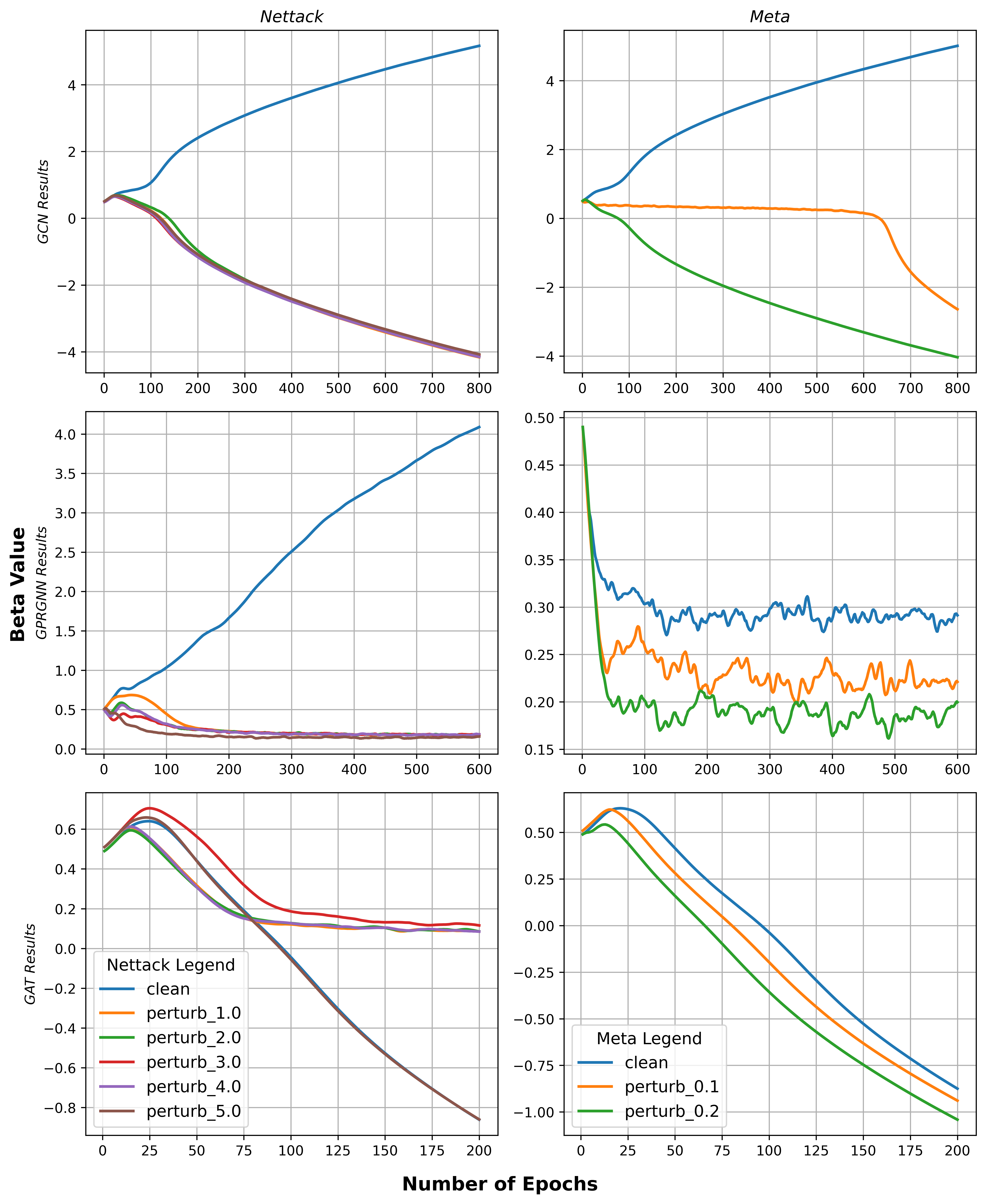
Furthermore, the learnable weight of the averaging variable, , is tracked during training, as depicted by Fig. 1. The intuition that can serve as an effective parameter for assessing attack severity is supported by the observation that, in most cases, values are distinguishable for clean graphs. This trajectory also shows that the severity levels can be distinguishable either, considering how varied between different perturbation rates, i.e. for all models under Metattack in Fig. 1. The early estimation of allows practitioners to identify the presence and severity of adversarial attacks during the initial stages of the training process, enabling proactive measures to improve model robustness before training is completed.
Fig. 1 also shows a result that contradicts the intuition behind learning the values, when GAT is used as the backbone model under Nettack attack on the Pubmed dataset. This is particularly interesting because, despite -GNN showing significant performance improvement over vanilla GAT (84.30% vs 71.67% accuracy for 5-edge perturbations), the values do not show a clear separation between clean and perturbed cases. This suggests that while the ensemble model effectively enhances model robustness, the mechanism of improvement might be different from other backbone architectures. Rather than clearly down-weighting the GAT component under attack, the model might be finding a more complex integration strategy between GAT and MLP that leverages GAT’s attention mechanism in conjunction with MLP’s feature processing, even under perturbation.
In addition to the experiments that compare the proposed method against the vanilla backbone models, we compare -GNN against other defense methods. Table 4 and 5 present the benchmark results, where GPRGNN is used as the backbone for the proposed method due to its excellent performance on heterophilic datasets. For simplicity, we only present results for perturbed graphs with a perturbation budget of 5 edges per target node for Nettack, and a perturbation ratio of 20% for Metattack in Table 4 and 5.
4.3. Complexity Analysis
Computational efficiency is crucial to real-world applicability of defense methods. Herein, we analyze the time and space complexity of -GNN and other defense models. Let be the number of iterations in Pro-GNN’s optimization process, be the number of nodes, be the number of edges, be the number of graph convolutional layers, be the feature dimension, be the hidden layer dimension, and be the number of top singular vectors retained in GCN-SVD.
-
•
Pro-GNN introduces significant computational overhead through iterative structure learning, rendering it impractical for large-scale graphs. With our experimental setup, Pro-GNN takes almost 2 days to train on Squirrel graph to produce the reported results. Its time complexity is , and its space complexity is .
-
•
GCN-Jaccard is comparably better than other benchmarks in terms of its time complexity. However, the quadratic edge similarity computation limits its scalability for dense graphs. Furthermore, its performance on heterophilic graphs is even lower than GCN-Vanilla, according to Table 4 and 5. Its time complexity and space complexity can be expressed as and , respectively.
-
•
RGCN introduces additional computational complexity through Gaussian-based graph learning. Along with Pro-GNN and GCN-SVD, RGCN cannot scale to larger graphs, as evidenced by our evaluations on the Pubmed dataset, where it results in an out-of-memory error. The time complexity of RGCN is , whereas its space complexity is
-
•
GCN-SVD introduces cubic complexity due to applying singular value decomposition, severely restricting scalability. Computing the full matrix eigendecomposition requires computation complexity and results in a high time complexity for GCN-SVD. Its space complexity is , where needs to increase as the graph size grows.
-
•
-GNN method achieves linear scalability by avoiding expensive graph structure preprocessing. The time complexity of the proposed method is , while its space complexity is .
We observe that cubic complexity models (Pro-GNN, GCN-SVD) become impractical for graphs with nodes. Similarly, quadratic models (RGCN) face significant performance degradation. In contrast, -GNN, as a linear complexity model, maintains consistent performance across varying graph scales.
5. Conclusion
In this work, we introduced -GNN, a novel approach to enhance GNN robustness by dynamically weighting the contribution of a base GNN model and an MLP through a learned parameter. This ensemble method not only improves resilience against adversarial attacks but also provides an interpretable measure of data perturbation severity. Our experiments demonstrate the effectiveness of -GNN in improving node classification accuracy under attack, particularly in preserving performance on unperturbed data structures. The linear computational complexity of -GNN offers a significant advantage for scalability in large-scale applications.
While -GNN demonstrates promising results, it is not without limitations. Specifically, while the learned values often provide a clear distinction between clean and perturbed data instances, this separation is not always guaranteed. In some cases, the tracks of values for clean and perturbed data can intertwine, making it challenging to definitively distinguish between them. Future work will address this limitation by investigating methods to improve the separation of value tracks, potentially through incorporating additional features or constraints during the learning process. This could involve exploring more sophisticated regularization techniques or examining the influence of different base GNN architectures on the behavior of .
Acknowledgements.
This paper was supported by the Swarmchestrate project of the European Union’s Horizon 2023 Research and Innovation programme under grant agreement no. 101135012.References
- (1)
- Andrychowicz et al. (2016) M. Andrychowicz, M. Denil, S. G. Colmenarejo, M. W. Hoffman, D. Pfau, T. Schaul, et al. 2016. Learning to learn by gradient descent by gradient descent. In Proceedings of the 30th International Conference on Neural Information Processing Systems (Barcelona, Spain) (NIPS’16). Curran Associates Inc., Red Hook, NY, USA, 3988–3996.
- Bilot et al. (2023) Tristan Bilot, Nour El Madhoun, Khaldoun Al Agha, and Anis Zouaoui. 2023. Graph Neural Networks for Intrusion Detection: A Survey. IEEE Access 11 (2023), 49114–49139. doi:10.1109/ACCESS.2023.3275789
- Chien et al. (2021) E. Chien, J. Peng, P. Li, and O. Milenkovic. 2021. Adaptive Universal Generalized PageRank Graph Neural Network. In International Conference on Learning Representations. https://openreview.net/forum?id=n6jl7fLxrP
- Dai et al. (2024) Enyan Dai, Tianxiang Zhao, Huaisheng Zhu, Junjie Xu, Zhimeng Guo, Hui Liu, Jiliang Tang, and Suhang Wang. 2024. A comprehensive survey on trustworthy graph neural networks: Privacy, robustness, fairness, and explainability. Machine Intelligence Research (2024), 1–51.
- Deng et al. (2022) C. Deng, X. Li, Z. Feng, and Z. Zhang. 2022. GARNET: Reduced-Rank Topology Learning for Robust and Scalable Graph Neural Networks. In Proceedings of the First Learning on Graphs Conference, Vol. 198. 3:1–3:23. https://proceedings.mlr.press/v198/deng22a.html
- Di Massa et al. (2006) V. Di Massa, G. Monfardini, L. Sarti, F. Scarselli, M. Maggini, and M. Gori. 2006. A Comparison between Recursive Neural Networks and Graph Neural Networks. In The 2006 IEEE International Joint Conference on Neural Network Proceedings. Vancouver, BC, Canada, 778–785. doi:10.1109/IJCNN.2006.246763
- Entezari et al. (2020a) N. Entezari, S. A. Al-Sayouri, A. Darvishzadeh, and E. E. Papalexakis. 2020a. All You Need Is Low (Rank): Defending Against Adversarial Attacks on Graphs. In Proceedings of the 13th International Conference on Web Search and Data Mining (Houston, TX, USA) (WSDM ’20). Association for Computing Machinery, New York, NY, USA, 169–177. doi:10.1145/3336191.3371789
- Entezari et al. (2020b) N. Entezari, S. A. Al-Sayouri, A. Darvishzadeh, and E. E. Papalexakis. 2020b. All You Need Is Low (Rank): Defending Against Adversarial Attacks on Graphs. In Proceedings of the 13th International Conference on Web Search and Data Mining (Houston, TX, USA) (WSDM ’20). Association for Computing Machinery, New York, NY, USA, 169–177. doi:10.1145/3336191.3371789
- Fan et al. (2019) W. Fan, Y. Ma, Q. Li, Y. He, E. Zhao, J. Tang, and D. Yin. 2019. Graph Neural Networks for Social Recommendation. In The World Wide Web Conference (San Francisco, CA, USA) (WWW ’19). Association for Computing Machinery, New York, NY, USA, 417–426. doi:10.1145/3308558.3313488
- Geisler et al. (2021) S. Geisler, T. Schmidt, H. Şirin, D. Zügner, A. Bojchevski, and S. Günnemann. 2021. Robustness of Graph Neural Networks at Scale. In Neural Information Processing Systems, NeurIPS.
- Jin et al. (2020) Wei Jin, Yao Ma, Xiaorui Liu, Xianfeng Tang, Suhang Wang, and Jiliang Tang. 2020. Graph Structure Learning for Robust Graph Neural Networks. In 26th ACM SIGKDD International Conference on Knowledge Discovery and Data Mining, KDD 2020. Association for Computing Machinery, 66–74.
- Kipf and Welling (2016) T. N. Kipf and M. Welling. 2016. Semi-Supervised Classification with Graph Convolutional Networks. CoRR abs/1609.02907 (2016). arXiv:1609.02907 http://arxiv.org/abs/1609.02907
- Li et al. (2020) Y. Li, W. Jin, H. Xu, and J. Tang. 2020. DeepRobust: A PyTorch Library for Adversarial Attacks and Defenses. CoRR abs/2005.06149 (2020). arXiv:2005.06149 https://arxiv.org/abs/2005.06149
- Liu and Huang (2023) Chien-Liang Liu and Tzu-Hsuan Huang. 2023. Dynamic Job-Shop Scheduling Problems Using Graph Neural Network and Deep Reinforcement Learning. IEEE Transactions on Systems, Man, and Cybernetics: Systems 53, 11 (2023), 6836–6848. doi:10.1109/TSMC.2023.3287655
- Liu et al. (2024) S. Liu, X. Zhou, J. Yu, Y. Wang, T. Xu, and H. Wang. 2024. Graph Attention Network-Based Model for Multiple Fault Detection and Identification of Sensors in Nuclear Power Plant. Nuclear Engineering and Design 419 (2024), 112949. doi:10.1016/j.nucengdes.2024.112949
- McCallum et al. (2000) A. K. McCallum, K. Nigam, J. Rennie, and K. Seymore. 2000. Automating the construction of internet portals with machine learning. Information Retrieval 3 (2000), 127–163.
- Mirhoseini et al. (2021) A. Mirhoseini, A. Goldie, M. Yazgan, J. W. Jiang, E. Songhori, S. Wang, Y.-J. Lee, E. Johnson, O. Pathak, A. Nazi, et al. 2021. A graph placement methodology for fast chip design. Nature 594, 7862 (2021), 207–212.
- Rahmani et al. (2023) S. Rahmani, A. Baghbani, N. Bouguila, and Z. Patterson. 2023. Graph Neural Networks for Intelligent Transportation Systems: A Survey. IEEE Transactions on Intelligent Transportation Systems 24, 8 (2023), 8846–8885. doi:10.1109/TITS.2023.3257759
- Rozemberczki et al. (2021) B. Rozemberczki, C. Allen, and R. Sarkar. 2021. Multi-Scale Attributed Node Embedding. Journal of Complex Networks 9, 2 (April 2021). doi:10.1093/comnet/cnab014
- Sen et al. (2008) P. Sen, G. Namata, M. Bilgic, L. Getoor, B. Galligher, and T. Eliassi-Rad. 2008. Collective classification in network data. AI magazine 29, 3 (2008), 93–93.
- Veličković et al. (2018) P. Veličković, G. Cucurull, A. Casanova, A. Romero, P. Liò, and Y. Bengio. 2018. Graph Attention Networks. In International Conference on Learning Representations. https://openreview.net/forum?id=rJXMpikCZ
- Wu et al. (2019) Huijun Wu, Chen Wang, Yuriy Tyshetskiy, Andrew Docherty, Kai Lu, and Liming Zhu. 2019. Adversarial Examples for Graph Data: Deep Insights into Attack and Defense. In Proceedings of the Twenty-Eighth International Joint Conference on Artificial Intelligence, IJCAI-19. International Joint Conferences on Artificial Intelligence Organization, 4816–4823. doi:10.24963/ijcai.2019/669
- Wu et al. (2022) X. Wu, H. Wu, X. Zhou, X. Zhao, and K. Lu. 2022. Towards defense against adversarial attacks on graph neural networks via calibrated co-training. Journal of Computer Science and Technology 37, 5 (2022), 1161–1175.
- Yang et al. (2022) Jianbang Yang, Dahai Tang, Xiaoniu Song, Lei Wang, Qiang Yin, Rong Chen, Wenyuan Yu, and Jingren Zhou. 2022. GNNLab: a factored system for sample-based GNN training over GPUs (EuroSys ’22). Association for Computing Machinery, New York, NY, USA, 417–434. doi:10.1145/3492321.3519557
- Zhang and Zitnik (2020) X. Zhang and M. Zitnik. 2020. GNNGuard: Defending Graph Neural Networks against Adversarial Attacks. In NeurIPS.
- Zhu et al. (2019) D. Zhu, Z. Zhang, P. Cui, and W. Zhu. 2019. Robust Graph Convolutional Networks Against Adversarial Attacks. In Proceedings of the 25th ACM SIGKDD International Conference on Knowledge Discovery & Data Mining (Anchorage, AK, USA) (KDD ’19). Association for Computing Machinery, New York, NY, USA, 1399–1407. doi:10.1145/3292500.3330851
- Zhu et al. (2022) J. Zhu, J. Jin, D. Loveland, M. T. Schaub, and D. Koutra. 2022. How does Heterophily Impact the Robustness of Graph Neural Networks? Theoretical Connections and Practical Implications. In Proceedings of the 28th ACM SIGKDD Conference on Knowledge Discovery and Data Mining (Washington DC, USA) (KDD ’22). Association for Computing Machinery, New York, NY, USA, 2637–2647. doi:10.1145/3534678.3539418
- Zola et al. (2022) F. Zola, L. Segurola-Gil, J. L. Bruse, M. Galar, and R. Orduna-Urrutia. 2022. Network Traffic Analysis through Node Behaviour Classification: A Graph-Based Approach with Temporal Dissection and Data-Level Preprocessing. Computers & Security 115 (2022), 102632. doi:10.1016/j.cose.2022.102632
- Zügner et al. (2018) D. Zügner, A. Akbarnejad, and S. Günnemann. 2018. Adversarial Attacks on Neural Networks for Graph Data. Proceedings of the 24th ACM SIGKDD International Conference on Knowledge Discovery & Data Mining (2018). https://api.semanticscholar.org/CorpusID:29169801
- Zügner and Günnemann (2019) D. Zügner and S. Günnemann. 2019. Adversarial Attacks on Graph Neural Networks via Meta Learning. CoRR abs/1902.08412 (2019). arXiv:1902.08412 http://arxiv.org/abs/1902.08412