Localizing entropy production along non-equilibrium trajectories

Abstract

An important open problem in nonequilibrium thermodynamics is the quantification and spatiotemporal localization of entropy production in complex nanoscale processes from experimental data. Here we address this issue through a data-driven approach that combines the recently developed short-time thermodynamic uncertainty relation based inference scheme with machine learning techniques. Our approach leverages the flexible function representation provided by deep neural networks to achieve accurate reconstruction of high-dimensional, potentially time-dependent dissipative force fields as well as the localization of entropy production in both space and time along nonequilibrium trajectories. We demonstrate the versatility of the framework through applications to diverse systems of fundamental interest and experimental significance, where it successfully addresses distinct challenges in localizing entropy production.

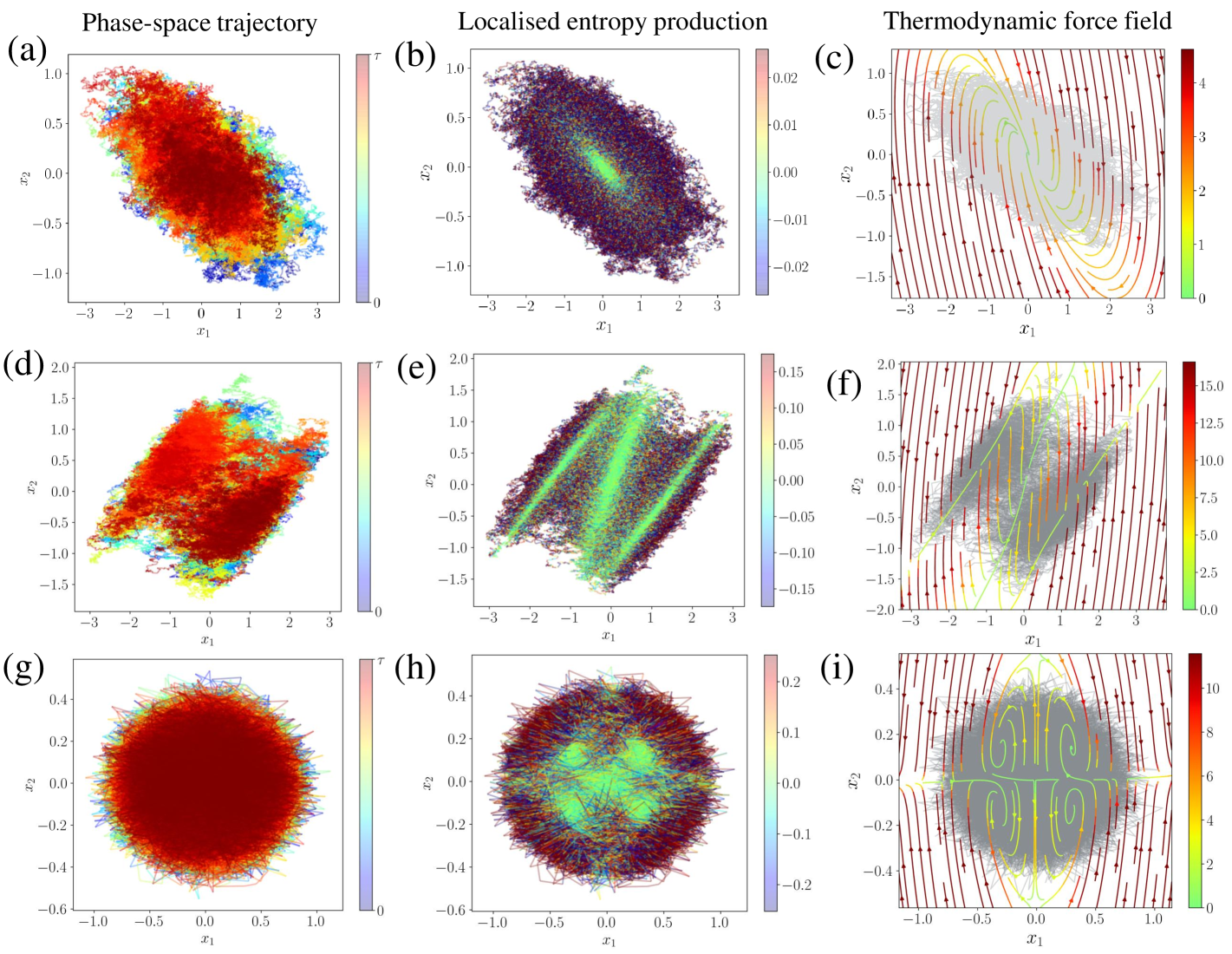
Figure 1: Brownian gyrator model: (a) 2D-dimensional trajectories of a Brownian gyrator system with harmonic confining potential. [Parameters: $k_{1}=1$, $k_{2}=2$, $\gamma=1$, $\theta=\pi/4$, $D_{1}=1$, $D_{2}=0.1$]. (b) local entropy production rate and (c) thermodynamic force field for the system with harmonic confinement - estimated using the neural network representation. (d) 2D-dimensional trajectories of a Brownian gyrator system with a bi-stable confining potential. [Parameters: $k=1$, $b=1$, $\gamma=1$, $\theta=\pi/4$, $D_{1}=1$, $D_{2}=0.1$] (e) local entropy production rate and (f) thermodynamic force field estimated using the neural network representation. (g) 2D-dimensional trajectories of a Brownian gyrator system with a quartic confining potential. [Parameters: $k_{1}=k_{2}=10$, $\gamma=1$, $\theta=\pi/4$, $D_{1}=10$, $D_{2}=1$] (h) local entropy production rate and (i) thermodynamic force field estimated using the neural network representation. The colours corresponding to the local entropy production rate (in units of $k_{B}/s$) of the gyrators are thresholded to visualise the anisotropy present in the local dissipation map and do not indicate the actual values. The true magnitude of the thermodynamic force field for the gyrators are normalised by the corresponding median values. The numerical trajectories are usually generated for $2000s$ with a sampling rate of $1\ kHz$ - from which trajectory traces of $500s$ are shown in the plots.

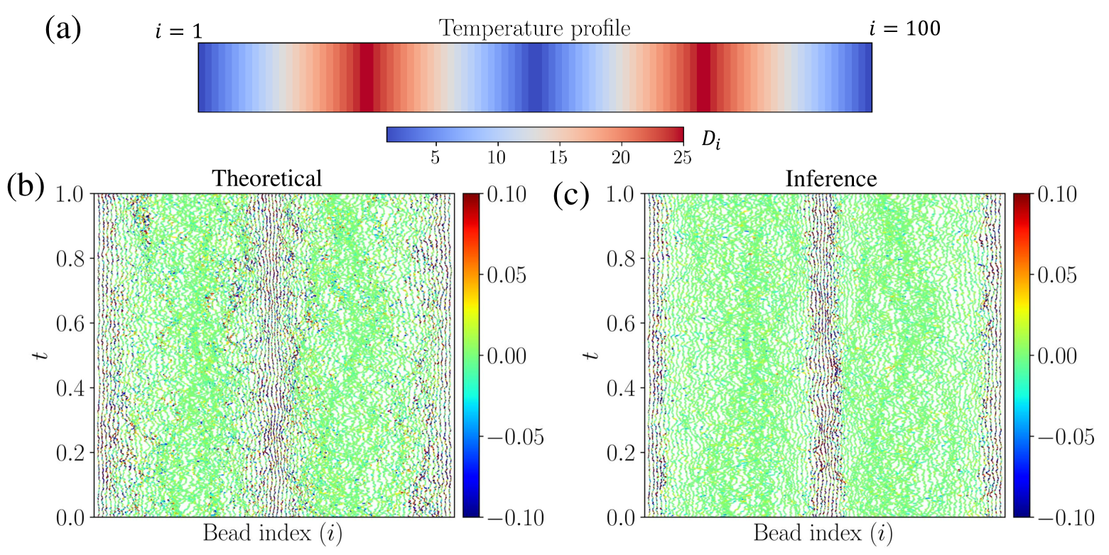
Figure 2: (a) Temperature profile of the $N$-dimensional gyrator setup. (b) Analytically estimated local entropy production rate (in units of $k_{B}/s$) of the system. (c) Local entropy production rate (in units of $k_{B}/s$) inferred from the numerical trajectories using a neural network representation. The colors do not indicate the true values of the fluctuating entropy current, but they are thresholded for better visualisation.

I Introduction

Processes that operate far from thermodynamic equilibrium are ubiquitous in nature [1]. They are characterized by non-vanishing phase space fluxes and the continuous dissipation of energy into their surroundings [2, 3]. Extracting the underlying dissipative force fields and the associated energetic costs from experimentally tractable observations, such as single-molecule trajectories, fluorescence imaging, or spectroscopic data is a challenging task and a vastly developing field of research [4, 5, 6, 7, 8, 9, 10, 11, 12, 13, 14, 15]. Recent advances in this field, primarily driven by the developments in stochastic thermodynamics [16, 17, 18], combine far-from-equilibrium statistical physics with nanoscale experiments/simulations and data-driven approaches [19, 20, 21, 22, 11]. These methods have, for example, successfully quantified entropy production in cellular processes where dissipation rates could be orders of magnitude below the detection limits of conventional calorimetry [10, 12, 23, 24, 13].

One of the main contributions of this field is the rigorous formulation of entropy production along individual, fluctuating realizations of nanoscale nonequilibrium processes [25, 17]. The rate of entropy production ($\sigma$) in such a process then quantifies, simultaneously, the breaking of time-reversal symmetry of the process, as well as the continuos dissipation of energy to the surroundings [26]. Furthermore, a non-vanishing conjugate force field, referred to as the thermodynamic force field ${\bm{F}}({\bm{x}},t)$, can always be associated with nonequilibrium processes. When contracted with the infinitesimal increment of the phase space trajectory $d{\bm{x}}_{t}$, this force field yields the local entropy production along the trajectory [19]. The thermodynamic force field vanishes everywhere in space and time when the system is at equilibrium; thus, it governs the local dissipative dynamics, providing a direct link between microscopic irreversibility and energy dissipation.

Despite their fundamental importance, directly measuring the entropy production or dissipative force field from experimental data remains a significant challenge. Conventional approaches rely on the knowledge of the underlying dynamical equations, such as Fokker-Planck and Master equations, and their solutions, which are often unknown in realistic settings. In a number of such cases, in principle, a global estimate of the entropy production rate of a process can be directly estimated from experimental data, particularly for systems with Markovian dynamics, using a variety of methods. These include the application of the Harada-Sasa equality [6], which involves perturbing systems from the non-equilibrium steady state and analyzing their response; methods that depend on the estimation of the average steady-state currents and the steady-state probability distribution [5]; and time-irreversibility measures, which quantify the breaking of time-reversal symmetry in the dynamics [27, 28, 26, 29, 30, 31]. Path probability estimators, which compute the relative probabilities for forward and time-reversed trajectories directly from data, have also been developed [4, 32, 33]. For overdamped diffusive processes, another approach involves inferring the drift and diffusion terms from experimental data [7, 8], from which $\sigma$ can subsequently be deduced. A more recent method, called the variance sum rule (VSR), derives a formula for the entropy production rate $\sigma$ by incorporating the second derivative of the position correlation function and the covariances of microscopic forces [13]. While its direct application was initially limited by experimental challenges in measuring mobility and forces, a recently proposed modification to VSR has overcome this limitation [34].

In addition to these approaches, a number of variational optimization schemes have been developed to quantify the entropy production rate. A notable method is based on the thermodynamic uncertainty relation (TUR) [35, 36, 37, 38, 39, 40, 21, 41, 42, 19], which translates the task of identifying entropy production into an optimization problem over the space of a single projected fluctuating current in the system. Unlike trajectory-based methods that require estimating probability distributions over the phase space, these inference schemes typically rely only on the means and variances of measured currents, making them more effective for higher-dimensional systems [19]. For overdamped diffusive processes, it has since been shown that such optimization problems yield the exact value of the entropy production rate, as well as the exact thermodynamic force field, provided that short-time currents are used [38, 40, 39] – hereafter we refer to this method as the the short-time inference scheme. Notably, this method works in both stationary regimes [21] and in time-dependently driven cases [20]. A similar variational approach using neural networks has also been proposed [22], where the estimator includes an exponential average over current fluctuations. This method has the additional advantage of being applicable to both overdamped diffusive processes and Markov jump processes while also saturating for both [39].

The aforementioned methods have primarily focused on obtaining global estimates of the entropy production rate. However, there are a few notable exceptions [19, 22, 14, 15, 11]. In Ref. [19], the authors developed a brute-force statistical binning approach to estimate the thermodynamic force field. However, this method scales poorly to higher dimensional systems. The method proposed in Ref. [22] directly learns entropy production along trajectories, though it does not explicitly reveal the structure of the underlying dissipative force field. In Ref. [14, 15], the authors introduced a notion of ‘Markovian events’ which help define fluctuating entropy production for coarse-grained processes in a thermodynamically consistent manner. Most recently, Ref. [11] demonstrated how to learn part of the dissipative force field from data while requiring that the remaining components are known a priori. However, they have provided nice demonstrations of spatiotemporally localized dissipation in the stationary states of high-dimensional interacting active particle systems.

Here, we show that combining the short-time inference scheme with well-established machine learning techniques offers a model-independent route to localizing entropy production even along time-dependent nonequilibrium trajectories. Using flexible neural network architectures and building on the short-time TUR based algorithms previously proposed in Refs. [9, 40, 39, 20, 21], we demonstrate the ability to accurately reconstruct complex, high-dimensional thermodynamic force fields and resolve local contributions to entropy production—localized in both space and time—directly from observed data. We illustrate the versatility and robustness of our framework through applications to diverse experimental systems, each presenting unique challenges for localizing entropy production.

The paper is organized as follows. In Section II, we provide an overview of the TUR-based short-time inference scheme and present a machine learning algorithm to perform the inference. Section III demonstrates applications of the method to experimentally relevant systems that present distinct challenges for conventional entropy production rate estimation. Finally, Section IV concludes with an outlook.

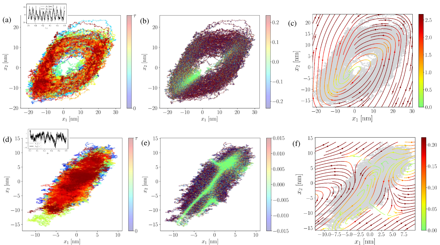
Figure 3: Hair-cell bundle oscillation:(a) Representation of numerical 2D-trajectories in the $(x_{1},x_{2})$ phase space corresponding to $5s$ simulation sampled at $100\ kHz$. The inset plot indicates the oscillatory nature of dynamics for $F_{max}=57.14\ pN$ and $S=0.94$. (b) The local entropy production rate (in units of $k_{B}/s$) is computed using the neural network representation. It captures the active state of dynamics. The colours are for comparative visualisation and do not represent the true value. (c) Thermodynamic force field of the oscillatory state of the dynamics. Here, the magnitude of the force field is normalised by the median value. (d) Representation of numerical 2D-trajectories in the $(x_{1},x_{2})$ phase space corresponding to $5s$ simulation sampled at $100\ kHz$. The inset plot indicates the quiescent (non-oscillatory) state of dynamics for $F_{max}=40\ pN$ and $S=0.94$. (e) Entropy production rate (in units of $k_{B}/s$) is locally computed along such trajectories. The colours are for comparative visualisation and do not represent the true value. (f) Thermodynamic force field of the oscillatory state of the dynamics. Here, the magnitude of the force field is normalised by the median value. The other system parameters remain the same as mentioned in Fig.(4) of Ref. [12]: $\gamma_{1}=2.8\ \mu N\ s/m$, $\gamma_{2}=10\ \mu N\ s/m$, $k_{\text{gs}}=0.75\ pN/nm$, $k_{\text{sp}}=0.6\ pN/nm$, $D=61\ nm$, $N=50$, $\Delta G=10k_{B}T$, $k_{B}T=4.143\ pNnm$ and $T_{eff}=1.5T$.

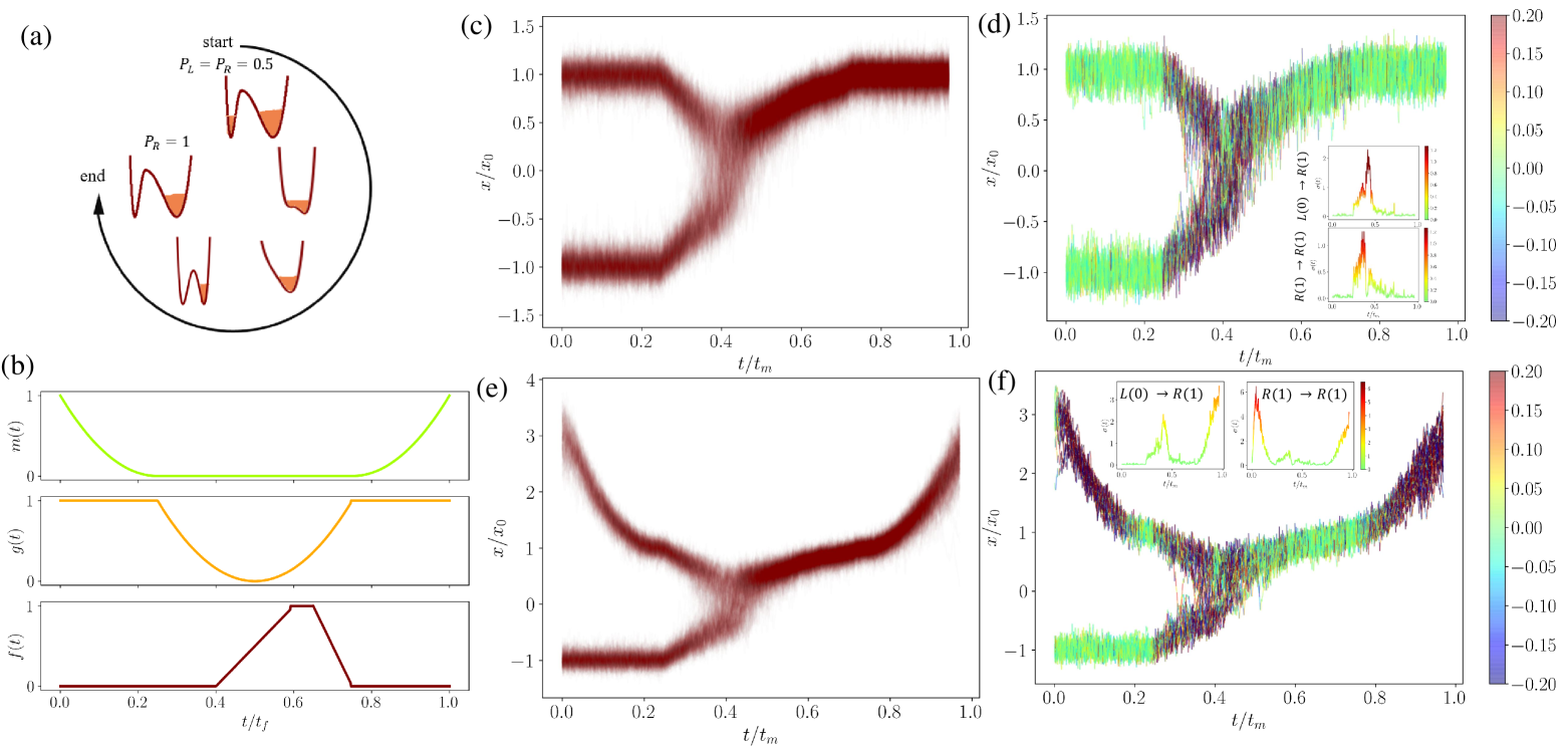
Figure 4: Bit-erasure protocol: (a) Schematic of a bit-erasure protocol. The probability of finding the particle in one of the wells is equal ($P_{L}=P_{R}=0.5$) at the onset and at the end of the protocol, the particle ends up in the right well with $P_{R}=1$. (b) Plot of the time-dependent control functions: $m(t)$, $g(t)$ and $f(t)$. We used the functional form of these functions as provided in the supplementary of Ref. [43]. (c) Representative trajectories undergoing erasing protocol in a symmetric potential ($\eta=1$). (d) Trajectories with the localised entropy production rate (in units of $k_{B}/s$) of the particle during the erasing process with a symmetric potential. (e) Representative trajectories undergoing erasing protocol in an asymmetric potential ($\eta=1$) (f) Trajectories with the localised entropy production rate (in units of $k_{B}/s$) of the particle during the erasing process with an asymmetric potential ($\eta=3$). In both cases, the local entropy production rate is estimated using the learning technique. The colour bar does not indicate the true value but is thresholded for better visualisation. The insets of both (d) and (f) are the plots of the mean entropy production rate over the cycle time and the corresponding colorbar represents the actual value of the average entropy production rate. Those curves are smoothened with moving averages over 5 points. [Parameters: $E_{b}=13k_{B}T$, $k_{B}T=4.14\times 10^{-3}pN\mu m$, $A=0.3$, $x_{m}=0.77\mu m$, $D=0.23\mu m^{2}/s$, $t_{m}\equiv(2x_{0})^{2}/D=10s$.]

II Methods

The methods discussed in this work are applicable to experimental data from overdamped diffusive processes but do not require the knowledge of their underlying equations. To establish notations and definitions, we introduce a generic overdamped Langevin model in a $d$ -dimensional space, described by:

$$\dot{{\bm{x}}}(t)={\bm{A}}({\bm{x}}(t),t)+{\bm{B}}({\bm{x}}(t),t)\cdot{\bm{\xi}}(t),$$ (1)

where ${\bm{A}}({\bm{x}},t)$ is the drift vector, and ${\bm{B}}({\bm{x}},t)$ is a $d\times d$ matrix, and ${\bm{\xi}}(t)$ represents a Gaussian white noise satisfying $\langle\xi_{i}(t)\xi_{j}(t^{\prime})\rangle=\delta_{ij}\delta(t-t^{\prime})$. Both ${\bm{A}}({\bm{x}},t)$ and ${\bm{D}}({\bm{x}},t)$ could be non-linear functions in ${\bm{x}}$ and $t$.

The Fokker-Planck equation that describes the time evolution of the probability density function $p({\bm{x}},t)$ is given by,

$$\partial_{t}p({\bm{x}},t) =-{\bm{\nabla}}\;{\bm{j}}({\bm{x}},t),$$ (2)

$$j_{i}({\bm{x}},t) =A_{i}({\bm{x}},t)p({\bm{x}},t)-\sum_{j}\nabla_{j}\left[D_{ij}({\bm{x}},t)p({\bm{x}},t)\right],$$ (3)

where $\bm{D}$ is the diffusion matrix defined as

$${\bm{D}}({\bm{x}},t)=\frac{1}{2}{\bm{B}}({\bm{x}},t){\bm{B}}({\bm{x}},t)^{T}$$ (4)

and ${\bm{j}}({\bm{x}},t)$ is the probability current.

A nonvanishing probability current — ${\bm{j}}({\bm{x}},t)\neq 0$ is then a characteristic property of a process that is out of equilibrium. The extent of the non-equilibrium character can then be quantified using the average rate of the entropy production at a given instant $\sigma(t)$, defined as [44]

$$\sigma(t)=\int{\rm d}{\bm{x}}\;{\bm{F}}({\bm{x}},t)\;{\bm{j}}({\bm{x}},t),$$ (5)

where ${\bm{F}}({\bm{x}},t)$ is the conjugate thermodynamic force field or dissipative force field defined as

$${\bm{F}}({\bm{x}},t) =\frac{{\bm{j}}^{T}({\bm{x}},t){\bm{D}}({\bm{x}},t)^{-1}}{p({\bm{x}},t)}.$$ (6)

Here we have set Boltzmann’s constant $k_{B}=1$. Further, when contracted with the infinitesimal increment of the phase space trajectory $d{\bm{x}}_{t}$, this force field yields the local entropy production along the trajectory as

$${\rm d}S={\bm{F}}\left({\bm{x}}(t),t\right)\circ{\rm d}{\bm{x}}(t),$$ (7)

where $\circ$ denotes the Stratonovich product.

Indeed, if the explicit form of the overdamped equation in Eq. (1), as well as the Fokker-Planck equation in Eq. (2) and it’s time dependent solution are known, one can straight forwardly determine the functional form of the thermodynamic force field in Eq. (6), and use that to evaluate entropy production along any individual realization of the process. However, this is only possible in a limited number of analytically tractable cases. In the following we discuss a variational representation that can estimate $\sigma(t)$, ${\bm{F}}({\bm{x}},t)$ and $S[{\bm{x}}(\cdot),t]$ from overdamped non-equilibrium trajectories, without requiring the prior knowledge of the dynamical equations or their solution.

II.1 Inferring local entropy production using the short-time TUR

Our approach is based on the thermodynamic uncertainty relation (TUR), which provided a universal constraint on non-equilibrium current fluctuations in terms of the entropy production rate [35]. In the original form, TUR provides a lower bound for the entropy production rate in terms of the first two cumulants of non-equilibrium current fluctuations in a steady state as,

$$\sigma\geq\frac{2\left<J_{\bm{d}}\right>^{2}}{\tau{\rm Var}(J_{\bm{d}})},$$ (8)

where $J_{\bm{d}}$ is a generalized current of length $\tau$ given by $J_{\bm{d}}:=\int_{{\bm{x}}(0)}^{{\bm{x}}(\tau)}{\bm{d}}({\bm{x}}(t))\circ{\rm d}{\bm{x}}(t)$ defined with some coefficient field ${\bm{d}}({\bm{x}})$. The originally known limit in which the lower bound saturates is the equilibrium limit where $\sigma\rightarrow 0$. It was then shown that, for overdamped Langevin dynamics, TUR also saturates in the $\tau\rightarrow 0$ limit of current fluctuations[38, 40, 39]. Crucially, the proof in Ref. [40] is also valid for non-stationary dynamics.
This gives a variational representation of the entropy production rate, as

$$\sigma_{\rm TUR}(t):=\frac{1}{{\rm d}t}\max_{{\bm{d}}}\frac{2\left<J_{\bm{d}}\right>^{2}}{{\rm Var}(J_{\bm{d}})},$$ (9)

where $J_{\bm{d}}$ is the (single-step) generalized current given by $J_{\bm{d}}:={\bm{d}}({\bm{x}}(t))\circ{\rm d}{\bm{x}}(t)$. The expectation and the variance are taken with respect to the joint probability density $p({\bm{x}}(t),{\bm{x}}(t+{\rm d}t))$. In the ideal short-time limit ${\rm d}t\to 0$, the estimator gives the exact value, i.e., $\sigma_{\rm TUR}(t)=\sigma(t)$ holds. Further, the optimal coeffficient field is known to be proportional to the thermodynamic force field as ${\bm{d}}^{*}({\bm{x}})=c{\bm{F}}({\bm{x}},t)$, where the constant factor $c$ can be fixed using the relation $2\left<J_{\bm{d}}\right>/{\rm Var}(J_{\bm{d}})=1/c$.

II.2 Machine learning the dissipative force field and entropy production

The variational representation of the $\sigma(t)$ given in Eq. (9) takes a form that is well-established in control theory. A common strategy in such settings is to approximate the optimal solution, the thermodynamic force field, using a parameterized function ${\bm{d}}({\bm{x}},{\bm{\theta}})$, where ${\bm{\theta}}$ represents a set of tunable parameters. However, the complexity of high-dimensional, many-body interactions poses significant challenges for traditional optimization methods. To overcome these difficulties, we leverage gradient-based techniques enhanced by deep neural networks, which excel at approximating complex, high-dimensional functions [45, 46, 47, 48, 49, 50]. This combination enables efficient exploration of the parameter space, even in scenarios where analytical solutions are intractable. The detailed steps of our approach are outlined in Algorithm 1, as well as in the accompanying Python implementation [51]. See also Refs. [40, 20, 21] for earlier implementations of this algorithm.

Building on recent advances in the deep Ritz method [52, 53], we model the dissipative force field using a parameterized representation:

$${\bm{F}}({\bm{x}},t)={\bm{d}}({\bm{x}},t;\theta).$$ (10)

Initially, we restrict our analysis to stationary non-equilibrium processes, where we can remove the explicit time dependence in Eq. (10). Our approach builds on a neural network architecture previously used in Ref. [54], where the authors combined optimal control theory techniques with the flexible function representation provided by deep neural networks to efficiently sample rare events in interacting many-body systems. Inspired by this study, we model the function $\bm{d}(\bm{x})$ by a multi-layer neural network structure with hidden layers $\{L_{i}\}$. Each layer consists of two linear transformations, two nonlinear activation functions, and a residual connection, defined as:

$$L_{i}({\bm{x}})=\Phi\left[W_{i,2}\cdot\phi(W_{i,1}{\bm{x}}+b_{i,1})+b_{i,2}\right]+{\bm{x}},$$ (11)

where $W_{i,j}\in\mathbb{R}^{h\times h}$ and $b_{i,j}\in\mathbb{R}^{h}$ are the trainable parameters of the $i$-th layer, $h$ is the hidden layer dimension, and $\Phi$ denotes the activation function. The residual connection, formulated as $L_{i}({\bm{x}})=f({\bm{x}})+{\bm{x}}$, enhances training stability and alleviates issues related to vanishing gradients. We utilize the bounded $\tanh(\cdot)$ activation function across the network, although alternative nonlinearities could also be employed. The complete network is constructed as a composition of these layers:

$${\bm{z}}({\bm{x}},{\bm{\theta}})=L_{n}\circ\dots\circ L_{1}({\bm{x}}).$$ (12)

The thermodynamic force field ${\bm{d}}({\bm{x}},{\bm{\theta}})\in\mathbb{R}^{d}$ is then obtained as a linear transformation of the network’s output ${\bm{z}}({\bm{x}},{\bm{\theta}})$.

Note that, this framework redefines the task of measuring entropy production in nonequilibrium systems as a machine learning challenge centered on approximating the associated dissipative force field. This strategy eliminates the reliance on explicit dynamical descriptions of the process, and offers a scalable solution for analyzing entropy production in systems with intricate interactions. Once trained, the machine-learned force field can be used to visualize entropy production along non-equilibrium trajectories, enabling the localization of entropy production in both space ${\bm{x}}$ and time $t$. We note that this idea aligns closely with the approach of Ref. [11]. However, their method relies on prior knowledge of the underlying dynamical equations to construct part of the dissipative force field, whereas in our framework, the quantity is learned entirely from data.

In the following, we demonstrate that the architecture we use is versatile and applicable to a wide range of processes, each presenting unique challenges in localizing entropy production.

III Applications

We test our algorithm in this section on several models, which have been studied before in the stochastic thermodynamics context, and which illustrate different challenges in estimating entropy production.

III.1 Stationary non-equilibrium systems: Brownian Gyrators

Brownian gyrator is a simplistic model of an autonomous heat engine [55, 56]. In it’s most basic implementation, a mesoscopic particle is confined in a two-dimensional conservative potential in the presence of two heat baths at different temperatures. The dynamics of the system can be expressed as a $2D$ overdamped Langevin equation as,

$$\gamma\dot{x}_{i}(t)=-\ \partial_{x_{i}}U(x_{i},x_{j})+\sqrt{2D_{i}\gamma^{2}}\xi_{i}(t),$$ (13)

with $\langle\xi_{i}(t)\rangle=0$, $\langle\xi_{i}(t)\xi_{j}(t^{\prime})\rangle=\delta_{ij}\delta(t-t^{\prime})$. Here, the viscous drag of the medium is denoted as $\gamma$, and $D_{i}=k_{B}T_{i}/\gamma$ denotes the diffusion constants along two directions, which are proportional to the temperatures ($T_{i}$) of the corresponding baths. In the absence of any coupling through the potential between the degrees of freedom of the system, each degree reaches an equilibrium steady state characterised by the temperatures of the corresponding heat bath. However, if the degrees of freedom are coupled, the system will in general reach a non-equilibrium stationary state, with non-vanishing phase space currents. The total entropy production rate then captures the average dissipation of such systems and their dependence on the system parameters [41]. However, how the total entropy production is distributed across the phase space trajectory of such systems having different forms of confinements has not been explored before.

We consider four different examples of Brownian gyrators: (1) the harmonic gyrator, where a particle is confined in a 2D harmonic potential $U_{\text{har}}(x_{1}^{\prime},x_{2}^{\prime})=\frac{1}{2}(k_{1}x_{1}^{\prime 2}+k_{2}x_{2}^{\prime 2})$ with a rotated coordinate system, (2) the anharmonic gyrator with a bistable potential $U_{\text{dw}}(x_{1}^{\prime},x_{2}^{\prime})=x_{1}^{\prime 4}-2bx_{1}^{\prime 2}+0.5kx_{2}^{\prime 2}$ and (3) a quartic potential $U_{\text{qu}}(x_{1}^{\prime},x_{2}^{\prime})=0.5(k_{1}x_{1}^{\prime 2}+k_{2}x_{2}^{\prime 2})^{2}$, both having prominent non-linear dynamics and finally (4) a multidimensional, linear gyrator which exemplifies a high-dimensional system. For examples (1) and (4), since the dynamics is governed by linear Langevin equation, exact analytic solutions are available for the thermodynamic force field. This is, however, not the case for the anharmonic gyrators [57, 41].

Figure 1 summarizes the results for 2D Brownian gyrator systems. The top panel corresponds to the harmonic confining potential case, showing: (a) the characteristic phase-space trajectory, (b) the entropy production along trajectories (with positive, negative, and near-zero values appearing prominently near the origin), and (c) the inferred dissipative force field color-coded by magnitude. Notably, the force field magnitude reaches its minimum in the neighborhood of the potential minimum at (0,0), which coincides with the region of near-zero entropy production visible in panel (b). In all the plots, the color bars are set so that the different regimes in the plot appear well-contrasted.

The second row of Figure 1(d-f) corresponds to the anharmonic Brownian gyrator system with a bistable confining potential. In this case, both the dissipative force field and local entropy production exhibit a highly counterintuitive contour of near-zero entropy production, which would be very difficult to predict a priori. Similarly, in the case of the quartic Brownian gyrator too, we observe a highly nontrivial spatiotemporal structure for both local entropy production and the dissipative force field, as illustrated in the third row, Figure 1(g-i). Notably, the thermodynamic force field is found to feature four vortices that cancel out at the origin.

In all the trajectory entropy production plots (second column), we note that while the majority of the trajectory shows positive entropy production values (consistent with the Second Law), the regions near zero entropy production are accompanied by clearly contrasted regimes of negative entropy production. This is an expected consequence of low-entropy production regimes, where fluctuations should follow near-Gaussian statistics, making negative entropy production values more probable as compared to the rest of the phase space, where fluctuations can be highly non-Gaussian and positively skewed [58].

Finally, in Figure 2, we show results for $N$-dimensional Brownian gyrator system described by:

$$\dot{{\bm{x}}}(t)={\bm{A}}{\bm{x}}(t)+{\bm{\xi}}(t),$$ (14)

where $\xi_{i}(t)$ represents Gaussian white noise with correlations: $\langle\xi_{i}(t)\xi_{j}(t^{\prime})\rangle=2D_{ij}\delta(t-t^{\prime})$, where the diffusion matrix is diagonal: $D_{ij}=D_{i}\delta_{ij}$. The stationary state of the system is non-equilibrium whenever $\mathbf{A}^{\top}\mathbf{D}^{-1}\neq\mathbf{D}^{-1}\mathbf{A}$, with a corresponding entropy production rate $\sigma=\frac{1}{2}\,\mathrm{Tr}\left(\mathbf{A}\mathbf{C}\left(\mathbf{A}^{\top}\mathbf{D}^{-1}-\mathbf{D}^{-1}\mathbf{A}\right)\right)$. Here ${\bm{C}}$ is the steady state covariance matrix of the system, which solves the Lyapunov equation $\mathbf{A}\mathbf{C}+\mathbf{C}\mathbf{A}^{\top}+2\mathbf{D}=0$. The corresponding thermodynamic force field is given by ${\bm{F}}({\bm{x}})=\mathbf{D}^{-1}\left(\mathbf{A}+\mathbf{D}\mathbf{C}^{-1}\right){\bm{x}}$. Here, we consider a high-dimensional realization of this system with $N=100$, having the drift matrix

$$A_{ij}=\kappa\begin{cases}-2&\text{if }i=j\\ 1&\text{if }|i-j|=1\\ 0&\text{otherwise.}\end{cases}$$ (15)

Further we choose the temperatures $D_{i}$ to follow a periodic sawtooth profile (Figure 2(a)), with maximum values at $i=N/4$ and $i=3N/4$.

In order to apply the inference algorithm, we generate stationary trajectories of length $500000$, with a timestep of 0.001s. In Figure 2(b-c), we show the results of inferring local dissipation. For better visualization, we color individual trajectories $x_{i}(t)$ with the local entropy production defines as $\sigma_{i}(t)=\bm{F}_{i}({\bm{x}}(t))\circ dx_{i}(t)$. Figure 2(b) depicts the local entropy production using the theoretically known form of ${\bm{F}}({\bm{x}})$, while Figure 2(c) shows the same obtained from solving the inference algorithm. As we see, there is excellent agreement between the theory and the results obtained from the inference algorithm.

III.2 Biological model: Spontaneous hair-cell bundle oscillations

Next, we examine a biologically relevant model developed to explain the spontaneous oscillations of hair cells in the bullfrog’s inner ear [12]. This highly nonlinear model features two dynamical degrees of freedom: the instantaneous position of the hair bundle tip ($x_{1}$) and the center of mass of the molecular motor ($x_{2}$). Remarkably, the model captures the interplay between mechanosensitive ion channels, molecular motor activity, and calcium feedback, while also elucidating key thermodynamic features of spontaneous hair-bundle oscillations.

Following Ref. [12], the dynamics of the system are governed by:

$$\begin{split}\gamma_{1}\dot{x}_{1}(t)&=-\partial_{x_{1}}U(x_{1},x_{2})+\sqrt{2D_{1}\gamma_{1}^{2}}\,\xi_{1}(t),\\ \gamma_{2}\dot{x}_{2}(t)&=-\partial_{x_{2}}U(x_{1},x_{2})-f_{\text{act}}(t)+\sqrt{2D_{\text{eff}}\gamma_{2}^{2}}\,\xi_{2}(t),\end{split}$$ (16)

where $\gamma_{1}$ and $\gamma_{2}$ are friction coefficients, related to the diffusion terms via $D_{1}=k_{B}T_{1}/\gamma_{1}$ and $D_{\text{eff}}=k_{B}T_{\text{eff}}/\gamma_{2}$. The nonlinear potential $U(x_{1},x_{2})$ (Eq. (14) in Ref. [12]) encodes conservative forces from elastic elements and the gating dynamics of mechanosensitive ion channels. Its explicit form is:

$$\begin{split}U(x_{1},x_{2})=&\frac{k_{\text{gs}}(x_{1}-x_{2})^{2}+k_{\text{sp}}x_{1}^{2}}{2}\\ &-Nk_{B}T\ln\left[\exp\left(\frac{k_{\text{gs}}D(x_{1}-x_{2})}{Nk_{B}T}\right)+A\right],\end{split}$$ (17)

with stiffness coefficients $k_{\text{gs}}$ and $k_{\text{sp}}$, gating swing $D$ of a transduction channel, and parameter $A=\exp[(\Delta G+k_{\text{gs}}D^{2}/(2N))/(k_{B}T)]$, where $\Delta G$ is the energy difference between open and closed channels and $N$ is the number of transduction elements.

The nonequilibrium features originate from the activity of the motor characterised through the higher effective temperature $T_{eff}$ and the active force,

$$F_{act}(t)=F_{max}(1-SP_{0}(x_{1}(t),x_{2}(t))).$$ (18)

Here, the maximum motor force is denoted as $F_{max}$, $S$ controls the strength of calcium-mediated feedback, and $P_{0}(x_{1}(t),x_{2}(t)))$ [Eq.(16) of Ref. [12]] represents the probability of the ion channel opening [59], given as,

$$P_{o}(x_{1},x_{2})=\frac{1}{1+A\ \exp(-k_{\text{gs}}D(x_{1}-x_{2})/Nk_{B}T)}.$$ (19)

Note that there remains considerable interest in the estimation of the entropy production rate from the experimental traces of hair-cell oscillation to understand the active feature of the underlying dynamics [12, 60, 34]. The steady-state mean entropy production rate of the system within this model can be analytically estimated using trajectory energetics [28, 12]. However, it would be significantly challenging to obtain the fluctuating entropy production along the phase space trajectory due to the inherent nonlinearity and complexity of the model.

In this context, our technique of learning the optimal force field through a neural network representation should be able to resolve entropy production in both space and time. To estimate local entropy production in $(x_{1},x_{2})$ phase space, Eq. (16) are numerically solved and $2D$ trajectory data is generated. As reported earlier in Ref. [12], the dynamics can be oscillatory or quiescent depending on the value of maximum motor force $F_{max}$ and the feedback strength $S$, and we consider these two cases separately. We first look into the oscillatory dynamics with $F_{max}=57.14\ pN$ and $S=0.94$ - which correspond to the active state of the system (Figure 3(a)). The corresponding localised entropy production is mostly high and homogeneous over the 2D phase space, as shown in Figure 3(b). The computed thermodynamic force field is visualised to be a strongly circulating flow, indicating a higher nonequilibrium state of the dynamics. On the contrary, the dynamics with $F_{max}=40\ pN$ and $S=0.94$ shows non-oscillatory features (Figure 3(d)). The quiescent state of the system is characterised by a significantly lower entropy production rate as can be visualised through the inhomogeneity both in the local entropy production (Figure 3(e)) and in corresponding thermodynamic force field (Figure 3(f)).

III.3 Time-dependent nonequilibrium process: bit-erasure protocol

Thus far, we have considered nonequilibrium systems in stationary states, where the thermodynamic force field is time-independent. In contrast, for explicitly time-dependent processes, both the thermodynamic force field and the entropy production rate become time-varying quantities. These temporal dependencies introduce significant computational challenges, making direct estimation of these quantities highly nontrivial. Interestingly, it is known that a modified version of the inference algorithm presented in Algorithm 1 can be utilised to localise entropy production in a time-dependent process [20]. For completeness, we provide a pseudocode in Algorithm 2.

To demonstrate the possibility of localizing entropy production along time-dependent processes, here we examine the well-studied process: finite-time bit erasure, where a single bit of information (in a coarse-grained phase space) is erased using a finite-duration protocol. Recent experimental studies have implemented various bit-erasure protocols in colloidal systems with feedback-driven optical traps [61, 62, 63]. In such systems, a bit is typically represented by the coarse-grained position fluctuations of a colloidal particle in a double-well potential. The erasure protocol begins with the particle in either the left well (L, state 0) or the right well (R, state 1), and modulates the potential to ensure the particle always ends up in the right well (R, state 1).

We numerically implement a protocol using the time-dependent asymmetric double-well potential experimentally realized by Gavrilov et al. [63], given by:

$$U(x,t)=4E_{b}\left[-\frac{g(t)}{2}\tilde{x}^{2}+\frac{\tilde{x}^{4}}{4}-Af(t)\tilde{x}\right],$$ (20)

where

$$\tilde{x}=\begin{cases}\frac{x}{x_{0}},&\text{if }x<0,\\[10.0pt] \frac{x}{x_{0}}\left[1+m(t)(\eta-1)\right]^{-1},&\text{if }x\geq 0.\end{cases}$$ (21)

Here, $E_{b}$ is the barrier height between the potential minima, and $g(t)$, $f(t)$, $m(t)$ are time-dependent control functions. Initially, the potential minima are located at $-x_{0}$ and $+\eta x_{0}$, with $\eta$ as the asymmetry parameter. The protocol manipulates these control functions to drive the particle into the right well (for $A>0$), thereby erasing the 1-bit information about its initial state (Figure 4(a)). Here we numerically realize a fast erasing process (cycle time ($t_{f}$) $\sim$ mean diffusion time ($t_{m}$)) numerically by solving the corresponding Langevin equation of the particle, $\gamma\dot{x}(t)=-\ \partial_{x}U(x,t)+\sqrt{2D\gamma^{2}}\xi(t)$, with the first-order Euler-Maryama integration algorithm. The time-dependent control functions of the potential that are used to carry out the erasing operation are shown in Figure 4(b). Note that, we used the time-dependent functional form of these functions as provided in the supplementary material of Ref. [43]. Representative trajectories following this time-dependent protocol for both symmetric and asymmetric potential are shown in Figure 4(c) and Figure 4(e), respectively. We then apply the inference technique on ensembles of trajectories starting from both left and right wells to map out the spatio-temporal dissipation of the process.

Figures 4(d) and (f) illustrate the local entropy production along individual bit-erasure trajectories. Figure 4(d) demonstrates that for a symmetric potential ($\eta=1$), trajectories starting from both wells exhibit low entropy production until $t=0.2t_{m}$, followed by an increase in the interval $0.2t_{m}<t<0.5t_{m}$. In contrast, the asymmetric case ($\eta=3$) in Figure 4(f) shows trajectories originating from the right well with high entropy production throughout most of the interval $0<t<0.5t_{m}$. During the remaining erasure time, the symmetric case maintains predominantly low entropy production, while the asymmetric case alternates between periods of low and high entropy production. The insets of Figures 4(d) and (f) display the time-averaged entropy production rate, which corroborates these trajectory-based observations. Note that the global estimate of entropy production rate of this process, which is what is traditionally computed [43], misses out on the distinct features that emerge for erasure from different wells or their explcit time-dependencies.

IV Conclusion

In this work, we have demonstrated the applicability of the short-time inference scheme, previously proposed in Refs. [9, 21, 20] to localize entropy production along non-equilibrium trajectories. Our approach combines the theoretically proposed inference scheme with machine learning techniques and circumvents the need for explicit knowledge of the underlying dynamical equations, which are often inaccessible in complex systems. Notably, the method offers unprecedented insights into the spatiotemporal structure of irreversibility and entropy production in non-equilibrium processes and opens new avenues for exploring the thermodynamics of complex systems where traditional analytical methods fall short.

It will be interesting to test the applicability of this method in a wide range of experimental and theoretical contexts where irreversibility and entropy production naturally arise [64, 65, 66, 67]. In biological systems, such as cellular signaling networks or metabolic pathways, the method could help quantify and spatiotemporally localize energy dissipation in a data-driven manner. This could be applied to a range of single-molecule tracking experiments to detect and quantify the underlying dissipative dynamics at molecular scales, such as the operation of molecular motors [24], driven conformational changes of proteins [68], or enzymatic activity. The method could also be applied to active matter systems, such as self-propelled colloids or bacterial colonies, to resolve how localized energy dissipation drives collective behavior and self-organization [69, 70]. Our ideas can be extended to coarse-grained processes where Markovian events can be identified as introduced in Refs [14, 15] to consistently obtain fluctuating coarse grained entropy production along the trajectory. Additionally, extending this framework to high-dimensional systems, such as gene regulatory networks [71] or spatially extended ecological systems [72], could provide insights into the thermodynamic constraints shaping their dynamics.

V Acknowledgements

BD is thankful to the Ministry Of Education of Government of India for financial support through the Prime Minister’s Research Fellowship (PMRF) grant. SKM acknowledges the Knut and Alice Wallenberg Foundation for financial support through Grant No. KAW 2021.0328.

References

- Liphardt et al. [2005] J. Liphardt, F. Ritort, and C. Bustamante, The nonequilibrium thermodynamics of small systems, Phys. Today 58, 43 (2005).
- Battle et al. [2016] C. Battle, C. P. Broedersz, N. Fakhri, V. F. Geyer, J. Howard, C. F. Schmidt, and F. C. MacKintosh, Broken detailed balance at mesoscopic scales in active biological systems, Science 352, 604 (2016).
- Gnesotto et al. [2018] F. S. Gnesotto, F. Mura, J. Gladrow, and C. P. Broedersz, Broken detailed balance and non-equilibrium dynamics in living systems: a review, Reports on Progress in Physics 81, 066601 (2018).
- Roldán and Parrondo [2010] É. Roldán and J. M. Parrondo, Estimating dissipation from single stationary trajectories, Physical review letters 105, 150607 (2010).
- Lander et al. [2012] B. Lander, J. Mehl, V. Blickle, C. Bechinger, and U. Seifert, Noninvasive measurement of dissipation in colloidal systems, Physical Review E 86, 030401 (2012).
- Harada and Sasa [2005] T. Harada and S.-i. Sasa, Equality connecting energy dissipation with a violation of the fluctuation-response relation, Physical review letters 95, 130602 (2005).
- Frishman and Ronceray [2020] A. Frishman and P. Ronceray, Learning force fields from stochastic trajectories, Physical Review X 10, 021009 (2020).
- Gnesotto et al. [2020] F. S. Gnesotto, G. Gradziuk, P. Ronceray, and C. P. Broedersz, Learning the non-equilibrium dynamics of brownian movies, arXiv preprint arXiv:2001.08642 (2020).
- Manikandan et al. [2020a] S. K. Manikandan, D. Gupta, and S. Krishnamurthy, Inferring entropy production from short experiments, Physical Review Letters 124, 120603 (2020a).
- Manikandan et al. [2024] S. K. Manikandan, T. Ghosh, T. Mandal, A. Biswas, B. Sinha, and D. Mitra, Estimate of entropy production rate can spatiotemporally resolve the active nature of cell flickering, Phys. Rev. Res. 6, 023310 (2024).
- Boffi and Vanden-Eijnden [2024] N. M. Boffi and E. Vanden-Eijnden, Deep learning probability flows and entropy production rates in active matter, Proceedings of the National Academy of Sciences 121, e2318106121 (2024).
- Roldán et al. [2021] É. Roldán, J. Barral, P. Martin, J. M. Parrondo, and F. Jülicher, Quantifying entropy production in active fluctuations of the hair-cell bundle from time irreversibility and uncertainty relations, New Journal of Physics 23, 083013 (2021).
- Di Terlizzi et al. [2024] I. Di Terlizzi, M. Gironella, D. Herráez-Aguilar, T. Betz, F. Monroy, M. Baiesi, and F. Ritort, Variance sum rule for entropy production, Science 383, 971 (2024).
- Degünther et al. [2024] J. Degünther, J. van der Meer, and U. Seifert, Fluctuating entropy production on the coarse-grained level: Inference and localization of irreversibility, Phys. Rev. Res. 6, 023175 (2024).
- Degünther et al. [2024] J. Degünther, J. van der Meer, and U. Seifert, General theory for localizing the where and when of entropy production meets single-molecule experiments, Proceedings of the National Academy of Sciences 121, e2405371121 (2024).
- Seifert [2008] U. Seifert, Stochastic thermodynamics: principles and perspectives, The European Physical Journal B 64, 423 (2008).
- Seifert [2019] U. Seifert, From stochastic thermodynamics to thermodynamic inference, Annual Review of Condensed Matter Physics 10, 171 (2019).
- Ciliberto [2017] S. Ciliberto, Experiments in stochastic thermodynamics: Short history and perspectives, Phys. Rev. X 7, 021051 (2017).
- Li et al. [2019] J. Li, J. M. Horowitz, T. R. Gingrich, and N. Fakhri, Quantifying dissipation using fluctuating currents, Nature Communications 10, 1666 (2019).
- Otsubo et al. [2022] S. Otsubo, S. K. Manikandan, T. Sagawa, and S. Krishnamurthy, Estimating time-dependent entropy production from non-equilibrium trajectories, Communications Physics 5, 11 (2022).
- Manikandan et al. [2021] S. K. Manikandan, S. Ghosh, A. Kundu, B. Das, V. Agrawal, D. Mitra, A. Banerjee, and S. Krishnamurthy, Quantitative analysis of non-equilibrium systems from short-time experimental data, Communications Physics 4, 258 (2021).
- Kim et al. [2020] D.-K. Kim, Y. Bae, S. Lee, and H. Jeong, Learning entropy production via neural networks, Phys. Rev. Lett. 125, 140604 (2020).
- Fodor et al. [2016] É. Fodor, W. W. Ahmed, M. Almonacid, M. Bussonnier, N. S. Gov, M.-H. Verlhac, T. Betz, P. Visco, and F. van Wijland, Nonequilibrium dissipation in living oocytes, EPL (Europhysics Letters) 116, 30008 (2016).
- Ariga et al. [2018] T. Ariga, M. Tomishige, and D. Mizuno, Nonequilibrium energetics of molecular motor kinesin, Physical review letters 121, 218101 (2018).
- Seifert [2005a] U. Seifert, Entropy production along a stochastic trajectory and an integral fluctuation theorem, Physical Review Letters 95, 040602 (2005a).
- Seifert [2005b] U. Seifert, Entropy production along a stochastic trajectory and an integral fluctuation theorem, Phys. Rev. Lett. 95, 040602 (2005b).
- Sekimoto [1997] K. Sekimoto, Kinetic characterization of heat bath and the energetics of thermal ratchet models, Journal of the physical society of Japan 66, 1234 (1997).
- Sekimoto [1998] K. Sekimoto, Langevin equation and thermodynamics, Progress of Theoretical Physics Supplement 130, 17 (1998).
- Seifert [2012] U. Seifert, Stochastic thermodynamics, fluctuation theorems and molecular machines, Rep. Prog. Phys. 75, 126001 (2012).
- Maes and Netočnỳ [2003] C. Maes and K. Netočnỳ, Time-reversal and entropy, Journal of statistical physics 110, 269 (2003).
- Gaspard [2004] P. Gaspard, Time-reversed dynamical entropy and irreversibility in markovian random processes, Journal of statistical physics 117, 599 (2004).
- Andrieux et al. [2008] D. Andrieux, P. Gaspard, S. Ciliberto, N. Garnier, S. Joubaud, and A. Petrosyan, Thermodynamic time asymmetry in non-equilibrium fluctuations, Journal of Statistical Mechanics: Theory and Experiment 2008, P01002 (2008).
- Andrieux et al. [2007] D. Andrieux, P. Gaspard, S. Ciliberto, N. Garnier, S. Joubaud, and A. Petrosyan, Entropy production and time asymmetry in nonequilibrium fluctuations, Phys. Rev. Lett. 98, 150601 (2007).
- Terlizzi [2025] I. D. Terlizzi, Force-free kinetic inference of entropy production (2025), arXiv:2502.07540 [cond-mat.stat-mech] .
- Barato and Seifert [2015] A. C. Barato and U. Seifert, Thermodynamic uncertainty relation for biomolecular processes, Physical Review Letters 114, 158101 (2015).
- Gingrich et al. [2017] T. R. Gingrich, G. M. Rotskoff, and J. M. Horowitz, Inferring dissipation from current fluctuations, Journal of Physics A: Mathematical and Theoretical 50, 184004 (2017).
- Gingrich et al. [2016] T. R. Gingrich, J. M. Horowitz, N. Perunov, and J. L. England, Dissipation bounds all steady-state current fluctuations, Phys. Rev. Lett. 116, 120601 (2016).
- Manikandan et al. [2020b] S. K. Manikandan, D. Gupta, and S. Krishnamurthy, Inferring entropy production from short experiments, Phys. Rev. Lett. 124, 120603 (2020b).
- Van Vu et al. [2020] T. Van Vu, V. T. Vo, and Y. Hasegawa, Entropy production estimation with optimal current, Phys. Rev. E 101, 042138 (2020).
- Otsubo et al. [2020a] S. Otsubo, S. Ito, A. Dechant, and T. Sagawa, Estimating entropy production by machine learning of short-time fluctuating currents, Physical Review E 101, 062106 (2020a).
- Das et al. [2022] B. Das, S. K. Manikandan, and A. Banerjee, Inferring entropy production in anharmonic brownian gyrators, Physical Review Research 4, 043080 (2022).
- Otsubo et al. [2020b] S. Otsubo, S. K. Manikandan, T. Sagawa, and S. Krishnamurthy, Estimating entropy production along a single non-equilibrium trajectory, arXiv preprint arXiv:2010.03852 (2020b).
- Singh and Proesmans [2024] P. Singh and K. Proesmans, Inferring entropy production from time-dependent moments, Communications Physics 7, 231 (2024).
- Spinney and Ford [2012] R. E. Spinney and I. J. Ford, Entropy production in full phase space for continuous stochastic dynamics, Phys. Rev. E 85, 051113 (2012).
- Rotskoff and Vanden-Eijnden [2018] G. Rotskoff and E. Vanden-Eijnden, in Advances in Neural Information Processing Systems 31, edited by S. Bengio, H. Wallach, H. Larochelle, K. Grauman, N. Cesa-Bianchi, and R. Garnett (Curran Associates, Red Hook, NY, 2018) pp. 7146–7155.
- Chizat and Bach [2018] L. Chizat and F. Bach, in Advances in Neural Information Processing Systems 31, edited by S. Bengio, H. Wallach, H. Larochelle, K. Grauman, N. Cesa-Bianchi, and R. Garnett (Curran Associates, Red Hook, NY, 2018) pp. 3036–3046.
- Mei et al. [2018] S. Mei, A. Montanari, and P.-M. Nguyen, A mean field view of the landscape of two-layer neural networks, Proceedings of the National Academy of Sciences 115, E7665 (2018).
- Sirignano and Spiliopoulos [2020] J. Sirignano and K. Spiliopoulos, Mean field analysis of neural networks: A law of large numbers, SIAM Journal on Applied Mathematics 80, 725 (2020).
- Barron [1993] A. R. Barron, Universal approximation bounds for superpositions of a sigmoidal function, IEEE Transactions on Information theory 39, 930 (1993).
- Cybenko [1989] G. Cybenko, Approximation by superpositions of a sigmoidal function, Mathematics of control, signals and systems 2, 303 (1989).
- [51] https://github.com/sreekmnoneq/Inference-short.
- Yu et al. [2018] B. Yu et al., The deep ritz method: a deep learning-based numerical algorithm for solving variational problems, Communications in Mathematics and Statistics 6, 1 (2018).
- Yan et al. [2022a] J. Yan, H. Touchette, and G. M. Rotskoff, Learning nonequilibrium control forces to characterize dynamical phase transitions, Physical Review E 105, 024115 (2022a).
- Yan et al. [2022b] J. Yan, H. Touchette, and G. M. Rotskoff, Learning nonequilibrium control forces to characterize dynamical phase transitions, Phys. Rev. E 105, 024115 (2022b).
- Filliger and Reimann [2007] R. Filliger and P. Reimann, Brownian gyrator: A minimal heat engine on the nanoscale, Physical Review Letters 99, 230602 (2007).
- Argun et al. [2017] A. Argun, J. Soni, L. Dabelow, S. Bo, G. Pesce, R. Eichhorn, and G. Volpe, Experimental realization of a minimal microscopic heat engine, Physical Review E 96, 052106 (2017).
- Chang et al. [2021] H. Chang, C.-L. Lee, P.-Y. Lai, and Y.-F. Chen, Autonomous brownian gyrators: A study on gyrating characteristics, Physical Review E 103, 022128 (2021).
- Manikandan et al. [2022] S. K. Manikandan, B. Das, A. Kundu, R. Dey, A. Banerjee, and S. Krishnamurthy, Nonmonotonic skewness of currents in nonequilibrium steady states, Phys. Rev. Res. 4, 043067 (2022).
- Nadrowski et al. [2004] B. Nadrowski, P. Martin, and F. Jülicher, Active hair-bundle motility harnesses noise to operate near an optimum of mechanosensitivity, Proceedings of the National Academy of Sciences 101, 12195 (2004).
- Tucci et al. [2022] G. Tucci, E. Roldán, A. Gambassi, R. Belousov, F. Berger, R. G. Alonso, and A. J. Hudspeth, Modeling active non-markovian oscillations, Phys. Rev. Lett. 129, 030603 (2022).
- Bérut et al. [2012] A. Bérut, A. Arakelyan, A. Petrosyan, S. Ciliberto, R. Dillenschneider, and E. Lutz, Experimental verification of landauer’s principle linking information and thermodynamics, Nature 483, 187 (2012).
- Jun et al. [2014] Y. Jun, M. c. v. Gavrilov, and J. Bechhoefer, High-precision test of landauer’s principle in a feedback trap, Physical Review Letters 113, 190601 (2014).
- Gavrilov and Bechhoefer [2016] M. c. v. Gavrilov and J. Bechhoefer, Erasure without work in an asymmetric double-well potential, Phys. Rev. Lett. 117, 200601 (2016).
- Dabelow et al. [2019] L. Dabelow, S. Bo, and R. Eichhorn, Irreversibility in active matter systems: Fluctuation theorem and mutual information, Physical Review X 9, 021009 (2019).
- Seara et al. [2021] D. S. Seara, B. B. Machta, and M. P. Murrell, Irreversibility in dynamical phases and transitions, Nature Communications 12, 392 (2021).
- Mori et al. [2023] F. Mori, K. S. Olsen, and S. Krishnamurthy, Entropy production of resetting processes, Phys. Rev. Res. 5, 023103 (2023).
- Das et al. [2024] B. Das, S. K. Manikandan, S. Paul, A. Kundu, S. Krishnamurthy, and A. Banerjee, Irreversibility of mesoscopic processes with hydrodynamic interactions, arXiv preprint arXiv:2405.00800 (2024).
- Stigler et al. [2011] J. Stigler, F. Ziegler, A. Gieseke, J. C. M. Gebhardt, and M. Rief, The complex folding network of single calmodulin molecules, Science 334, 512 (2011).
- Bechinger et al. [2016] C. Bechinger, R. Di Leonardo, H. Löwen, C. Reichhardt, G. Volpe, and G. Volpe, Active particles in complex and crowded environments, Reviews of Modern Physics 88, 045006 (2016).
- Bowick et al. [2022] M. J. Bowick, N. Fakhri, M. C. Marchetti, and S. Ramaswamy, Symmetry, thermodynamics, and topology in active matter, Phys. Rev. X 12, 010501 (2022).
- Tyson et al. [2001] J. J. Tyson, K. Chen, and B. Novak, Network dynamics and cell physiology, Nature reviews Molecular cell biology 2, 908 (2001).
- Padmanabha et al. [2024] P. Padmanabha, G. Nicoletti, D. Bernardi, S. Suweis, S. Azaele, A. Rinaldo, and A. Maritan, Landscape and environmental heterogeneity support coexistence in competitive metacommunities, Proceedings of the National Academy of Sciences 121, e2410932121 (2024).