Enhancement of superconducting pairing via quantum control

Abstract

We demonstrate that Lyapunov quantum control provides an effective strategy for enhancing superconducting correlations in the Fermi-Hubbard model without requiring careful parameter tuning. While photoinduced superconductivity is sensitive to the frequency and amplitude of a monochromatic laser pulse, our approach employs a simple feedback-based protocol that prevents the decrease of superconducting correlations once they begin to form. This method enables robust enhancement of pairing across a broad range of initial pumping conditions, eliminating the need for intricate frequency and amplitude optimization. We also show that an alternative implementation, asymptotic quantum control, achieves comparable results. Furthermore, our approach can be adapted to suppress previously induced superconducting correlations, providing bidirectional control over quantum pairing states. These findings suggest practical pathways for manipulating quantum correlations in strongly interacting systems with minimal experimental complexity.

I Introduction

Ultrafast optical pump-probe experiments have revealed transient superconducting-like optical signatures at temperatures far above the equilibrium critical temperature in certain materials, for example in a stripe-ordered cuprate [1] and in the alkali-doped fulleride [2]. These discoveries have spurred extensive theoretical efforts using nonequilibrium many-body techniques. In particular, the dynamical mean-field theory framework has been extended to treat driven, strongly correlated electrons out of equilibrium [3], and these studies predict that tailored excitations (such as nonlinear phonon coupling or Floquet-engineered band structures) can transiently enhance superconducting pairing [4]. Meanwhile, ultracold atomic quantum simulators of Hubbard models provide a complementary platform to explore analogous nonequilibrium dynamics of interacting fermions under highly controlled conditions [5].

The superconducting long-range order [6], present in many eigenstates of the Hubbard Hamiltonian, has been known for more than three decades [7]. Recent theoretical studies [8, 9], inspired by the rich nonequilibrium dynamics observed in condensed matter systems [1, 10], demonstrated that an external driving field can induce superconducting-like behavior even in the Mott-insulating regimes of half-filled Fermi-Hubbard chains. This driving gives rise to the so-called $\eta$ pairing of interacting fermions in one-dimensional chains [7], analogous to the formation of conventional $s$-wave-type ordered states in superconductors. Such excitation generates a nonvanishing charge stiffness and long-range pairing correlations, as detailed in Refs. [8, 9]. In these works, the researchers utilized monochromatic laser pulses with a Gaussian envelope and identified specific frequencies and amplitudes that enhance the system’s superconducting properties. However, determining these optimal pulse parameters remains challenging. The interacting Fermi-Hubbard chain is nearly transparent at most frequencies, and even at resonant frequencies, an improperly chosen pulse amplitude can cause rapid decay of correlations before the field is completely turned off.

In this paper, we show that $\eta$ pairing can be efficiently manipulated by Lyapunov quantum control [11, 12, 13, 14, 15, 16, 17] to enhance and suppress superconductive correlations at will. The key finding is that shaping just the pulse envelope, without altering the carrier frequency, yields much better enhancement than using a Gaussian envelope. The Lyapunov quantum control is a time-local method, meaning that the control field value is calculated at every time step. This computationally efficient procedure requires only a single-pass solution of the Schrödinger equation. It also contrasts with the optimal quantum control [18, 19, 20, 21, 22, 23] which, although able to find better results, requires solving the Schrödinger equation tens or hundreds of times with different iterations of the sought control field. This advantage of Lyapunov quantum control has recently opened new venues in quantum computing [24, 25].

II Photo-induced superconductivity in the Hubbard Model

II.1 System under study

We consider a half-filled spin-balanced (the total numbers of spin-up and spin-down particles are equal, $N_{\uparrow}=N_{\downarrow}=L/2$) one-dimensional Fermi-Hubbard chain of the length $L$ with the periodic boundary conditions described by the Hamiltonian

$$\hat{\mathcal{H}}=-t_{h}\sum_{i,\sigma}(e^{i\Phi(t)}\hat{c}_{i,\sigma}^{\dagger}\hat{c}_{i+1,\sigma}+h.c.)+U\sum_{i}\hat{n}_{i,\uparrow}\hat{n}_{i,\downarrow},$$ (1)

with the driving field $\Phi(t)$ introduced via the Peierls substitution. The creation and annihilation operators satisfy the standard fermionic anticommutation relation $\{\hat{c}_{i,\nu}^{\dagger},\hat{c}_{j,\mu}\}=\delta_{i,j}\delta_{\nu,\mu}$, while the density of electrons in the spin state $\sigma=\{\uparrow,\downarrow\}$ on the lattice site $i$ is determined by the operator $\hat{n}_{i,\sigma}=\hat{c}_{i,\sigma}^{\dagger}\hat{c}_{i,\sigma}$. The Hamiltonian (1) and all other quantities below are expressed in atomic units (the reduced Planck constant $\hbar$, the elementary charge $e$, the electron mass $m_{e}$, and the inverse Coulomb constant $4\pi\varepsilon_{0}$ are all set to 1). We restrict ourselves to the Mott-insulating regime with $U/t_{h}=20$, where $U$ is the onsite interaction strength, and the chain length $L=8$. The hopping amplitude $t_{h}$ and the lattice constant $a$ are taken below as the scaling units (i.e., $t_{h}=1$ and $a=1$).

II.2 Order parameter

To examine whether the system possesses nontrivial superconducting correlations, we track the order parameter $\langle\hat{\eta}^{2}\rangle/L$, defined as the expectation value of the operator

$$\hat{\eta}^{2}=\frac{1}{2}(\hat{\eta}^{+}\hat{\eta}^{-}+\hat{\eta}^{-}\hat{\eta}^{+})+\hat{\eta}_{z}^{2}$$ (2)

normalized by the system size $L$. The ladder-type operators $\hat{\eta}^{+}=\sum_{i}(-1)^{i}\hat{\eta}^{+}_{i}$ (constructed in terms of the pair-creation operators $\hat{\eta}^{+}_{i}=\hat{c}_{i,\downarrow}^{\dagger}\hat{c}_{i,\uparrow}^{\dagger}$) and $\hat{\eta}^{-}=(\hat{\eta}^{+})^{\dagger}$, together with $\hat{\eta}_{z}=\frac{1}{2}\sum_{i}(\hat{n}_{i,\uparrow}+\hat{n}_{i,\downarrow}-1)$ satisfy the conventional commutation relations of the symmetry group SU(2).

In the absence of external driving, $\hat{\eta}^{2}$ and $\hat{\eta}_{z}$ commute with the Hamiltonian (1). Let $\ket{\psi_{m}}$ denote the eigenstate of the time-independent Hamiltonian (1),

$$\left.\hat{\mathcal{H}}\right|_{\Phi(t)=0}\ket{\psi_{m}}=\varepsilon_{m}\ket{\psi_{m}},\quad m=1,\ldots,\binom{L}{L/2}^{2}.$$ (3)

For each eigenstate $\ket{\psi_{m}}$, Fig. 1(a) shows a black dot representing its corresponding energy $\varepsilon_{m}$ and the value of the order parameter $\langle\hat{\eta}^{2}\rangle_{m}=\bra{\psi_{m}}\hat{\eta}^{2}\ket{\psi_{m}}$. The colored diamonds in Fig. 1(a) are discussed in the following section. Clustering of black dotes around certain values of the energies visualizes the emergence of bands.

From Fig. 1(a) one can also note that in the ground state $\ket{\psi_{1}}$ of the unperturbed system has a zero order parameter, $\langle\hat{\eta}^{2}\rangle_{1}=0$. This is a general observation, which is independent of the system size $L$, and a consequence of the Mermin-Wagner theorem forbidding spontaneous breaking of the continuous symmetry of the many-body ground state in one-dimensional systems even at zero temperature [26, 27].

II.3 Superconducting correlations induced by monochromatic pulses

Assume the system (1) is initially in the ground state, $\ket{\psi_{1}}$, of the field-free Hamiltonian before being exposed to the external laser with the electric field $E(t)=-\frac{1}{a}\frac{d\Phi(t)}{dt}$,

$$\Phi(t)=\Phi_{0}\sin(\omega_{p}\tau)\sin^{2}\left(\frac{\omega_{p}\tau}{2N_{p}}\right)\phi(\tau),$$ (4)

where the multiplier $\phi(\tau)=\theta(\tau)-\theta(\tau-T_{p}N_{p})$, constructed by the two Heaviside functions, ensures exactly $N_{p}$ oscillations with the period $T_{p}=2\pi/\omega_{p}$ under the single arc of the envelope $\sin^{2}\left(\frac{\omega_{p}\tau}{2N_{p}}\right)$. The evolution of the many-body wave function $|\Psi(t)\rangle$ is obtained by solving the time-dependent Schrödinger equation $\frac{\differential}{\differential t}|\Psi(t)\rangle=-i\hat{\mathcal{H}}(t)|\Psi(t)\rangle$ numerically with the time step $\delta t=0.02T_{p}$ [28, 29].

Let $|\Psi_{f}\rangle$ denote the final state after the evolution driven by the pulse (4) with $\omega_{p}=19.1$ and $\Phi_{0}=0.2$ [orange lines in Fig. 1(b)]. This state can be expanded in the basis of eigenstates (3),

$$|\Psi_{f}\rangle=\sum_{m}\langle\psi_{m}|\Psi_{f}\rangle\ket{\psi_{m}}.$$ (5)

The diamonds in Fig. 1(a) are color coded to visualize $w_{m}=|\langle\psi_{m}|\Psi_{f}\rangle|^{2}$ – the probability of occupying eigenstate $\ket{\psi_{m}}$ after interacting with the laser pulse. The diamonds only label states with $w_{m}\geq 10^{-12}$. The colored diamonds are centered at the black dots that show the eigenenergies and the value of the order parameter. Note that the eigenstate with $\langle\hat{\eta}^{2}\rangle_{m}/L=1.5$ and $\varepsilon_{m}\approx 56.28$ has an occupation probability more than 50%. However, we observe no population of the state with the highest-possible order parameter, $\langle\hat{\eta}^{2}\rangle_{\max}/L=(L/2+1)/2$ [see the black dot at the upper right corner of Fig. 1(a)], which corresponds to the unique fully antisymmetric eigenstate (with respect to permutations between doublons and holons) with the energy $\varepsilon_{m}=LU/2=80$. This suggests that utilizing quantum control could enhance the superconductivity.

Dotted lines in Fig. 1(b) show three envelopes of $\Phi(t)$ with $N_{p}=54$, the idle time $t_{l}=5$ before the pulse [$t=\tau+t_{l}$ in Eq. (4)], and different values of $\omega_{p}$ and $\Phi_{0}$ along with the induced evolutions of the order parameter $\langle\hat{\eta}^{2}\rangle=\bra{\Psi(t)}\hat{\eta}^{2}\ket{\Psi(t)}$ depicted by the solid lines. The depicted dependencies of the order parameter clearly show that pulses with certain resonance frequencies enhance superconducting properties, similar to results of Refs. [8, 9]. The persistence of superconducting correlations after the laser field is turned off depends on the amplitude $\Phi_{0}$. The system becomes almost transparent for pulses with a relatively small detuning, as seen from the blue curve in Fig. 1(b) that shows dynamics for $\omega_{p}=18.0$ and $\Phi_{0}=0.2$.

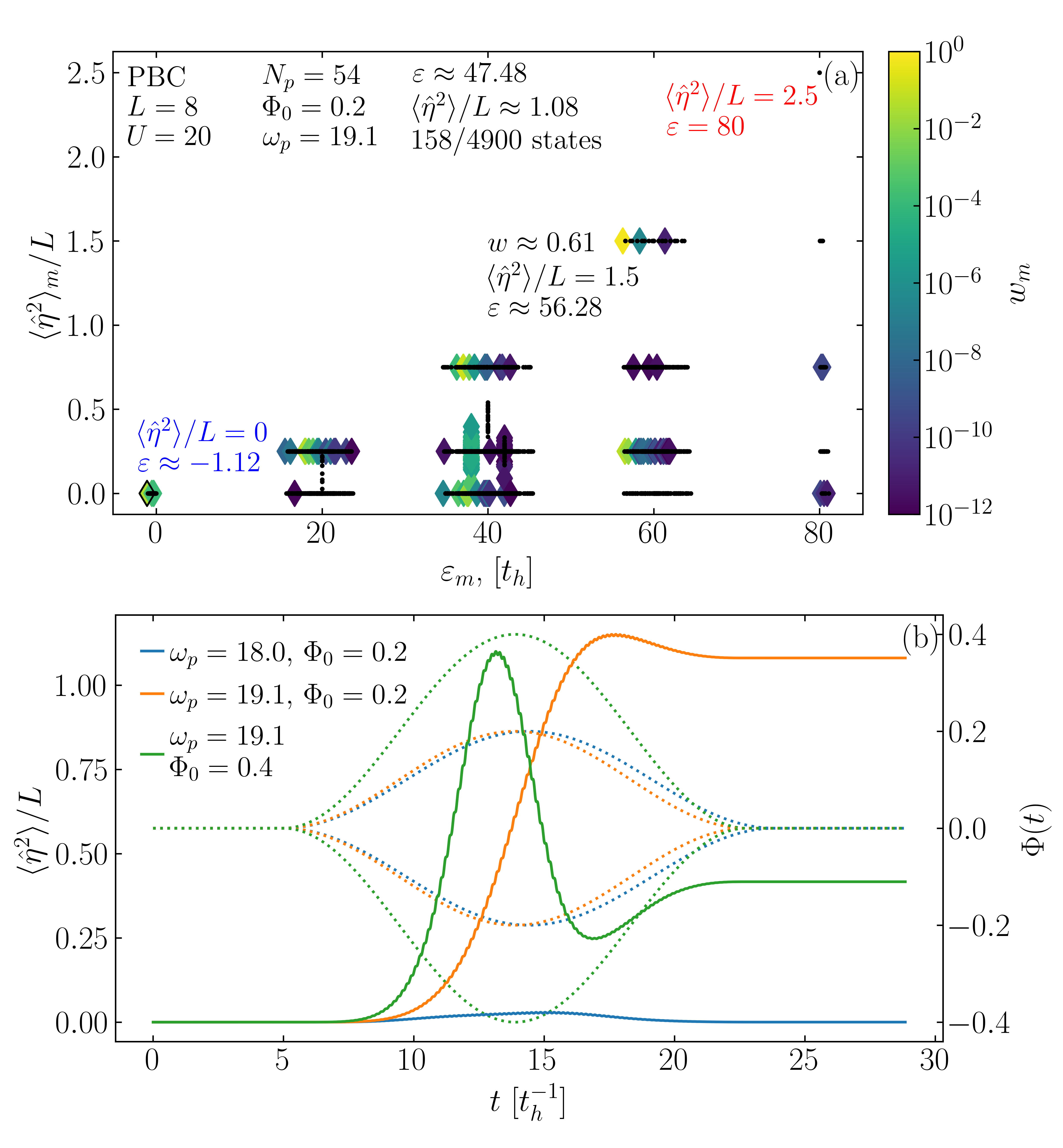
Figure 1: (a) Energy spectrum of the system (colored diamonds and black dots forming lines). The colors represent noticeable contributions of the eigenstates to the state $|\Psi_{f}\rangle$ ($w_{m}\geq 10^{-12}$) for the driving field with $\omega_{p}=19.1$ and $\Phi_{0}=0.2$ [orange line in (b)]. (b) Evolution of the order parameter $\langle\hat{\eta}^{2}\rangle/L$ driven by the pulses (4) with the respective envelopes indicated by the dotted lines.

To analyze in detail the dependence of photoexcited superconducting correlations on a pulse’s frequency and amplitude, we run a number of independent simulations for different values of $\omega_{p}$ or $\Phi_{0}$. The results of this parameter scan are summarized in Figs. 1(a) and 1(b). The maximum value of the order parameter attained is shown in Fig. 1(a). The steady-state value of the order parameter, reached after the laser pulse is turned off, is depicted in Figs. 1(b). A wide split-resonance band near $\omega_{p}\approx U=20$ and several narrow side stripes at lower frequencies can be observed, whereas no significant excitations are seen in the high-frequency regime $\omega_{p}\geq 30$.

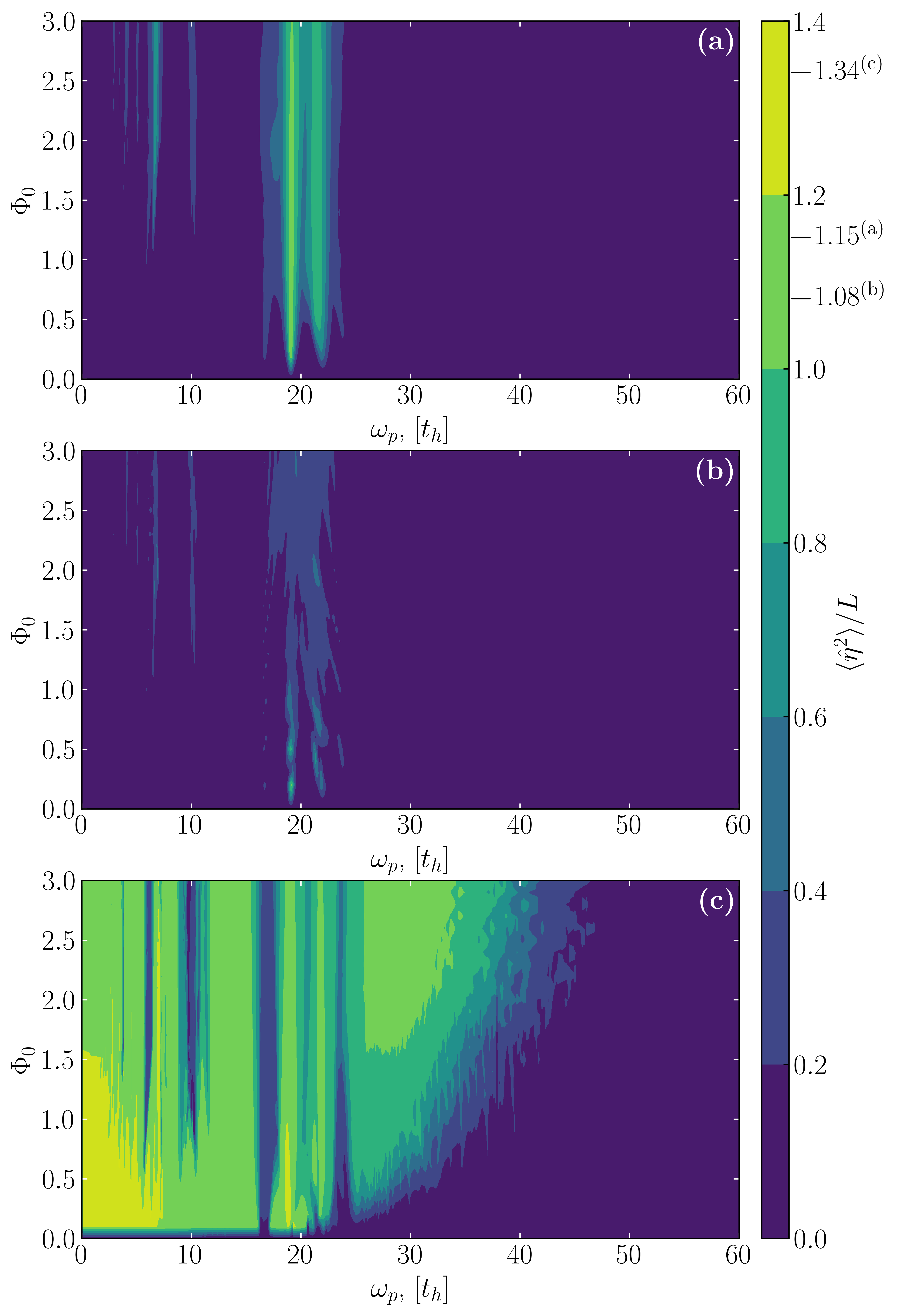
Figure 2: (a) The maximal values of the order parameter achieved during evolution as functions of the pulse parameters $\omega_{p}$ and $\Phi_{0}$ (no quantum control). (b) The saturated values of the order parameter at the end of the same simulation (no quantum control). (c) The saturated values of the order parameter after applying the Lyapunov-based quantum control (see Sec. III.1 for details). The maximal values achieved in each subfigure are indicated by the respective additional ticks in the color bar.

III Control of Superconducting correlations

III.1 Enhancing superconducting correlations with the Lyapunov quantum control

The Lyapunov quantum control [11, 12, 13, 14, 15, 16, 17], is a quantum adaptation of the celebrated Lyapunov control [30], is a feedback protocol for updating the control field to maintain a non-negative time derivative of the target property. The Ehrenfest theorem for $\hat{\eta}^{2}$ reads

$$\frac{\differential}{\differential t}\langle\hat{\eta}^{2}\rangle=i\left\langle[\hat{\mathcal{H}},\hat{\eta}^{2}]\right\rangle.$$ (6)

One obtains from Eqs. (1) and (2),

$$[\hat{\mathcal{H}},\hat{\eta}^{2}]=-it_{h}\sin[\Phi(t)]\hat{\mathcal{Q}},$$ (7)

where

$$\hat{\mathcal{Q}}=\sum_{i,j}(-1)^{i+j}\left\{\hat{c}_{i,\uparrow}^{\dagger}\hat{c}_{i+1,\downarrow}^{\dagger}-\hat{c}_{i,\downarrow}^{\dagger}\hat{c}_{i+1,\uparrow}^{\dagger},\hat{c}_{j,\uparrow}\hat{c}_{j,\downarrow}\right\}+h.c.;$$ (8)

hence,

$$\frac{\differential}{\differential t}\langle\hat{\eta}^{2}\rangle=t_{h}\sin[\Phi(t)]\langle\hat{\mathcal{Q}}\rangle.$$ (9)

The key idea behind the Lyapunov control is that with a judicious choice of $\Phi(t)$, we can ensure $\frac{\differential}{\differential t}\langle\hat{\eta}^{2}\rangle\geq 0$, thereby guaranteeing that the superconducting order parameter $\langle\hat{\eta}^{2}\rangle$ does not decrease over time. We choose the control field to be

$$\Phi^{\rm{(L)}}\Big{\{}|\Psi(t)\rangle\Big{\}}=\arcsin\frac{\langle\hat{\mathcal{Q}}\rangle}{\langle\hat{\mathcal{Q}}\rangle_{\max}}\Longrightarrow\frac{\differential}{\differential t}\langle\hat{\eta}^{2}\rangle\geq 0,$$ (10)

where $\langle\hat{\mathcal{Q}}\rangle_{\max}$ is the largest eigenvalue of $\hat{\mathcal{Q}}$ by module to ensures that the argument of $\arcsin$ is in $[-1,+1]$.

Note that it is not sufficient to just replace $\Phi(t)$ in the Hamiltonian (1) with the control pulse $\Phi^{\rm{(L)}}\{|\Psi(t)\rangle\}$ and launch the quantum evolution, since this leads to the trivial result $\Phi^{\rm{(L)}}\{|\Psi(t)\rangle\}=0$, i.e., no laser field, and $\langle\hat{\eta}^{2}\rangle=0$. Therefore, it is necessary first to excite the system with, say, a monochromatic pulse (4) followed by the Lyapunov control pulse (10). We will denote such a concatenated pulse by

$$\Phi_{\rm{L}}(t)=\begin{cases}\Phi(t)\text{ from Eq.~\eqref{eq:field}},&\text{if }t<t^{\rm{(act.)}},\\ \Phi^{\rm{(L)}}\{|\Psi(t)\rangle\},&\text{if }t\geq t^{\rm{(act.)}}.\end{cases}$$ (11)

We have empirically found that the Lyapunov protocol (10) should replace the monochromatic driving (4) when the time-derivative of the order parameter averaged over the preceding period of monochromatic field oscillations $T_{p}=2\pi/\omega_{p}$ turns negative, i.e.,

$$\left\langle\frac{\differential}{\differential t}\langle\hat{\eta}^{2}\rangle\right\rangle_{T_{p}}=\frac{t_{h}}{T_{p}}\int_{t^{\rm{(act.)}}-T_{p}}^{t^{\rm{(act.)}}}\sin[\Phi(t)]\langle\hat{\mathcal{Q}}\rangle dt<0.$$ (12)

This condition is robust to numerical noise that can manifest itself in tiny negative values of $\frac{\differential}{\differential t}\langle\hat{\eta}^{2}\rangle$. Other threshold-based conditions to turn on the Lyapunov control can also be employed, e.g., we activate $\Phi^{\rm{(L)}}\{|\Psi(t)\rangle\}$ when $\frac{\differential}{\differential t}\langle\hat{\eta}^{2}\rangle<-10^{-3}$. However, in either case, it is typical to observe an abrupt change of the control field at the switching time $t^{\rm{(act.)}}$, e.g., as can be seen in Fig. 3(a).

To demonstrate the superiority of the Lyapunov control over simple monochromatic driving, Fig. 2(c) shows the values of the superconducting order parameter reached at the end of evolution driven by the concatenated field (11) as a function of the pump pulse’s (4) frequency $\omega_{p}$ and amplitude $\Phi_{0}$ before it is replaced by the Lyapunov control pulse once the activation condition (12) is satisfied. Note that the final value of the order parameter is also the maximum value attained since the Lyapunov control ensures that the order parameter does not decrease [see Eq. (10)]. Comparing Figs. 2(b) and 2(c) reveals that the Lyapunov control becomes especially efficient at low frequencies and small amplitudes of the pump pulse.

To gain further insights into the evolution driven by the concatenated field (11) with the activation condition (12), we separately analyze in Fig. 3(a) the time evolution of $\langle\hat{\eta}^{2}\rangle$ for two monochromatic pulses from Fig. 1(b) that drive the weakest ($\omega_{p}=18.0$, $\Phi_{0}=0.2$) and strongest ($\omega_{p}=19.1$, $\Phi_{0}=0.2$) excitations of the order parameter. The solid orange and blue lines without symbols in Fig. 3(a) depict the evolutions of $\langle\hat{\eta}^{2}\rangle$ driven by monochromatic drivings (uncontrolled evolution, UE). The orange and blue solid lines with filled circles depict the evolutions of $\langle\hat{\eta}^{2}\rangle$ achieved via the Lyapunov quantum control (LQC). Not only does the Lyapunov control significantly enhance the weakest off-resonant steady-state value (blue), but it also leads to a slight increase of the previously obtained maximal value in the resonant case (orange).

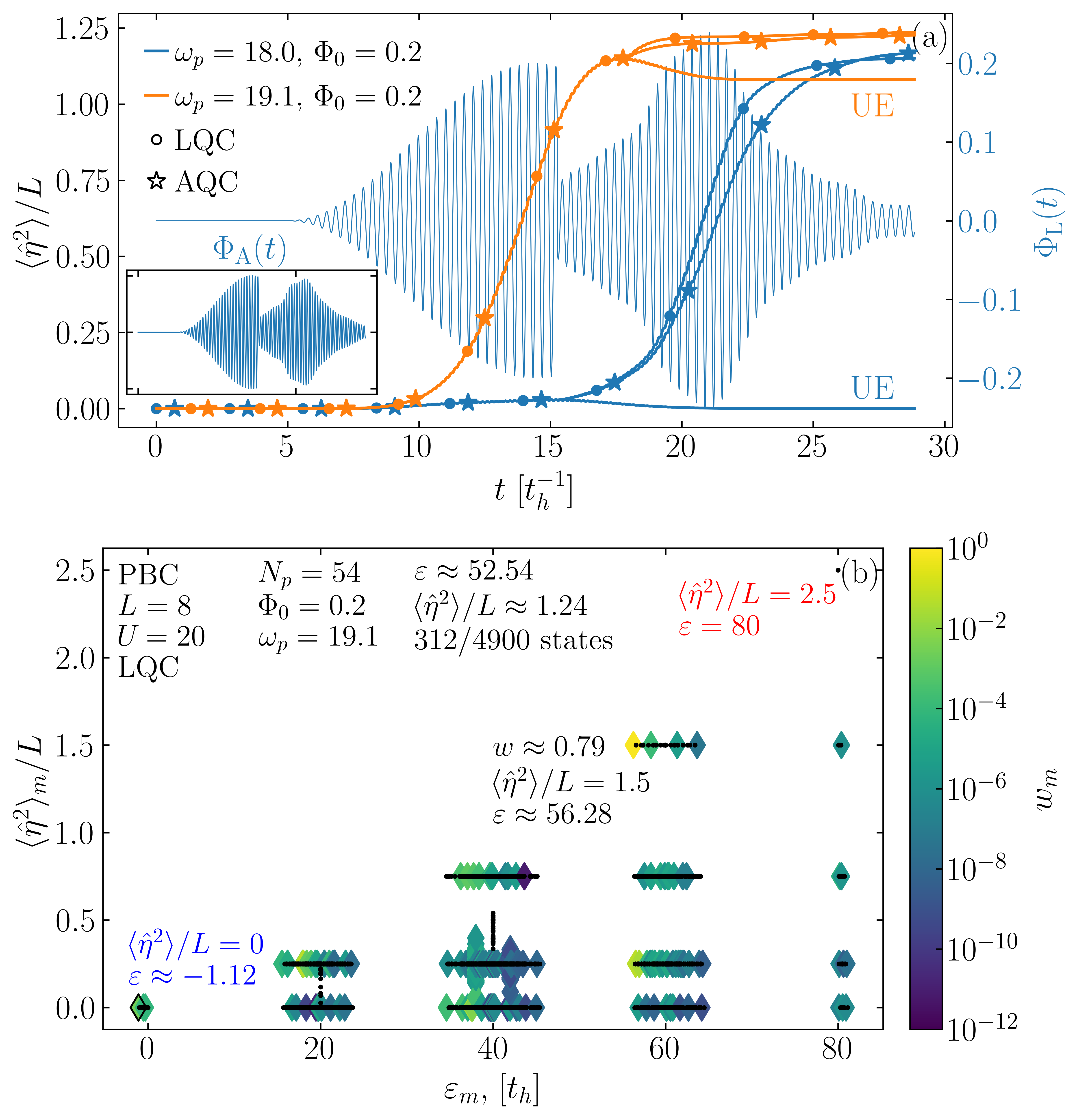
Figure 3: (a) Evolution of $\langle\hat{\eta}^{2}\rangle/L$ under $\Phi(t)$ (solid lines), $\Phi_{\rm{L}}(t)$ [filled circles (LQC)], and $\Phi_{\rm{A}}(t)$ (see Sec. III.3 for details) [stars (AQC)]. The driving fields $\Phi_{\rm{L}}(t)$ (main panel) and $\Phi_{\rm{A}}(t)$ (inset) are shown only for $\omega_{p}=18.0$. (b) The contributions of 312 eigenstates (color-coded diamond symbols) of the Hamiltonian (1) to the final state with energy $\varepsilon\approx 52.54$ and the order parameter $\langle\hat{\eta}^{2}\rangle/L\approx 1.24$ achieved during the LQC evolution for the initial field $\Phi(t)$ with $\omega_{p}=19.1$ and $\Phi_{0}=0.2$.

To understand how the Lyapunov control leads to the enhancement of the superconducting correlations in the resonant case, Fig. 3(b) [similarly to Fig. 1(a)] depicts the population of eigenstates (3) at the end of the dynamics driven by the concatenated pulse (11) with $\omega_{p}=19.1$ and $\Phi_{0}=0.2$ for the initial monochromatic pump pulse $\Phi(t)$. As in Fig. 1(a), $w_{m}=|\langle\psi_{m}|\Psi_{f}\rangle|^{2}$ is obtained from Eq. (5), where $\ket{\Psi_{f}}$ is the final state. Comparing the outcome of the pure monochromatic driving [Fig. 1(a)] with the Lyapunov control [Fig. 3(b)], we observe that for the Lyapunov control twice as many eigenstates have $w_{m}\geq 10^{-12}$; additionally, the eigenstate with $\langle\hat{\eta}^{2}\rangle/L=1.5$ and $\varepsilon_{m}\approx 56.28$ has increased its population to above 75%. Surprisingly, no contribution is observed from the eigenstate with the largest-possible order parameter [see the black dot at the upper right corner of Fig. 3(b) as well as Fig. 1(a)].

It is important to observe from Fig. 3(a) that the carrier frequency of the introduced Lyapunov pulse $\Phi^{\rm{(L)}}\{|\Psi(t)\rangle\}$ is close to the frequency of the preceding monochromatic pump $\Phi(t)$. This increases the prospects of experimental implementations of the Lyapunov control as it is easier to realize the modulation of the envelope (see, e.g., Ref. [31]).

III.2 When is it best to activate the Lyapunov control?

The evolution induced by the concatenated field (11) depends on the activation time $t^{\rm{(act.)}}$ – when the monochromatic field is replaced by the Lyapunov control. Up to this point, the activation time $t^{\rm{(act.)}}$ was chosen by the condition (12). However, Fig. 2(c) contains many examples where such a switching condition does not enhance the order parameter (see, in particular, the case of the pump pulse with $\omega_{p}=17.0$ and $\Phi_{0}=0.4$). Nevertheless, changing $t^{\rm{(act.)}}$ improves the steady-state value of the order parameter. The red curve ($\rm{LQC^{(sat.)}}$) in the main panel of Fig. 4(a) depicts the steady state value of $\langle\hat{\eta}^{2}\rangle$ as a function of $t^{\rm{(act.)}}$ for the pump pulse with $\omega_{p}=17.0$ and $\Phi_{0}=0.4$.

Recall that from Figs. 1 and 3, it followed that the monochromatic excitation with $\omega_{p}=19.1$ and $\Phi_{0}=0.2$ yielded a high value of the order parameter. In such a case, the value of the order parameter $\langle\hat{\eta}^{2}\rangle$ reached at the end of the evolution driven by the concatenated pulse (11) as a function of the activation time $t^{\rm{(act.)}}$, shown in the inset of Fig. 4(a), reveals considerable freedom in choosing $t^{\rm{(act.)}}$. Note that in both cases analyzed in Fig. 4(a), it is sufficient to turn on the Lyapunov control just after a few oscillations of the initial pump field to achieve a significant amplification of the superconducting order parameter. This seems natural since activating the control earlier provides more time for the development of superconducting correlations.

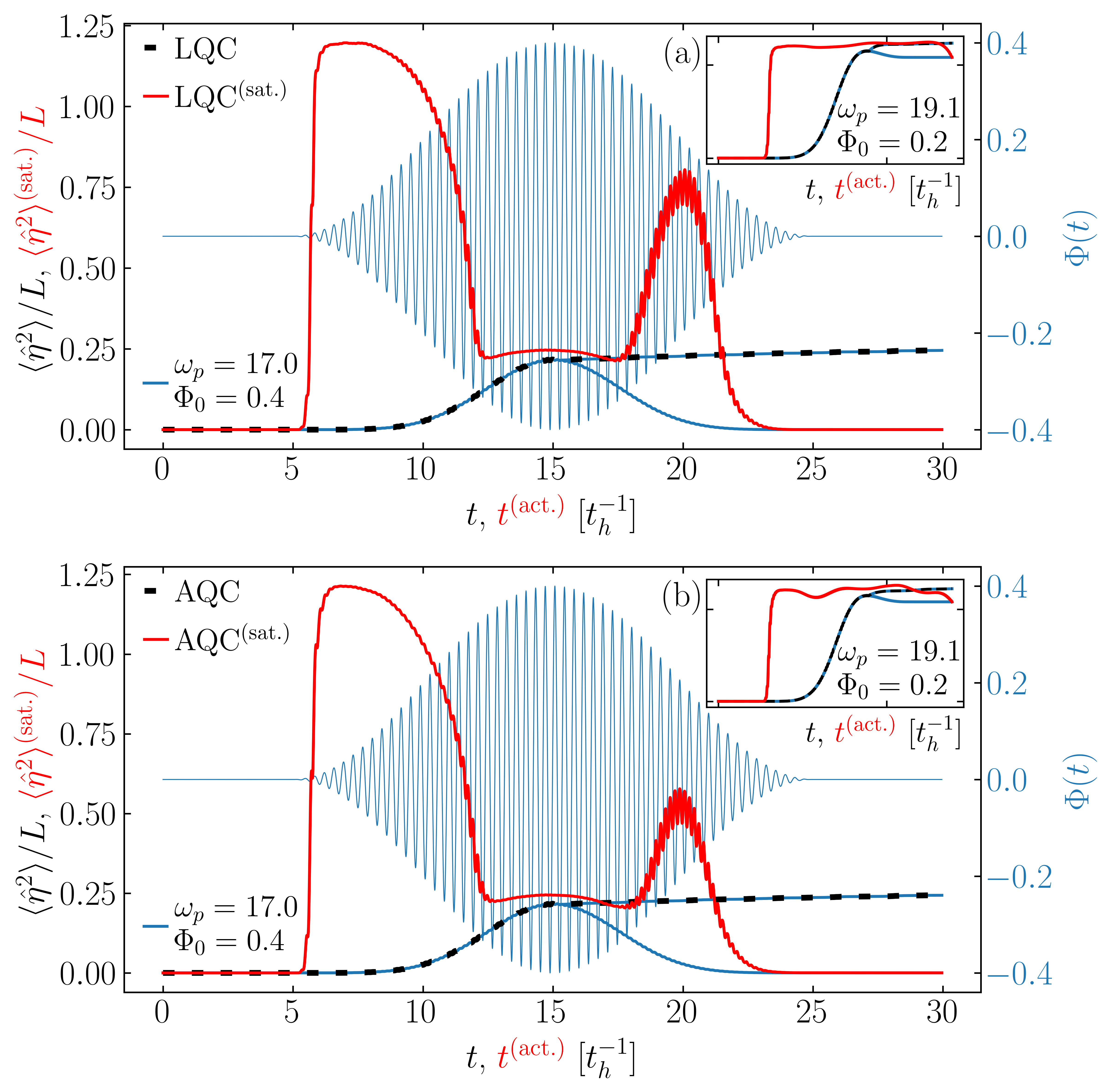
Figure 4: (a) The saturated value of $\langle\hat{\eta}^{2}\rangle/L$ with respect to activation time $t^{\rm{(act.)}}$ [red curves ($\rm{LQC^{(sat.)}}$)] along with the evolution of $\langle\hat{\eta}^{2}\rangle/L$ driven by $\Phi(t)$ (blue lines) and $\Phi_{\rm{L}}(t)$ with switching condition (12) [black dashed line (LQC)]. The uncontrolled driving field is shown only in the main panel ($\omega_{p}=17.0$, $\Phi_{0}=0.4$), the results in the inset correspond to $\omega_{p}=19.1$, $\Phi_{0}=0.2$. (b) The same quantities as in (a), but red solid ($\rm{AQC^{(sat.)}}$) and black dashed lines correspond to asymptotic quantum control (AQC, see Sec. III.3).

III.3 Asymptotic quantum control

The maximum possible value of the superconducting order parameter is $\langle\hat{\eta}^{2}\rangle_{\max}/L=(L/2+1)/2=2.5$, yet the most we have got so far is $\langle\hat{\eta}^{2}\rangle/L\approx 1.34$ [see Fig. 2(c)]. It is tempting to modify the Lyapunov control protocol to see if $\langle\hat{\eta}^{2}\rangle_{\max}$ can be reached.

Let us introduce the asymptotic quantum control (AQC). Unlike the Lyapuniv control (9) that aims to increase $\langle\hat{\eta}^{2}\rangle$, AQC tends to decrease the difference between $\langle\hat{\eta}^{2}\rangle$ and some chosen target value $\eta_{0}^{2}$, which can be set to $\langle\hat{\eta}^{2}\rangle_{\max}$. Since

$$\frac{\differential}{\differential t}\left(\langle\hat{\eta}^{2}\rangle-\eta^{2}_{0}\right)^{2}=2\left(\langle\hat{\eta}^{2}\rangle-\eta^{2}_{0}\right)t_{h}\sin[\Phi(t)]\langle\hat{\mathcal{Q}}\rangle,$$ (13)

to ensure that this derivative is non-positive, it is sufficient to choose the control $\Phi(t)$ in the form

$$\Phi^{\rm{(A)}}\Big{\{}|\Psi(t)\rangle\Big{\}} =-\arcsin\frac{\langle\hat{\mathcal{Q}}\rangle\left(\langle\hat{\eta}^{2}\rangle-\eta^{2}_{0}\right)}{\langle\hat{\mathcal{Q}}\rangle_{\max}\langle\hat{\eta}^{2}\rangle_{\max}}$$ (14)

$$\Longrightarrow\frac{\differential}{\differential t}\left(\langle\hat{\eta}^{2}\rangle-\eta^{2}_{0}\right)^{2}\leq 0,$$

where $\langle\hat{\mathcal{Q}}\rangle_{\max}$ and $\langle\hat{\eta}^{2}\rangle_{\max}$ are the largest eigenvalues by module of $\hat{\mathcal{Q}}$ and $\hat{\eta}^{2}$, respectively, to ensures that the argument of $\arcsin$ is in $[-1,+1]$.

As in the case of LQC, we start the evolution from the ground state for which $\langle\hat{\mathcal{Q}}\rangle=0$, hence an initial monochromatic pump pulse is needed to kick the dynamics. Also, we need to choose the activation time $t^{\rm{(act.)}}$ when the pump should be replaced by the asymptotic control (14). The activation condition (12), employed in Sec. III.1, leads to very similar results in the case of AQC, as shown in Fig. 3(a). As shown in the inset of Fig. 3(a), the resulting concatenated field

$$\Phi_{\rm{A}}(t)=\begin{cases}\Phi(t)\text{ from Eq.~\eqref{eq:field}},&\text{if }t<t^{\rm{(act.)}},\\ \Phi^{\rm{(A)}}\{|\Psi(t)\rangle\},&\text{if }t\geq t^{\rm{(act.)}},\end{cases}$$ (15)

is very similar to $\Phi_{\rm{L}}(t)$ [Eq. (11)]. Also, the dependence of the final value of $\langle\hat{\eta}^{2}\rangle$ on the parameters of the pump pulse is almost identical to the one attained by the Lyapunov control as shown in Fig. 2(c).

Finally, AQC leads to a marginal improvement of the final maximum value of the order parameter $\langle\hat{\eta}^{2}\rangle/L\approx 1.37$ over the Lyapunov control result of $\langle\hat{\eta}^{2}\rangle/L\approx 1.34$, still significantly falling short of $\langle\hat{\eta}^{2}\rangle_{\max}$. Perhaps to further increase the superconducting correlations, one needs to resort to a much more computationally expensive approach of optimal quantum control, which, unlike both the Lyapunov and asymptotic controls, typically requires a large number of iterations to converge the unknown control.

We should note that the excitability of superconducting correlations depends more strongly on the switching condition determining $t^{\rm{(act.)}}$ (see Sec. III.2) than on the specific type of the employed quantum control, i.e., LQC or AQC. Similarly to the Lyapunov quantum control, asymptotic control does not make condition (12) effective for the monochromatic pump pulse with $\omega_{p}=17.0$ and $\Phi_{0}=0.4$. Figure 4(b) (main panel) shows the dependence of the saturated value of $\langle\hat{\eta}^{2}\rangle/L$ on $t^{\rm{(act.)}}$ (red solid line) in the case of AQC [cf. Fig. 4(a)].

III.4 Tracking quantum control

The discussed quantum controls did not lead to excitation of the state with the maximal value $\langle\hat{\eta}^{2}\rangle/L=2.5$. If one only needs the current response of a system excited to the maximum order parameter, it turns out that one can do it without bringing the system to such a state. Tracking quantum control with easily fulfilled conditions allows one to obtain the required current response from the system in its ground state, making the system mimic an alien response. The application of this quantum control has been studied in detail for the metallic and Mott insulating states of the Fermi-Hubbard model in the preceding studies [32, 33, 34, 35, 36]. Their results can be directly applied to the many-body states with superconducting correlations being the focus of the current study.

III.5 Suppressing superconducting correlations with the Lyapunov quantum control

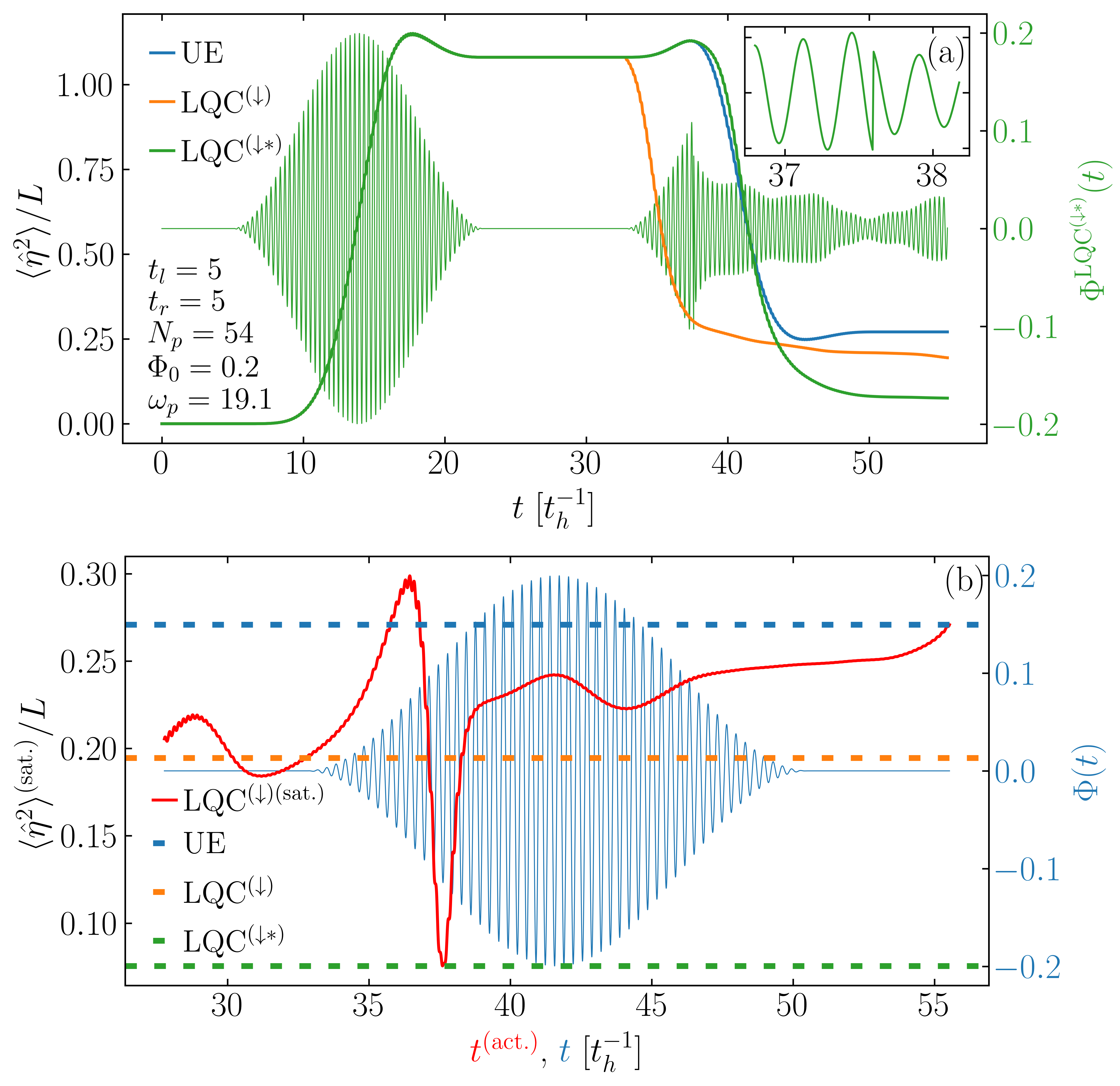
Figure 5: (a) Excitation and consequent suppression of the superconducting correlations with $\Phi^{\rm(UE)}(t)$ from Eq. (17) (labeled UE), $\Phi^{\rm{LQC^{(\downarrow)}}}(t)$ from Eq. (18) ($\rm{LQC^{(\downarrow)}}$), and $\Phi^{\rm{LQC^{(\downarrow*)}}}(t)$ with the optimal $t^{\rm{(act.)}}$ ($\rm{LQC^{(\downarrow*)}}$). Parameters are $\omega_{p}=19.1$ and $\Phi_{0}=0.2$. (b) The saturated value of $\langle\hat{\eta}^{2}\rangle/L$ as a function of $t^{\rm{(act.)}}$ (red line) and the saturated values reached in UE, $\rm{LQC^{(\downarrow)}}$, and $\rm{LQC^{(\downarrow*)}}$ evolutions (dashed lines).

In Sec. III.1, we have established that the Lyapunov quantum control enhances superconducting correlations. We now demonstrate that the opposite can also be achieved—the suppression of superconducting correlations, thereby enabling almost full on-demand control of quantum correlations.

From Eq. (9), it readily follows that the following control accomplishes the suppression of superconductivity:

$$\Phi^{\downarrow}\Big{\{}|\Psi(t)\rangle\Big{\}}=-\arcsin\frac{\langle\hat{\mathcal{Q}}\rangle}{\langle\hat{\mathcal{Q}}\rangle_{\max}}\Longrightarrow\frac{\differential}{\differential t}\langle\hat{\eta}^{2}\rangle\leq 0.$$ (16)

Note that the controls for enhancing [Eq. (10)] and suppressing [Eq. (16)] the correlations differ only by sign.

To benchmark the Lyapunov control for suppressing superconductivity, we first illustrate the effect of monochromatic driving. We take the pump pulse $\Phi(t)$ from Eq. (4) with parameters $\omega_{p}=19.1$ and $\Phi_{0}=0.2$. This pulse yields $\langle\hat{\eta}^{2}\rangle/L\approx 1.08$ – the largest value of the steady-state of the order parameter attained in Fig. 1(b). The blue line (labeled UE) in Fig. 5(a) shows the evolution of the order parameter when the pulse $\Phi(t)$ is applied twice resulting in the field

$$\Phi^{\rm(UE)}(t)=\Phi(t)+\Phi(t-{\Delta t}),$$ (17)

The first pulse induces the superconductive correlations. When the second identical pulse is applied at a later time ($\Delta t=t_{l}+t_{r}+T_{p}N_{p}$, where $t_{l}$ and $t_{r}$ is the idle time before and after the pulse, respectively), the order parameter decreases to $\langle\hat{\eta}^{2}\rangle/L\approx 0.25$ and ultimately settles at $\langle\hat{\eta}^{2}\rangle/L\approx 0.27$.

As illustrated by the orange line (labeled $\rm{LQC^{(\downarrow)}}$) in Fig. 5(a), the following Lyapunov control allows us to further decrease $\langle\hat{\eta}^{2}\rangle/L\approx 0.19$:

$$\Phi^{\rm{LQC^{(\downarrow)}}}(t)=\begin{cases}\Phi^{\rm(UE)}(t)\text{ from Eq.~\eqref{eq:PhiUE}},&\text{if }t<t^{\rm{(act.)}},\\ \Phi^{\downarrow}\Big{\{}|\Psi(t)\rangle\Big{\}},&\text{if }t\geq t^{\rm{(act.)}},\end{cases}$$ (18)

where the activation time $t^{\rm{(act.)}}$ of the Lyapunov suppressing control (16) is chosen such that

$$t^{\rm{(act.)}}\geq{\Delta t},\qquad\int_{t^{\rm{(act.)}}-T_{p}}^{t^{\rm{(act.)}}}\sin[\Phi(t)]\langle\hat{\mathcal{Q}}\rangle dt>0.$$ (19)

Note that the latter condition is directly inspired by Eq. (12).

However, we can push the order parameter even further down to $\langle\hat{\eta}^{2}\rangle/L\approx 0.08$. The final value of $\langle\hat{\eta}^{2}\rangle$ achieved strongly depends on the choice of the activation time $t^{\rm{(act.)}}$. This dependency is visualized by the red curve in Fig. 5(b). The minimum of the red curve gives the optimal choice of the activation time. The control field (18) with such a choice of $t^{\rm{(act.)}}$ yields $\langle\hat{\eta}^{2}\rangle/L\approx 0.08$. The full time evolution of the order parameter is shown as the green curve (labeled $\rm{LQC^{(\downarrow*)}}$) in Fig. 5(a). Note that the order parameter first reaches a maximum before the descent. This strong suppression comes at the cost of an abrupt change in the control field at the activation time, as shown in the inset of Fig. 5(a).

IV Conclusion

We have demonstrated that Lyapunov quantum control provides an effective method for enhancing superconducting correlations in the one-dimensional Fermi-Hubbard model without requiring intricate fine-tuning of pulse parameters. Our key findings include: First, traditional monochromatic driving only excites superconducting correlations within narrow frequency ranges, making it challenging to optimize without extensive parameter searches. In contrast, Lyapunov control efficiently amplifies even weakly excited states, particularly at low frequencies and amplitudes of the initial pumping field.

Second, our approach eliminates the need for precise pulse engineering by automatically shaping the field envelope while maintaining the carrier frequency. This makes experimental implementation more feasible. Third, we showed that a variant of this approach—asymptotic quantum control—yields comparable enhancement of superconducting correlations, confirming the robustness of time-local control methods for this application. Finally, we demonstrated that Lyapunov control can also be used to effectively suppress previously induced superconducting correlations, enabling bidirectional control of quantum correlations on demand. These results highlight the potential of Lyapunov quantum control as a practical tool for manipulating superconducting properties in strongly correlated electron systems.