Yan Liu${}^{\,a,b}$, Chuan-Yi Wang${}^{\,a,b}$ and You-Jie Zeng${}^{\,a,b}$

^aCenter for Gravitational Physics, Department of Space Science,
Beihang University, Beijing 100191, China

^bPeng Huanwu Collaborative Center for Research and Education,
Beihang University, Beijing 100191, China

Energy transport in holographic
non-conformal interfaces

1 Introduction

Interfaces arise in diverse physical systems, including the impurities in samples, quantum wire junctions, waveguide systems, surface phenomena in statistical mechanics, and edge modes of topologically ordered systems. Meanwhile, interfaces play crucial roles in the ambient theory, such as Wilson loops probing the phases of gauge theory, $D$-branes in string theory etc. Therefore, characterizing the properties of interfaces is of significant interest across diverse fields.

When a codimension one interface preserves half of the conformal symmetry, it is termed a conformal interface. In two dimensions, conformal interfaces have attracted substantial research attention. Various physical quantities, such as interface entropy or the $g$-function [1], effective central charge [2], and energy transport [3, 4], have been extensively explored. These quantities are generally distinct but may be interrelated through simple inequalities [5]. This paper focuses on energy transports across the interface.

Energy transports are key quantities that characterize the transmission or reflection of energy across an interface. Here, we study a specific case where the two CFTs separated by the interface possess the same central charge, which share similarities as the system of defects or impurities [6, 7, 8, 9]. When a pulse of energy is sent from the left side, the transmitted energy to the right is proportional to a coefficient $\mathcal{T}$, and the reflected portion is proportional to $\mathcal{R}$, with $\mathcal{T}+\mathcal{R}=1$ in the absence of absorption. This process is governed by the two-point function of the energy-momentum tensor across the interface [4].

It has been established in [3] the transmission coefficient $\mathcal{T}$ and reflection coefficient $\mathcal{R}$ fall within the interval $[0,1]$ for conformal interfaces in a class of unitary CFTs, while they break these bounds for nonunitary CFTs. The relation $\mathcal{T}+\mathcal{R}=1$ always holds. For ICFT, similar results were derived from averaged null-energy condition [4]. In strongly coupled systems, the AdS/CFT correspondence proves useful [10, 11]. For holographic ICFTs, which are dual to a gravitational system consists of two AdS₃ regions with the same cosmological constant separated by an interface brane with tension $\sigma$, the transmission coefficient is given by $\mathcal{T}=\left(1+4\pi GL\sigma\right)^{-1}$ and $\mathcal{R}=1-\mathcal{T}$ [12]. These findings were further confirmed in a study of holographic non-equilibrium steady states with an interface brane [13]. Given that the tension $\sigma$ is constrained to $[0,1/(4\pi GL)]$ in AdS/ICFT, new constraints $\frac{1}{2}\leq\mathcal{T}\leq 1\,,$ were discovered [12]. The permissible range of transmission coefficient can be further tunned from $0$ to $1$ in double brane holographic models [14] and Janus configurations [15]. Further studies on the energy transports in AdS/ICFT can be found in [16, 17, 18, 19, 20].

The goal of this paper is to extend beyond conformal interfaces and investigate energy transport in scenarios with generic interfaces. We consider a setup where the interface hosts a localized scalar degree of freedom. In the holographic context, the bulk system is composed of the left half AdS₃ and the right half AdS₃, joined by an interface brane on which a scalar filed is localized. This configuration was previously analyzed in [21], where the properties of brane configurations and $g$-functions were systematically investigated, revealing that both the interface entropy and the $g$-functions manifest explicit scale dependence, which directly indicates the symmetry breaking of conformal interface induced by the localized scalar operator. Thus this setup serves as a holographic model for non-conformal interfaces. In this work, we focus on the case of ICFT with identical central charges on both sides of the interface for simplicity, and examine energy transport across the non-conformal interface.

This paper is organized as follows. In section 2, we review the construction of AdS/ICFT for a non-conformal interface and analyze the perturbations of the system. In section 3, we first discuss the boundary conditions necessary to obtain the energy transport and then study the properties of the transmission coefficients in various examples to identify universal behaviors. Finally, in section 4 we summarize our findings and discuss open questions. Appendix A provides useful equations used in the main text, and appendix B briefly reproduces the results for the energy transport in conformal interface.

2 Holographic model of non-conformal interface

In this section, we first review the holographic model for a two-dimensional strongly coupled field theory with a non-conformal interface [21], where a localised scalar operator appears at the interface. We set the left and right CFT of the interface to have the same central charge, resulting in the entire system resembling a holographic model for a defect. Then we analyze the linear fluctuations of the system.

The gravitational theory is described by the following action,

$$S_{\text{bulk}}=S_{\text{I}}+S_{\text{II}}+S_{Q}$$ (2.1)

where

$$\begin{split}S_{\text{I}}&=\int_{N_{\text{I}}}d^{3}x\sqrt{-g_{\text{I}}}\,\bigg{[}\frac{1}{16\pi G}\bigg{(}R_{\text{I}}+\frac{2}{L_{\text{I}}^{2}}\bigg{)}\bigg{]},\\ S_{\text{II}}&=\int_{N_{\text{II}}}d^{3}x\sqrt{-g_{\text{II}}}\,\bigg{[}\frac{1}{16\pi G}\bigg{(}R_{\text{II}}+\frac{2}{L_{\text{II}}^{2}}\bigg{)}\bigg{]},\\ S_{Q}&=\frac{1}{8\pi G}\int_{Q}d^{2}y\sqrt{-h}\,\bigg{[}\big{(}K_{\text{I}}-K_{\text{II}}\big{)}-(\partial\phi)^{2}-V(\phi)\bigg{]}.\end{split}$$ (2.2)

The coordinates on $N_{\text{I}}$ ($N_{\text{II}}$) are $x_{\text{I}}^{a}=(u_{\text{I}},t_{\text{I}},x_{\text{I}})$ ($x_{\text{II}}^{a}=(u_{\text{II}},t_{\text{II}},x_{\text{II}})$). We choose the AdS boundary of $N_{\text{I}}$ to lie in the region $x_{\text{I}}<0$ while boundary of $N_{\text{II}}$ is in the region $x_{\text{II}}>0$. The boundary of interface brane $Q$ is located at $x_{\text{I}}=x_{\text{II}}=0$. Assuming the coordinates on $Q$ are $y^{\mu}=(t,z)$, the profile of the brane $Q$ in the bulk is parameterized by $x_{\text{I}}^{a}=x_{\text{I}}^{a}(y^{\mu})$ and $x_{\text{II}}^{a}=x_{\text{II}}^{a}(y^{\mu})$. The continuous condition of the metric on $Q$, as well as the equation of motion on $Q$, constrain the permissible embeddings. The equations of motion for the system can be found in appendix A.1.

Here, we assume that CFT${}_{\text{I}}$ and CFT${}_{\text{II}}$ have identical central charge, i.e. $L_{\text{I}}=L_{\text{II}}=L$. The interface in the field theory can be thought as a defect or impurity within the system. We focus on the zero-temperature system. The bulk geometry for $N_{\text{I}}$ and $N_{\text{II}}$ is the planar AdS₃ solution

$$ds^{2}_{A}=\frac{L^{2}}{u_{A}^{2}}\bigg{[}-dt_{A}^{2}+dx^{2}_{A}+du_{A}^{2}\bigg{]}\,,~~~A=\text{I\,,~~II}\,.$$ (2.3)

We have the equation for $Q$ as

$$x_{\text{I}}=\psi(z)\,,~~~x_{\text{II}}=-\psi(z)$$ (2.4)

and the equations of motion for the scalar field or equivalently the null energy condition constraints $\psi^{\prime\prime}(z)\leq 0$.

For the equilibrium configuration, we have the solution with $t_{\text{I}}=t_{\text{II}}=t,~u_{\text{I}}=u_{\text{II}}=z$. The resulting equations are

$$\phi^{\prime 2}=-\frac{L\,\psi^{\prime\prime}}{2z\sqrt{1+\psi^{\prime 2}}}\,,~~~V(\phi)=\frac{2\psi^{\prime}(1+\psi^{\prime 2})-z\psi^{\prime\prime}}{2L(1+\psi^{\prime 2})^{3/2}}\,.$$ (2.5)

These equations are the same as the configuration in BCFT setup, and the ICFT could be understood as an unfold of BCFT at the leading order [22, 21]. In the following, we consider the linear fluctuations of the entire system and derive the energy transport from the fluctuations.

2.1 Solution at first order and energy transport

To compute the holographic transport coefficient, we consider the first order perturbation of the equation of motion. The first order perturbation of the bulk metric on the left and right halves of the bulk is given by

$$ds^{2}=ds^{2}_{A}+[ds^{2}]^{(2)}_{A}\,,~~~~~~A=\text{I\,,~~II}\,$$ (2.6)

where

$$\begin{split}&[ds^{2}]^{(2)}_{\text{I}}=4GL\epsilon\left[e^{i\omega(t_{\text{I}}-x_{\text{I}})}(dt_{\text{I}}-dx_{\text{I}})^{2}+\mathcal{R}e^{i\omega(t_{\text{I}}+x_{\text{I}})}(dt_{\text{I}}+dx_{\text{I}})^{2}\right]+c.c.\,,\\ &[ds^{2}]^{(2)}_{\text{II}}=4GL\epsilon\mathcal{T}e^{i\omega(t_{\text{II}}-x_{\text{II}})}(dt_{\text{II}}-dx_{\text{II}})^{2}+c.c.\,.\end{split}$$ (2.7)

Here, $\mathcal{R},\mathcal{T}$ are the relative amplitudes of the reflected and transmitted waves, respectively, and are referred to as the reflection and transmission coefficients for convenience. Their precise physical meaning will be explained in detail in the following. The term $c.c.$ denotes complex conjugation.

From the dictionary of AdS/CFT, the dual energy momentum tensor is given by

$$T_{\alpha\beta}=\frac{1}{4GL}g_{\alpha\beta}^{(2)}\,.$$ (2.8)

Thus, the injected, reflected, and transmitted energy fluxes are

$$T_{\text{in}}/\epsilon=e^{i\omega(t_{\text{I}}-x_{\text{I}})}+c.c.\,,~~T_{\text{re}}/\epsilon=\mathcal{R}e^{i\omega(t_{\text{I}}+x_{\text{I}})}+c.c.\,,~~T_{\text{tr}}/\epsilon=\mathcal{T}e^{i\omega(t_{\text{II}}-x_{\text{II}})}+c.c.\,.$$ (2.9)

At the location of the interface $x_{\text{I}}=x_{\text{II}}=0$, the conservation of energy $T_{\text{in}}=T_{\text{re}}+T_{\text{tr}}$ can be rewritten as $(\mathcal{R}+\mathcal{T}-1)e^{i\omega t_{\text{I}}}+c.c.=0\,.$ This relation implies

$$\mathcal{R}+\mathcal{T}=1\,.$$ (2.10)

In general, $\mathcal{R},\mathcal{T}$ are complex and depend on $\omega$. Among the four real components of $\mathcal{R},\mathcal{T}$, only two are independent due to the constraint in Eq. (2.10).

The coefficients can be expressed in the form of

$$\mathcal{R}=|\mathcal{R}|e^{i\phi_{r}}\,,~~~\mathcal{T}=|\mathcal{T}|e^{i\phi_{t}}\,.$$ (2.11)

From (2.9), it is evident that the phases differ among the injected, reflected and transmitted waves, analogous to the behavior of electromagnetic waves at the interface of different media. Since $\mathcal{R},\mathcal{T}$ are generally complex, the reflection and transmission ratios are defined as,

$$\begin{split}\tilde{\mathcal{R}}&=\frac{\text{reflected energy flux}}{\text{injected energy flux}}=\frac{T_{\text{re}}}{T_{\text{in}}}=\frac{|\mathcal{R}|\cos(\omega t+\phi_{r})}{\cos(\omega t)}\,,\\ \tilde{\mathcal{T}}&=\frac{\text{transmitted energy flux}}{\text{injected energy flux}}=\frac{T_{\text{tr}}}{T_{\text{in}}}=\frac{|\mathcal{T}|\cos(\omega t+\phi_{t})}{\cos(\omega t)}\,.\end{split}$$ (2.12)

These ratios are both frequency- and time-dependent. From (2.10), we have

$$\tilde{\mathcal{R}}+\tilde{\mathcal{T}}=1\,.$$ (2.13)

Several observations can be made:

• When $\mathcal{R},\mathcal{T}$ are real (i.e. $\phi_{r}=\phi_{t}=0$), we have

  $$\tilde{\mathcal{R}}=\mathcal{R}\,,~~~\tilde{\mathcal{T}}=\mathcal{T}\,.$$ (2.14)

  They are interpreted as the reflection and transmission coefficients for conformal interface [12]. However, in general, they are complex, and a phase shift occurs in the energy fluxes.

• The instantaneous values of $\tilde{\mathcal{R}},\tilde{\mathcal{T}}$ depend on the phase $\omega t$ of the injected wave at the interface. When $\omega t=(n+\frac{1}{2})\pi$ for integer $n$, at the interface the injected wave $\langle T_{\text{in}}\rangle=2\epsilon\cos(\omega t)=0$, and $\langle T_{\text{re}}\rangle=\langle T_{\text{tr}}\rangle$.

• It is convenient to decompose the coefficients as

  $$\mathcal{R}=\mathcal{R}^{\prime}+i\mathcal{R}^{\prime\prime}\,,~~~~\mathcal{T}=\mathcal{T}^{\prime}+i\mathcal{T}^{\prime\prime}$$ (2.15)

  where $\mathcal{R}^{\prime},\mathcal{R}^{\prime\prime},\mathcal{T}^{\prime},\mathcal{T}^{\prime\prime}$ are real and satisfy

  $$\mathcal{R}^{\prime}+\mathcal{T}^{\prime}=1\,,~~~~\mathcal{R}^{\prime\prime}+\mathcal{T}^{\prime\prime}=0\,.$$ (2.16)

  From (2.12), the reflection and transmission ratios become

  $$\tilde{\mathcal{R}}=\mathcal{R}^{\prime}-\mathcal{R}^{\prime\prime}\tan(\omega t)\,,~~~\tilde{\mathcal{T}}=\mathcal{T}^{\prime}-\mathcal{T}^{\prime\prime}\tan(\omega t)\,.~~~$$ (2.17)

  We define the averaged transmission and reflection coefficients by performing the principle integration from $-\frac{\pi}{2\omega}$ to $\frac{\pi}{2\omega}$,

  $$\begin{split}\langle\tilde{\mathcal{R}}\rangle=\mathcal{R}^{\prime}\,,~~~~\langle\tilde{\mathcal{T}}\rangle=\mathcal{T}^{\prime}\,.~~~~\end{split}$$ (2.18)

  In the low frequency limit, the integration region becomes sufficiently long such that the measured quantities align with the average values.

2.1.1 The equations of perturbations

In this subsection, we show a detailed procedure for calculating the coefficients (2.7) using holography. We focus on the fluctuation of the interface brane that glues the left and right bulk together. By solving the resulting equations with appropriate boundary conditions, we derive the transport coefficients.

We adopt the following coordinate on $Q$

$$t=\frac{1}{2}(t_{\text{I}}+t_{\text{II}})\,,~~~z=\frac{1}{2}(u_{\text{I}}+u_{\text{II}})\,.$$ (2.19)

These gauge conditions are the same as those were used in [23]. The above gauge fixings reduce two of the six worldsheet diffeomorphisms of the interface brane. The perturbed brane is then parameterized as

$$\begin{split}&t_{\text{I}}=t+\frac{G\epsilon}{L}e^{i\omega\tau}\lambda(z)+c.c.\,,\ x_{\text{I}}=p(z)+\frac{2G\epsilon}{L}e^{i\omega\tau}h_{\text{I}}(z)+c.c.\,,\ u_{\text{I}}=z+\frac{2G\epsilon}{L}e^{i\omega\tau}\xi(z)+c.c.\,,\\ &t_{\text{II}}=t-\frac{G\epsilon}{L}e^{i\omega\tau}\lambda(z)+c.c.\,,\ x_{\text{II}}=-p(z)+\frac{2G\epsilon}{L}e^{i\omega\tau}h_{\text{II}}(z)+c.c.\,,\ u_{\text{II}}=z-\frac{2G\epsilon}{L}e^{i\omega\tau}\xi(z)+c.c.\,,\end{split}$$ (2.20)

and the perturbed scalar is given by

$$\phi(z)=\phi_{bg}(z)+4G\epsilon\,e^{i\omega t}p(z)+c.c.$$ (2.21)

where $t$ and $z$ are the intrinsic coordinates of the brane, and $\phi_{bg}(z)$ is the background scalar field. Note that the above perturbations break spatial inversion symmetry.

The system has five independent perturbed fields, i.e. $\lambda(z),h_{\text{I}}(z),h_{\text{II}}(z),\xi(z),$ $p(z)$. Substituting these fluctuations into the system’s equations yields seven equations, of which only five are independent. We have verified that the remaining two equations are consistently satisfied by these five equations. Specifically, the perturbed equations of motion can be simplified into two independent sourced ODE for $\xi(z)$ and $p(z)$, along with three coupled ODEs where $\lambda(z),h_{\text{I}}(z),h_{\text{II}}(z)$ are determined by $\xi(z)$ and $p(z)$. We have

$$\xi^{\prime\prime}-\left(\frac{2}{z}+\frac{\psi^{\prime\prime}}{\psi^{\prime}}\right)\xi^{\prime}+\left[\frac{2}{z^{2}}+(1+\psi^{\prime 2})\omega^{2}+\frac{(1-\omega^{2}z^{2})\psi^{\prime\prime}}{z\psi^{\prime}}\right]\xi = \frac{\left(z\psi^{\prime\prime}-\psi^{\prime}\right)z}{\psi^{\prime}}\left(\bm{I}+\bm{R}-\bm{T}\right)\,,~~~~~~~$$ (2.22)

$$p^{\prime\prime}-\frac{\psi^{\prime}\psi^{\prime\prime}}{\psi^{\prime 2}+1}p^{\prime}+c_{1}p = ic_{2}(\bm{R}-\bm{T})+ic_{3}\bm{I}\,,~~~~~~$$ (2.23)

where

$$\bm{I}=e^{-i\omega\psi}\,,\ \ ~~~~\bm{R}=\mathcal{R}\,e^{+i\omega\psi}\,,\ \ ~~~~\bm{T}=\mathcal{T}\,e^{+i\omega\psi}\,,$$ (2.24)

and the coefficients $c_{1},c_{2},c_{3}$ in (2.23) depend on the brane profile $\psi(z)$ and its derivatives (see appendix A.2 for explicit forms). The other three fields are determined by

$$\lambda(z) =\lambda\,[\xi(z),\bm{I},\bm{R},\bm{T}]\,,$$ (2.25)

$$h_{\text{I}}(z) =h_{\text{I}}\,[\xi(z),\xi^{\prime}(z),p(z),p^{\prime}(z),\bm{I},\bm{R},\bm{T}]\,,$$ (2.26)

$$h_{\text{II}}(z) =h_{\text{II}}\,[\xi(z),\xi^{\prime}(z),h_{\text{I}}(z),\bm{I},\bm{R},\bm{T}]\,.$$ (2.27)

The explicit form of these three equations are provided in appendix A.2.

The solution for $\xi(z)$ in Eq. (2.22) takes the form

$$\xi(z)=\xi_{l}(z)+\xi_{s}(z)\,,~~~~~~~\xi_{s}(z)=-\frac{z}{\omega^{2}}\left(\bm{I}+\bm{R}-\bm{T}\right)$$ (2.28)

where $\xi_{l}$ is the generic solution of the homogeneous part of the ODE (2.22), and $\xi_{s}(z)$ is a particular solution arising from the source term for a generic brane profile $\psi(z)$.

For a given background brane profile, $\xi(z),p(z)$ can be obtained by solving Eqs. (2.22) and (2.23) with appropriate boundary conditions: the infalling boundary conditions for the homogeneous solutions and the sourceless boundary conditions near the AdS boundary. Substituting these solutions into Eqs. (2.25), (2.26) and (2.27) yields the solutions for remaining three fields under the same boundary conditions. These boundary conditions will constrain the system for a specific allowed values of $\mathcal{R}$ and $\mathcal{T}$.

3 Energy transports for different brane profiles

In this subsection, we will study the energy transport coefficients for various different brane profiles, following an explanation of the systematic approach to solving the system. In the first set of examples, consisting of one numerical and two analytical cases, the induced metric on the interface brane $Q$ is asymptotically AdS₂ in both the UV and IR regions. We identify universal features in the energy transport coefficients across these scenarios. In the second case, where the induced metric on $Q$ is asymptotically AdS₂ in the UV while asymptotically flat in the IR, the system shows behavior analogous to a topological interface, exhibiting fully transmissive energy flux.

3.1 On the UV boundary condition for asymptotic AdS₂ solution

In this subsection, we focus on solutions where the induced metric on the interface brane $Q$ is asymptotically AdS₂. A class of such solution corresponds to the brane profile $\psi(z)$ with a UV expansion as $z\to 0$,

$$\psi(z)=Az+Bz^{2}+...\,,$$ (3.1)

where $A\not=0$ and $B\leq 0$. For a given profile of $Q$, the scalar field $\phi(z)$ and the potential $V(\phi)$ are determined from Eq. (2.5). The localized scalar operator in the dual ICFT has a conformal dimension of $1/2$ for $B<0$ and $1$ for $B=0$. Below, we show that under the sourceless boundary condition for the fluctuations, the relation $\mathcal{R}+\mathcal{T}=1$ holds, consistent with energy conservation as discussed in Sec. 2.1.

With the above asymptotic behavior, the solution to Eq. (2.22) has a UV expansion

$$\xi(z)=\xi_{1}\,z+\xi_{2}\,z^{2}+\frac{1}{2}\left[-1-\mathcal{R}+\mathcal{T}-\omega^{2}(1+A^{2})\xi_{1}+\frac{2B\xi_{2}}{A}\right]z^{3}+\cdots\,.$$ (3.2)

For $B<0$, the solution to Eq. (2.23) has the following UV expansion,

$$p(z)=p_{1}\sqrt{z}\log(z)\left(1+\mathcal{O}(z)\right)+p_{2}\sqrt{z}\left(1+\mathcal{O}(z)\right)\,,$$ (3.3)

where $p_{1}$ and $p_{2}$ are two integral constants. For $B=0$, the UV expansion is

$$p(z)=p_{1}+p_{2}z+\cdots\,,$$ (3.4)

where $p_{1}$ and $p_{2}$ are again integration constants. For $B<0$, applying the sourceless condition $p_{1}=0$ yields, $p(z)=p_{2}\sqrt{z}\left(1+\mathcal{O}(z)\right).$ For $B=0$, the sourceless condition gives $p(z)=p_{2}\,z+\cdots$. Note that in (3.1) if the nonzero higher order term of $z^{n}$ first starts with an integer $n$ of $n\geq 2$, the scalar fluctuation have higher conformal dimension $n-1$.

As noted in [12], the boundary values of the functions $\xi,\lambda,h_{\text{I}},h_{\text{II}}$ as $z\to 0$ correspond to the sources of operators in the dual ICFT. Using the UV expansions of $\psi(z),\xi(z),p(z)$, along with the sourceless conditions of other functions, we can derive $\mathcal{R}+\mathcal{T}=1$. First, substituting $\psi(z),\xi(z)$ into Eq. (2.25), the leading term for $\lambda$ is

$$\lambda(0)=-\frac{2i\xi_{1}}{\omega}\,.$$ (3.5)

The condition $\lambda(0)=0\,$ requires $\xi_{1}=0$. Second, substituting $\psi(z),\xi(z)$ into Eq. (2.27), we find

$$h_{\text{II}}(0)=-h_{\text{I}}(0)-\frac{2\xi_{2}}{A\omega^{2}}\,.$$ (3.6)

The conditions $h_{\text{I}}(0)=h_{\text{II}}(0)=0\,$ require $\xi_{2}=0$. Third, substituting $\psi(z),\xi(z),p(z)$ into Eq. (2.26), we find

$$h_{\text{I}}(0)=\frac{i}{\omega^{3}}(\mathcal{R}+\mathcal{T}-1)\,.$$ (3.7)

The condition $h_{\text{I}}(0)=0\,$ requires

$$\mathcal{R}+\mathcal{T}=1\,.$$ (3.8)

Note that in Sec. 2.1, we have shown that this relation is a consequence of energy conservation across the interface. Here, we have demonstrated that in holography, the relation $\mathcal{R}+\mathcal{T}=1$ is enforced by the sourceless boundary condition near the UV AdS₂ boundary.

The sourceless boundary conditions constrain the expansion coefficients of $\xi$ in Eq. (3.2) to vanish as $z\to 0$, i.e.

$$\xi_{1}=\xi_{2}=0\,.$$ (3.9)

For the profile with asymptotic behavior given in Eq. (3.1), using the condition (3.8), the inhomogeneous solution $\xi_{s}$ in Eq. (2.28) behaves as $z\to 0$

$$\xi_{s}=-\frac{2(1-\mathcal{T})}{\omega^{2}}z+\frac{2iA\mathcal{T}}{\omega}z^{2}+\cdots\,.$$ (3.10)

From the sourceless condition (3.9), the homogeneous solution $\xi_{l}$ must satify

$$\xi_{l}=\frac{2(1-\mathcal{T})}{\omega^{2}}z-\frac{2iA\mathcal{T}}{\omega}z^{2}+\cdots\,$$ (3.11)

when $z\to 0$ . By imposing the infalling boundary condition for $\xi_{l}$ near the IR and the above UV boundary condition, we can solve the system and obtain the final solution for $\xi_{l}$ and the transmission coefficient $\mathcal{T}$.

3.2 An example from numerical studies

In this subsection, we consider the following background profile of the interface brane

$$\psi(z)=az+\frac{(b-a)z^{2}}{1+z}\,,$$ (3.12)

where the brane geometry are asymptotically AdS₂ in both the UV and IR limits. The null energy condition on the brane constrains $a\geq b$. The parameters $a$ and $b$ are related to the UV and IR limits of the interface entropy by

$$a=\sinh{\frac{3S^{\text{UV}}_{\text{iE}}}{c}}\,,~~~~b=\sinh{\frac{3S^{\text{IR}}_{\text{iE}}}{c}}\,,$$ (3.13)

where the interface entropy is defined in [21], and $c=3L/2G$ is the central charge of the left/right CFT. We restrict our discussion to the region $b>0$ to ensure a positive interface entropy. The UV expansion of this profile matches exactly with Eq. (3.1) upon noticing that $A=a$ and $B=b-a$.

On the interface brane, we have a nontrival scalar field. The boundary values give information about the scalar operator located at the interface. The source of the scalar operator $\langle\mathcal{O}\rangle$ vanishes, and its VEV is $\langle\mathcal{O}\rangle=2\sqrt{2(a-b)L}/(1+a^{2})^{1/4}\,.$ We will study the dependence of transport coefficients on three free dimensionless parameters: $a,b$, and $\omega/\langle\mathcal{O}\rangle^{2}$.

We begin by solving the homogeneous part of the ODE given in Eq. (2.22). The solution $\xi_{l}$ is obtained by imposing the infalling boundary condition near the horizon. In the IR limit $z\to\infty$, the asymptotic behavior of $\xi_{l}$ is

$$\xi_{l}=\xi_{0}\,e^{-i\omega\sqrt{1+b^{2}}z}\left(z+\frac{i(a-b)\omega\sqrt{1+b^{2}}}{b}+\mathcal{O}(z^{-1})\right)\,,$$ (3.14)

where $\xi_{0}$ is an integral constant, and we have dropped the out-going wave term $e^{+i\omega\sqrt{1+b^{2}}z}$. The homogeneous part of the ODE (2.22) can be solve using the boundary condition specified in Eq. (3.14). By matching the asymptotic behavior of $\xi_{l}$ with Eq. (3.11), we can determine the transmission coefficient $\mathcal{T}$. Additionally, the scalar fluctuation can be obtained by imposing the infalling boundary condition discussed in appendix A.3 and the sourceless boundary condition. This approach allows us to determine all the fluctuations in the system.

When $b=a$, the profile simplifies to $\psi(z)=az$, corresponding to a conformal interface previously studied in [12]. In this case, the solution to Eq. (2.22) is

$$\xi_{l}=\xi_{0}ze^{-i\omega z\sqrt{1+a^{2}}}\,.$$ (3.15)

Matching this solution with Eq. (3.11) in the limit $z\to 0$, we obtain

$$\xi_{0}=\frac{2a(\sqrt{1+a^{2}}-a)}{\omega^{2}}\,,~~~~\mathcal{T}=1+a^{2}-a\sqrt{1+a^{2}}\,.$$ (3.16)

This result agrees exactly with the findings in [12], as can be verified by setting (B.8) with $\tan\alpha=\tan\beta=a$, as calculated in appendix B.

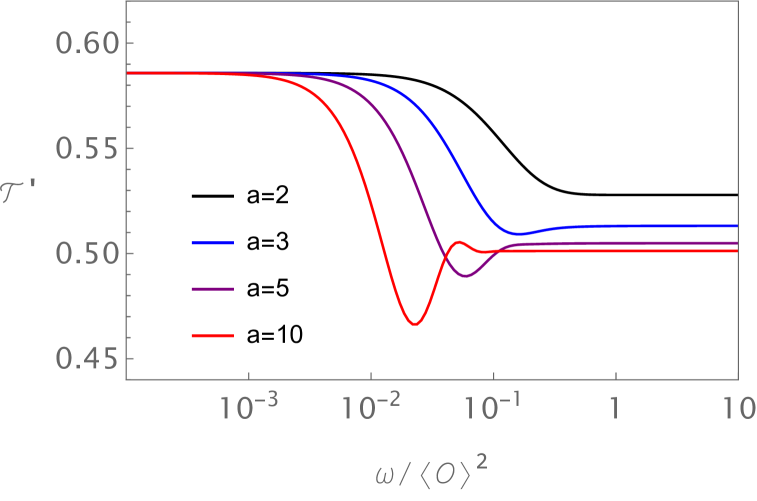
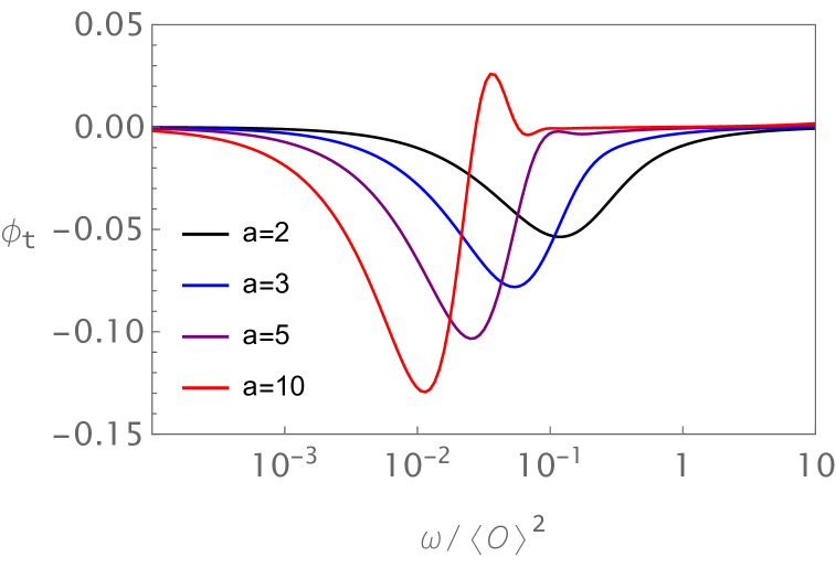
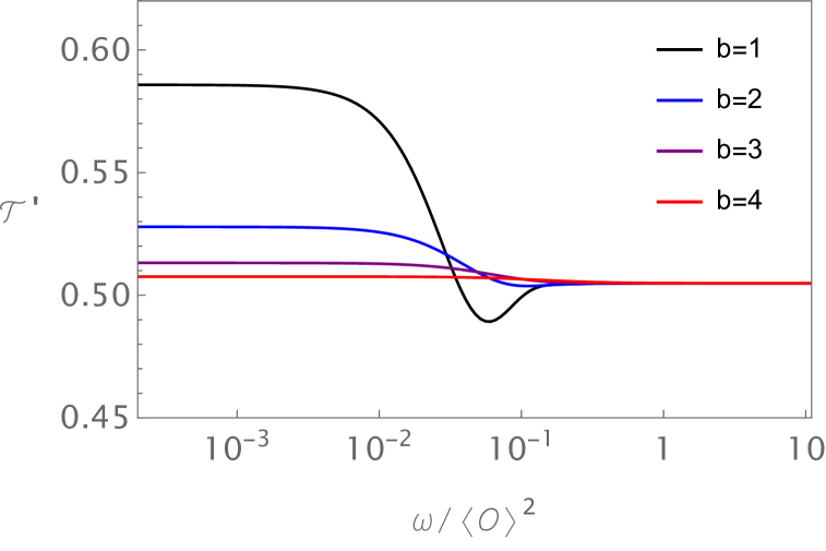
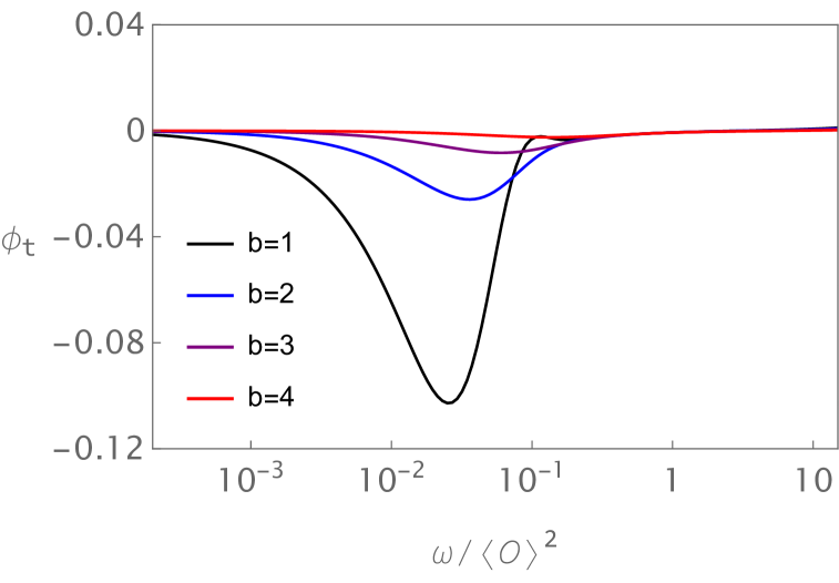
Figure 1: The plots of $\mathcal{T}^{\prime}$ and $\phi_{t}$ as functions of $\omega/\langle\mathcal{O}\rangle^{2}$ for varying $a$ with fixed $b=1$ (upper two plots), and varying $b$ with fixed $a=5$ (lower two plots).

In the following we consider the case $a>b$ and analyze the behaviors of the averaged transmission coefficient $\mathcal{T}^{\prime}$ defined in (2.18) and the phase shift of the transmission wave $\phi_{t}$ defined in (2.11). Fig. 1 illustrates the dependence of $\mathcal{T}^{\prime}$ and $\phi_{t}$ on $\omega/\mathcal{O}^{2}$ for different values of $a$ with $b=1$ in the upper two plots and for different values of $b$ with fixing $a=5$ in the lower two plots. From Fig. 1, we observe several key features of the transport coefficients. Unlike the conformal interface studied in (B.8), the transmission coefficient in this case is generally complex, and the averaged transmission coefficient $\mathcal{T}^{\prime}$ exhibits a dependence on the frequency $\omega$ of the incident wave. Furthermore, $\mathcal{T}^{\prime}$ and the phase $\phi_{t}$ approach constant values in both the low- and high-frequency limits of $\omega/\mathcal{O}^{2}$. In the low-frequency regime, the averaged transmission coefficient $\mathcal{T}^{\prime}$ converges to a constant that depends solely on the parameter $b$. This value coincides with the transmission coefficient for the brane profile $\psi(z)=bz$ of conformal interface. Simultaneously, the phase $\phi_{t}$ approaches zero, indicating that the transmission coefficient $\mathcal{T}$ is entirely governed by the IR region of the interface brane. Conversely, in the high-frequency regime, $\mathcal{T}^{\prime}$ approaches to a constant determined by the parameter $a$, matching the transmission coefficient for the brane profile $\psi(z)=az$ of the conformal interface. The phase $\phi_{t}$ also tends to zero in this limit, signifying that $\mathcal{T}$ is dominated by the UV region of the interface brane.

The UV and IR behaviour of the brane can be approximated by a straight line. Thus, the UV and IR limits of $\mathcal{T}^{\prime}$ always satisfy the bound proposed in [12]. The null energy condition requires $a\geq b$ ensuring that the UV value of $\mathcal{T}^{\prime}$ is never larger than its IR value. In the intermediate frequency region, $\mathcal{T}^{\prime}$ and $\phi_{t}$ may exhibit oscillatory behavior. As $a$ increases or $b$ decreases, the number of oscillations increases. Notably, in this intermediate frequency range, the averaged transmission coefficient $\mathcal{T}^{\prime}$ violates the lower bound proposed in [12].

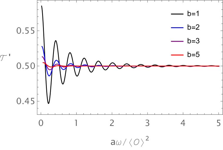
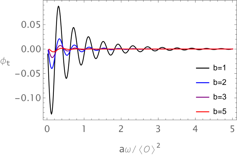
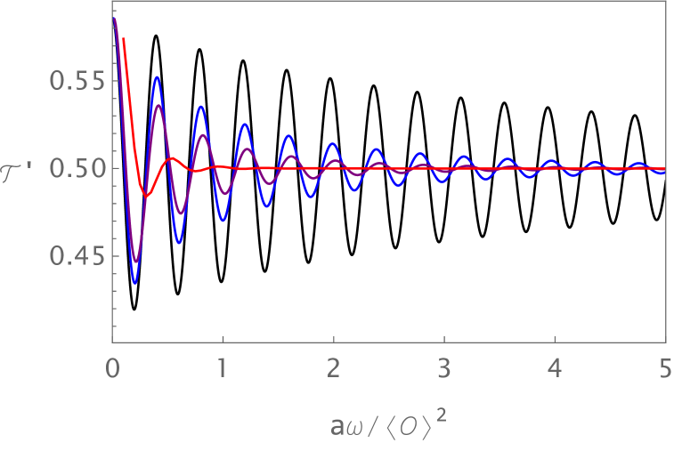
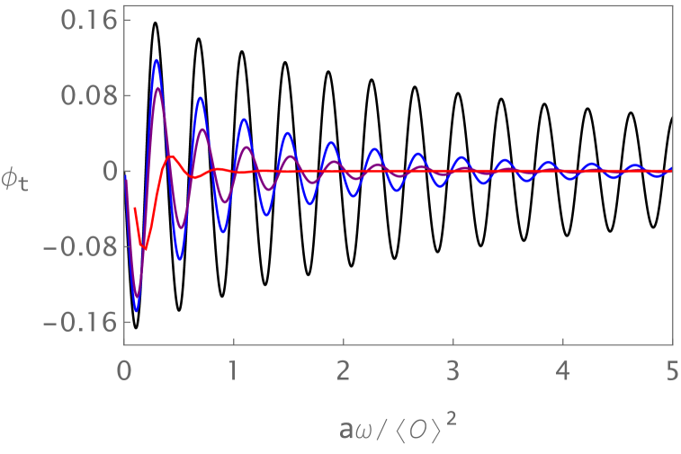
Figure 2: The plots of $\mathcal{T}^{\prime}$ and $\phi_{t}$ as functions of $a\omega/\langle\mathcal{O}\rangle^{2}$, for different values of $b$ with fixed $\omega/\langle\mathcal{O}\rangle^{2}=0.01$ (upper two plots) and for different values of $\omega/\langle\mathcal{O}\rangle^{2}$ with fixed $b=1$ (lower two plots). In the lower two plots, $\omega/\langle\mathcal{O}\rangle^{2}=0.001$ (black), $0.005$ (blue), $0.01$ (purple) and $0.05$ (red).

In Fig. 2, we show the plots of $\mathcal{T}^{\prime}$ and $\phi_{t}$ as functions of $a$. In the upper two plots, we fix the frequency and tune $b$. Both $\mathcal{T}^{\prime}$ and $\phi_{t}$ exhibit oscillations with a period of approximately $\omega a/\langle\mathcal{O}\rangle^{2}\simeq 0.4$. The amplitude of these oscillation decreases as the parameter $b$ is reduced or $\omega/\langle\mathcal{O}\rangle^{2}$ is increased.

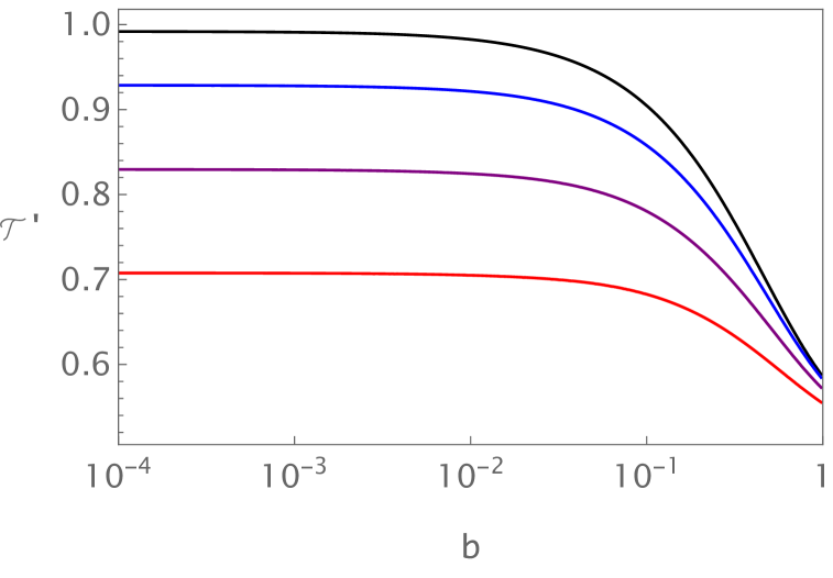
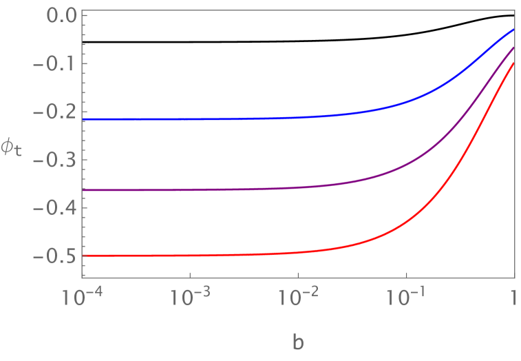
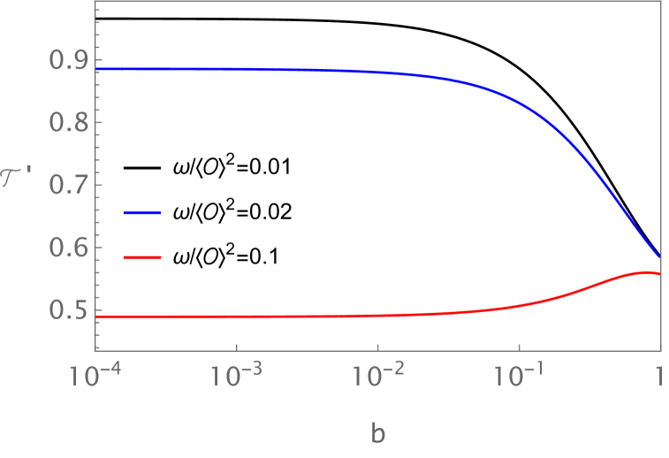
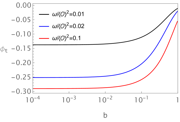
Figure 3: The plots of $\mathcal{T}^{\prime}$ and $\phi_{t}$ as functions of $b$, for different values of $a$ with fixed $\omega/\langle\mathcal{O}\rangle^{2}=0.01$ (upper two plots) and for different values of $\omega/\langle\mathcal{O}\rangle^{2}$ with fixed $a=2$ (lower two plots). In the upper two plots, $a=1$ (black), $3$ (blue), $5$ (purple), and $7$ (red).

In Fig. 3, we show the plots of $\mathcal{T}^{\prime}$ and $\phi_{t}$ as functions of $b$. Due to the null energy condition constraint $a\geq b$, we focus on the region where $b\in(0,1]$ with $a\geq 1$. We observe that, for the parameters considered, $\mathcal{T}^{\prime}$ and $\phi_{t}$ exhibit monotonic behavior for all values of $b$ within this region. This behavior contrasts with the trends observed in Fig. 2. Moreover, we find that when $b\to 0$, $\mathcal{T}^{\prime}$ approaches distinct values, which differs from its dependence on $a$. Furthermore, for a fixed value of $b$, we observe that $\mathcal{T}^{\prime}$ increases when $\omega/\langle\mathcal{O}\rangle^{2}$ decreases, and this is consistent with the observations in Fig. 1.

3.3 Two analytical examples

In this subsection we show two brane profiles for which analytical solution for the transmission coefficients can be derived. The induced metric for these two examples are asymptotically AdS₂ in the both UV and IR region. From the analytical solution, we observe the key features that were previously identified in the numerical example in Sec. 3.2.

3.3.1 The solution I with UV and IR asymptotically AdS₂

We consider the brane profile

$$\psi(z)=\frac{a}{b}\log(1+bz)\,.$$ (3.17)

The null energy condition requires that $ab>0$. Here we consider $a>0$ and $b>0$. The background brane geometry is asymptotically AdS with radius $L\sqrt{1+a^{2}}$ in the UV and radius $L$ in the IR. From the UV expansion, it exactly matches with (3.1) by identifying $A=a$ and $B=-ab/2$.

The profile for the scalar field is given by

$$\phi=\int_{0}^{z}ds\sqrt{\frac{abL}{s(1+bs)\sqrt{a^{2}+(1+bs)^{2}}}}\,,$$ (3.18)

and the potential is

$$V(\phi(z))=\frac{a(2+2a^{2}+5bz+3b^{2}z^{2})}{L(a^{2}+(1+bz)^{2})^{3/2}}\,.$$ (3.19)

In principle, this potential can be expressed as a function of $\phi$. The source of the scalar operator vanishes, and the VEV is $\langle\mathcal{O}\rangle=2\sqrt{abL}/(1+a^{2})^{1/4}$. We have $V_{\text{IR}}\to 0$ and $V_{\text{UV}}\to 2a/(L\sqrt{1+a^{2}})$.

The solution to the homogeneous part of ODE (2.22) takes the form

$$\begin{split}\xi_{l}(z)=&\,~c_{-}\,ze^{-i\sqrt{2}\omega z}(bz+1)^{\frac{ia\omega}{b}}\,U\left(\frac{1}{2}-\frac{i(\sqrt{2}-4a)\omega}{4b},~1+\frac{2ia\omega}{b},~\frac{2i\sqrt{2}(1+bz)\omega}{b}\right)\,\\ &+c_{+}\,ze^{-i\sqrt{2}\omega z}(bz+1)^{\frac{ia\omega}{b}}L\,\left(-\frac{1}{2}+\frac{i(\sqrt{2}-4a)\omega}{4b},~\frac{2ia\omega}{b},~\frac{2i\sqrt{2}(1+bz)\omega}{b}\right)\,,\end{split}$$ (3.20)

where $U(a,b,z)$ is the Tricomi confluent hypergeometric function, $L(a,b,z)$ is the generalized Laguerre polynomial and $c_{\pm}$ are constants. The infalling boundary condition at IR requires $c_{+}=0\,.$

From the solution (3.20) with $c_{+}=0$, matching the behavior of (3.11), we obtain the transmission coefficient

$$\mathcal{T}=1-\frac{ab}{C}\,U\left(\frac{1}{2}-\frac{i(\sqrt{2}-4a)\omega}{4b},~1+\frac{2ia\omega}{b},~\frac{2i\sqrt{2}\omega}{b}\right)\,,$$ (3.21)

where

$$\begin{split}C=&\,~\sqrt{2}b\,U\left(\frac{1}{2}-\frac{i(\sqrt{2}-4a)\omega}{4b},~1+\frac{2ia\omega}{b},~\frac{2i\sqrt{2}\omega}{b}\right)\\ &+\left(\sqrt{2}b+(2\sqrt{2}a-1)i\omega\right)U\left(\frac{3}{2}-\frac{i(\sqrt{2}-4a)\omega}{4b},~2+\frac{2ia\omega}{b},~\frac{2i\sqrt{2}\omega}{b}\right)\,\end{split}$$ (3.22)

and

$$\mathcal{R}=1-\mathcal{T}\,,~~~~~~c_{-}=\frac{2ab}{\omega^{2}C}\,.$$ (3.23)

Here we derive an analytic expression for the transport coefficients, which have a non-zero imaginary part and depend on $\omega$. Notably, $\mathcal{T}$ is determined by two parameters, $a$ and $\omega/b$. This is related to the fact that the IR behavior of the profile is special.

As $a\to 0$, the transmission coefficient approaches $\mathcal{T}=1$, corresponding to a brane straightly perpendicular to the boundary. When $a\to+\infty$, we find $\mathcal{T}=1/2$ for different values of $\omega/b$ by numerical computation. When $\omega/b\to 0$, due to the fact that

$$U\left(\frac{1}{2},\ 1,\ 2i\sqrt{2}\frac{\omega}{b}\right) \to-\frac{\gamma+\log\frac{i\omega}{\sqrt{2}b}}{\sqrt{\pi}}\,,~~~~\frac{\omega}{b}U\left(\frac{3}{2},\ 2,\ 2i\sqrt{2}\frac{\omega}{b}\right)\to-\frac{i}{\sqrt{2\pi}}\,,$$ (3.24)

where $\gamma$ is the Euler constant, and we have $\mathcal{T}\simeq 1+\mathcal{O}(\frac{\omega}{b}\log\frac{\omega}{b})\to 1$, consistent with $V_{\text{IR}}=0$. When $\omega/b\to\infty$, numerical results indicate $\mathcal{T}\to 1+a^{2}-a\sqrt{1+a^{2}}$. Additionally, $\mathcal{T}$ exhibit oscillatory behavior with $\omega$, and for certain value of $a$ and $\omega/b$, the real part of $\mathcal{T}$ can fall below the lower bound of $1/2$ proposed in [12]. These features align with those observed in the example discussed in Sec. 3.2.

3.3.2 The solution II with UV and IR asymptotically AdS₂

We consider another brane profile

$$\psi(z)=\frac{2a}{b}(\sqrt{1+bz}-1)\,.$$ (3.25)

The null energy condition requires $ab>0$ and we again assume $a>0$ and $b>0$. The background brane geometry is asymptotically AdS with radius $\sqrt{1+a^{2}}L$ in the UV and $L$ in the IR. From the UV expansion, it exactly matches (3.1) by identifying that $A=a,B=-ab/4$.

The profile for the scalar field is

$$\phi=\int_{0}^{z}ds\,\sqrt{\frac{abL}{2s(1+bs)\sqrt{1+a^{2}+bs}}}\,,$$ (3.26)

and the potential is

$$V(\phi(z))=\frac{a(4+4a^{2}+5bz)}{2L(1+a^{2}+bz)^{3/2}}\,.$$ (3.27)

The source of the scalar operator vanishes, and the VEV is $\langle\mathcal{O}\rangle=\sqrt{2abL}/(1+a^{2})^{1/4}$. We have $V_{\text{IR}}\to 0$ and $V_{\text{UV}}\to 2a/(L\sqrt{1+a^{2}})$.

The solution to the homogeneous part of ODE (2.22) takes the form

$$\begin{split}\xi_{l}(z)=&\,~c_{-}e^{-i\sqrt{\frac{3}{2}}\omega z}z\sqrt{1+bz}U\left(\frac{3}{4}+\frac{i(2a^{2}-1)\omega}{2\sqrt{6}b},\,\frac{3}{2},\,\frac{i\sqrt{6}(1+bz)\omega}{b}\right)\\ &+c_{+}e^{-i\sqrt{\frac{3}{2}}\omega z}z\sqrt{1+bz}L\left(-\frac{3}{4}-\frac{i(2a^{2}-1)\omega}{2\sqrt{6}b},\,\frac{1}{2},\,\frac{i\sqrt{6}(1+bz)\omega}{b}\right)\,,\end{split}$$ (3.28)

where $U(a,b,z)$ is the Tricomi confluent hypergeometric function, $L(a,b,z)$ is the generalized Laguerre polynomial and $c_{\pm}$ are constants. The infalling boundary condition at the IR requires $c_{+}=0\,.$

From the solution (3.28) with $c_{+}=0$, we obtain the transmission coefficient

$$\mathcal{T}=1+\frac{4iab\omega}{C_{2}}U\left(\frac{3}{4}+\frac{i(2a^{2}-1)\omega}{2\sqrt{6}b},~\frac{3}{2},~\frac{i\sqrt{6}\omega}{b}\right)\,,$$ (3.29)

where

$$\begin{split}C_{2}=&\,~2b\left[b-i(2a+\sqrt{6})\omega\right]U\left(\frac{3}{4}+\frac{i(2a^{2}-1)\omega}{2\sqrt{6}b},~\frac{3}{2},~\frac{i\sqrt{6}\omega}{b}\right)\\ &+(4a^{2}\omega-2\omega-3i\sqrt{6}b)\omega\,U\left(\frac{7}{4}+\frac{i(2a^{2}-1)\omega}{2\sqrt{6}b},~\frac{5}{2},~\frac{i\sqrt{6}\omega}{b}\right)\,,\end{split}$$ (3.30)

and

$$\mathcal{R}=1-\mathcal{T}\,,\ \ c_{-}=-\frac{8iab}{\omega C_{2}}\,.$$ (3.31)

Here, $\mathcal{T}$ is also determined by two parameters, $a$ and $\omega/b$, similar to the previous analytical example.

When $a\to 0$, we find that $\mathcal{T}=1+\mathcal{O}(a)$. When $a\to+\infty$, numerical computation show $\mathcal{T}=1/2$ for different $b,\omega$. When $\frac{\omega}{b}\to 0$, we can also find $\mathcal{T}\to 1$ and this rustlt is consistent with $V_{\text{IR}}=0$. When $\frac{\omega}{b}\to\infty$, we have $\mathcal{T}\to 1+a^{2}-a\sqrt{1+a^{2}}$ from numerical calculations. Oscillation behavior is also found for $\mathcal{T}$ in the intermediate frequency region with some parameters. And for certain value of $a$ and $\omega/b$, the real part of $\mathcal{T}$ can fall below the lower bound of $1/2$ proposed in [12] These properties again align with the key features discussed in earlier sections.

3.4 Another kind of UV asymptotically AdS geometry

From [21] it is known that when the brane is asymptotic AdS₂ in the UV limit, the profile $\psi(z)$ must satisfy $\psi(z)\to az^{n}$ with $n\geq 1$ as $z\to 0$. An interesting brane configuration is

$$\psi(z)=-az^{2}\,,$$ (3.32)

where the null energy condition requires that $a>0$. The induced metric of the brane is asymptotically AdS₂ in the UV and flat in the IR limit.

As noted in footnote 5, the source term in (2.22) vanishes. The exact solution to Eq. (2.22) is

$$\xi(z)=c_{-}\,ze^{-i\omega az^{2}}+c_{+}\,ze^{+i\omega az^{2}}\,,$$ (3.33)

where $c_{\pm}$ are two integral constants. The infalling boundary condition at IR requires

$$c_{+}=0\,.$$ (3.34)

Substituting the solution $\xi(z)=c_{-}ze^{-i\omega az^{2}}$ into equation (2.25), we find

$$\lambda(0)=-\frac{2i\,c_{-}}{\omega}\,.$$ (3.35)

The sourceless condition $\lambda(0)=0$ implies $c_{-}=0$, leading to

$$\xi(z)=0\,,$$ (3.36)

which indicates the perturbation in the $u_{\text{I,II}}$ directions vanishes.

From Eq. (2.23), the asymptotic behavior of $p(z)$ in the UV limit is

$$p(z)=p_{1}\,\sqrt{z}\log(z)\left(1+\mathcal{O}(z)\right)+p_{2}\,\sqrt{z}\left(1+\mathcal{O}(z)\right)\,,$$ (3.37)

where $p_{1}$ and $p_{2}$ are two integration constants. The sourceless condition for $p(z)$ requires $p_{1}=0$. Substituting $\xi(z)=0$ and the UV expansion of $p(z)$ with sourceless condition into Eqs. (2.26) and (2.27), we obtain

$$h_{\text{I}}(0)= -h_{\text{II}}(0)+\frac{1+\mathcal{R}-\mathcal{T}}{\omega^{2}a}\,,~~~~h_{\text{II}}(0)=\frac{2ia(\mathcal{R}+\mathcal{T}-1)+(1+\mathcal{R}-\mathcal{T})\,\omega}{2a\omega^{2}}\,.$$ (3.38)

Applying the sourceless conditions $h_{\text{I}}(0)=h_{\text{II}}(0)=0$, the transport coefficients are found to be

$$\mathcal{R}=0\,,\ \ \mathcal{T}=1\,.$$ (3.39)

Unlike the previous examples, the transmission coefficient is real and independent of the frequency of the injected waves. This result is identical to that of a topological interface, where the system is fully transmissive. Another similar result is obtained when the tension of the conformal brane vanishes [12]. It would be interesting to further explore other physical properties to understand the properties of this specific model.

More generally, as discussed in Section 3.1, one can consider a generic brane profile $\psi(z)$ with a UV expansion

$$\psi(z)=Az^{2}+Bz^{3}+\cdots\,,$$ (3.40)

where $A<0$. The solution to ODE (2.22) has a UV expansion of the form

$$\xi(z)=\xi_{1}z+\xi_{3}z^{3}+\frac{B(1+\mathcal{R}-\mathcal{T}+\omega^{2}\xi_{1}+2\xi_{3})}{2A}z^{4}+\mathcal{O}(z^{5})\,.$$ (3.41)

The scalar perturbation $p(z)$, dual to a scalar operator in ICFT, has the UV expansion

$$p(z)=p_{1}\sqrt{z}\log(z)\left(1+\mathcal{O}(z)\right)+p_{2}\sqrt{z}\left(1+\mathcal{O}(z)\right)\,,$$ (3.42)

where $p_{1}$ and $p_{2}$ are integration constants. Applying the sourceless condition $p_{1}=0$, the UV expansion of $p(z)$ simplifies to

$$p(z)=p_{2}\sqrt{z}\left(1+\mathcal{O}(z)\right)\,.$$ (3.43)

We first substitute $\psi(z),\xi(z)$ into Eq. (2.25), and find

$$\lambda(0)=-\frac{2i\xi_{1}}{\omega}\,.$$ (3.44)

The condition $\lambda(0)=0\,$ requires $\xi_{1}=0$. Second, substituting $\psi(z),\xi(z)$ into (2.27), we obtain

$$h_{\text{II}}(0)=-h_{\text{I}}(0)-\frac{1+\mathcal{R}-\mathcal{T}+2\xi_{3}}{A\omega^{2}}\,.$$ (3.45)

The sourceless conditions $h_{\text{II}}(0)=h_{\text{I}}(0)=0\,$ imply

$$1+\mathcal{R}-\mathcal{T}+2\xi_{3}=0\,.$$ (3.46)

Third, substituting $\psi(z),\xi(z),p(z)$ into (2.26), we find

$$h_{\text{I}}(0)=\frac{2iA\,(\mathcal{R}+\mathcal{T}-1)-(1+\mathcal{R}-\mathcal{T}+2\xi_{3})\omega}{2A\omega^{3}}\,.$$ (3.47)

The condition $h_{\text{I}}(0)=0\,$ requires

$$2iA\,(\mathcal{R}+\mathcal{T}-1)-(1+\mathcal{R}-\mathcal{T}+2\xi_{3})\,\omega=0\,.$$ (3.48)

Solving equations (3.48) and (3.46), we obtain

$$\mathcal{R}=-\xi_{3}\,,\ \ \mathcal{T}=1+\xi_{3}\,,$$ (3.49)

which satisfy the relation

$$\mathcal{R}+\mathcal{T}=1\,.$$ (3.50)

For the specific case $\psi(z)=-az^{2}$, the exact solution for $\xi(z)$ exists. The infalling boundary condition and $\xi_{1}=0$ imply $\xi_{3}=0$, leading to $\mathcal{R}=0,\mathcal{T}=1$.

4 Conclusions and open questions

We have studied the properties of energy transport in a $1+1$-dimensional ICFT system with a non-conformal interface using holographic duality. Our focus has been on systems where the central charges of the left and right CFTs are identical, and the interface hosts a localized scalar operator. In the holographic framework, the system is described by a left and right bulk gravity joined along a brane anchored at the interface, with a dynamical scalar field localized on the brane.

By imposing sourceless boundary conditions for the fluctuations on the interface brane, or equivalently enforcing the energy conservation at the interface in the dual theory, we consistently observe that the sum of transmission and reflection coefficients satisfies $\mathcal{R}+\mathcal{T}=1$. Furthermore, the transmission coefficient $\mathcal{T}$ is generally complex. We interpret the real parts of these coefficients as the averaged transmission and reflection coefficients, and analyze their behavior across several brane profile configurations. Through one numerical and two analytical examples, we demonstrate that, in addition to the complex nature of the coefficients, the energy transports depend on the frequency of the injected wave, in contrast to conformal interfaces, where these energy transport coefficients remain real constants independent of frequency. Notably, for cases where the induced metric on the interface brane interpolates between two AdS₂ geometries, the averaged transmission coefficient transitions from the UV conformal interface value at high frequencies to the IR conformal interface value at low frequencies. In the intermediate frequency regime, the coefficient may oscillate as a function of frequency and can violate the bound found in [12]. Additionally, in Sec. 3.4 we find a nontrivial example exhibiting complete transmissivity, which shares similarities with the behavior of a topological interface.

Several open questions remain for future exploration. A natural extension of this work would be to generalize our study to cases where the left and right CFTs have different central charges. Such scenarios are expected to involve more complicated numerics. One could also employ the non-perturbative methods [13], such as studying the system at finite temperature, to investigate the brane profile and energy fluxes in detail. Another interesting direction is to explore the real-time evolution of the system. One could excite a localized energy flux on the left CFT and observe the system’s dynamics, thereby elucidating the role of the complex and frequency-dependent energy transport properties. Finally, it would be valuable to study energy transport directly from the field theory perspective. While non-conformal interfaces in field theory have been explored in works such as [26], the properties of energy transport in these systems warrant further investigation. We hope to address some of these questions in future work.

Acknowledgments

We thank Shan-Ming Ruan and Ya-Wen Sun for useful discussions. This work is supported by the National Natural Science Foundation of China grant No. 12375041.

Appendix A The useful equations

In this appendix we show additional equations that were not included in the main text but are essential for the analysis.

A.1 Equations of the system

We begin by writing out the equations of motion for the fields in the system. These equations are fundamental for solving both the background configuration and the fluctuations of the system.

The continuous condition for the metric on $Q$ is given by

$$g_{ab}\frac{\partial x_{\text{I}}^{a}}{\partial y^{\mu}}\frac{\partial x_{\text{I}}^{b}}{\partial y^{\nu}}\bigg{|}_{\text{I}}=g_{ab}\frac{\partial x_{\text{II}}^{a}}{\partial y^{\mu}}\frac{\partial x_{\text{II}}^{b}}{\partial y^{\nu}}\bigg{|}_{\text{II}}\,.$$ (A.1)

The equations of motion are

$$R^{\text{I}}_{ab}-\frac{1}{2}g^{\text{I}}_{ab}R^{\text{I}}-\frac{1}{L^{2}}g^{\text{I}}_{ab} = 0\,,$$ (A.2)

$$R^{\text{II}}_{ab}-\frac{1}{2}g^{\text{II}}_{ab}R^{\text{II}}-\frac{1}{L^{2}}g^{\text{II}}_{ab} = 0\,,$$ (A.3)

$$\Delta K_{\mu\nu}-h_{\mu\nu}\Delta K+\left[(\partial\phi)^{2}+V(\phi)\right]h_{\mu\nu}-2\partial_{\mu}\phi\partial_{\nu}\phi = 0\,,$$ (A.4)

$$2\partial_{\mu}(\sqrt{-h}h^{\mu\nu}\partial_{\nu}\phi)-\sqrt{-h}\frac{dV(\phi)}{d\phi} = 0\,,$$ (A.5)

where $\Delta X\equiv X_{\text{I}}-X_{\text{II}}$ with $X$ as $K_{\mu\nu}$ or $K$. Equations (A.2) and (A.3) describe the metric fields in the left half and the right bulk regions, respectively, while (A.4) and (A.5) are the equations on the interface brane $Q$. Sepcifically, (A.1) and (A.4) are the generalized Isreal junction conditions.

A.2 Equations for the fluctuations

In Sec. 2.1.1, we have written out the equations of motion for $\xi(z)$ and $p(z)$. The coefficients $c_{1},c_{2},c_{3}$ in Eq. (2.23) are

$$\begin{split}c_{1}&=\frac{1}{4}\left[\frac{1}{z^{2}}+4\omega^{2}(1+\psi^{\prime 2})+\frac{4\psi^{\prime}\psi^{\prime\prime}}{z(\psi^{\prime 2}+1)}+\frac{(2-5\psi^{\prime 2})\psi^{\prime\prime 2}}{(\psi^{\prime 2}+1)^{2}}+\frac{6\psi^{\prime}\psi^{(3)}}{\psi^{\prime 2}+1}+\frac{(\psi^{(3)})^{2}}{\psi^{\prime\prime 2}}-\frac{2(z\psi^{(4)}+\psi^{(3)})}{z\psi^{\prime\prime}}\right]\,,\\ c_{2}&=-\frac{z\psi^{(3)}\psi^{\prime}(\psi^{\prime 2}+1)+(\psi^{\prime 2}+1)\psi^{\prime\prime}(\psi^{\prime}-i\omega z)+z(1-\psi^{\prime 2})\psi^{\prime\prime 2}}{2\omega\sqrt{z}(\psi^{\prime 2}+1)^{5/4}\sqrt{-L\psi^{\prime\prime}}}\,,\\ c_{3}&=\frac{z\psi^{(3)}\psi^{\prime}(\psi^{\prime 2}+1)+(\psi^{\prime 2}+1)\psi^{\prime\prime}(\psi^{\prime}+i\omega z)+z(1-\psi^{\prime 2})\psi^{\prime\prime 2}}{2\omega\sqrt{z}(\psi^{\prime 2}+1)^{5/4}\sqrt{-L\psi^{\prime\prime}}}\,.\end{split}$$ (A.6)

Below, we provide the detailed form of three equations of $\lambda(z),h_{\text{I}}(z),h_{\text{II}}(z)$,

$$\begin{split}\lambda=&\,~\frac{(\bm{I}+\bm{R}-\bm{T})z^{3}+2\xi}{i\omega z}\,,\\ h_{\text{I}}=&\,~\frac{(1-\omega^{2}z^{2})\xi-z\xi^{\prime}}{\omega^{2}\psi^{\prime}z^{2}}+\sqrt{\frac{-Lz}{\psi^{\prime\prime}}}\frac{(1+\psi^{\prime 2})\left(\psi^{\prime\prime}+z\psi^{(3)}\right)-z\psi^{\prime}\psi^{\prime\prime}}{\omega^{2}(1+\psi^{\prime 2})^{7/4}z}p\,\\ &+\frac{2\sqrt{-Lz\psi^{\prime\prime}}}{\omega^{2}(1+\psi^{\prime 2})^{3/4}}p^{\prime}+\frac{1}{\omega^{3}\psi^{\prime}(1+\psi^{\prime 2})}\cdot\text{\bf s}\,,\\ h_{\text{II}}=&\,-h_{\text{I}}+\frac{2(1-\omega^{2}z^{2})\xi-2z\xi^{\prime}}{\omega^{2}\psi^{\prime}z^{2}}-\frac{z\left[2(\bm{I}+\bm{R}-\bm{T})+i(\bm{I}-\bm{R}+\bm{T})\omega\psi^{\prime}z\right]}{\omega^{2}\psi^{\prime}}\,,\end{split}$$ (A.7)

where

$$\begin{split}\text{\bf s}=&\left[(\bm{T}-\bm{R})\omega z-\bm{I}\right]+i\left[\bm{T}+(\bm{R}-\bm{I})(1+\omega^{2}z^{2})\right]\psi^{\prime}(1+\psi^{\prime 2})\\ &+(\bm{I}+\bm{R}+\bm{T})\omega\psi^{\prime 4}z+\left[2\omega\bm{T}+i(\bm{R}+\bm{T}-\bm{I})\psi^{\prime\prime}\right]\psi^{\prime 2}z\,.\end{split}$$ (A.8)

A.3 Equations for the boundary conditions

In this appendix we show the IR boundary condition for the scalar field in Sec. 3.2. From (2.23), the asymptotic behavior of $p(z)$ in IR limit is

$$\begin{split}p(z)=&\,~p_{0}e^{-i\omega\sqrt{1+b^{2}}z}\left(1-\frac{i(1-ab\omega^{2}+b^{2}\omega^{2})}{\sqrt{1+b^{2}}\omega z}+\mathcal{O}(z^{-2})\right)\\ &+e^{+i\omega bz}\left(\frac{e^{i(a-b)\omega}\sqrt{a-b}\,(\mathcal{R}+\mathcal{T})}{\sqrt{2L}\omega^{2}(1+b^{2})^{1/4}z}+\mathcal{O}(z^{-2})\right)\\ &+e^{-i\omega bz}\left(\frac{e^{-i(a-b)\omega}\sqrt{a-b}}{\sqrt{2L}\omega^{2}(1+b^{2})^{1/4}z}+\mathcal{O}(z^{-2})\right)\,,\end{split}$$ (A.9)

where $p_{0}$ is an integration constant which can be determined by the sourceless boundary condition. We have dropped the out-going wave $e^{+i\omega\sqrt{1+b^{2}}z}$.

Appendix B Briefly review of the transport in conformal interface

In this appendix, we show that the gauge choice considered in Sec. 2.1.1 allows us to consistently reproduce the results for energy transports in conformal interface [12].

The bulk equation is solved by the planar AdS₃ solution

$$ds^{2}_{A}=\frac{L^{2}_{A}}{u^{2}_{A}}\bigg{[}-dt^{2}_{A}+dx^{2}_{A}+du^{2}_{A}\bigg{]}\,,~~~A=\text{I\,,~~II}\,.$$ (B.1)

The interface brane is described by

$$x_{\text{I}}=u_{\text{I}}\tan\alpha,\ \ x_{\text{II}}=-u_{\text{II}}\tan\beta.$$ (B.2)

The junction condition gives

$$\nu\equiv\frac{L_{\text{II}}}{L_{\text{I}}}=\frac{\cos\beta}{\cos\alpha}\,,~~~~\sigma=\frac{\sin(\alpha+\beta)\sec\beta}{L_{\text{I}}}\,,$$ (B.3)

where $\sigma$ is the brane tension. These two equations determine the value of $\alpha$ and $\beta$.

Since the study in the main text focuses on the case $\nu=1$, we generalize the fluctuations to arbitrary $\nu$. The first order perturbation of the bulk metric is given by

$$\begin{split}[ds^{2}]_{\text{I}}=&4GL_{\text{I}}\epsilon\left[e^{i\omega(t_{\text{I}}-x_{\text{I}})}(dt_{\text{I}}-dx_{\text{I}})^{2}+\mathcal{R}e^{i\omega(t_{\text{I}}+x_{\text{I}})}(dt_{\text{I}}+dx_{\text{I}})^{2}\right]\,,\\ [ds^{2}]_{\text{II}}=&4GL_{\text{I}}\nu\,\epsilon\mathcal{T}e^{i\omega(t_{\text{II}}-x_{\text{II}})}(dt_{\text{II}}-dx_{\text{II}})^{2}\,,\end{split}$$ (B.4)

where $\mathcal{R}$ and $\mathcal{T}$ are the reflection and transmission coefficients, respectively, and $\epsilon$ is the injected energy flux. The perturbed brane is described by

$$\begin{split}t_{\text{I}}=&\,~t+\frac{G\epsilon}{L_{\text{I}}}e^{i\omega\tau}\lambda(z)\,,\ x_{\text{I}}=z\tan\alpha+\frac{2G\epsilon}{L_{\text{I}}}e^{i\omega\tau}h_{\text{I}}(z)\,,\ u_{\text{I}}=z+\frac{2G\epsilon}{L_{\text{I}}}e^{i\omega\tau}\xi(z)\,,\\ t_{\text{II}}=&\,~t-\frac{G\epsilon}{L_{\text{I}}}e^{i\omega\tau}\lambda(z)\,,\ x_{\text{II}}=-z\nu\tan\beta+\frac{2G\epsilon}{L_{\text{I}}}e^{i\omega\tau}h_{\text{II}}(z)\,,\ u_{\text{II}}=\nu z-\frac{2G\epsilon}{L_{\text{I}}}e^{i\omega\tau}\xi(z)\,,\end{split}$$ (B.5)

where $t$ and $z$ are the intrinsic coordinates of the brane.

Defining

$$\delta(z)\equiv\sin\alpha\,\csc\beta\,h_{\text{I}}(z)+h_{\text{II}}(z)\,,$$ (B.6)

the perturbed equation of motion reduce to a system of four first-order differential equations for fields $\lambda(z),\ \xi(z),\ h_{\text{I}}(z),\ \delta(z)$. To solve this system, we impose the sourceless boundary conditions at $z=0$ [12]

$$\lambda(0)=0,\ \xi(0)=0,\ h_{\text{I}}(0)=0,\ \delta(0)=0\,,$$ (B.7)

ensuring that the intersection point between the brane and the boundary remains fixed. Notably, $\xi(0)=0$ is automatically satisfied. Additionally, we impose “no out-going wave” condition, which eliminates out-going wave $e^{i\omega(t+\sec\alpha\,z)}$. With these boundary conditions, we can fix the four functions and the transports $\mathcal{R},\mathcal{T}$ are uniquely determined. From the solution, we obtain the holographic energy transport coefficients

$$\mathcal{T}=\frac{2\cos\beta}{\cos\beta(1+\sin\alpha)+\cos\alpha(1+\sin\beta)}\,,~~~~\mathcal{R}=1-\mathcal{T}\,.$$ (B.8)

For the case $L_{\text{I}}=L_{\text{II}}$, the transmission coefficient $\mathcal{T}$ lies in the interval $[\frac{1}{2},1]$. The brane configuration corresponding to $\mathcal{T}=1$ is given by $x_{\text{I}}=x_{\text{II}}=0$, while the brane configuration for $\mathcal{T}=\frac{1}{2}$ coincides with the AdS boundary at $z=0$.

References

- [1] I. Affleck and A. W. W. Ludwig, Universal noninteger ‘ground state degeneracy’ in critical quantum systems, Phys. Rev. Lett. 67 (1991), 161-164.
- [2] K. Sakai and Y. Satoh, Entanglement through conformal interfaces, JHEP 12 (2008), 001 [arXiv:0809.4548].
- [3] T. Quella, I. Runkel and G. M. T. Watts, Reflection and transmission for conformal defects, JHEP 04 (2007), 095 [arXiv:hep-th/0611296].
- [4] M. Meineri, J. Penedones and A. Rousset, Colliders and conformal interfaces, JHEP 02 (2020), 138 [arXiv:1904.10974].
- [5] A. Karch, Y. Kusuki, H. Ooguri, H. Y. Sun and M. Wang, Universal Bound on Effective Central Charge and Its Saturation, Phys. Rev. Lett. 133 (2024) no.9, 091604 [arXiv:2404.01515].
- [6] M. Oshikawa and I. Affleck, Defect lines in the Ising model and boundary states on orbifolds, Phys. Rev. Lett. 77 (1996), 2604-2607 [arXiv:hep-th/9606177].
- [7] I.V. Lerner, V. I. Yudson and I. V. Yurkevich, Quantum Wire Hybridized With a Single- Level Impurity, Phys. Rev. Lett. 100, 256805 (2008) arXiv:0711.4919.
- [8] C. Rylands and N. Andrei, Quantum impurity in a Luttinger liquid: Exact solution of the Kane-Fisher model, Phys. Rev. B 94 (2016), 115142 [arXiv:1606.07472].
- [9] M. Billò, V. Gonçalves, E. Lauria and M. Meineri, Defects in conformal field theory, JHEP 04 (2016), 091 [arXiv:1601.02883].
- [10] J. Zaanen, Y. W. Sun, Y. Liu and K. Schalm, Holographic Duality in Condensed Matter Physics, Cambridge Univ. Press (2015).
- [11] S. A. Hartnoll, A. Lucas and S. Sachdev, Holographic quantum matter, MIT Press.
- [12] C. Bachas, S. Chapman, D. Ge and G. Policastro, Energy Reflection and Transmission at 2D Holographic Interfaces, Phys. Rev. Lett. 125 (2020) no.23, 231602 [arXiv:2006.11333].
- [13] C. Bachas, Z. Chen and V. Papadopoulos, Steady states of holographic interfaces, JHEP 11 (2021), 095 [arXiv:2107.00965].
- [14] S. A. Baig and A. Karch, Double brane holographic model dual to 2d ICFTs, JHEP 10 (2022), 022 [arXiv:2206.01752].
- [15] C. Bachas, S. Baiguera, S. Chapman, G. Policastro and T. Schwartzman, Energy Transport for Thick Holographic Branes, Phys. Rev. Lett. 131 (2023) no.2, 021601 [arXiv:2212.14058].
- [16] I. Brunner and C. Schmidt-Colinet, Reflection and transmission of conformal perturbation defects, J. Phys. A 49 (2016) no.19, 195401 [arXiv:1508.04350].
- [17] S. A. Baig and S. Shashi, Transport across interfaces in symmetric orbifolds, JHEP 10 (2023), 168 [arXiv:2301.13198].
- [18] P. Biswas, S. Das and A. Dinda, Moving interfaces and two-dimensional black holes, JHEP 05 (2024), 329 [arXiv:2401.11451].
- [19] S. A. Baig, A. Karch and M. Wang, Transmission coefficient of super-Janus solution, JHEP 10 (2024), 235 [arXiv:2408.00059].
- [20] M. Gutperle and C. Hultgreen-Mena, Janus and RG-interfaces in minimal 3d gauged supergravity, [arXiv:2412.16749].
- [21] Y. Liu, H. D. Lyu and C. Y. Wang, On AdS3/ICFT2 with a dynamical scalar field located on the brane, JHEP 10 (2024), 001 [arXiv:2403.20102].
- [22] H. Kanda, M. Sato, Y. k. Suzuki, T. Takayanagi and Z. Wei, AdS/BCFT with brane-localized scalar field, JHEP 03 (2023), 105 [arXiv:2302.03895].
- [23] A. Banerjee, A. Mukhopadhyay and G. Policastro, Nambu-Goto equation from three-dimensional gravity, JHEP 09 (2024), 013 [arXiv:2404.02149].
- [24] J. Erdmenger, M. Flory and M. N. Newrzella, Bending branes for DCFT in two dimensions, JHEP 01 (2015), 058 [arXiv:1410.7811].
- [25] J. Erdmenger, M. Flory, C. Hoyos, M. N. Newrzella, A. O’Bannon and J. Wu, Holographic impurities and Kondo effect, Fortsch. Phys. 64 (2016), 322-329 [arXiv:1511.09362].
- [26] S. Kim, P. Kraus and Z. Sun, Codimension one defects in free scalar field theory, [arXiv:2502.19547].