Including local feature interactions in deep non-negative matrix factorization networks improves performance.
Abstract
The brain uses positive signals as a means of signaling. Forward interactions in the early visual cortex are also positive, realized by excitatory synapses. Only local interactions also include inhibition. Non-negative matrix factorization (NMF) captures the biological constraint of positive long-range interactions and can be implemented with stochastic spikes. While NMF can serve as an abstract formalization of early neural processing in the visual system, the performance of deep convolutional networks with NMF modules does not match that of CNNs of similar size. However, when the local NMF modules are each followed by a module that mixes the NMF’s positive activities, the performances on the benchmark data exceed that of vanilla deep convolutional networks of similar size. This setting can be considered a biologically more plausible emulation of the processing in cortical (hyper-)columns with the potential to improve the performance of deep networks.
keywords:
deep neuronal networks , non-negative matrix factorization (NMF) , backpropagation error learning[label1]organization=University of Bremen, addressline=Institute for Theoretical Physics, city=Bremen, postcode=28359, state=Bremen, country=Germany
[label2]organization=University of Bremen, addressline=Institute of Electrodynamics and Microelectronics (ITEM.ids), city=Bremen, postcode=28359, state=Bremen, country=Germany
1 Introduction
The success of modern neural networks has often come from incorporating principles inspired by their biological role model: the brain. A well-known example is the introduction of convolutional layers (Lecun et al., 1998a), which mirror the organization of the visual cortex in biological brains. Neurons in the visual cortex have localized receptive fields, meaning they respond stereotypically to stimuli in specific regions of the visual field (Hubel and Wiesel, 1962). This principle first adopted by (Fukushima, 1980), now enables convolutional neural networks (CNNs) to efficiently detect patterns and hierarchies in images. This biologically inspired design has been crucial in advancing the performance of machine learning models in computer vision (Lecun et al., 1998b).
Despite the success of incorporating some biological principles, several key constraints in biological neural systems remain under-explored in machine learning. For example, Dale’s Law, one of the core principles of neurobiology, dictates that neurons are either excitatory or inhibitory but not both (Strata and Harvey, 1999).
Another often overlooked biological aspect is the nature of long-range connections between cortical areas, such as those between the primary visual cortex (V1) and higher visual areas. In biological neural systems, long-range connections are predominantly excitatory, in contradiction with usual deep CNNs. In the cortex, the excitatory postsynaptic currents (EPSCs) are also received by inhibitory neurons, which in turn locally modulate pyramidal (Pyr) cells through inhibitory postsynaptic currents (IPSCs) (Yang et al., 2013), typically in a different layer. This configuration implies that while interactions of both signs are essential for modulating neural responses and shaping information processing locally, the primary flow of information across layers and areas is governed by excitatory or ”positive” connections.
Our work also builds on the hypothesis that receptive fields in the visual cortex develop through sparse coding mechanisms—where neural activity is distributed such that only a small subset of neurons responds to a given stimulus (Olshausen and Field, 2006). Non-negative matrix factorization (NMF) (Lee and Seung, 1999) (Lee and Seung, 2000) provides an elegant mathematical framework that simultaneously satisfies two key biological constraints: the positivity of long-range neural interactions and the tendency toward sparse representations. For instance, (Hoyer, 2003) demonstrated that such sparse coding mechanisms could be effectively modeled using NMF. By imposing both non-negativity and sparseness constraints, this work showed that NMF can learn parts-based, interpretable representations similar to the mechanism yielding receptive fields first proposed in (Olshausen and Field, 1996).
While Non-negative Matrix Factorization (NMF) is a powerful unsupervised learning technique used in various fields, including signal processing, computer vision, and data mining (Lee and Seung, 1999), applying it effectively to supervised tasks like computer vision presents significant challenges. When used in isolation, NMF typically cannot match the performance of modern deep learning architectures such as CNNs. Previous works have attempted to bridge this gap by combining NMF with deep learning approaches.
For instance, (Geng et al., 2021) proposed using an NMF layer on top of a convolutional model. However, such implementations often reinitialize and retrain the NMF components from scratch after each forward pass, leading to computational inefficiency and potential instability. In contrast, our approach implements a hierarchical NMF architecture where the NMF weights are treated as learnable parameters and optimized through back-propagation alongside the network’s other parameters. This enables the NMF components to adapt continuously to the task requirements while maintaining their biological constraints.
Missing in current networks using NMF are local interactions that include inhibition, an important property of cortical microcircuits. After briefly reviewing NMF, we introduce a convolutional network architecture where we exchange CNN modules with NMF modules. We then propose a simple but novel extension of the NMF network where subsequent 1x1 convolutional layers are inserted. Thereby, we realize general local interactions among the features of the NMF modules in analogy to cortical hyper-columns, which makes these networks a step toward more biologically realistic models. When optimized with back-propagation (both the 1x1 CNNs and the NMF modules), we show that these networks exhibit performances on benchmark data sets that can exceed the values of pure CNNs with the same architecture.
2 Methods
2.1 Non-negative Matrix Factorization (NMF)
Non-negative Matrix Factorization (NMF) (Lee and Seung, 1999) (Lee and Seung, 2000) is a technique used to decompose a non-negative matrix of input vectors into two lower-dimensional non-negative matrices and , such that , where , , and . The goal is to minimize the difference between and the product while ensuring that both and remain non-negative. It is often expressed as:
| (1) |
minimizing the Kullback-Leibler divergence defined as:
| (2) |
leads to the following multiplicative update rules for and (Lee and Seung, 2000):
| (3) |
| (4) |
| (5) |
2.2 Deep Non-negative Matrix Factorization in a Neural Network
In this work, we extend NMF to a deep learning setting (Chen et al., 2022) by integrating it into a network architecture. Specifically, we treat the factorized matrices and as components of a neural network layer. The matrix is used as the weight matrix of the layer, while the matrix represents the activation values (neuron outputs) of the layer.
The challenge lies in adapting the unsupervised nature of NMF (Lee and Seung, 1999) for use in a multi-layer supervised context, such as classification, where the learned weights must optimize a specific task-related objective function (Ciampiconi et al., 2023) (Tian et al., 2022). In classical NMF, both and are updated iteratively using multiplicative update rules, following the Expectation-Maximization algorithm, to minimize the factorization error. However, when applying NMF within a neural network, directly updating in an unsupervised manner could lead to weights that are not aligned with the task objective (e.g., classification loss). To address this, we decouple the update process for from the factorization step.
Instead of updating using the NMF update rules, we keep fixed during the forward pass, using it to calculate the activations for each layer. The neuron values at each iteration, on the other hand, follow a similar approach to the NMF update rule. For one pattern the general update rule for in a hidden layer at each iteration is formulated as:
| (6) |
Where denotes the input and is the weight matrix. Unless said otherwise, is set to 1, which leads to an equation similar to 3. During each forward pass at each layer, we first initialize values to , where is the number of neurons, and we repeat the update rule (6) for times until getting the output values of the layer.
2.3 Approximated back-propagation
A significant practical challenge in implementing NMF-based neural architectures is the computational overhead of back-propagation through iterative steps. Conventional NMF requires iterations ( usually ranging from 20 to 100 iterations) in the forward pass, and automatic differentiation frameworks like PyTorch must store gradients for each iteration to compute the backward pass accurately. This creates substantial memory requirements and computational bottlenecks, especially for deep networks or large-scale applications.
We address this limitation by using an efficient approximation to the back-propagation procedure that requires only a single step, eliminating the need to save and back-propagate through all intermediate iterations performed during the forward pass. This method introduced in (Rotermund and Pawelzik, 2019) dramatically reduces both memory consumption and computation time while maintaining comparable accuracy to full back-propagation through all iterations. For convenience we here only sketch the basic idea underlying this approach but refer to (Rotermund and Pawelzik, 2019) for the detailed derivations. Back-propagation requires the partial derivatives and . These derivatives can be obtained from the the h-dynamics for a single pattern :
| (7) | |||||
| (8) |
where . If we would change we would obtain a deterministic change of the output in one step of this dynamics:
| (9) | |||||
| (10) | |||||
| (11) |
That is, we now have the changes of the original depending on changes of the input :
| (12) |
This formula preserves normalization of since .
By comparing with the total differential, we obtain
| (13) |
Following the same logic we have
| (14) | |||
| (15) | |||
| (16) |
which (again via the total differential) leads to
| (17) |
These derivatives are then used to change the weights according to
| (18) |
where
| (19) |
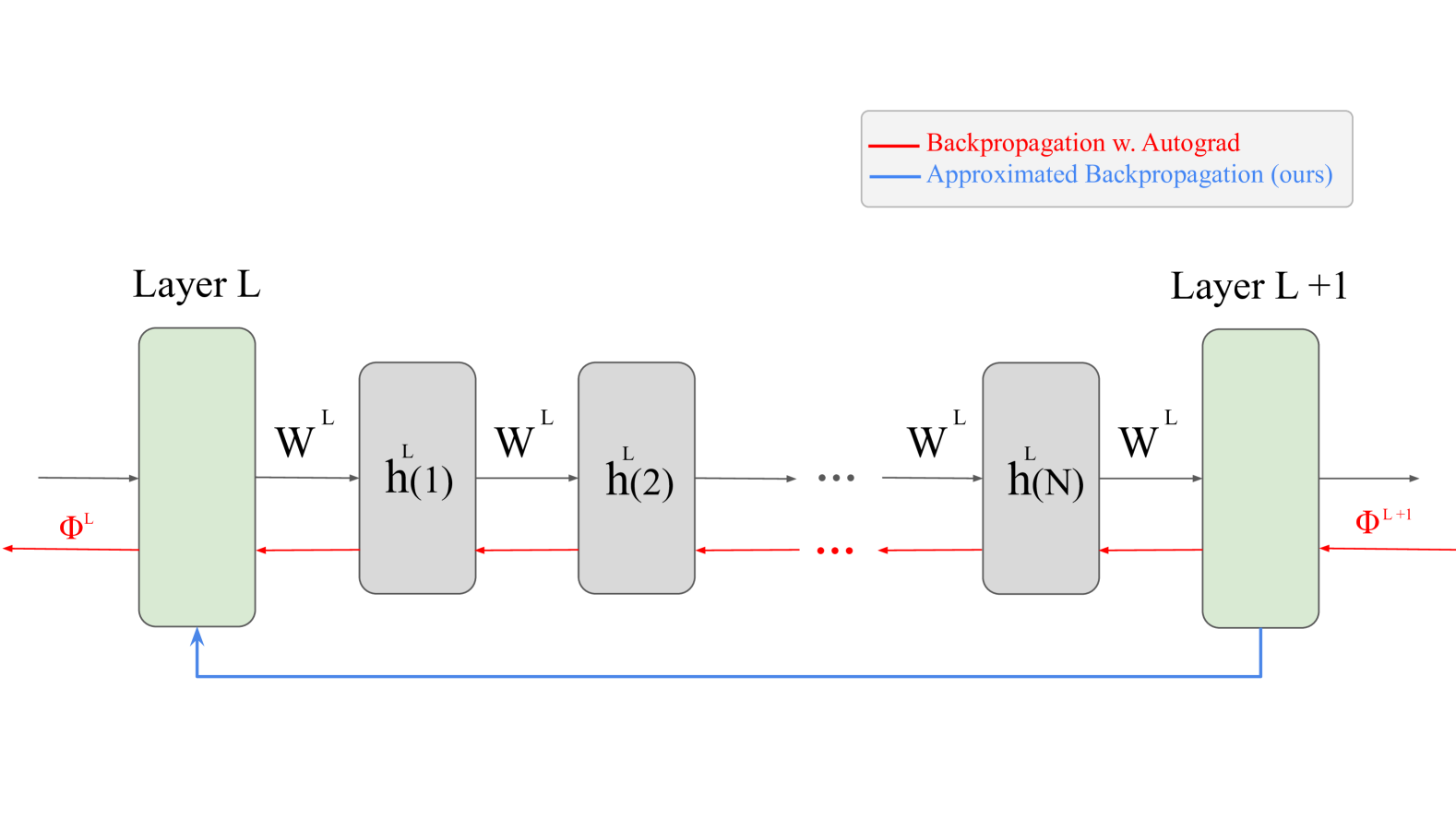
is the back-propagated error . This method is applied only to the final states . Figure 2 illustrates how this approach reduces the amount of computations.
2.3.1 Updating the Weight Matrix
To make the weight matrix more suitable for classification, we update through back-propagation using an optimizer (e.g., Adam). This ensures that is optimized based on the task’s objective function rather than simply minimizing the reconstruction error from NMF. However, a challenge arises as gradient-based updates do not inherently preserve the non-negativity and normalization properties of . Since NMF requires that remains non-negative and normalized, we cannot directly update with the raw gradient values. Instead, we introduce a trainable auxiliary matrix , which has the same dimensions as , and at each network update, the optimizer will update using the error calculated in the equation 18. Based on this parameter, during each forward pass, the weight is obtained based on:
| (20) |
which applies two main transformations:
-
1.
Non-negativity constraint: We enforce non-negativity by setting , where represents the element-wise absolute value of .
-
2.
Normalization: We normalize each row of to ensure the sum of each row is equal to 1, ensuring that remains a valid factorization matrix.
The transformation ensures that the weight matrix retains the necessary properties for NMF while still being adaptable for learning tasks.
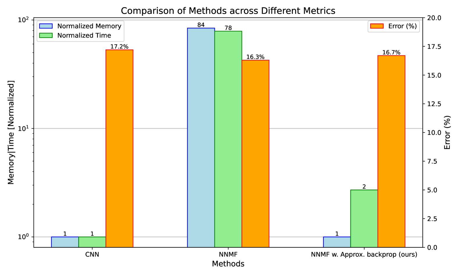
Our empirical evaluation confirms the computational efficiency of the proposed approximate back-propagation (BP) method while maintaining performance. Figure 1 compares three architectures: a normal convolutional network, an NMF-based network with full BP via Torch Autograd, and our NMF network with approximate BP. While the standard NMF implementation shows considerable computational costs, requiring significantly more memory and time compared to the CNN baseline, our approximation method dramatically reduces these overheads. Specifically, while achieving comparable classification accuracy to both baseline models, our approximate BP approach maintains the same memory footprint as the CNN model while operating the BP times faster than the standard NMF.
These results demonstrate that our approximation strategy successfully addresses the primary computational bottleneck of NMF-based networks while preserving their advantages. This computational innovation makes NMF-based neural architectures more practical for real-world applications, allowing us to leverage their biological plausibility advantages without prohibitive computational costs.
2.4 Proposed Methods
2.4.1 Convolutional NMF (CNMF)
In conventional NMF (Lee and Seung, 2000), the input is reconstructed using a linear transformation of the latent values, implemented through regular matrix multiplication, which corresponds to a dense layer in a neural network architecture. However, this linear transformation can be replaced with other linear operations while preserving the core principles of NMF.
In our approach, we substitute the standard matrix multiplication with a convolution operation, resulting in Convolutional NMF (CNMF). This adaptation maintains the mathematical foundations of NMF while leveraging the spatial locality benefits of convolutions. As demonstrated in our previous work (Rotermund et al., 2023), CNMF can be effectively trained using back-propagation and exhibits remarkable noise robustness when compared to conventional CNNs.
While CNMF shows superior performance in noisy conditions, on clean data it does not consistently outperform standard CNNs with comparable architectures. To address this limitation and further enhance the capabilities of our CNMF approach, we propose an extended architecture incorporating additional components as described in the following sections.
2.4.2 11 Convolutions
The non-negative constraint in NMF layers causes the network to represent data as a combination of basic building blocks (or ”parts”) that are added together, rather than canceled out. This approach excels at identifying the key components within input data. However, because NMF is fundamentally a linear method, it struggles to capture complex patterns that involve non-linear relationships between features. Our proposed architecture combines NMF convolutional layers with a layer of convolutional neural network with 11 kernels, providing several key advantages. The subsequent 11 convolutional layer, with its ability to use negative weights, remixes these features by allowing for subtraction and adjustment, which NMF alone cannot achieve since it can only add up contributions. This layer processes the data locally, providing detailed modulations of the more global patterns identified by the NNMF layer.
2.5 Model Architecture
The architecture of all proposed models consists of a sequence of four processing blocks as illustrated in Figure 4a. Each block incorporates either a CNN or CNMF module, which may be followed by a convolutional layer for local feature mixing. After each layer, we apply batch normalization followed by ReLU activation.
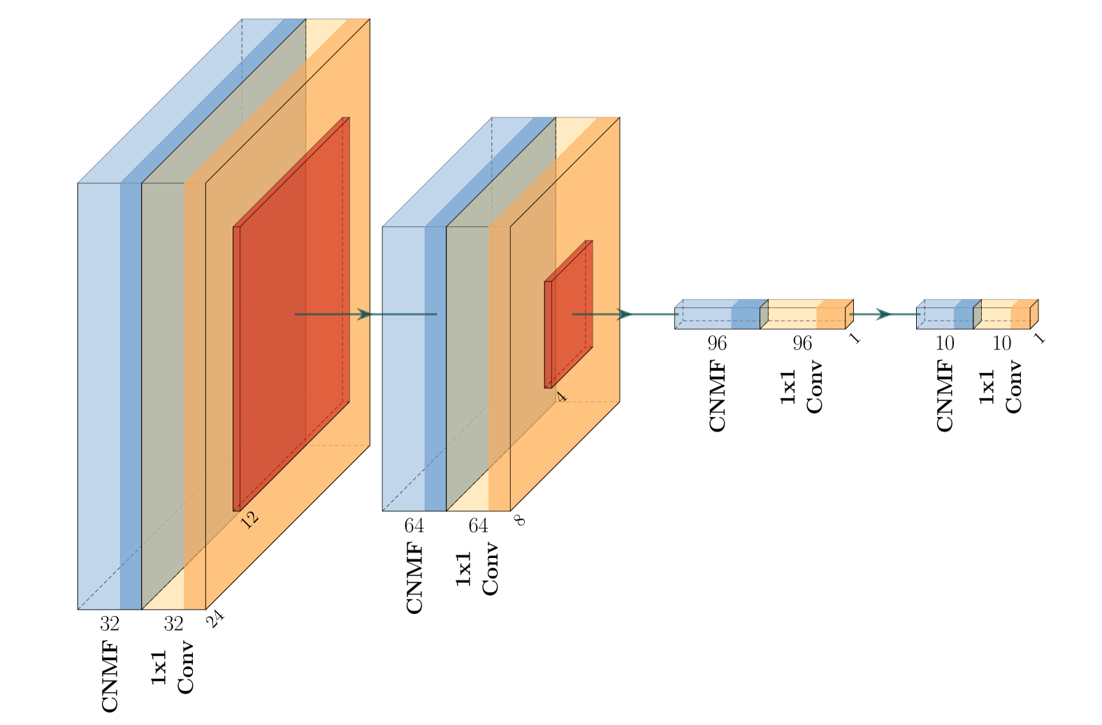
Figure 3 provides a detailed representation of our CNMF + convolution implementation (shown in Figure 4e), highlighting how the architecture progressively transforms the input through successive layers. For optimization purposes, we omit batch normalization in the final two blocks.
2.5.1 Loss Function
To optimize our models, we employed a composite loss function that combines cross-entropy (CE) loss with mean squared error (MSE). The loss function is defined as:
| (21) |
where represents the true label (one-hot encoded), represents the predicted probability distribution over classes, and is a weighting factor that balances the contribution of each component. While cross-entropy loss effectively optimizes for correct classification by heavily penalizing errors in the predicted class, it primarily focuses on the correct label and may not fully capture the relationship between incorrect predictions. By incorporating MSE with a smaller weight (), we introduce an additional regularizing term that considers the full distribution of predictions across all classes. This combined loss function led to consistent performance improvements across all model architectures in our experiments.
2.6 Implementation
All models were trained using the Adam optimizer with an initial learning rate of 0.001. To ensure optimal convergence, we implemented a learning rate reduction strategy where the rate was decreased by a factor of 10 whenever the validation loss plateaued for 10 consecutive epochs. The training was terminated either when the learning rate dropped below or when reaching the maximum limit of 500 epochs, whichever occurred first. For data augmentation, we applied random horizontal flips and color jitter to the training images. We also apply random crop on the input image from to . All hyperparameters were kept consistent across different model architectures to ensure a fair comparison. The models were implemented in PyTorch and trained on NVIDIA GeForce RTX 4090 GPU.
We evaluated the performance of our proposed model on the CIFAR-10 dataset, comparing them to a CNN and NMF model similar to those described in (Rotermund et al., 2023). The source containing all models and training setups can be found under: https://github.com/mahbodnr/deep_nmf
3 Results
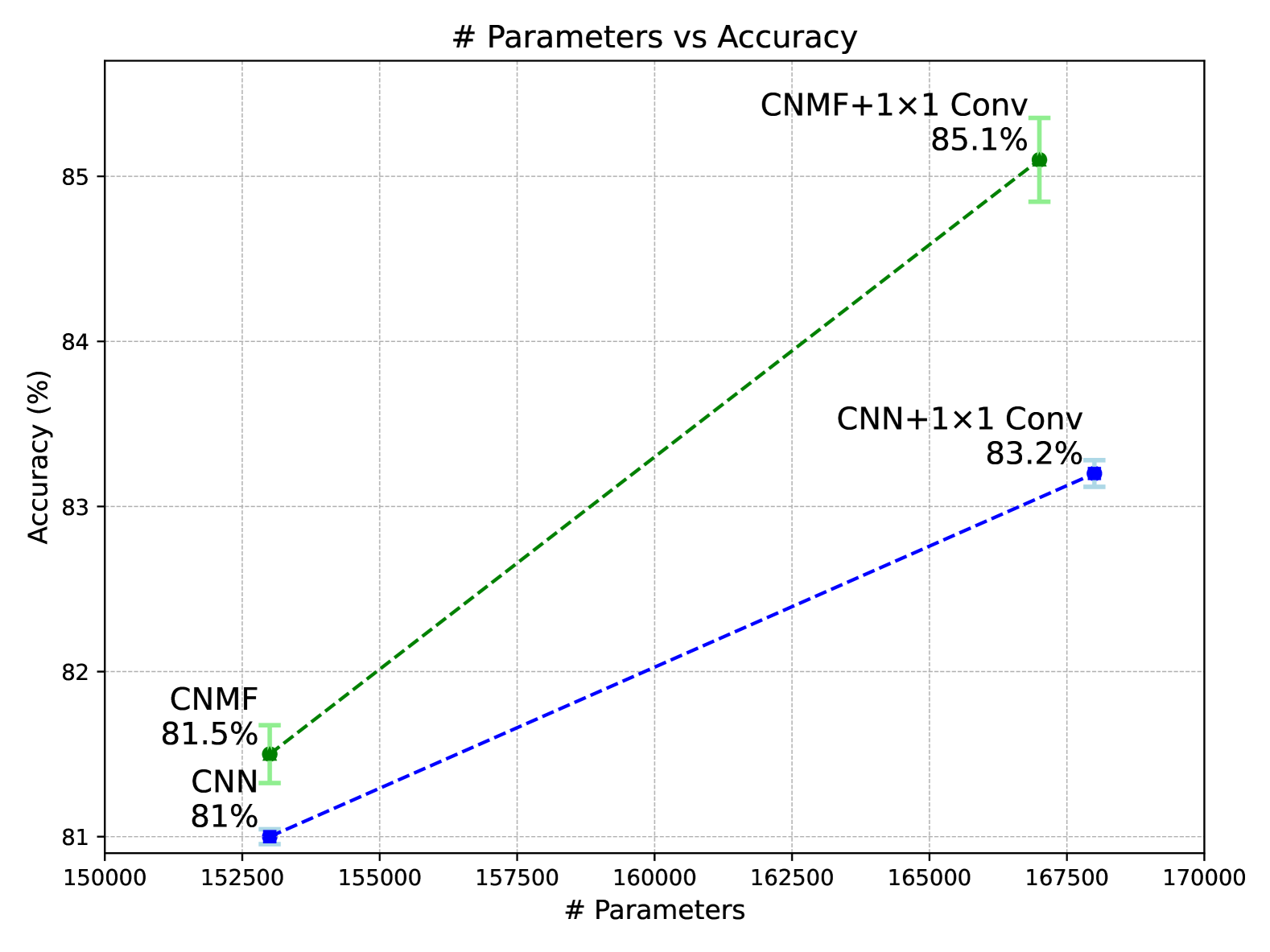
Figure 5 displays the classification accuracy achieved by all models on the CIFAR-10 dataset alongside their parameter counts. The results demonstrate that augmenting the CNMF model with convolutions substantially improves performance, allowing it to significantly outperform the baseline CNN model of comparable architecture and size.
3.1 Effect of NMF compared to CNN in the network
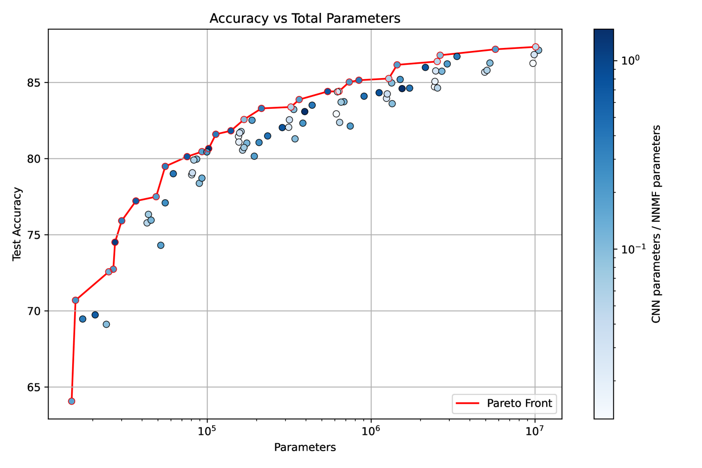
To investigate whether the performance improvements in our model stem primarily from the CNN components or if the NMF modules play a crucial role, we conducted an extensive analysis across different model configurations. We generated 100 different model variants by systematically adjusting the network architecture in two ways: first, by scaling the number of neurons in each layer (multiplying by factors of 2, 4, and 8), and second, by varying the number of groups in both NMF and CNN layers (using 1, 2, 4, 8, and 16 groups). When we increase the number of groups in a layer, we divide its channels into separate groups that process the input independently, thereby reducing the number of parameters while maintaining the same input and output dimensions. This approach allowed us to explore models with different ratios of NMF to CNN parameters while maintaining the overall architectural structure.
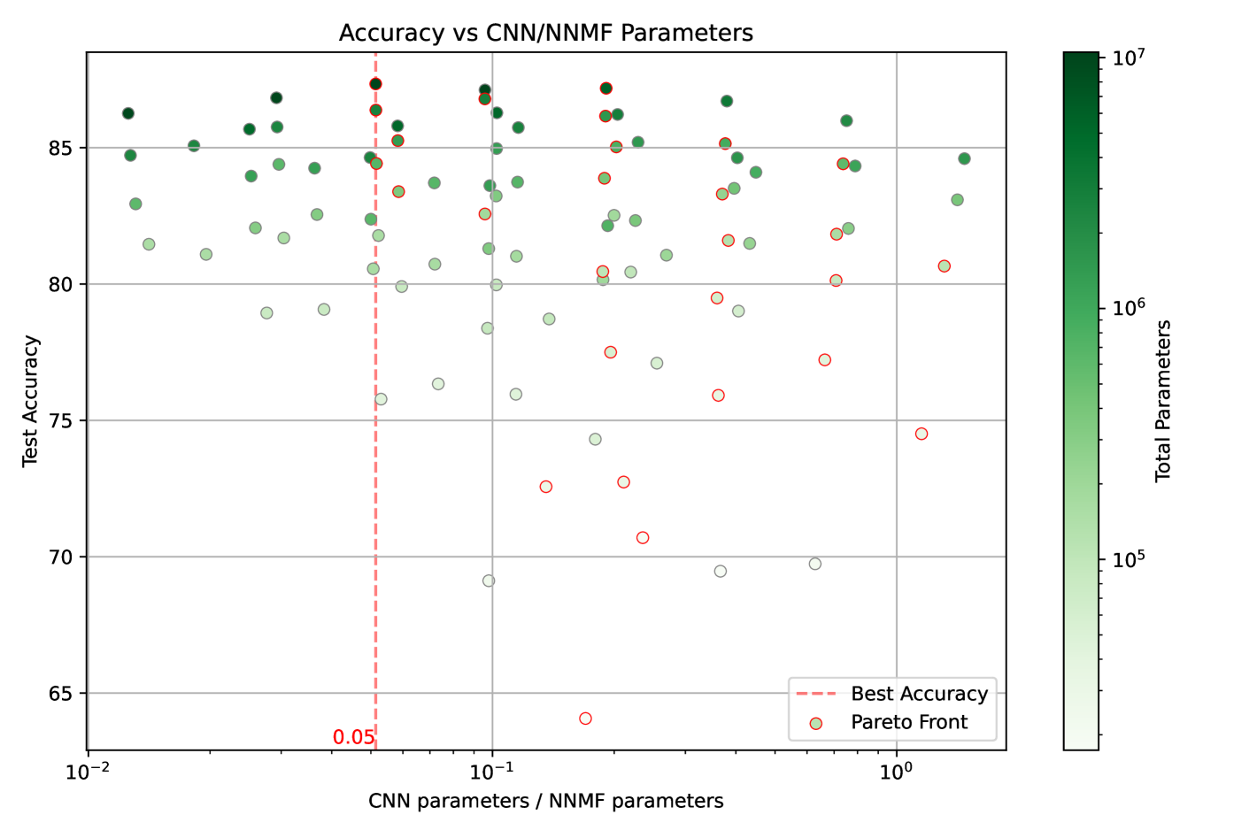
The results of this analysis are presented in Figure 3. The left panel shows model accuracy versus total parameter count, with the color intensity indicating the ratio of CNN to NMF parameters. The Pareto front, which represents the best-performing models for a given parameter budget, shows no systematic bias toward models with higher CNN parameter ratios. This suggests that simply increasing the proportion of CNN parameters does not lead to optimal performance. The right panel provides a complementary view, plotting accuracy against the ratio of CNN to NMF parameters, with color intensity representing the total parameter count. The distribution of high-performing models appears roughly symmetric around a balanced ratio, indicating that the best results are achieved when neither component dominates the network. Notably, the highest accuracy (indicated by the red dashed line) is achieved with a nearly balanced distribution of parameters between CNN and NMF components.
These findings strongly suggest that the NMF modules are not merely passive components but are essential contributors to the network’s performance. The optimal performance achieved with a balanced parameter distribution indicates a synergistic relationship between the NMF and CNN components, where each plays a crucial and complementary role in the network’s processing capabilities.
4 Discussion and Limitations
Our work demonstrates that incorporating biologically-inspired computational principles into deep neural networks can enhance their performance while maintaining biological plausibility. By combining NMF with local mixing through 1×1 convolutions, we achieved classification accuracy that matches or exceeds standard CNNs on the CIFAR-10 dataset, while preserving key biological constraints such as positive long-range interactions and local inhibitory processing.
4.1 Bridging Biological and Artificial Neural Computation
A fundamental distinction between biological neural computation and artificial neural networks lies in their computational dynamics. In biological systems, most neural processing occurs through implicit layers with complex recurrent interactions and iterative refinement of neural responses. This is evident in the cortical microcircuits where information is processed through multiple recursive loops between different neural populations before a stable representation emerges. In contrast, artificial neural networks predominantly rely on explicit feedforward computation, which, while computationally efficient, diverges significantly from biological reality.
Our approach bridges this gap by implementing NMF as an implicit layer that converges through iterative updates, more closely mimicking biological neural dynamics. While conventional feedforward networks like CNNs have dominated deep learning due to their computational efficiency and straightforward optimization, our results suggest that biologically inspired implicit computation can be equally effective when properly implemented. To make this happen, the key innovation in our work is the combination of iterative NMF processing with local feature mixing, which parallels the interaction between long-range excitatory connections and local inhibitory circuits in cortical processing.
4.2 Analysis of Feature Selection in NMF Networks
To understand the limitations of hierarchical NMF networks trained with unsupervised learning rules and subsequently fine-tuned for classification, it is helpful to decompose the input data into five distinct components:
-
1.
CD: Class-relevant Dominant statistical features
-
2.
CN: Class-relevant Non-dominant statistical features
-
3.
UD: class-Unrelated Dominant statistical features
-
4.
UN: class-Unrelated Non-dominant statistical features
-
5.
N: Noise
The key distinction between back-propagation and NMF’s local learning lies in their feature selection characteristics. Back-propagation, guided by the classification objective, effectively extracts both dominant and non-dominant class-relevant features (CD and CN). In contrast, NMF’s unsupervised learning rule, which optimizes for reconstruction based on statistical prominence, primarily captures dominant features regardless of their relevance to classification (CD and UD).
This fundamental difference creates a critical issue: when using NMF’s local learning rules instead of back-propagation, the non-dominant but class-relevant features (CN) are progressively filtered out as information flows through the network layers. By the time the signal reaches the output layer, these crucial classification features have been lost, despite their importance for the discrimination task. This explains the reduced classification performance observed in networks trained with NMF’s unsupervised learning rules. For example, a model with a similar architecture to our CNMF model will achieve accuracy when the NMF modules are trained only based on the local learning rule on the same task (as opposed to the that is achieved by using the back-propagation).
This analysis highlights why our approach of using supervised gradient descent to update the weights while maintaining NMF’s non-negativity constraints provides superior classification performance.
References
- Chen et al. (2022) Chen, W.S., Zeng, Q., Pan, B., 2022. A survey of deep nonnegative matrix factorization. Neurocomputing 491, 305–320. URL: http://dx.doi.org/10.1016/j.neucom.2021.08.152, doi:10.1016/j.neucom.2021.08.152.
- Ciampiconi et al. (2023) Ciampiconi, L., Elwood, A., Leonardi, M., Mohamed, A., Rozza, A., 2023. A survey and taxonomy of loss functions in machine learning. arXiv preprint arXiv:2301.05579 .
- Fukushima (1980) Fukushima, K., 1980. Neocognitron: A self-organizing neural network model for a mechanism of pattern recognition unaffected by shift in position. Biological Cybernetics 36, 193–202. URL: http://dx.doi.org/10.1007/BF00344251, doi:10.1007/bf00344251.
- Geng et al. (2021) Geng, Z., Guo, M.H., Chen, H., Li, X., Wei, K., Lin, Z., 2021. Is attention better than matrix decomposition? URL: https://arxiv.org/abs/2109.04553, doi:10.48550/ARXIV.2109.04553.
- Hoyer (2003) Hoyer, P.O., 2003. Modeling receptive fields with non-negative sparse coding. Neurocomputing 52-54, 547–552. URL: https://www.sciencedirect.com/science/article/pii/S0925231202007828, doi:https://doi.org/10.1016/S0925-2312(02)00782-8. computational Neuroscience: Trends in Research 2003.
- Hubel and Wiesel (1962) Hubel, D.H., Wiesel, T.N., 1962. Receptive fields, binocular interaction and functional architecture in the cat’s visual cortex. The Journal of Physiology 160, 106–154. URL: http://dx.doi.org/10.1113/jphysiol.1962.sp006837, doi:10.1113/jphysiol.1962.sp006837.
- Lecun et al. (1998a) Lecun, Y., Bottou, L., Bengio, Y., Haffner, P., 1998a. Gradient-based learning applied to document recognition. Proceedings of the IEEE 86, 2278–2324. doi:10.1109/5.726791.
- Lecun et al. (1998b) Lecun, Y., Bottou, L., Bengio, Y., Haffner, P., 1998b. Gradient-based learning applied to document recognition. Proceedings of the IEEE 86, 2278–2324. doi:10.1109/5.726791.
- Lee and Seung (2000) Lee, D., Seung, H.S., 2000. Algorithms for non-negative matrix factorization. Advances in neural information processing systems 13.
- Lee and Seung (1999) Lee, D.D., Seung, H.S., 1999. Learning the parts of objects by non-negative matrix factorization. Nature 401, 788–791. URL: http://dx.doi.org/10.1038/44565, doi:10.1038/44565.
- Olshausen and Field (1996) Olshausen, B.A., Field, D.J., 1996. Emergence of simple-cell receptive field properties by learning a sparse code for natural images. Nature 381, 607–609. URL: http://dx.doi.org/10.1038/381607a0, doi:10.1038/381607a0.
- Olshausen and Field (2006) Olshausen, B.A., Field, D.J., 2006. What is the other 85 percent of v1 doing. L. van Hemmen, & T. Sejnowski (Eds.) 23, 182–211.
- Rotermund et al. (2023) Rotermund, D., Garcia-Ortiz, A., Pawelzik, K.R., 2023. Competitive performance and superior noise robustness of a non-negative deep convolutional spiking network. Neurosomething URL: http://dx.doi.org/10.1101/2023.04.22.537923, doi:10.1101/2023.04.22.537923.
- Rotermund and Pawelzik (2019) Rotermund, D., Pawelzik, K.R., 2019. Back-propagation learning in deep spike-by-spike networks. Frontiers in Computational Neuroscience 13, 55.
- Strata and Harvey (1999) Strata, P., Harvey, R., 1999. Dale’s principle. Brain Research Bulletin 50, 349–350. URL: http://dx.doi.org/10.1016/S0361-9230(99)00100-8, doi:10.1016/s0361-9230(99)00100-8.
- Tian et al. (2022) Tian, Y., Su, D., Lauria, S., Liu, X., 2022. Recent advances on loss functions in deep learning for computer vision. Neurocomputing 497, 129–158.
- Yang et al. (2013) Yang, W., Carrasquillo, Y., Hooks, B.M., Nerbonne, J.M., Burkhalter, A., 2013. Distinct balance of excitation and inhibition in an interareal feedforward and feedback circuit of mouse visual cortex. The Journal of Neuroscience 33, 17373–17384. URL: http://dx.doi.org/10.1523/JNEUROSCI.2515-13.2013, doi:10.1523/jneurosci.2515-13.2013.