Abstract

We address the challenge of sequential data-driven decision-making under context distributional uncertainty. This problem arises in numerous real-world scenarios where the learner optimizes black-box objective functions in the presence of uncontrollable contextual variables. We consider the setting where the context distribution is uncertain but known to lie within an ambiguity set defined as a ball in the Wasserstein distance. We propose a novel algorithm for Wasserstein Distributionally Robust Bayesian Optimization that can handle continuous context distributions while maintaining computational tractability. Our theoretical analysis combines recent results in self-normalized concentration in Hilbert spaces and finite-sample bounds for distributionally robust optimization to establish sublinear regret bounds that match state-of-the-art results. Through extensive comparisons with existing approaches on both synthetic and real-world problems, we demonstrate the simplicity, effectiveness, and practical applicability of our proposed method.

1 INTRODUCTION

Bayesian Optimization (BO) has emerged as a powerful algorithm for zero-order optimization of expensive-to-evaluate black-box functions, with applications ranging from hyperparameters tuning to scientific discovery and robotics (Ueno et al., 2016; Li et al., 2019; Ru et al., 2020; Shahriari et al., 2015). In the standard BO setting, the learner sequentially selects points to evaluate the unknown objective function and uses the observed data to update a surrogate model that captures the function’s behavior. In the contextual BO setting, the objective function depends on an additional variable, called the context, which cannot be controlled by the learner (Krause and Ong, 2011; Valko et al., 2013; Kirschner and Krause, 2019). Typically, the context distribution is used to model the uncertainty of the learner related to uncontrollable environmental variables. When the distribution of the context variable is known, the BO algorithm can be used to solve the Stochastic Optimization (SO) problem, where the objective is to maximize the reward of the unknown function in expectation with respect to the context distribution

$$\max_{x\in\mathcal{X}}\mathbb{E}_{c\sim\mathcal{P}}[f(x,c)]\ .$$

However, in many real-world scenarios, the learner does not have access to the true context distribution, but only to an approximate one. This can happen, e.g., when the context distribution is estimated from historical data, and only a finite number of samples are available. This results in a distributional mismatch between the distribution available to the learner for optimization and the true distribution of the context variable. To formally account for the effect of the distributional mismatch, Distributionally Robust Optimization (DRO) has recently gained considerable attention, especially in the sampled data settings (Rahimian and Mehrotra, 2019; Kuhn et al., 2019; Gao et al., 2024). In DRO, the learner optimizes the reward under the worst-case distribution of the context within a so-called ambiguity set $\mathcal{B}$ that captures the uncertainty of the learner about the true context distribution

$$\max_{x\in\mathcal{X}}\inf_{\mathcal{Q}\in\mathcal{B}}\mathbb{E}_{c\sim\mathcal{Q}}[f(x,c)]\ .$$ (1)

The advantage of the robust approach is that, by appropriately choosing the ambiguity set $\mathcal{B}$, we can guarantee that the reward computed for the DRO problem lower-bounds the reward for the true unknown context distribution.

In this work, we introduce Wasserstein Distributionally Robust Bayesian Optimization (WDRBO), a novel algorithm that combines the principles of BO and DRO to address the challenge of sequential data-driven decision-making under context distributional uncertainty. We consider ambiguity sets defined as balls in the Wasserstein distance (Kuhn et al., 2019) which allows for a flexible and intuitive way to model the uncertainty in the context distribution. We design a computationally tractable algorithm and analyze its performance in two settings: the General WDRBO setting, where at each time-step the Wasserstein ambiguity set is provided to the learner, and the Data-Driven WDRBO setting, in which we assume that the true context distribution is time-invariant and the Wasserstein ambiguity set is built using the past context observations.

Our main contributions are as follows:

• We propose a novel, computationally tractable algorithm for Wasserstein Distributionally Robust Bayesian Optimization that handles continuous context distributions. Our approach exploits an approximate reformulation based on Lipschitz bounds of the acquisition function, circumventing the need for context discretization.

• We establish a cumulative expected regret bound of order $\tilde{O}(\sqrt{T}\gamma_{T})$ for the general WDRBO setting, where $T$ is the number of iterations and $\gamma_{T}$ is the maximum information gain. For the data-driven setting, we obtain sublinear regret guarantees without requiring assumptions on the rate of decay of the ambiguity set radius.

• We derive novel Lipschitz bounds for the mean and variance estimates, and leverage recent finite-sample bounds for Wasserstein DRO to address the dimensionality challenges in continuous context spaces.

• We provide comprehensive empirical evaluations on synthetic and real-world problems, demonstrating that our method achieves competitive performance with significantly lower computational complexity compared to existing DRBO approaches.

The rest of the paper is organized as follows. In Section 2, we review related work. In Section 3, we introduce the problem formulation. In Section 4, we present the proposed algorithm and provide the theoretical analysis. In Section 5, we present the experimental results. Finally, in Section 6, we conclude the paper and discuss future work.

2 RELATED WORK

The foundation of DRBO was laid by Kirschner et al. (2020), who introduced the concept of distributional robustness in BO. They propose a BO formulation that is robust to the worst-case context distribution within an ambiguity set defined by the Maximum Mean Discrepancy (MMD) distance. While groundbreaking, the inner worst-case calculation requires at each iteration the solution of a convex optimization problem that renders this approach computationally viable only when the context space is discrete and with low cardinality. A quadrature-based scheme for DRBO is proposed in Nguyen et al. (2020), but their algorithm is limited to the simulator setting where at each iteration the learner is allowed to choose the context. Husain et al. (2024) develops a DRBO formulation for $\ phi$-divergence-based ambiguity sets, but their formulation has some implicit requirements on the support of the distributions captured by the ambiguity set. Recognizing these computational limitations, Tay et al. (2022) proposed a set of approximate techniques using worst-case sensitivity analysis based on Taylor’s expansions. These methods offer better computational complexity for multiple descriptions of ambiguity sets at the expense of performance and regret bounds that scale linearly with the worst-case sensitivity approximation error. To avoid the challenges of context space discretization, Huang et al. (2024) proposes a kernel density estimation step that uses the available context samples to estimate a continuous context distribution. The estimated context distribution is then sampled and the samples are used in a DRBO formulation where the $\phi$-divergence ambiguity sets capture the distributional uncertainty introduced by the density estimation step.

The regret analysis of the existing literature on DRBO builds on the GP-UCB formulation of Srinivas et al. (2009, 2012), we instead exploit self-normalizing concentration bounds in Reproducing Kernel Hilbert Space (RKHS) (Abbasi-Yadkori, 2013; Kirschner et al., 2020; Whitehouse et al., 2023). We address a gap in the DRBO literature and analyze the continuous context distribution setting under the Wasserstein-based ambiguity set. We leverage recent advancements in Wasserstein DRO literature (Gao, 2023; Gao et al., 2024) to provide state-of-the-art regret rates in the data-driven setting.

3 PROBLEM FORMULATION

We consider an unknown objective function $f:\mathcal{X}\times\mathcal{C}\rightarrow\mathbb{R}$, where $\mathcal{X}\subset\mathbb{R}^{d_{x}}$ is the input space and $\mathcal{C}\subset\mathbb{R}^{d_{c}}$ is the context space. The learner’s goal is to maximize the expected value of the function under the context distribution by sequentially selecting points to evaluate and receiving noisy observations of the function. More specifically, at each iteration $t=1,2,\ldots$, the learner selects a point $x_{t}\in\mathcal{X}$ to query the function, and observes the context $c_{t}\in\mathcal{C}$ and a noisy output $y_{t}=f(x_{t},c_{t})+\eta_{t}$. The context sample $c_{t}$ is assumed to be an independent sample from some unknown, time-dependent, context distribution $\mathcal{P}^{*}_{t}$, while $\eta_{t}$ is a zero-mean $R$-sub-Gaussian noise, where an upper bound on $R$ is known.

3.1 Wasserstein Distributionally Robust Objective

In this work, we consider the setting of distributionally robust optimization, where the learner does not have access to the true context distribution $\mathcal{P}^{*}_{t}$, but instead optimizes for the expected reward under the worst-case distribution within an ambiguity set

$$\max_{x\in\mathcal{X}}\inf_{\mathcal{Q}\in\mathcal{B}^{\varepsilon_{t}}(\hat{\mathcal{P}}_{t})}\mathbb{E}_{c\sim\mathcal{Q}}[f(x,c)]\ .$$ (2)

The time-dependent ambiguity set $\mathcal{B}^{\varepsilon_{t}}(\hat{\mathcal{P}}_{t})$ is defined as a ball in the Wasserstein distance centered at the distribution $\hat{\mathcal{P}}_{t}$ and with radius $\varepsilon_{t}$ (Kuhn et al., 2019). This is the set of all distributions that are within a Wasserstein distance $\varepsilon_{t}$ from the center distribution $\hat{\mathcal{P}}_{t}$

$$\mathcal{B}^{\varepsilon_{t}}(\hat{\mathcal{P}}_{t})=\left\{\mathcal{Q}\in\mathcal{P}(\mathcal{C}):d_{W}(\mathcal{Q},\hat{\mathcal{P}}_{t})\leq\varepsilon_{t}\right\}.$$

The type-1 Wasserstein metric $d_{\mathrm{W}}:\mathcal{M}(\mathbb{Q})\times\mathcal{M}(\mathbb{Q})\rightarrow\mathbb{R}_{\geq 0}$ defines the distance between two distributions $\mathcal{Q}_{1}$ and $\mathcal{Q}_{2}$ as

$$d_{W}\left(\mathcal{Q}_{1},\mathcal{Q}_{2}\right):=\inf_{\Pi}\left\{\int_{\mathbb{Q}\times\mathbb{Q}}\left\|{\bm{q}}_{1}-{\bm{q}}_{2}\right\|\Pi\left(\mathrm{d}{\bm{q}}_{1},\mathrm{d}{\bm{q}}_{2}\right)\right\},$$

where the transportation map $\Pi$ takes values in the set of joint distributions of ${\bm{q}}_{1}$ and ${\bm{q}}_{2}$ with marginals $\mathcal{Q}_{1}$ and $\mathcal{Q}_{2}$, and $\|\cdot\|$ is the euclidean norm.

3.2 Regularity Assumptions and Surrogate Model

The BO algorithm maintains a surrogate model of the objective function, which is used to guide the selection of the next query point. We use a regularized least squares estimator of the function $f$ in the RKHS(Abbasi-Yadkori, 2013; Kirschner and Krause, 2018) under the assumption that $f$ is an unknown fixed member of the RKHS $\mathcal{H}_{k}$ that is specified by the positive semi-definite kernel $k:\mathcal{Z}\times\mathcal{Z}\rightarrow\mathbb{R}$, where $\mathcal{Z}=\mathcal{X}\times\mathcal{C}$. Here we define $z=[x^{\top},c^{\top}]^{\top}$ to keep the notation compact. We assume that the spaces $\mathcal{X}$ and $\mathcal{C}$ are compact. We define the norm of a function $g\in{\mathcal{H}_{k}}$ as $\|g\|_{\mathcal{H}_{k}}=\sqrt{g^{\top}g}=\sqrt{\langle g,g\rangle_{\mathcal{H}_{k}}}$. We also assume that the unknown function $f$ has bounded RKHS norm, i.e., $\|f\|_{\mathcal{H}_{k}}\leq B$, for some $B>0$, and that the kernel $k$ is bounded, i.e., $k(z,z^{\prime})\leq 1$, for all $z,\ z^{\prime}\in\mathcal{Z}$. The assumptions made here are common in the BO literature, we point the reader to e.g. Bogunovic and Krause (2021) for the analysis of bandits optimization with misspecified RKHS. The details of the following derivations are available in the Appendix Section 7.

Given the dataset $\mathcal{D}_{t}=\{(z_{i},y_{i})\}_{i=1}^{t}$, and regularization parameter $\lambda>0$, the regularized least-squares regression problem in RKHS is written as follows:

$$\min_{\mu\in{\mathcal{H}_{k}}}\sum_{i=1}^{t}\left(y_{i}-\mu(z_{i})\right)^{2}+\lambda\|\mu\|_{\mathcal{H}_{k}}^{2}.$$ (3)

The resulting least squares estimator is

$$\mu_{t}(z)=k_{t}(z)^{\top}(K_{t}+\lambda I)^{-1}y_{1:t}\ ,$$ (4)

where $k_{t}(z)=[k(z,z_{1}),\ldots,k(z,z_{t})]^{\top}$, $K_{t}=[k(z_{i},z_{j})]_{i,j=1}^{t}$, and $y_{1:t}=[y_{1},\ldots,y_{t}]^{\top}$. We also define

$$\sigma_{t}^{2}(z)=\frac{1}{\lambda}\left(k(z,z)-k_{t}(z)^{\top}(K_{t}+\lambda I)^{-1}k_{t}(z)\right)\ .$$ (5)

Under suitable assumptions on the prior and the noise distribution, $\mu_{t}$ and $\sigma_{t}^{2}$ correspond to the posterior mean and variance of a Gaussian process with kernel $k$ conditioned on the observations $y_{1:t}$ (Schölkopf and Smola, 2002; Williams and Rasmussen, 2006).

We state here a fundamental result adapted from Abbasi-Yadkori (2013) that provides probabilistic finite-sample confidence guarantees for the least squares estimator (4).

Lemma 1.

[(Abbasi-Yadkori, 2013, Th. 3.11)] Let $\mathcal{Z}\subset\mathbb{R}^{d}$, where $d=d_{x}+d_{c}$, and $f:\mathcal{Z}:\rightarrow\mathbb{R}$ be a member of ${\mathcal{H}_{k}}$, with $\|f\|_{\mathcal{H}_{k}}\leq B$, and let $\eta_{t}$ be $\mathcal{F}_{t}$ measurable and $R$-sub-Gaussian conditionally on $\mathcal{F}_{t}$. Then, for any $\lambda>0$, with probability $1-\delta$, we have that for all $z\in\mathcal{Z}$ and all $t\geq 1$:

$$|\mu_{t-1}(z)-f(z)|\leq\beta_{t}\sigma_{t-1}(z)\ ,$$ (6)

with

$$\beta_{t}:=R\sqrt{2\log\left(\frac{\det(I+\lambda^{-1}K_{t-1})^{\frac{1}{2}}}{\delta}\right)}+\lambda^{\frac{1}{2}}B\ ,$$ (7)

where $\mu_{t-1}$ and $\sigma_{t-1}$ are defined as in equations (4),(5).

We also introduce here the maximum information gain (Srinivas et al., 2009; Chowdhury and Gopalan, 2017; Vakili et al., 2021), a fundamental kernel-dependent quantity that quantifies the complexity of learning in RKHS

$$\gamma_{t}:=\sup_{z_{1},z_{2},\dots,z_{t}}\log\det\left(I+\lambda^{-1}K_{t-1}\right)\ .$$

In order to derive the main results in the following sections, we require the kernel to satisfy the following Lipschitz property

Assumption 1 (Lipschitz property).

There exists a $L>0$ such that for any $z,z^{\prime}\in\mathcal{X}\times\mathcal{C}$, $d(z,z^{\prime}):=\|k(\cdot,z)-k(\cdot,z^{\prime})\|_{\mathcal{H}_{k}}\leq L\|z-z^{\prime}\|$ .

As we prove in Lemma 11 in the Appendix, Assumption 1 is verified for popular kernels, e.g. the squared exponential kernel, and some kernels in the Matérn family satisfy.

4 WASSERSTEIN DISTRIBUTIONALLY ROBUST BAYESIAN OPTIMIZATION

In classical BO, following the rich literature of optimism in the face of uncertainty, the learner selects the query point $x_{t}$ by maximizing the Upper Confidence Bound (UCB) function (Auer, 2002). This provides a trade-off between exploration and exploitation, and results in provable regret guarantees (Srinivas et al., 2009).

Departing from the classical approach, and inspired by Kirschner et al. (2020), we adopt a robust approach, where we consider the optimization of a robustified version of the UCB function

$$x_{t}=\arg\max_{x\in\mathcal{X}}\inf_{\mathcal{Q}\in\mathcal{B}^{\varepsilon_{t}}(\hat{\mathcal{P}}_{t})}\mathbb{E}_{c\sim\mathcal{Q}}\left[UCB_{t}(x,c)\right]\ ,$$ (8)

where

$$UCB_{t}(x,c)=\mu_{t-1}(x,c)+\beta_{t}\sigma_{t-1}(x,c),$$ (9)

with $\mu_{t}$, $\sigma_{t}$, and $\beta_{t}$ are given in (4), (5), (7) respectively.

Similar to Kirschner et al. (2020), we will analyze two settings, which differ in the way the ambiguity set is obtained. We first consider the General WDRBO setting, where at each time-step the Wasserstein ambiguity set is provided to the learner, and then turn to the Data-Driven WDRBO setting, in which the Wasserstein ambiguity set is built using the past context observations under the assumption that the true context distribution is time-invariant.

All proofs along with supporting derivations and lemmas are provided in Section 8 of the Appendix.

To evaluate the performance of the proposed algorithm we look at the notion of regret. Regret is used to capture the difference in performance between some algorithm and a benchmark algorithm that has access to privileged information. The definition of regret and the choice of benchmark is not unique, and the one chosen here differs from the ones used in the DRBO literature  Kirschner and Krause (2019), Husain et al. (2024), Tay et al. (2022).

We will consider the following definitions of instantaneous expected regret:

$$r_{t}=\mathbb{E}_{c\sim\mathcal{P}^{*}_{t}}{[f(x^{*}_{t},c)]}-\mathbb{E}_{c\sim\mathcal{P}^{*}_{t}}{[f(x_{t},c)]}\ ,$$ (10)

and cumulative expected regret:

$$R_{T}=\sum_{t=1}^{T}r_{t}\ .$$ (11)

The benchmark solution $x^{*}_{t}$ is the optimal solution to the true stochastic optimization problem at time-step $t$, given access to the true function $f$ and context distribution $\mathcal{P}^{*}_{t}$, i.e.,

$$x^{*}_{t}=\arg\max_{x\in\mathcal{X}}\mathbb{E}_{c\sim\mathcal{P}^{*}_{t}}{[f(x,c)]}\ .$$

Hence, this definition of regret captures the (cumulative) sub-optimality gap, between some proposed algorithm and the optimal solution to the true stochastic optimization problem.

4.1 General WDRBO

In the General WDRBO setting, at each time-step $t$, the center $\hat{\mathcal{P}}_{t}$ and the radius $\varepsilon_{t}$ of the Wasserstein ambiguity set are provided to the learner. This represents the setting where there is some understanding of what the context distribution is, e.g. with weather or prices forecast, but there is still some uncertainty about its distribution.

To make the robust problem 8 tractable, we introduce a well-known result from the Wasserstein DR optimization literature (Kuhn et al., 2019; Gao et al., 2024) that has been adapted to our problem.

Lemma 2.

Let $f:\mathcal{X}\times\mathcal{C}\rightarrow\mathbb{R}$ be a function that is $L^{f}_{c}(x)$-Lipschitz in the context space, i.e. $|f(x,c)-f(x,c^{\prime})|\leq L^{f}_{c}(x)\|c-c^{\prime}\|$, for all $c,c^{\prime}\in\mathcal{C}$. Let $\mathcal{B}^{\varepsilon}(\hat{\mathcal{P}})$ be a Wasserstein ambiguity set defined as a ball of radius $\varepsilon$ in the Wasserstein distance centered at the distribution $\hat{\mathcal{P}}$. Then, for any $x\in\mathcal{X}$ and for any distribution $\tilde{\mathcal{P}}\in\mathcal{B}^{\varepsilon}(\hat{\mathcal{P}})$, we have that

$$|\mathbb{E}_{c\sim\tilde{\mathcal{P}}}[f(x,c)]-\mathbb{E}_{c\sim\hat{\mathcal{P}}}[f(x,c)]|\leq\varepsilon L^{f}_{c}(x)\ .$$ (12)

Lemma 2 provides a simple Lipschitz-based bound on the worst-case expectation for any distribution in the ambiguity set. By combining Lemma 2 with Assumption 1 we obtain a tractable approximation of the robust maximization problem 8. Thus, at each time-step $t$ the query point $x_{t}$ is selected by the following acquisition function

$$x_{t}=\arg\max_{x\in\mathcal{X}}\mathbb{E}_{c\sim\hat{\mathcal{P}}_{t}}\left[\text{UCB}_{t}(x,c)\right]-\varepsilon_{t}L^{\text{UCB}_{t}}(x)\,,$$ (13)

where $L^{\text{UCB}_{t}}(x)$ is the Lipschitz constant of the function $\text{UCB}_{t}$ with respect to the context variable $c$, evaluated at $x$. The resulting algorithm for WDRBO is provided in Algorithm 1.

Algorithm 1 General Algorithm for WDRBO

 for $t=1$ to $T$ do

  $\mu_{t-1},\ \sigma_{t-1}\leftarrow\text{fit}(\mathcal{D}_{t-1})$

  $x_{t}=\arg\max_{x\in\mathcal{X}}\mathbb{E}_{c\sim\hat{\mathcal{P}}}[\text{UCB}_{t}(x,c)]-\varepsilon_{t}L^{\text{UCB}_{t}}(x)$

  The environment returns $c_{t}$ and $y_{t}=f(x_{t},c_{t})+\eta_{t}\$, where $c_{t}\sim\mathcal{P}^{*}_{t}\in\mathcal{B}^{\varepsilon_{t}}(\hat{\mathcal{P}}_{t})$

  $\mathcal{D}_{t}\leftarrow\mathcal{D}_{t-1}\cup\{(x_{t},c_{t},y_{t})\}$

 end for

We remark that, unlike the algorithm proposed in Kirschner and Krause (2019), Husain et al. (2024), Tay et al. (2022), that rely on discrete context distributions, neither Algorithm 1 nor the following theoretical analysis require a discrete context space or that the distributions in the ambiguity have finite support. The only practical limitation imposed by our algorithm when the center is a continuous context distribution, is the ability to perform the numerical integration required to compute the expectation.

While in Algorithm 1 the Lipschitz constant $L^{\text{UCB}_{t}}(x)$ can be computed at each timestep $t$ from the fitted UCB function $\text{UCB}_{t}$, in the following lemma we derive a novel upper bound on $L^{\text{UCB}_{t}}(x)$ that will be useful for the theoretical analysis of the regret.

Lemma 3.

Let $0<\delta<1$ be a failure probability and let $\bar{B}_{t}:=\lambda^{-\frac{1}{2}}R\sqrt{2\log\left(\frac{\det(I+\lambda^{-1}K_{t-1})^{\frac{1}{2}}}{\delta}\right)}+B\leq\lambda^{-\frac{1}{2}}\left(\left(R\sqrt{2\log\frac{1}{\delta}}+R\sqrt{2\gamma_{t}}\right)+B\right)$ .

Then, with probability $1-\delta$ for all $t\geq 1$ we have $\|\mu_{t-1}\|_{\mathcal{H}_{k}}\leq\bar{B}_{t}.$ Further, if Assumption 1 holds we have:

(i) With probability $1-\delta$, for any $z,z^{\prime}\in\mathcal{X}\times\mathcal{C}$: $|\mu_{t-1}(z)-\mu_{t-1}(z^{\prime})|\leq\bar{B}_{t}L\|z-z^{\prime}\|.$

(ii) For any $z,z^{\prime}\in\mathcal{X}\times\mathcal{C}$: $|\beta_{t}\sigma_{t-1}(z)-\beta_{t}\sigma_{t-1}(z^{\prime})|\leq\beta_{t}\lambda^{-\frac{1}{2}}L\|z-z^{\prime}\|=\bar{B}_{t}L\|z-z^{\prime}\|.$

Therefore, with probability $1-\delta$, the UCB function is Lipschitz continuous with constant:

$$L^{\text{UCB}_{t}}\leq 2\bar{B}_{t}L.$$

We can now turn to the derivation of the bound on the instantaneous expected regret for the General WDRBO setting.

Theorem 4 (Instantaneous expected regret).

Let Assumption 1 hold. Fix a failure probability $0<\delta<1$. With probability at least $1-\delta$, for all $t\geq 1$ the instantaneous expected regret can be bounded by

$$r_{t}\leq\mathbb{E}_{c\sim\mathcal{P}^{*}_{t}}\left[2\beta_{t}\sigma_{t-1}(x_{t},c)\right]+2\varepsilon_{t}L^{\text{UCB}_{t}}(x^{*}_{t})$$ (14)

We can observe that the first term has the same expression as the instantaneous regret of the GP-UCB Srinivas et al. (2009), while the second term captures the effect of the distributional uncertainty which depends on the maximum distribution shift as specified by $\varepsilon_{t}$, and on a sensitivity term that is bounded by the Lipschitz constants $L^{\text{UCB}_{t}}(x_{t})$ computed at the selected input $x_{t}$.

Theorem 5 (Cumulative expected regret).

Let Assumption 1 hold and let $L^{\text{UCB}_{t}}(x)$ be a Lipschitz constant with respect to the context $c$ for $\text{UCB}_{t}(x,c)$. Fix a failure probability $0<\delta<1$. With probability at least $1-2\delta$, the cumulative expected regret after $T$ steps can be bounded as:

$$R_{T}\leq 4\beta_{T}\sqrt{T\gamma_{T}+4\log(\frac{6}{\delta})}+\sum_{t=1}^{T}\varepsilon_{t}2L^{\text{UCB}_{t}}(x^{*}_{t})\ ,$$ (15)

where $\gamma_{T}$ is the maximum information gain at time $T$.

Note that the cumulative expected regret is a random quantity, as the expectation is taken only with respect to the contexts. We can combine Lemma 3 with Theorem 5 to derive the regret rate for the cumulative expected regret.

Corollary 6 (General WDRBO Regret Order).

Let $0<\delta<1$ be a failure probability and let Assumption 1 hold. Then, with probability $1-2\delta$, the cumulative expected regret is of the order of

$$R_{T}=\tilde{O}\left(\sqrt{T}\gamma_{T}+\sqrt{\gamma_{T}}\sum_{t=1}^{T}\varepsilon_{t}\right)\ .$$

For the Squared Exponential kernel, this reduces to

$$R_{T}=\tilde{O}\left(\sqrt{T}+\sum_{t=1}^{T}\varepsilon_{t}\right)\ ,$$

where $\tilde{O}$ omits logarithmic terms.

The second term depends on the sum of all radii $\sum_{t=1}^{T}\varepsilon_{t}$. Hence, a sufficient condition in order to get sublinear regret guarantees, is that the radii converge to $0$ sufficiently fast. If, e.g., $\varepsilon_{t}=O(t^{-\frac{1}{2}})$, we obtain $R_{T}=\tilde{O}\left(\sqrt{T}\gamma_{T}\right)$. This can also occur in certain situations like the data-driven setting that we analyze next.

4.2 Data-Driven WDRBO

In the Data-Driven WDRBO we still rely on Algorithm 1, but differently from the general setting we need to build the Wasserstein ambiguity set using the past context observations. With the assumption that the unknown context distribution is time-invariant, i.e. $\mathcal{P}^{*}_{t}:=\mathcal{P}^{*}$, $t\in 1,\dots,T$, we build the ambiguity set center $\hat{\mathcal{P}}_{t}$ as the empirical distribution of the past observed contexts, i.e.

$$\hat{\mathcal{P}}_{t}=\frac{1}{t}\sum_{i=1}^{t}\mathcal{I}_{\{c=c_{i}\}}\ ,$$

where $\mathcal{I}_{\{c=c^{i}\}}$ is the indicator function centered on the context sample $c^{i}$, and we derive a bound on the sequence of radii $\varepsilon_{t}$ using finite-sample concentration results.

Using finite-sample results for the convergence of empirical measures in Wasserstein distance Fournier and Guillin (2015); Fournier (2022) it is possible to bound the size of $\varepsilon_{t}$ such that with high probability the true context distribution $\mathcal{P}^{*}$ is contained in the ambiguity set $\mathcal{B}^{\varepsilon_{t}}(\hat{\mathcal{P}}_{t})$. Unfortunately, this approach suffers from the so-called curse of dimensionality with respect to the dimension $d_{c}$ of the context. To circumvent this issue we propose a novel result that leverages recent finite-sample concentration results from Gao (2023). Instead of focusing on the rate of convergence of the empirical distribution $\hat{\mathcal{P}}_{t}$ to the true unknown $\mathcal{P}^{*}$, we focus on the rate at which the worst-case expected cost concentrates around the expected cost under the true context distribution.

To extend the result of Gao (2023) to the WDRBO setting we require an additional covering argument over all possible UCB functions, which depend on all the possible sampling histories of the algorithm. Define the class of functions

$$\mathcal{U}(m,b,s)= \left\{h:h(z)=\mu(z)+\beta\sigma(z)\ ,\right.$$

$$\left.\|\mu\|_{\mathcal{H}_{k}}\leq m,\ \beta\leq b,\ \sigma(z)\in{\bm{\sigma}}_{s}\right\}\ ,$$

where

$${\bm{\sigma}}_{s}=\left\{\sigma:\sigma(z)=\|\mathcal{M}k(\cdot,z)\|_{\mathcal{H}_{k}},\ \|\mathcal{M}\|_{op}\leq s^{-\frac{1}{2}}\right\}\ .$$

Let $\mathcal{N}_{\infty}(\rho,\mathcal{U}(m,b,s))$ be its covering number under the infinity norm, up to precision $\rho$. Let ${\mathrm{D}_{\mathcal{X}}}$, ${\mathrm{D}_{\mathcal{C}}}$ denote the diameters of the sets $\mathcal{X},\mathcal{C}$ respectively.

Lemma 7.

Let $0<\delta<1$ be a failure probability, and let $\text{UCB}_{t}(x,c)=\mu_{t-1}(x,c)+\beta_{t}\sigma_{t-1}(x,c)\in\mathcal{U}(\bar{B}_{t},\bar{B}_{t},\lambda)$. Then, with probability at least $1-2\delta$, for any $x\in\mathcal{X}$ we have:

$$\left|\mathbb{E}_{c\sim\mathcal{P}^{*}}[\text{UCB}_{t}(x,c)]-\mathbb{E}_{c\sim\hat{\mathcal{P}}_{t}}[\text{UCB}_{t}(x,c)]\right|\leq$$

$$\qquad\qquad\qquad\leq\varepsilon_{t}L^{\text{UCB}}_{t}(x)+\rho_{t},$$

where

$$\varepsilon_{t}\!=\!\sqrt{2{\mathrm{D}_{\mathcal{C}}}^{2}\frac{\log 1/\delta\!+\!d_{x}\log(1+2t{\mathrm{D}_{\mathcal{X}}})+\log\mathcal{N}_{\infty}(t^{-1},\mathcal{U}(\bar{B}_{t},\bar{B}_{t},\lambda))}{t}},$$ (16)

and

$$\rho_{t}=(1+2L\bar{B}_{t})t^{-1},$$

with $\bar{B}_{t}$ as defined in Lemma 3.

We can now use the bound of Lemma 7 to derive the data-driven analogous of Theorem 4 and Theorem 5. Note that since the term $\rho_{t}$ is not dependent on the decision variable at timestep $t$, the robustified acquisition function in Algorithm 1 remains unchanged.

Theorem 8 (Data-driven instantaneous expected regret).

Let Assumption 1 hold. Fix a failure probability $0<\delta<1$. With probability at least $1-2\delta$, for all $t\geq 1$ the instantaneous expected regret for the data-driven setting can be bounded by

$$r_{t}\leq\mathbb{E}_{c\sim\mathcal{P}^{*}}\left[2\beta_{t}\sigma_{t-1}(x_{t},c)\right]+2\varepsilon_{t}L^{\text{UCB}_{t}}(x^{*}_{t})+2\rho_{t}$$ (17)

where $\varepsilon_{t}$ and $\rho_{t}$ are as defined in Lemma 7.

Theorem 9 (Data-driven cumulative expected regret).

Let Assumption 1 hold and let $L^{\text{UCB}_{t}}(x)$ be a Lipschitz constant with respect to the context $c$ for $\text{UCB}_{t}(x,c)$. Fix a failure probability $0<\delta<1$. With probability at least $1-3\delta$, the cumulative expected regret for the data-driven setting can be bounded as:

$$R_{T}\leq 4\beta_{T}\sqrt{T(\gamma_{T}+4\log(6/\delta))}+\sum_{t=1}^{T}\left(2\varepsilon_{t}L^{\text{UCB}_{t}}(x^{*}_{t})+2\rho_{t}\right)\ .$$ (18)

where $\varepsilon_{t}$ and $\rho_{t}$ are as defined in Lemma 7, and $\gamma_{T}$ is the maximum information gain at time $T$.

For the Squared Exponential kernel, we have that $\gamma_{t}=O(\log^{d+1}(t))$ from Vakili et al. (2021), and $\log\mathcal{N}_{\infty}(t^{-1},\mathcal{U}(\bar{B}_{t},\bar{B}_{t},\lambda))\leq\kappa\left(1+\log(t\bar{B}_{t})\right)^{1+d}+\kappa\left(1+\log t\right)^{1+2d}$ from Lemma 23 which follows from Yang et al. (2020). With these, we can obtain the regret order for data-driven WDRBO Regret Order with Squared Exponential Kernel.

Corollary 10 (Data-driven WDRBO Regret Order for Squared Exponential Kernel).

Let $0<\delta<1$ be a failure probability and let Assumption 1 hold. For the Squared Exponential kernel, with probability $1-3\delta$, the cumulative expected regret in the data-driven setting is bounded by:

$$R_{T}=\tilde{O}\left(\sqrt{T}\right)$$ (19)

where $\tilde{O}$ omits logarithmic terms.

The proposed analysis is not limited to the squared exponential kernel and following the same procedure, using the bounds on the covering number $\mathcal{N}_{\infty}$ derived in Yang et al. (2020), it is possible to derive similar bounds for other commonly used kernels experiencing either exponential or polynomial eigendecay.

The rate derived in Corollary 10 shows that a sublinear regret is achievable when the dependency on the covering number and the maximum information gain are well behaved. These are linked to the smoothness of the kernel. It is not yet clear whether this is a fundamental limitation or if it is an artifact of our proving technique. We will leave this for future work.

Note that with the proposed data-driven WDRBO, we have a principled way to choose the sequence of radii $\varepsilon_{t}$ that provides a probabilistic guarantee on the maximum distance between the expectation under the true context generating distribution $\mathcal{P}^{*}$ and the expectation under the empirical distribution $\hat{\mathcal{P}}_{t}$. This makes Algorithm 1 a practical tool to handle continuous context distributions, in contrast with Kirschner et al. (2020), Husain et al. (2024), Tay et al. (2022), where it is assumed that the true distribution is supported on a finite number of contexts. The proposed approach differs also from Huang et al. (2024) where their DRO-KDE algorithm robustifies against the gap between the approximate context distribution obtained by KDE from the observed contexts and the empirical distribution obtained by sampling it.

5 EXPERIMENTS

In this section, we analyze the performance of the proposed algorithm and compare it with the algorithms in the literature. We will start with a simple example that showcases the effect of the robust acquisition function (13) in the general setting. We will then provide an extensive comparison of the algorithms in the data-driven setting, as we consider it the most relevant and more challenging in practice.

To highlight the need for robustness against context distribution shifts, we consider the general DRBO setting with fixed context distributions $\hat{\mathcal{P}}_{t}=\mathcal{N}(0.5,0.1)$ for all $t=1,\dots,100$ and $\mathcal{P}^{*}_{t}=\mathcal{N}(0.6,0.2)$ for all $t=1,\dots,100$, and the unknown function

$$f(x,c)=1-\frac{|c-0.5|}{|x|+0.2}-\sqrt{|x|+0.05}\ .$$

A plot of the function and its optima under $\hat{\mathcal{P}}_{t}$ and $\mathcal{P}^{*}_{t}$ is shown in Fig. 1(a). We compare the performance of the proposed WDRBO as in Algorithm 1 with $\varepsilon_{t}=0.1$ for all $t=1,\dots,100$, and ERBO (Empirical Risk BO), the non-robust variant of WDRBO that assumes $\varepsilon_{t}=0$ for all $t=1,\dots,100$.

In Fig. 1(b) we show that the robust WDRBO results in a lower cumulative regret than ERBO. This is because ERBO solves the stochastic optimization problem assuming that the context is distributed according to the ambiguity set center $\hat{\mathcal{P}}_{t}$, while WDRBO optimizes for the worst-case distribution in the ambiguity set of radius $0.1$. In this simple setting, since the radius $\varepsilon_{t}$ remains constant over time, following the result of Theorem 5, the cumulative expected regret shows a linear trend.

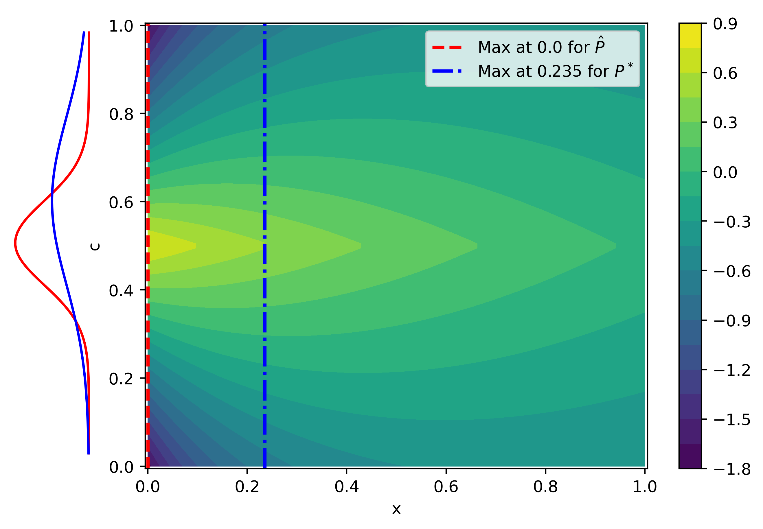
(a)

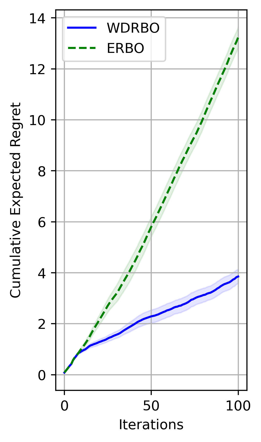
(b)

Figure 1: (a) Function $f(x,c)$ and its optima under optima under $\hat{\mathcal{P}}_{t}$ and $\mathcal{P}^{*}_{t}$. (b) Mean and standard error of the cumulative expected regret.

For the data-driven DRBO setting we adopt the setup of Huang et al. (2024) and provide a comparison of the different methods on synthetic function and the realistic problems. We will compare the algorithms’ performance based on the cumulative expected regret as in (11).

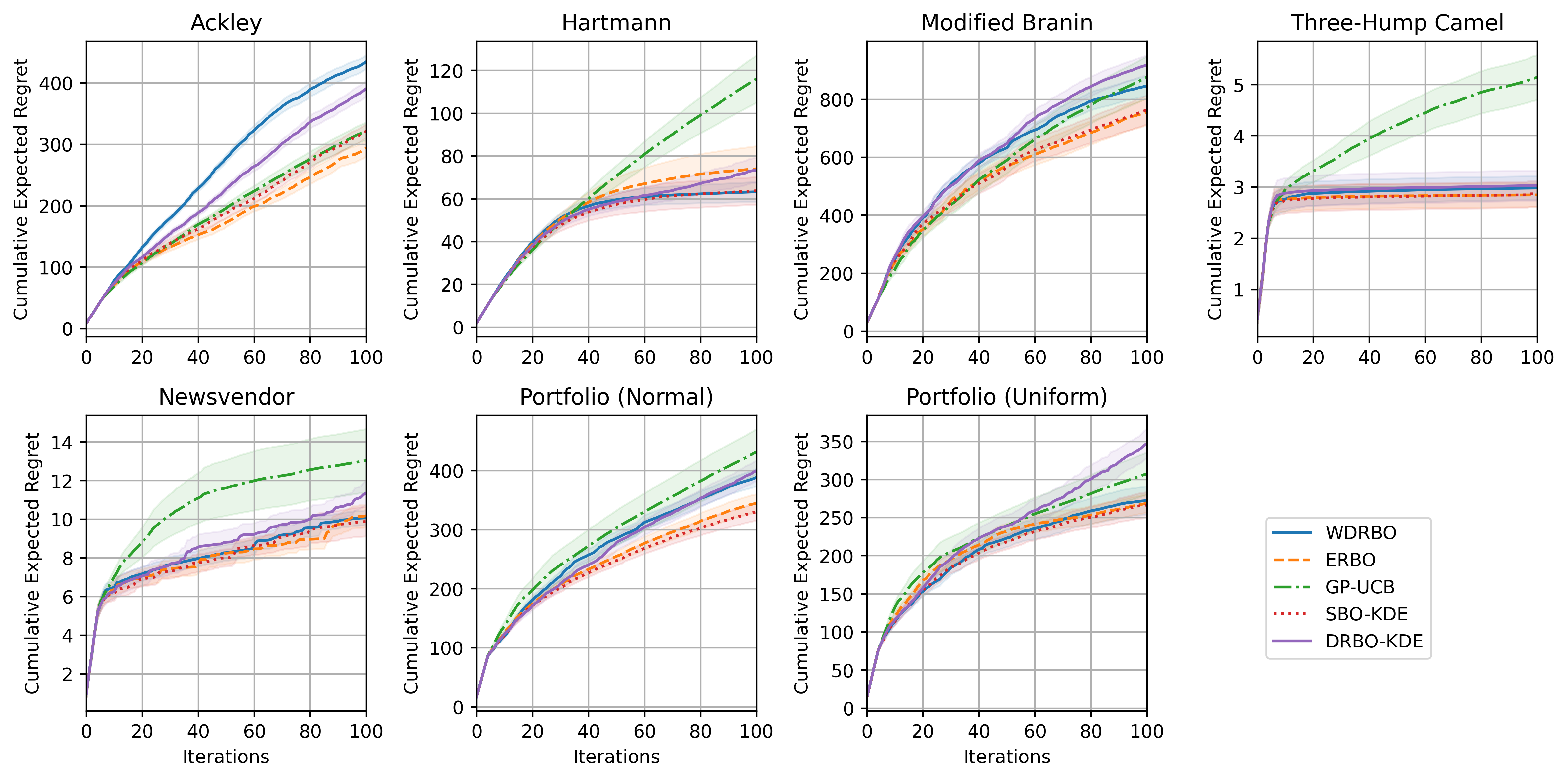
Figure 2: Mean and standard error of the cumulative expected regret.

We will compare compare the following algorithms: WDRBO: Data-Driven WDRBO algorithm with robustified acquisition function 13, where the center of the Wasserstein ambiguity set is given by the empirical distribution of the observed contexts and the radius is chosen as $\varepsilon_{t}=O(1/\sqrt{t})$.
ERBO: This is equivalent to WDRBO but we set $\varepsilon_{t}=0$ in the acquisition function 13, i.e. we maximize the empirical risk with respect to the observed contexts $x_{t}=\arg\max_{x\in\mathcal{X}}\mathbb{E}_{c\sim\hat{\mathcal{P}}_{t}}\left[\text{UCB}_{t}(x,c)\right]\$.
GP-UCB: Implements the UCB maximization algorithm proposed by Srinivas et al. (2012) ignoring the context variable in both the definition of the Gaussian process model and in the acquisition function maximization.
SBO-KDE: Stochastic BO formulation of Huang et al. (2024). An approximate context distribution is estimated from the observed samples by kernel density estimation. The acquisition function maximizes the expectation of the UCB with respect to the empirical distribution of the context obtained by sampling the approximate context distribution (sample average approximation).
DRBO-KDE: DR formulation of SBO-KDE proposed by Huang et al. (2024). Robustifies the SBO-KDE algorithm by considering DR formulation with a total variation ambiguity set. The ambiguity set is centered on the empirical distribution of the context obtained by sampling from the density estimate.
DRBO-MMD: DRBO formulation with MMD ambiguity set of Kirschner et al. (2020). The continuous context space is discretized and the UCB is maximized for the worst-case distribution supported on the discrete context space for a given MMD budget. The complexity of the robustified acquisition function scales with the cube of the cardinality of the context support.
DRBO-MMD Minmax: Minmax approximate formulation of DRBO-MMD proposed in Tay et al. (2022). The discretization can be finer as the worst-case sensitivity approximation reduces the computational burden of the method.
StableOpt: Implementation of StableOpt Bogunovic et al. (2018). Implements a robust acquisition function $x_{t}=\arg\max_{x\in\mathbb{X}}\min_{c\in C_{t}}\text{UCB}_{t}(x,c)$, where, following Huang et al. (2024), the set $C_{t}$ is chosen at each time $t$ as the set where for each dimension of the context we consider the interval $[\hat{\mu}_{t}^{c^{i}}-\hat{\sigma}_{t}^{c^{i}},\hat{\mu}_{t}^{c^{i}}+\hat{\sigma}_{t}^{c^{i}}]$, with $\hat{\mu}_{t}^{c^{i}}$ and $\hat{\sigma}_{t}^{c^{i}}$ the empirical mean and variance of the observed contexts.

For all the algorithms considered we fixed the value of the UCB trade-off parameter $\beta_{t}=1.5$. This has been done to be consistent with the engineering practice and earlier works such as Huang et al. (2024). We consider a set of artificial and real-world problems and different types of context distributions. For each problem and algorithm, we ran $100$ iterations and repeated over $15$ random seeds. Fig. 2 shows the resulting cumulative expected regret for WDRBO, ERBO, GP-UCB, SBO-KDE, and DRBO-KDE. More details about the specifics of the test problems and the implementations are left in the Appendix. We also leave the results for DRBO-MMD, DRBO-MMD Minmax, and StableOpt to the Appendix as their performance was not competitive with the other methods. The performance of DRBO-MMD is limited by the coarseness of the context discretization which is required to have a computationally tractable inner convex optimization step. The performance of DRBO-MMD Minmax is mainly limited by the worst-case sensitivity that introduces a linear term in the resulting regret bound. StableOpt suffers from the fact that it is solving a robust optimization problem.

We tracked the time required by each algorithm for a 100-iteration-long experiment. We report in Table 1 the computational times in seconds for the Ackley and Branin functions. The computational times are affected both by algorithm specific characteristics, e.g. an inner convex optimization problem is solved at each iteration, and by specific parameters choices, e.g. the discretization grid-size. The reported times have been obtained by running the algorithm on CPU only, as some of the algorithms have not been implemented to exploit the potential speed-ups resulting from running on GPU. For this test we used an Intel(R) Core(TM) i9-9900K@3.60GHz. GP-UCB has the smallest computational time as it ignores the context, thus also reducing the regression step complexity. ERBO and SBO-KDE are not robust approaches, the extra time required by SBO-KDE is due to the KDE step. One of the advantage of the proposed WDRBO is that is is able to add robustness against context distribution uncertainty without the large overheads of the other robust methods. The extra computational time required by WDRBO compared to ERBO is related to the calculation of the Lipschitz constant from the UCB expression. The main computational bottleneck for DRBO-MMD and DRBO-KDE is related to the solution of the inner minimization problems.

	Ackley	Branin
WDRBO (ours)	$44.3\pm 2.2$	$54.5\pm 2.6$
ERBO (ours)	$43.8\pm 1.6$	$45.2\pm 2.5$
GP-UCB	$15.7\pm 1.4$	$15.1\pm 1.0$
SBO-KDE	$46.7\pm 0.7$	$49.7\pm 1.5$
DRBO-KDE	$599.7\pm 33.0$	$525.0\pm 71.7$

Table 1: Mean and standard error of computational times in seconds for the Ackley ($d_{x}=1$, $d_{c}=1$) and Branin ($d_{x}=2$, $d_{c}=2$) functions.

We can see in Fig. 2 that the performance of WDRBO, ERBO, and SBO-KDE is extremely compelling, particularly when considering the computational complexity of the other algorithms. We argue that the performance of DRBO-KDE does not justify the extra computation required to solve the inner two-dimensional optimization problem. While we observe very strong performances for ERBO and SBO-KDE in the data-driven setting, with the smallest computational complexities, we want to highlight that, contrarily to WDRBO and DRBO-KDE, they do not compute a robust solution. This might lead to disappointing performance as shown in the first example where the ambiguity set does not collapse to the true distribution as the number of iterations grows, and for which a robust solution might be preferable.

6 CONCLUSIONS AND FUTURE WORK

In this paper, we introduced Wasserstein Distributionally Robust Bayesian Optimization (WDRBO), a novel algorithm that addresses the challenge of sequential data-driven decision-making under context distributional uncertainty. We developed a computationally tractable algorithm for WDRBO that can handle continuous context distributions, leveraging an approximate reformulation based on Lipschitz bounds of the acquisition function. This approach extends the existing literature on Distributionally Robust Bayesian Optimization by providing a principled method to handle continuous context distributions within a Wasserstein ambiguity set, allowing for a flexible and intuitive way to model uncertainty in the context distribution while maintaining computational feasibility.

Our theoretical analysis provides an cumulative expected regret bounds that match state-of-the-art results. Notably, for the data-driven setting, the bound does not require assumptions on the rate of decay of the ambiguity set radius but relies on finite-sample concentration results, making our approach more broadly applicable to real-world situations. Lastly, we conducted a comprehensive empirical evaluation demonstrating the effectiveness and practical applicability of WDRBO on both synthetic and real-world benchmarks. Our results show that the proposed WDRBO algorithm exhibits promising performance in terms of regret while avoiding computationally expensive inner optimization steps.

The promising results of WDRBO open up exciting opportunities for further research and development in the field of Distributionally Robust Bayesian optimization. Extending the WDRBO framework to risk measures, such as Conditional Value at Risk (CVaR), could broaden its applicability to risk-sensitive domains, such as robotics and finance.

Checklist

1. For all models and algorithms presented, check if you include:

   1. A clear description of the mathematical setting, assumptions, algorithm, and/or model. [Yes]

   2. An analysis of the properties and complexity (time, space, sample size) of any algorithm. [Yes]

   3. (Optional) Anonymized source code, with specification of all dependencies, including external libraries. [Yes]

2. For any theoretical claim, check if you include:

   1. Statements of the full set of assumptions of all theoretical results. [Yes]

   2. Complete proofs of all theoretical results. [Yes]

   3. Clear explanations of any assumptions. [Yes]

3. For all figures and tables that present empirical results, check if you include:

   1. The code, data, and instructions needed to reproduce the main experimental results (either in the supplemental material or as a URL). [Yes]

   2. All the training details (e.g., data splits, hyperparameters, how they were chosen). [Yes]

   3. A clear definition of the specific measure or statistics and error bars (e.g., with respect to the random seed after running experiments multiple times). [Yes]

   4. A description of the computing infrastructure used. (e.g., type of GPUs, internal cluster, or cloud provider). [Yes]

4. If you are using existing assets (e.g., code, data, models) or curating/releasing new assets, check if you include:

   1. Citations of the creator If your work uses existing assets. [Yes]

   2. The license information of the assets, if applicable. [Yes]

   3. New assets either in the supplemental material or as a URL, if applicable. [Yes]

   4. Information about consent from data providers/curators. [Not Applicable]

   5. Discussion of sensible content if applicable, e.g., personally identifiable information or offensive content. [Not Applicable]

5. If you used crowdsourcing or conducted research with human subjects, check if you include:

   1. The full text of instructions given to participants and screenshots. [Not Applicable]

   2. Descriptions of potential participant risks, with links to Institutional Review Board (IRB) approvals if applicable. [Not Applicable]

   3. The estimated hourly wage paid to participants and the total amount spent on participant compensation. [Not Applicable]

 

Wasserstein Distributionally Robust Bayesian Optimization with Continuous Context: Supplementary Materials

 

7 BACKGROUND ON RKHS AND KERNEL RIDGE REGRESSION

In this paper, we consider the frequentist perspective and formulate the surrogate model as the solution of a regularized least-squares regression problem in the Reproducing Kernel Hilbert Space (RKHS). A similar formulation can be derived following the Bayesian perspective of Gaussian Process Regression under suitable assumptions on the Gaussian Process prior and observation noise Kanagawa et al. (2018).

Consider an RKHS $({\mathcal{H}_{k}},\langle\cdot,\cdot\rangle_{\mathcal{H}_{k}})$ with reproducing kernel $k:\mathcal{Z}\times\mathcal{Z}\rightarrow\mathbb{R}$. Define the inner product of the RKHS as $f^{\top}g=\langle f,g\rangle_{\mathcal{H}_{k}}$ and the outer product as $fg^{\top}=f\langle g,\cdot\rangle_{\mathcal{H}_{k}}$. Let $\Phi_{t}:=(k(\cdot,z_{1}),\ldots,k(\cdot,z_{t}))^{\top}$ be the feature map of the RKHS for a sequence of points $z_{1},\ldots,z_{t}\in\mathcal{Z}$. Define the kernel matrix $K_{t}=\Phi_{t}\Phi_{t}^{\top}$ and the covariance operator $V_{t}=\Phi_{t}^{\top}\Phi_{t}$. The RKHS norm of a function $f\in{\mathcal{H}_{k}}$ is defined as $\|f\|_{\mathcal{H}_{k}}=\sqrt{f^{\top}f}=\sqrt{\langle f,f\rangle_{\mathcal{H}_{k}}}$. By the reproducing property of the kernel, we have that $f(z)=\langle f,k(\cdot,z)\rangle_{\mathcal{H}_{k}}$ for all $z\in\mathcal{Z}$.

With a slight abuse of notation we write the following equality which will be useful in the upcoming derivations

$$\lambda(\Phi_{t}^{\top}\Phi_{t}+\lambda I)^{-1}=I-\Phi_{t}^{\top}(\Phi_{t}\Phi_{t}^{\top}+\lambda I)^{-1}\Phi_{t}\ ,$$ (20)

where it should be clear from the context that $I$ is either the identity matrix or the identity operator in the RKHS. We also define the short-hand notation $\bar{V}_{t}=V_{t}+\lambda I=\Phi_{t}^{\top}\Phi_{t}+\lambda I$.

Given the observed data $\mathcal{D}_{t}=\{(z_{i},y_{i})\}_{i=1}^{t}$, the regularized least-squares regression problem in RKHS is defined as follows:

$$\min_{\mu\in{\mathcal{H}_{k}}}\sum_{i=1}^{t}(y_{i}-\mu(z_{i}))^{2}+\lambda\|\mu\|_{\mathcal{H}_{k}}^{2}.$$ (21)

The solution to this problem is given by:

$$\mu_{t} =\bar{V}_{t}^{-1}\Phi_{t}^{\top}y_{1:t}$$ (22)

$$=(V_{t}+\lambda I)^{-1}\Phi_{t}^{\top}y_{1:t}$$

$$=\Phi_{t}^{\top}(\Phi_{t}\Phi_{t}^{\top}+\lambda I)^{-1}y_{1:t}$$

where $y_{1:t}=(y_{1},\ldots,y_{t})^{\top}$ is the vector of observed responses. By the representation theorem, we can compute $\mu_{t}$ at some new point $z\in\mathcal{Z}$ as follows:

$$\mu_{t}(z) =\langle\mu_{t},k(\cdot,z)\rangle_{\mathcal{H}_{k}}$$ (23)

$$=\Phi_{t}^{\top}(\Phi_{t}\Phi_{t}^{\top}+\lambda I)^{-1}y_{1:t}$$

$$=k_{t}(z)^{\top}(K_{t}+\lambda I)^{-1}y_{1:t},$$

where $k_{t}(z)=(k(z,z_{1}),\ldots,k(z,z_{t}))^{\top}$ is the vector of kernel evaluations at $z$.

We can also compute

$$\sigma_{t}^{2}(z) :=\|k(\cdot,z)\|_{\bar{V}_{t}^{-1}}^{2}$$ (24)

$$=\frac{1}{\lambda}\left(k(z,z)-k_{t}(z)^{\top}(K_{t}+\lambda I)^{-1}k_{t}(z)\right),$$

where $\|k(\cdot,z)\|_{\bar{V}_{t}^{-1}}^{2}=k_{t}(z)^{\top}(\Phi_{t}^{\top}\Phi_{t}+\lambda I)^{-1}k_{t}(z)$, and we use (20) to get the final equation.

We are using the notation $\mu_{t}(z)$ and $\sigma_{t}^{2}(z)$ to align with the Gaussian Process Regression literature Kanagawa et al. (2018), where $\mu_{t}(z)$ and $\sigma_{t}^{2}(z)$ would represent the mean and variance of the Gaussian Process posterior at $z$ respectively.

7.1 Kernels that satisfy the Lipschitz condition in Assumption 1

Assumption 1 is satisfied for commonly used kernels. For example, it is satisfied with $L=1$ for the squared exponential kernel and the Matérn kernel for $\nu=3/2$ (Van Waarde and Sepulchre, 2022, Proposition 2). In fact, all smooth, positive definite, stationary kernels that have zero derivatives at zero satisfy Assumption 1. This, in turn, implies that Assumption 1 is satisfied for Matérn kernels with $\nu=p+1/2$, for $p=1,2,\dots$.

Lemma 11.

Let $k$ be a positive definite, stationary kernel such that $k(x,x^{\prime})=r(\|x-x^{\prime}\|)$, for some function $r:\mathbb{R}\to\mathbb{R}$ that is continuously twice differentiable in a neighborhood of the origin with first derivative $r^{(1)}(0)=0$. Then, the kernel-induced distance

$$d(x,x^{\prime}):=\sqrt{k(x,x)+k(x^{\prime},x^{\prime})-k(x,x^{\prime})-k(x^{\prime},x)}\leq M\|x-x^{\prime}\|,$$

for some constant $M>0$.

Proof.

Replacing $k$ with $r$ in the expression of $d(x,x^{\prime})$ we write

$$d(x,x^{\prime})=\sqrt{2r(0)-2r(\|x-x^{\prime}\|)}.$$

Pick any $\epsilon>0$. Let’s consider two cases:

Case 1: For $\|x-x^{\prime}\|\geq\epsilon$, by the positive definite property, we have $|r(\|x-x^{\prime}\|)|\leq r(0)$ for any $x,x^{\prime}$. Therefore:

$$d(x,x^{\prime})\leq 2\sqrt{r(0)}\leq 2\sqrt{r(0)}\,\|x-x^{\prime}\|/\epsilon=M_{1}\|x-x^{\prime}\|,$$

where $M_{1}=2\sqrt{r(0)}/\epsilon$.

Case 2: For $\|x-x^{\prime}\|\leq\epsilon$, using the Taylor remainder formula and the fact that $r^{(1)}(0)=0$:

$$r(\|x-x^{\prime}\|)=r(0)+\frac{\|x-x^{\prime}\|^{2}}{2}r^{(2)}(s),$$

for some $s\in[0,\|x-x^{\prime}\|]$. Since $r(\|x-x^{\prime}\|)\leq r(0)$, we have $\|x-x^{\prime}\|^{2}r^{(2)}(s)\leq 0$, which, in turn, implies that $r^{(2)}(s)\leq 0$. As a result,

$$d(x,x^{\prime})=\sqrt{-\|x-x^{\prime}\|^{2}r^{(2)}(s)}=\|x-x^{\prime}\|\sqrt{-r^{(2)}(s)}\leq\|x-x^{\prime}\|\max_{s\in[0,\epsilon]}\sqrt{-r^{(2)}(s)}=M_{2}\|x-x^{\prime}\|.$$

Since the function has a continuous second derivative in the interval $[0,\epsilon]$ and $r^{(2)}(s)\leq 0$ for all $s\in[0,\epsilon]$, the maximum $M_{2}=\max_{s\in[0,\epsilon]}\sqrt{-r^{(2)}(s)}$ is well-defined and finite.

The result follows by taking

$$M=\max\{M_{1},M_{2}\}=\max\left\{\frac{2\sqrt{r(0)}}{\epsilon},\max_{s\in[0,\epsilon]}\sqrt{-r^{(2)}(s)}\right\}$$

∎

8 MAIN PROOFS

We can state here a well-known result from the Wasserstein DR optimization literature Kuhn et al. (2019); Gao et al. (2024).

Lemma 12.

Consider a function $g:{\Xi}\rightarrow\mathbb{R}$ that is $L^{g}$-Lipschitz, i.e. $|g(\xi)-g(\xi^{\prime})|\leq L^{g}\|\xi-\xi^{\prime}\|$, for all $\xi,\xi^{\prime}\in{\Xi}$. Let $\mathcal{B}^{\varepsilon}(\hat{\mathcal{P}})$ be a Wasserstein ambiguity set defined as a ball of radius $\varepsilon$ in the Wasserstein distance centered at the distribution $\hat{\mathcal{P}}$. Then,

$$\sup_{\mathcal{Q}\in\mathcal{B}^{\varepsilon}(\hat{\mathcal{P}})}\mathbb{E}_{\xi\sim\mathcal{Q}}[g(\xi)]\leq\mathbb{E}_{\xi\sim\hat{\mathcal{P}}}[g(\xi)]+\varepsilon L^{g}\ ,$$ (25)

Similarly,

$$\inf_{\mathcal{Q}\in\mathcal{B}^{\varepsilon}(\hat{\mathcal{P}})}\mathbb{E}_{\xi\sim\mathcal{Q}}[g(\xi)]\geq\mathbb{E}_{\xi\sim\hat{\mathcal{P}}}[g(\xi)]-\varepsilon L^{g}\ .$$ (26)

As a consequence of Lemma 12, we can state the following result.

Lemma 13.

Let $f:\mathcal{X}\times\mathcal{C}\rightarrow\mathbb{R}$ be a function that is $L^{f}_{c}(x)$-Lipschitz in the context space, i.e. $|f(x,c)-f(x,c^{\prime})|\leq L^{f}_{c}(x)\|c-c^{\prime}\|$, for all $c,c^{\prime}\in\mathcal{C}$. Let $\mathcal{B}^{\varepsilon}(\hat{\mathcal{P}})$ be a Wasserstein ambiguity set defined as a ball of radius $\varepsilon$ in the Wasserstein distance centered at the distribution $\hat{\mathcal{P}}$. Then, for any $x\in\mathcal{X}$ and for any distribution $\tilde{\mathcal{P}}\in\mathcal{B}^{\varepsilon}(\hat{\mathcal{P}})$, we have that

$$|\mathbb{E}_{c\sim\tilde{\mathcal{P}}}[f(x,c)]-\mathbb{E}_{c\sim\hat{\mathcal{P}}}[f(x,c)]|\leq\varepsilon L^{f}_{c}(x)\ .$$ (27)

In order to provide rates for the cumulative expected regret we want to provide high probability bounds for the Lipschitz constants $L^{\text{UCB}_{t}}(x)$.

Lemma 14 (Lemma 3 in the main text).

Let $0<\delta<1$ be a failure probability and let

$$\bar{B}_{t}:=\lambda^{-\frac{1}{2}}R\sqrt{2\log\left(\frac{\det(I+\lambda^{-1}K_{t-1})^{\frac{1}{2}}}{\delta}\right)}+B\leq\lambda^{-\frac{1}{2}}\left(\left(R\sqrt{2\log\frac{1}{\delta}}+R\sqrt{2\gamma_{t}}\right)+B\right).$$ (28)

Then, with probability $1-\delta$ for all $t\geq 1$ we have $\|\mu_{t-1}\|_{\mathcal{H}_{k}}\leq\bar{B}_{t}.$ Further, if Assumption 1 holds (i.e., $\|k(\cdot,z)-k(\cdot,z^{\prime})\|_{\mathcal{H}_{k}}\leq L\|z-z^{\prime}\|$), we have:

(i) With probability $1-\delta$, for any $z,z^{\prime}\in\mathcal{X}\times\mathcal{C}$: $|\mu_{t-1}(z)-\mu_{t-1}(z^{\prime})|\leq\bar{B}_{t}L\|z-z^{\prime}\|.$

(ii) For any $z,z^{\prime}\in\mathcal{X}\times\mathcal{C}$: $|\beta_{t}\sigma_{t-1}(z)-\beta_{t}\sigma_{t-1}(z^{\prime})|\leq\beta_{t}\lambda^{-\frac{1}{2}}L\|z-z^{\prime}\|=\bar{B}_{t}L\|z-z^{\prime}\|.$

Therefore, with probability $1-\delta$, the UCB function is Lipschitz continuous with constant: $L^{\text{UCB}_{t}}\leq 2\bar{B}_{t}L.$

Proof.

The UCB is defined as:

$$\text{UCB}_{t}(z)=\mu_{t-1}(z)+\beta_{t}\sigma_{t-1}(z),$$

where $z=(x,c)\in\mathcal{X}\times\mathcal{C}$.

We have

$$\mu_{t}(z)=\langle(\lambda I+V_{t})^{-1}\Phi_{t}^{\top}y_{1:t},k(\cdot,z)\rangle,$$ (29)

and

$$\|\mu_{t}\|_{\mathcal{H}_{k}} =\|(\lambda I+V_{t})^{-1}\Phi_{t}^{\top}y_{1:t}\|_{\mathcal{H}_{k}}$$ (30)

$$=\|(\lambda I+V_{t})^{-1}\Phi_{t}^{\top}(f(z_{1:t})+\eta_{1:t})\|_{\mathcal{H}_{k}}$$ (31)

$$=\|(\lambda I+V_{t})^{-1}\Phi_{t}^{\top}(\Phi_{t}f+\eta_{1:t})\|_{\mathcal{H}_{k}}$$ (32)

$$\leq\|(\lambda I+V_{t})^{-1}\Phi_{t}^{\top}\Phi_{t}f\|_{\mathcal{H}_{k}}+\|(\lambda I+V_{t})^{-1}\Phi_{t}^{\top}\eta_{1:t}\|_{\mathcal{H}_{k}}$$ (33)

$$=\|(\lambda I+V_{t})^{-1}V_{t}f\|_{\mathcal{H}_{k}}+\|(\lambda I+V_{t})^{-1}\Phi_{t}^{\top}\eta_{1:t}\|_{\mathcal{H}_{k}}$$ (34)

$$\leq\|(\lambda I+V_{t})^{-1}V_{t}\|_{\mathcal{H}_{k}}\|f\|_{\mathcal{H}_{k}}+\|(\lambda I+V_{t})^{-\frac{1}{2}}\|_{\mathcal{H}_{k}}\|(\lambda I+V_{t})^{-\frac{1}{2}}\Phi_{t}^{\top}\eta_{1:t}\|_{\mathcal{H}_{k}}$$ (35)

$$\leq B+\lambda^{-\frac{1}{2}}\|(\lambda I+V_{t})^{-\frac{1}{2}}\Phi_{t}^{\top}\eta_{1:t}\|_{\mathcal{H}_{k}},$$ (36)

where we used the assumption that $\|f\|_{\mathcal{H}_{k}}\leq B$ and the fact that $\|(\lambda I+V_{t})^{-1}V_{t}\|_{\mathcal{H}_{k}}\leq 1$ for $\lambda\geq 0$.

Applying Corollary 3.6 of Abbasi-Yadkori (2013), with probability at least $1-\delta$ and for all $t\geq 1$, we have

$$\|(\lambda I+V_{t})^{-\frac{1}{2}}\Phi_{t}^{\top}\eta_{1:t}\|_{\mathcal{H}_{k}}\leq R\sqrt{2\log\left(\frac{\det(I+\lambda^{-1}V_{t})^{\frac{1}{2}}}{\delta}\right)}=R\sqrt{2\log\left(\frac{\det(I+\lambda^{-1}K_{t})^{\frac{1}{2}}}{\delta}\right)}.$$ (37)

Thus, we obtain

$$\|\mu_{t}\|_{\mathcal{H}_{k}}\leq\lambda^{-\frac{1}{2}}R\sqrt{2\log\left(\frac{\det(I+\lambda^{-1}K_{t})^{\frac{1}{2}}}{\delta}\right)}+B=\bar{B}_{t}.$$ (38)

If Assumption 1 holds, for any $z,z^{\prime}\in\mathcal{X}\times\mathcal{C}$, we have:

$$|\mu_{t-1}(z)-\mu_{t-1}(z^{\prime})| =|\langle\mu_{t-1},k(\cdot,z)-k(\cdot,z^{\prime})\rangle_{\mathcal{H}_{k}}|$$ (39)

$$\leq\|\mu_{t-1}\|_{\mathcal{H}_{k}}\cdot\|k(\cdot,z)-k(\cdot,z^{\prime})\|_{\mathcal{H}_{k}}$$ (40)

$$\leq\bar{B}_{t}\cdot L\|z-z^{\prime}\|$$ (41)

where we used the Cauchy-Schwarz inequality and Assumption 1.

For the term $\beta_{t}\sigma_{t-1}(z)$, we need to analyze the Lipschitz property of $\sigma_{t-1}(z)$. We know by the Woodbury identity:

$$\sigma_{t-1}^{2}(z)=\langle k(\cdot,z),(\lambda I+V_{t-1})^{-1}k(\cdot,z)\rangle_{\mathcal{H}_{k}}=\frac{1}{\lambda}\left(k(z,z)-k_{t-1}(z)^{\top}(K_{t-1}+\lambda I)^{-1}k_{t-1}(z)\right)$$ (42)

This gives us:

$$\sigma_{t-1}(z)=\|(\lambda I+V_{t-1})^{-1/2}k(\cdot,z)\|_{\mathcal{H}_{k}}$$ (43)

Now, for the Lipschitz property, by the triangle inequality:

$$|\sigma_{t-1}(z)-\sigma_{t-1}(z^{\prime})| \leq\|(\lambda I+V_{t-1})^{-1/2}(k(\cdot,z)-k(\cdot,z^{\prime}))\|_{\mathcal{H}_{k}}$$ (44)

$$\leq\|(\lambda I+V_{t-1})^{-1/2}\|_{op}\cdot\|k(\cdot,z)-k(\cdot,z^{\prime})\|_{\mathcal{H}_{k}}$$ (45)

$$\leq\lambda^{-\frac{1}{2}}\cdot L\|z-z^{\prime}\|$$ (46)

where we used the fact that $\|(\lambda I+V_{t-1})^{-1/2}\|_{op}\leq\lambda^{-\frac{1}{2}}$ and Assumption 1.

Therefore:

$$|\beta_{t}\sigma_{t-1}(z)-\beta_{t}\sigma_{t-1}(z^{\prime})|\leq\beta_{t}\lambda^{-\frac{1}{2}}L\|z-z^{\prime}\|$$ (47)

Note that, recalling the definition of $\beta_{t}$:

$$\beta_{t}:=R\sqrt{2\log\left(\frac{\det(I+\lambda^{-1}K_{t-1})^{\frac{1}{2}}}{\delta}\right)}+\lambda^{\frac{1}{2}}B,$$ (48)

we can observe that $\beta_{t}\lambda^{-\frac{1}{2}}=\bar{B}_{t}$.

Combining the results, with probability $1-\delta$, we have:

$$|UCB(z)-UCB(z^{\prime})| =|\mu_{t-1}(z)+\beta_{t}\sigma_{t-1}(z)-\mu_{t-1}(z^{\prime})-\beta_{t}\sigma_{t-1}(z^{\prime})|$$ (49)

$$\leq|\mu_{t-1}(z)-\mu_{t-1}(z^{\prime})|+|\beta_{t}\sigma_{t-1}(z)-\beta_{t}\sigma_{t-1}(z^{\prime})|$$ (50)

$$\leq\bar{B}_{t}L\|z-z^{\prime}\|+\beta_{t}\lambda^{-\frac{1}{2}}L\|z-z^{\prime}\|$$ (51)

$$=(\bar{B}_{t}L+\bar{B}_{t}L)\|z-z^{\prime}\|$$ (52)

$$=2\bar{B}_{t}L\|z-z^{\prime}\|$$ (53)

where we used the fact that $\beta_{t}\lambda^{-\frac{1}{2}}=\bar{B}_{t}$.

Thus, with probability $1-\delta$, for all $x\in\mathcal{X}$ the Lipschitz constant of the UCB function with respect to the context is bounded by:

$$L^{\text{UCB}_{t}}(x)\leq 2\bar{B}_{t}L$$ (54)

which concludes the proof. ∎

Theorem 15 (Instantaneous expected regret - Thm. 4 in the main text).

Let Assumption 1 hold. Fix a failure probability $0<\delta<1$. With probability at least $1-\delta$, for all $t\geq 1$ the instantaneous expected regret can be bounded by

$$r_{t}\leq\mathbb{E}_{c\sim\mathcal{P}^{*}_{t}}\left[2\beta_{t}\sigma_{t-1}(x_{t},c)\right]+2\varepsilon_{t}L^{\text{UCB}_{t}}(x^{*}_{t})$$ (55)

Proof.

Recall that the benchmark solution $x^{*}_{t}$ is the optimal solution to the stochastic optimization problem at time-step $t$, given access to the true function $f$ and context distribution $\mathcal{P}^{*}_{t}$

$$x^{*}_{t}=\arg\max_{x\in\mathcal{X}}\mathbb{E}_{c\sim\mathcal{P}^{*}_{t}}{[f(x,c)]}\ .$$

Whereas $x_{t}$ is the solution to the robustified UCB acquisition function as given in (13)

$$x_{t}=\arg\max_{x\in\mathcal{X}}\mathbb{E}_{c\sim\hat{\mathcal{P}}_{t}}\left[\text{UCB}_{t}(x,c)\right]-\varepsilon_{t}L^{\text{UCB}_{t}}(x)\ ,$$

From the definition of instantaneous regret, we can write:

$$r_{t} =\mathbb{E}_{c\sim\mathcal{P}^{*}_{t}}{[f(x^{*}_{t},c)]}-\mathbb{E}_{c\sim\mathcal{P}^{*}_{t}}{[f(x_{t},c)]}$$ (56)

$$\overset{\textup{\makebox[0.0pt]{(i)}}\ltx@label{proof_{i}nst_{r}egret_{1}}}{\leq}\mathbb{E}_{c\sim\mathcal{P}^{*}_{t}}\left[\text{UCB}_{t}(x^{*}_{t},c)\right]-\mathbb{E}_{c\sim\mathcal{P}^{*}_{t}}\left[\text{LCB}_{t}(x_{t},c)\right]$$

$$\overset{\textup{\makebox[0.0pt]{(ii)}}\ltx@label{proof_{i}nst_{r}egret_{2}}}{\leq}\mathbb{E}_{c\sim\hat{\mathcal{P}}_{t}}\left[\text{UCB}_{t}(x^{*}_{t},c)\right]+\varepsilon_{t}L^{\text{UCB}_{t}}(x^{*}_{t})-\mathbb{E}_{c\sim\mathcal{P}^{*}_{t}}\left[\text{LCB}_{t}(x_{t},c)\right]$$

$$\overset{\textup{\makebox[0.0pt]{(iii)}}\ltx@label{proof_{i}nst_{r}egret_{3}}}{\leq}\mathbb{E}_{c\sim\hat{\mathcal{P}}_{t}}\left[\text{UCB}_{t}(x_{t},c)\right]-\varepsilon_{t}L^{\text{UCB}_{t}}(x_{t})+2\varepsilon_{t}L^{\text{UCB}_{t}}(x^{*}_{t})-\mathbb{E}_{c\sim\mathcal{P}^{*}_{t}}\left[\text{LCB}_{t}(x_{t},c)\right]$$

$$\overset{\textup{\makebox[0.0pt]{(iv)}}\ltx@label{proof_{i}nst_{r}egret_{4}}}{\leq}\mathbb{E}_{c\sim\mathcal{P}^{*}_{t}}\left[\text{UCB}_{t}(x_{t},c)\right]+2\varepsilon_{t}L^{\text{UCB}_{t}}(x^{*}_{t})-\mathbb{E}_{c\sim\mathcal{P}^{*}_{t}}\left[\text{LCB}_{t}(x_{t},c)\right]$$

$$\overset{\textup{\makebox[0.0pt]{(v)}}\ltx@label{proof_{i}nst_{r}egret_{5}}}{\leq}\mathbb{E}_{c\sim\mathcal{P}^{*}_{t}}[\mu_{t-1}(x_{t},c)+\beta_{t}\sigma_{t-1}(x_{t},c)-\mu_{t-1}(x_{t},c)+\beta_{t}\sigma_{t-1}(x_{t},c)]+2\varepsilon_{t}L^{\text{UCB}_{t}}(x^{*}_{t})$$

$$=\mathbb{E}_{c\sim\mathcal{P}^{*}_{t}}\left[2\beta_{t}\sigma_{t-1}(x_{t},c)\right]+2\varepsilon_{t}L^{\text{UCB}_{t}}(x^{*}_{t})\ .$$

Where LABEL:proof_inst_regret_1 holds with probability $1-\delta$ by definition of UCB and LCB, with $\beta_{t}$ chosen as in Lemma 1. LABEL:proof_inst_regret_2 holds by applying Lemma 2 under the assumption that $\mathcal{P}^{*}_{t}\in\mathcal{B}^{\varepsilon_{t}}(\hat{\mathcal{P}}_{t})$. In LABEL:proof_inst_regret_3 we add and subtract $\varepsilon_{t}L^{\text{UCB}_{t}}(x^{*})$ and use the fact that $x_{t}$ is the maximizer of the acquisition function (13). The inequality LABEL:proof_inst_regret_4 follows from another application of Lemma 2, and finally LABEL:proof_inst_regret_5 follows again from the definitions of the UCB and the LCB. ∎

Theorem 16 (cumulative expected regret - Thm. 5 in the main text).

Let Assumption 1 hold. Fix a failure probability $0<\delta<1$. With probability at least $1-2\delta$, the cumulative expected regret after $T$ steps can be bounded as:

$$R_{T}\leq 4\beta_{T}\sqrt{T\left(\gamma_{T}+4\log\frac{6}{\delta}\right)}+\sum_{t=1}^{T}\varepsilon_{t}2L^{\text{UCB}_{t}}(x^{*}_{t})\ ,$$ (57)

where $\gamma_{T}$ is the maximum information gain (Srinivas et al., 2009; Chowdhury and Gopalan, 2017; Vakili et al., 2021) at time $T$, which is defined as

$$\gamma_{t}:=\sup_{z_{1},z_{2},\dots,z_{t}}\log\det\left(I+\lambda^{-1}K_{t-1}\right)\ .$$

Proof.

Starting from the definition of cumulative expected regret:

$$R_{T} =\sum_{t=1}^{T}r_{t}=\sum_{t=1}^{T}\mathbb{E}_{c\sim\mathcal{P}^{*}_{t}}{[f(x^{*}_{t},c)]}-\mathbb{E}_{c\sim\mathcal{P}^{*}_{t}}{[f(x_{t},c)]}$$ (58)

$$\overset{\textup{\makebox[0.0pt]{(i)}}\ltx@label{proof_{c}um_{r}egret_{1}}}{\leq}\sum_{t=1}^{T}\mathbb{E}_{c\sim\mathcal{P}^{*}_{t}}\left[2\beta_{t}\sigma_{t-1}(x_{t},c)\right]+\sum_{t=1}^{T}\varepsilon_{t}2L^{\text{UCB}_{t}}(x^{*}_{t})$$

$$\leq 2\beta_{T}\sum_{t=1}^{T}\mathbb{E}_{c\sim\mathcal{P}^{*}_{t}}\left[\sigma_{t-1}(x_{t},c)\right]+\sum_{t=1}^{T}\varepsilon_{t}2L^{\text{UCB}_{t}}(x^{*}_{t})$$

$$\overset{\textup{\makebox[0.0pt]{(ii)}}\ltx@label{proof_{c}um_{r}egret_{2}}}{\leq}2\beta_{T}\sqrt{T\sum_{t=1}^{T}\left(\mathbb{E}_{c\sim\mathcal{P}^{*}_{t}}\left[\sigma_{t-1}(x_{t},c)\right]\right)^{2}}+\sum_{t=1}^{T}\varepsilon_{t}2L^{\text{UCB}_{t}}(x^{*}_{t})$$

$$\overset{\textup{\makebox[0.0pt]{(iii)}}\ltx@label{proof_{c}um_{r}egret_{3}}}{\leq}2\beta_{T}\sqrt{T\sum_{t=1}^{T}\mathbb{E}_{c\sim\mathcal{P}^{*}_{t}}\left[\sigma_{t-1}(x_{t},c)^{2}\right]}+\sum_{t=1}^{T}\varepsilon_{t}2L^{\text{UCB}_{t}}(x^{*}_{t})$$

Where the inequality LABEL:proof_cum_regret_1 follows from Theorem 15, LABEL:proof_cum_regret_2 follows from the Cauchy-Schwarz inequality, and LABEL:proof_cum_regret_3 follows from Jensen’s inequality.

We can now apply the concentration of conditional mean result from Lemma 7 of Kirschner et al. (2020) (see also Lemma 3 of Kirschner and Krause (2018)), with probability at least $1-\delta$ we obtain for all $T$:

$$\sum_{t=1}^{T}\mathbb{E}_{c\sim\mathcal{P}^{*}_{t}}\left[\sigma_{t-1}(x_{t},c)^{2}\right]$$ (59)

$$\overset{\textup{\makebox[0.0pt]{(i)}}\ltx@label{proof_{c}cmean_{1}}}{\leq}\ 2\sum_{t=1}^{T}\sigma_{t-1}(x_{t},c_{t})^{2}+8\log\frac{6}{\delta}$$

$$\overset{\textup{\makebox[0.0pt]{(ii)}}\ltx@label{proof_{c}cmean_{2}}}{\leq}\ 2\sum_{t=1}^{T}2\log(1+\sigma_{t-1}(x_{t},c_{t})^{2})+8\log\frac{6}{\delta}$$

$$\overset{\textup{\makebox[0.0pt]{(iii)}}\ltx@label{proof_{c}cmean_{3}}}{\leq}\ 4\gamma_{T}+16\log\frac{6}{\delta}$$

where LABEL:proof_ccmean_1 follows from Lemma 7 of  Kirschner et al. (2020) noting that $k(z,z^{\prime})\leq 1$ by assumption, LABEL:proof_ccmean_2 follows from the fact that $x\leq 2a\log(1+x)$ for all $x\in[0,a]$, and LABEL:proof_ccmean_3 follows from the definition of maximum information gain. By substituting this result into the cumulative regret expression we get with probability $1-2\delta$:

$$R_{T}\leq \ 4\beta_{t}\sqrt{T\left(\gamma_{T}+4\log\frac{6}{\delta}\right)}+\sum_{t=1}^{T}\varepsilon_{t}2L^{\text{UCB}_{t}}(x^{*}_{t})\ ,$$ (60)

which concludes the proof. ∎

Corollary 17 (Corollary 6 in the main text – General WDRBO Regret Order).

Let $0<\delta<1$ be a failure probability and let Assumption 1 hold. Then, with probability $1-2\delta$, the cumulative expected regret is of the order of

$$R_{T}=\tilde{O}\left(\sqrt{T}\gamma_{T}+\sqrt{\gamma_{T}}\sum_{t=1}^{T}\varepsilon_{t}\right)\ .$$

For the Squared Exponential kernel, this reduces to

$$R_{T}=\tilde{O}\left(\sqrt{T}+\sum_{t=1}^{T}\varepsilon_{t}\right)\ ,$$

where $\tilde{O}$ omits logarithmic terms.

Proof.

We can combine the results of Theorem 5 and Lemma 6 to write

$$R_{T}\leq \ 4\beta_{t}\sqrt{T\gamma_{T}+4\log\frac{6}{\delta}}+\sum_{t=1}^{T}\varepsilon_{t}2L^{\text{UCB}_{t}}(x^{*}_{t})$$ (61)

$$\leq \ 4\beta_{t}\sqrt{T\gamma_{T}+4\log\frac{6}{\delta}}+\sum_{t=1}^{T}\varepsilon_{t}4\lambda^{-\frac{1}{2}}\left(\left(R\sqrt{2\log\frac{1}{\delta}}+R\sqrt{2\gamma_{t}}\right)+B\right)L$$

$$\leq \ 4(R\sqrt{2\log(1/\delta)}+R\sqrt{2\gamma_{T}}+\lambda^{\frac{1}{2}}B)\sqrt{T\gamma_{T}+4\log\frac{6}{\delta}}+\sum_{t=1}^{T}\varepsilon_{t}4\lambda^{-\frac{1}{2}}\left(\left(R\sqrt{2\log\frac{1}{\delta}}+R\sqrt{2\gamma_{t}}\right)+B\right)L$$

$$= \ \mathcal{O}(\gamma_{T}\sqrt{T}+\sqrt{\lambda\gamma_{T}T})+\sum_{t=1}^{T}\varepsilon_{t}\mathcal{O}(\lambda^{-\frac{1}{2}}\sqrt{\gamma_{T}})$$

$$= \ \mathcal{O}(\gamma_{T}\sqrt{T}+\lambda^{-\frac{1}{2}}\sqrt{\gamma_{T}}\sum_{t=1}^{T}\varepsilon_{t})\ ,$$

which proves the first statement.

The maximum information gain for the Squared Exponential kernel can be bounded as Vakili et al. (2021):

$$\gamma_{t}\leq\mathcal{O}(\log^{d+1}(t))\ .$$

Thus, the rate for the cumulative expected regret is

$$R_{T}=\tilde{\mathcal{O}}\left(\sqrt{T}+\sum_{t=1}^{T}\varepsilon_{t}\right)$$

∎

8.1 Proofs of the data-driven setting

We can now show how this result translates to the data-driven formulation, and provide a rate for the cumulative expected regret.

Define the class of functions

$$\mathcal{U}(m,b,s)=\left\{h:h(z)=\mu(z)+\beta\sigma(z)\ ,\ \|\mu\|_{\mathcal{H}_{k}}\leq m,\ \beta\leq b,\ \sigma(z)\in{\bm{\sigma}}_{s}\right\}\ ,$$

where ${\bm{\sigma}}_{s}=\left\{\sigma:\sigma(z)=\|\mathcal{M}k(\cdot,z)\|_{\mathcal{H}_{k}}\text{ with }\|\mathcal{M}\|_{op}\leq s^{-\frac{1}{2}}\right\}\ .$ Following this definition, the set $\mathcal{U}(\bar{B}_{t},\bar{B}_{t},\lambda)$ contains the UCB functions in the form of (9), which follows from the definitions of $\mu_{t}$, $\sigma_{t}$, and $\beta_{t}$ given in (4), (5), (7) respectively. The RKHS-norm bound on $\mu_{t-1}$ follows from (38), the bound on $\beta_{t}$ follows from Lemma 1, and the condition $\sigma_{t-1}(z)\in{\bm{\sigma}}^{\lambda}$ follows from the fact that the minimum singular value of $\lambda I+V_{t-1}$ is larger than $\lambda$. Let $\mathcal{N}_{\infty}(\rho,\mathcal{U}(m,b,s))$ be the $\rho$-covering number with respect to the $\infty$-norm of the set $\mathcal{U}(m,b,s)$.

The following result is an adaptation of Corollary 2 of Gao (2023). Let ${\mathrm{D}_{\mathcal{X}}}$, ${\mathrm{D}_{\mathcal{C}}}$ denote the diameters of the sets $\mathcal{X},\mathcal{C}$ respectively.

Lemma 18.

Let $0<\delta<1$ be a failure probability. Let

$$\varepsilon_{t}(\rho)=\sqrt{2{\mathrm{D}_{\mathcal{C}}}^{2}\frac{\log 1/\delta+d_{x}\log(1+2\rho^{-1}{\mathrm{D}_{\mathcal{X}}})+\log\mathcal{N}_{\infty}(\rho,\mathcal{U}(m,b,s))}{t}}.$$

With probability at least $1-\delta$

$$\forall h\in\mathcal{U}(m,b,s),\forall x\in\mathcal{X}:\quad\mathbb{E}_{c\sim\mathcal{P}^{*}}[h(x,c)]\leq\mathbb{E}_{c\sim\hat{\mathcal{P}}_{t}}[h(x,c)]+\varepsilon_{t}(\rho)L^{h}_{c}(x)+(1+L_{x})\rho.$$ (62)

where $L^{h}_{c}(x)$ denotes the Lipschitz constant of function $h(x,\cdot)$ with respect to the context $c$, and $L_{x}$ is such that $\forall\ h\ \in\mathcal{U}(m,b,s),\ x,\ \tilde{x}\ \in\mathcal{X},\ c\in\mathcal{C}$ we have that $|h(x,c)-{h}(\tilde{x},c)|\leq L_{x}\|x-\tilde{x}\|$.

Proof.

Let $h\in\mathcal{U}(m,b,s)$, $x\in\mathcal{X}$. Following the notation of Gao (2023), let for any $\varepsilon>0$

$$\mathcal{R}_{\mathcal{P}}(\varepsilon,h(x,\cdot))=\sup_{\mathcal{Q}\in\mathcal{B}^{\varepsilon}(\mathcal{P})}\mathbb{E}_{c\sim\mathcal{Q}}(h(x,c))-\mathbb{E}_{c\sim\mathcal{P}}(h(x,c)).$$

Using the Lipschitz bound from Lemma 3, it holds that

$$\mathcal{R}_{\mathcal{P}}(\varepsilon,h(x,\cdot))\leq\varepsilon L^{h}_{c}(x)$$ (63)

Let $\tilde{h}\in\mathcal{U}(m,b,s),\,\tilde{x}\in\mathcal{X}$. Following the proof of Corollary 2 in Gao (2023), we have

$$\mathcal{R}_{\mathcal{P}}(\varepsilon,-h(x,\cdot))-\mathcal{R}_{\mathcal{P}}(\varepsilon,-\tilde{h}(\tilde{x},\cdot))\leq\sup_{\mathcal{Q}\in\mathcal{B}^{\varepsilon}(\mathcal{P})}|\mathbb{E}_{c\sim\mathcal{Q}}(\tilde{h}(\tilde{x},c))-\mathbb{E}_{c\sim\mathcal{Q}}(h(x,c))|.$$

Using the decomposition

$$|h(x,c)-\tilde{h}(\tilde{x},c)| =|h(x,c)-\tilde{h}(x,c)+\tilde{h}(x,c)-\tilde{h}(\tilde{x},c)|$$

$$\leq\|h-\tilde{h}\|_{\infty}+L_{x}\|x-\tilde{x}\|,$$

we obtain

$$\mathcal{R}_{\mathcal{P}}(\varepsilon,-h(x,\cdot))-\mathcal{R}_{\mathcal{P}}(\varepsilon,-\tilde{h}(\tilde{x},\cdot))\leq\|h-\tilde{h}\|_{\infty}+L_{x}\|x-\tilde{x}\|$$ (64)

Similarly

$$|\mathbb{E}_{c\sim\mathcal{P}^{*}}(\tilde{h}(\tilde{x},c))-\mathbb{E}_{c\sim\mathcal{P}^{*}}(h(x,c))| \leq\|h-\tilde{h}\|_{\infty}+L_{x}\|x-\tilde{x}\|$$ (65)

$$|\mathbb{E}_{c\sim\hat{\mathcal{P}}_{t}}(\tilde{h}(\tilde{x},c))-\mathbb{E}_{c\sim\hat{\mathcal{P}}_{t}}(h(x,c))| \leq\|h-\tilde{h}\|_{\infty}+L_{x}\|x-\tilde{x}\|$$

Let $\mathcal{X}_{\rho}$ be a covering of $\mathcal{X}$ of precision $\rho$ with respect to the Euclidean norm and $\mathcal{U}_{\rho}(m,b,s)$ be a covering of $\mathcal{U}(m,b,s)$ of precision $\rho$ with respect to the infinity norm. We have that $|\mathcal{X}_{\rho}|\leq(1+2{\mathrm{D}_{\mathcal{X}}}\rho^{-1})^{{d_{x}}}$ (Vershynin, 2018, Ch. 4), while by definition $|\mathcal{U}_{\rho}(m,b,s)|=\mathcal{N}_{\infty}(\rho,\mathcal{U}(m,b,s))$.

By the definition of the coverings and (64), (65), we have that

$$\forall\tilde{h}\in\mathcal{U}_{\rho}(m,b,s),\forall\tilde{x}\in\mathcal{X}_{\rho}\quad \mathbb{E}_{c\sim\mathcal{P}^{*}}[\tilde{h}(\tilde{x},c)] \leq\mathbb{E}_{c\sim\hat{\mathcal{P}}_{t}}[\tilde{h}(\tilde{x},c)]+\mathcal{R}_{\mathcal{\mathcal{P}^{*}}}(\varepsilon,\tilde{h}(\tilde{x},\cdot))\Rightarrow$$

$$\forall h\in\mathcal{U}(m,b,s),\forall x\in\mathcal{X}\quad \mathbb{E}_{c\sim\mathcal{P}^{*}}[h(x,c)] \leq\mathbb{E}_{c\sim\hat{\mathcal{P}}_{t}}[h(x,c)]+\mathcal{R}_{\mathcal{\mathcal{P}^{*}}}(\varepsilon,h(x,\cdot))+\min_{\tilde{h}\in\mathcal{U}_{\rho,t}}\|h-\tilde{h}\|_{\infty}+L_{x}\min_{\tilde{x}\in\mathcal{X}_{\rho}}\|x-\tilde{x}\|$$

$$\leq\mathbb{E}_{c\sim\hat{\mathcal{P}}_{t}}[h(x,c)]+\mathcal{R}_{\mathcal{\mathcal{P}^{*}}}(\varepsilon,h(x,\cdot))+L_{x}\rho.$$

Hence,

$$\mathbb{P}(\forall h\in\mathcal{U}(m,b,s),\forall x\in\mathcal{X}:\quad\mathbb{E}_{c\sim\mathcal{P}^{*}}[h(x,c)]\leq\mathbb{E}_{c\sim\hat{\mathcal{P}}_{t}}[h(x,c)]+\mathcal{R}_{\mathcal{\mathcal{P}^{*}}}(\varepsilon,h(x,\cdot))+(1+L_{x})\rho)$$

$$\geq 1-\sum_{\tilde{h}\in\mathcal{U}_{\rho,t}}\sum_{\tilde{x}\in\mathcal{X}_{\rho}}\mathbb{P}(\mathbb{E}_{c\sim\mathcal{P}^{*}}[\tilde{h}(\tilde{x},c)]\geq\mathbb{E}_{c\sim\hat{\mathcal{P}}_{t}}[\tilde{h}(\tilde{x},c)]+\mathcal{R}_{\mathcal{\mathcal{P}^{*}}}(\varepsilon,\tilde{h}(\tilde{x},\cdot)))$$

$$\geq 1-|\mathcal{X}_{\rho}||\mathcal{U}_{\rho}(m,b,s)|e^{-\varepsilon^{2}\frac{t}{2{\mathrm{D}_{\mathcal{C}}}^{2}}},$$

where the last inequality follows from Theorem 1 in Gao (2023). The result follows from picking $\varepsilon=\varepsilon_{t}(\rho)$. ∎

Lemma 19.

Let $0<\delta<1$ be a failure probability, and let $h\in\mathcal{U}(m,b,s)$. Let

$$\varepsilon_{t}(\rho)=\sqrt{2{\mathrm{D}_{\mathcal{C}}}^{2}\frac{\log 1/\delta+d_{x}\log(1+2\rho^{-1}{\mathrm{D}_{\mathcal{X}}})+\log\mathcal{N}_{\infty}(\rho,\mathcal{U}(m,b,s))}{t}}.$$

Then, with probability at least $1-\delta$, and for any $x\in\mathcal{X}$, we have that

$$|\mathbb{E}_{c\sim\mathcal{P}^{*}}[h(x,c)]-\mathbb{E}_{c\sim\hat{\mathcal{P}}_{t}}[h(x,c)]|\leq\varepsilon_{t}(\rho)L^{h}_{c}(x)+(1+L_{x})\rho,$$ (66)

where $L^{h}_{c}(x)$ denotes the Lipschitz constant of function $h(x,\cdot)$ with respect to the context $c$, and $L_{x}$ is such that $\forall h\in\mathcal{U}(m,b,s),x,\tilde{x}\in\mathcal{X},c\in\mathcal{C}$, we have $|h(x,c)-h(\tilde{x},c)|\leq L_{x}\|x-\tilde{x}\|$.

Proof.

From Lemma 18, with probability at least $1-\delta$, for all $h\in\mathcal{U}(m,b,s)$ and all $x\in\mathcal{X}$, we have:

$$\mathbb{E}_{c\sim\mathcal{P}^{*}}[h(x,c)]\leq\mathbb{E}_{c\sim\hat{\mathcal{P}}_{t}}[h(x,c)]+\varepsilon_{t}(\rho)L^{h}_{c}(x)+(1+L_{x})\rho.$$ (67)

Applying the same result to the function $-h(x,c)$, which also belongs to $\mathcal{U}(m,b,s)$ with the same Lipschitz constants, we get:

$$\mathbb{E}_{c\sim\mathcal{P}^{*}}[-h(x,c)]\leq\mathbb{E}_{c\sim\hat{\mathcal{P}}_{t}}[-h(x,c)]+\varepsilon_{t}(\rho)L^{-h}_{c}(x)+(1+L_{x})\rho.$$ (68)

Since $L^{-h}_{c}(x)=L^{h}_{c}(x)$, this can be rewritten as:

$$-\mathbb{E}_{c\sim\mathcal{P}^{*}}[h(x,c)]\leq-\mathbb{E}_{c\sim\hat{\mathcal{P}}_{t}}[h(x,c)]+\varepsilon_{t}(\rho)L^{h}_{c}(x)+(1+L_{x})\rho.$$ (69)

Rearranging terms:

$$\mathbb{E}_{c\sim\hat{\mathcal{P}}_{t}}[h(x,c)]-\varepsilon_{t}(\rho)L^{h}_{c}(x)-(1+L_{x})\rho\leq\mathbb{E}_{c\sim\mathcal{P}^{*}}[h(x,c)].$$ (70)

Combining both inequalities, we obtain:

$$|\mathbb{E}_{c\sim\mathcal{P}^{*}}[h(x,c)]-\mathbb{E}_{c\sim\hat{\mathcal{P}}_{t}}[h(x,c)]|\leq\varepsilon_{t}(\rho)L^{h}_{c}(x)+(1+L_{x})\rho,$$ (71)

which holds with probability at least $1-\delta$ for all $h\in\mathcal{U}(m,b,s)$ and all $x\in\mathcal{X}$. ∎

By choosing $\rho=t^{-1}$ we can derive the following:

Lemma 20.

Let $0<\delta<1$ be a failure probability, and let $\text{UCB}_{t}(x,c)=\mu_{t-1}(x,c)+\beta_{t}\sigma_{t-1}(x,c)\in\mathcal{U}(\bar{B}_{t},\bar{B}_{t},\lambda)$. Then, with probability at least $1-2\delta$, for any $x\in\mathcal{X}$ we have:

$$|\mathbb{E}_{c\sim\mathcal{P}^{*}}[\text{UCB}_{t}(x,c)]-\mathbb{E}_{c\sim\hat{\mathcal{P}}_{t}}[\text{UCB}_{t}(x,c)]|\leq\varepsilon_{t}L^{\text{UCB}}_{t}(x)+\rho_{t},$$ (72)

where

$$\varepsilon_{t}=\sqrt{2{\mathrm{D}_{\mathcal{C}}}^{2}\frac{\log 1/\delta+d_{x}\log(1+2t{\mathrm{D}_{\mathcal{X}}})+\log\mathcal{N}_{\infty}(t^{-1},\mathcal{U}(\bar{B}_{t},\bar{B}_{t},\lambda))}{t}},$$

and

$$\rho_{t}=(1+2L\bar{B}_{t})t^{-1},$$

with $\bar{B}_{t}$ as defined in Lemma 3.

Proof.

This follows from the fact that the UCB function belongs to the class $\mathcal{U}(\bar{B}_{t},\bar{B}_{t},\lambda)$, as per Lemma 3, with probability $1-\delta$, we have $\|\mu_{t-1}\|_{\mathcal{H}_{k}}\leq\bar{B}_{t}$ and $\beta_{t}\leq\bar{B}_{t}$. By definition of $\sigma_{t-1}(z)=\|(\lambda I+V_{t-1})^{-1/2}k(\cdot,z)\|_{\mathcal{H}_{k}}$ we know that $\|(\lambda I+V_{t-1})^{-1/2}\|_{op}\leq\lambda^{-1/2}$. ∎

We can now derive the instantaneous and cumulative expected regret for the data-driven setting.

Theorem 21 (Data-driven instantaneous expected regret).

Let Assumption 1 hold. Fix a failure probability $0<\delta<1$. With probability at least $1-2\delta$, for all $t\geq 1$ the instantaneous expected regret for the data-driven setting can be bounded by

$$r_{t}\leq\mathbb{E}_{c\sim\mathcal{P}^{*}}\left[2\beta_{t}\sigma_{t-1}(x_{t},c)\right]+2\varepsilon_{t}L^{\text{UCB}_{t}}(x^{*}_{t})+2\rho_{t}$$ (73)

where $\varepsilon_{t}$ and $\rho_{t}$ are as defined in Corollary 20.

Proof.

The proof follows the same structure as Theorem 15, but using Corollary 20 instead of Lemma 2. ∎

Theorem 22 (Data-driven cumulative expected regret).

Let Assumption 1 hold and let $L^{\text{UCB}_{t}}(x)$ be a Lipschitz constant with respect to the context $c$ for $\text{UCB}_{t}(x,c)$. Fix a failure probability $0<\delta<1$. With probability at least $1-3\delta$, the cumulative expected regret for the data-driven setting can be bounded as:

$$R_{T}\leq 4\beta_{T}\sqrt{T(\gamma_{T}+4\log(6/\delta))}+\sum_{t=1}^{T}\left(2\varepsilon_{t}L^{\text{UCB}_{t}}(x^{*}_{t})+2\rho_{t}\right),$$ (74)

where $\gamma_{T}$ is the maximum information gain at time $T$, $\varepsilon_{t}$ and $\rho_{t}$ are as defined in Corollary 20.

Proof.

The proof follows from the same steps as Theorem 16.

∎

Using a result from Yang et al. (2020) we obtain a bound on $\mathcal{N}_{\infty}(\rho,\mathcal{U}(m,b,s))$, specialized here to the squared exponential kernel. The proposed analysis works in more general settings with kernels experiencing either exponential or polynomial eigendecay, see e.g. Yang et al. (2020); Vakili and Olkhovskaya (2023).

Lemma 23 (Adapted from Lemma D.1 of Yang et al. (2020)).

Let $z\in\mathcal{Z}\subset\mathbb{R}^{d}$, let $k(z,z^{\prime})$ be the squared exponential kernel with $k(z,z)\leq 1$, and let $0<s<1$ Then, there exist a global constant $\kappa$ such that

$$\log\mathcal{N}_{\infty}(\rho,\mathcal{U}(m,b,s))\leq\kappa\left(1+\log\frac{m}{\rho}\right)^{1+d}+\kappa\left(1+\log\frac{1}{\rho}\right)^{1+2d}$$

Corollary 24 (Data-driven WDRBO Regret Order for Squared Exponential Kernel).

Let $0<\delta<1$ be a failure probability and let Assumption 1 hold. For the Squared Exponential kernel, with probability $1-3\delta$, the cumulative expected regret in the data-driven setting is bounded by:

$$R_{T}=\tilde{O}\left(\sqrt{T}\right)$$ (75)

where $\tilde{O}$ omits logarithmic terms.

Proof.

For the Squared Exponential kernel, we have $\gamma_{t}=O(\log^{d+1}(t))$ from Vakili et al. (2021). From Lemma 23, we know:

$$\log\mathcal{N}_{\infty}(t^{-1},\mathcal{U}(\bar{B}_{t},\bar{B}_{t},\lambda))\leq\kappa\left(1+\log(t\bar{B}_{t})\right)^{1+d}+\kappa\left(1+\log t\right)^{1+2d}$$

From Lemma 3, $\bar{B}_{t}=O(\sqrt{\gamma_{t}}+\sqrt{\log(1/\delta)})=\tilde{O}(1)$ for the Squared Exponential kernel.

Therefore:

$$\log\mathcal{N}_{\infty}(t^{-1},\mathcal{U}(\bar{B}_{t},\bar{B}_{t},\lambda))=\tilde{O}(1)$$

The radius $\varepsilon_{t}$ becomes:

$$\varepsilon_{t} =\sqrt{2{\mathrm{D}_{\mathcal{C}}}^{2}\frac{\log(1/\delta)+d_{x}\log(1+2t{\mathrm{D}_{\mathcal{X}}})+\log\mathcal{N}_{\infty}(t^{-1},\mathcal{U}(\bar{B}_{t},\bar{B}_{t},\lambda))}{t}}$$ (76)

$$=\tilde{O}\left(\frac{1}{\sqrt{t}}\right)$$ (77)

Substituting these results into Theorem 9, we get:

$$R_{T} \leq 4\beta_{T}\sqrt{T(\gamma_{T}+4\log(6/\delta))}+\sum_{t=1}^{T}\left(2\varepsilon_{t}L^{\text{UCB}_{t}}(x^{*}_{t})+2\rho_{t}\right)$$ (78)

$$=\tilde{O}(\sqrt{T\gamma_{T}})+\tilde{O}\left(\sum_{t=1}^{T}\frac{L^{\text{UCB}_{t}}(x^{*}_{t})}{\sqrt{t}}\right)+\tilde{O}\left(\sum_{t=1}^{T}\frac{(1+2L\bar{B}_{t})}{t}\right)$$ (79)

$$=\tilde{O}(\sqrt{T\log^{d+1}(T)})+\tilde{O}\left(\bar{B}_{T}L\sum_{t=1}^{T}\frac{1}{\sqrt{t}}\right)+\tilde{O}\left(\sum_{t=1}^{T}\frac{1}{t}\right)$$ (80)

$$=\tilde{O}(\sqrt{T})+\tilde{O}(\sqrt{T})+O(\log T)$$ (81)

$$=\tilde{O}(\sqrt{T})$$ (82)

Where we used the fact that $L^{\text{UCB}_{t}}(x^{*}_{t})\leq 2\bar{B}_{t}L=\tilde{O}(1)$ from Lemma 3, and that $\sum_{t=1}^{T}\frac{1}{\sqrt{t}}=O(\sqrt{T})$ and $\sum_{t=1}^{T}\frac{1}{t}=O(\log T)$. ∎

9 EXPERIMENTS DETAILS AND ADDITIONAL EXPERIMENTS

The experimental setup is based on an adaptation of the work of Huang et al. (2024). We exploit their implementation of the methods GP-UCB, SBO-KDE, DRBO-KDE, DRBO-MMD, DRBO-MMD Minmax, and StableOpt, available at https://github.com/lamda-bbo/sbokde, with only minor changes to make the code compatible with our hardware. We refer to Appendix B.1 of Huang et al. (2024) for more details. The algorithms, including ERBO and WDRBO, are implemented in BoTorch Balandat et al. (2020), with the inner convex optimization problems of DRBO-KDE and DRBO-MMD solved using CVXPY Diamond and Boyd (2016). Our code is available at the following link https://github.com/frmicheli/WDRBO .

We also exploited the implementations of the functions Ackley, Hartmann, Modified Branin, Newsvendor, Portfolio (Normal), and Portfolio (Uniform) of Huang et al. (2024). We refer to Appendix B.2 of Huang et al. (2024) for more details. The only variation has been in the choice of context distribution for Ackley, Hartmann, Modified Branin, Portfolio (Normal) where we used $c\sim\mathcal{N}(0.5,0.2^{2})$ with $c$ clipped to $[0,1]$. We implemented the Three Humps Camel function that is a standard benchmark function for global optimization algorithms. The input space is two-dimensional, we restricted it to the domain $x\in[-1,1]$ and $c\in[-1,1]$, and chose a uniform distribution for the context $c$. We function is defined as follows:

$$f(x)=2x^{2}-1.05x^{4}+\frac{x^{6}}{6}+xc+c^{2}\ .$$ (83)

In Fig. 3 we compare the performance of all the algorithms including DRBO-MMD, DRBO-MMD Minmax, and StableOpt, which we did not show in the main text. In Fig. 4 we show the instantaneous regret for all the algorithms which can help better compare the asymptotic performance of the different algorithms.

Table 2 reports the mean and standard error of computational times in seconds for the Ackley and Branin functions for all the considered algorithms.

	Ackley	Branin
WDRBO (ours)	$44.3\pm 2.2$	$54.5\pm 2.6$
ERBO (ours)	$43.8\pm 1.6$	$45.2\pm 2.5$
GP-UCB	$15.7\pm 1.4$	$15.1\pm 1.0$
SBO-KDE	$46.7\pm 0.7$	$49.7\pm 1.5$
DRBO-KDE	$599.7\pm 33.0$	$525.0\pm 71.7$
DRBO-MMD	$644.9\pm 45.6$	$131.6\pm 9.6$
DRBO-MMD Minimax	$104.8\pm 3.9$	$21.1\pm 1.8$
StableOpt	$77.6\pm 2.4$	$64.7\pm 4.2$

Table 2: Mean and standard error of computational times in seconds for the Ackley ($d_{x}=1$, $d_{c}=1$) and Branin ($d_{x}=2$, $d_{c}=2$) functions.

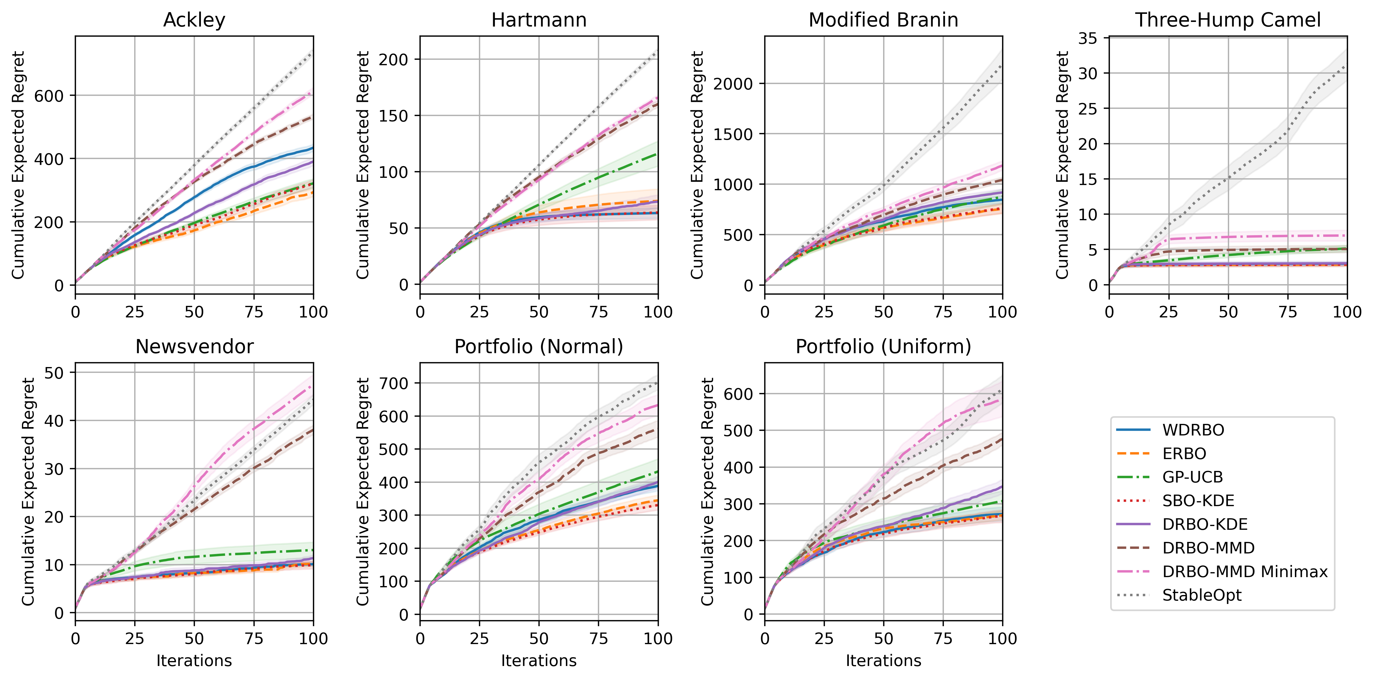
Figure 3: Mean and standard error of the cumulative expected regret.

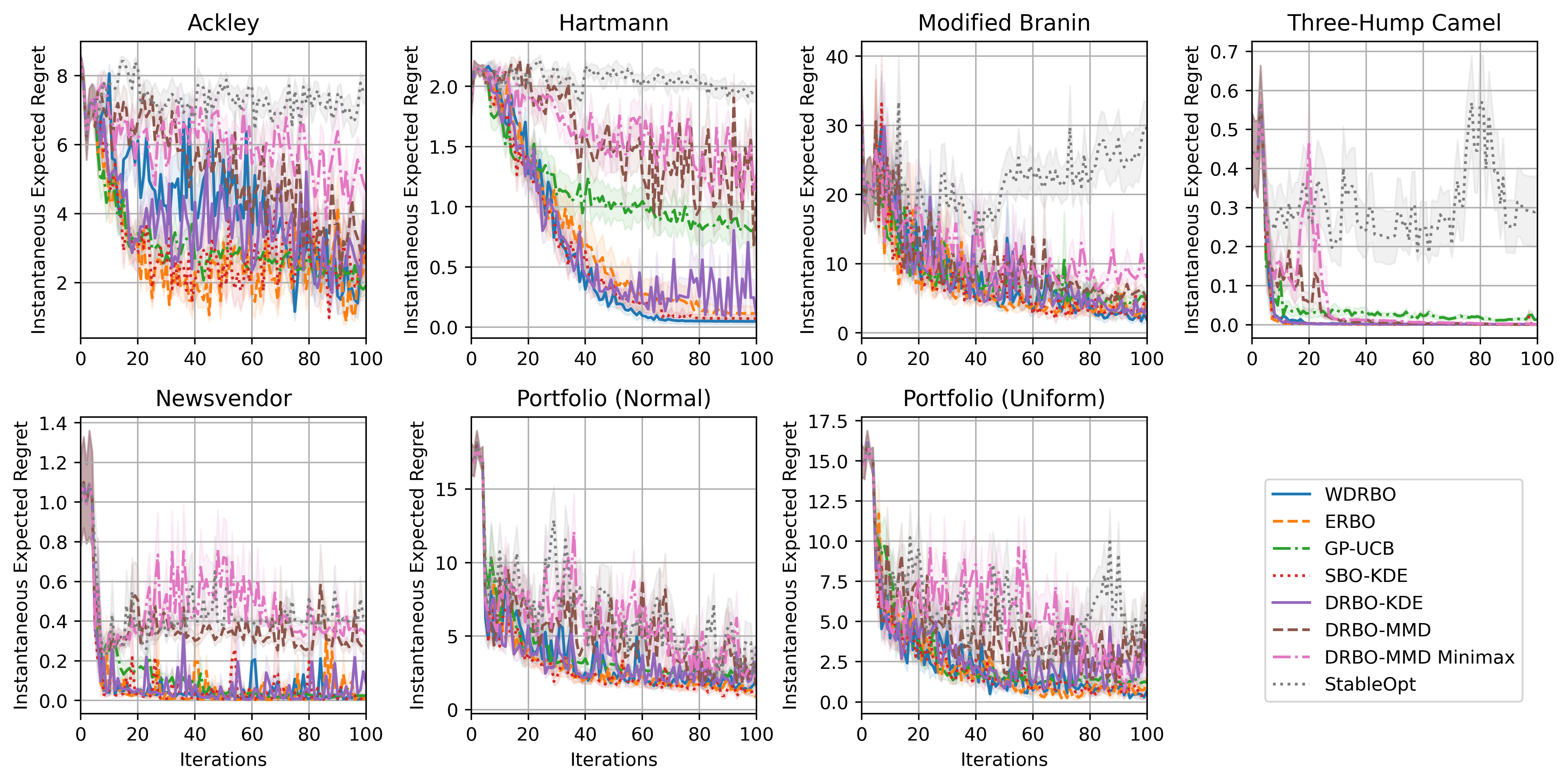
Figure 4: Mean and standard error of the instantaneous expected regret.

References

- Ueno et al. (2016) Tsuyoshi Ueno, Trevor David Rhone, Zhufeng Hou, Teruyasu Mizoguchi, and Koji Tsuda. Combo: An efficient bayesian optimization library for materials science. Materials discovery, 4:18–21, 2016.
- Li et al. (2019) Cheng Li, Santu Rana, Sunil Gupta, Vu Nguyen, Svetha Venkatesh, Alessandra Sutti, David Rubin, Teo Slezak, Murray Height, Mazher Mohammed, et al. Accelerating experimental design by incorporating experimenter hunches. arXiv preprint arXiv:1907.09065, 2019.
- Ru et al. (2020) Binxin Ru, Ahsan Alvi, Vu Nguyen, Michael A Osborne, and Stephen Roberts. Bayesian optimisation over multiple continuous and categorical inputs. In International Conference on Machine Learning, pages 8276–8285. PMLR, 2020.
- Shahriari et al. (2015) Bobak Shahriari, Kevin Swersky, Ziyu Wang, Ryan P Adams, and Nando De Freitas. Taking the human out of the loop: A review of bayesian optimization. Proceedings of the IEEE, 104(1):148–175, 2015.
- Krause and Ong (2011) Andreas Krause and Cheng Ong. Contextual gaussian process bandit optimization. Advances in neural information processing systems, 24, 2011.
- Valko et al. (2013) Michal Valko, Nathaniel Korda, Rémi Munos, Ilias Flaounas, and Nelo Cristianini. Finite-time analysis of kernelised contextual bandits. arXiv preprint arXiv:1309.6869, 2013.
- Kirschner and Krause (2019) Johannes Kirschner and Andreas Krause. Stochastic bandits with context distributions. Advances in Neural Information Processing Systems, 32, 2019.
- Rahimian and Mehrotra (2019) Hamed Rahimian and Sanjay Mehrotra. Distributionally robust optimization: A review. arXiv preprint arXiv:1908.05659, 2019.
- Kuhn et al. (2019) Daniel Kuhn, Peyman Mohajerin Esfahani, Viet Anh Nguyen, and Soroosh Shafieezadeh-Abadeh. Wasserstein distributionally robust optimization: Theory and applications in machine learning. In Operations research & management science in the age of analytics, pages 130–166. Informs, 2019.
- Gao et al. (2024) Rui Gao, Xi Chen, and Anton J Kleywegt. Wasserstein distributionally robust optimization and variation regularization. Operations Research, 72(3):1177–1191, 2024.
- Kirschner et al. (2020) Johannes Kirschner, Ilija Bogunovic, Stefanie Jegelka, and Andreas Krause. Distributionally robust bayesian optimization. In International Conference on Artificial Intelligence and Statistics, pages 2174–2184. PMLR, 2020.
- Nguyen et al. (2020) Thanh Nguyen, Sunil Gupta, Huong Ha, Santu Rana, and Svetha Venkatesh. Distributionally robust bayesian quadrature optimization. In International Conference on Artificial Intelligence and Statistics, pages 1921–1931. PMLR, 2020.
- Husain et al. (2024) Hisham Husain, Vu Nguyen, and Anton van den Hengel. Distributionally robust bayesian optimization with -divergences. Advances in Neural Information Processing Systems, 36, 2024.
- Tay et al. (2022) Sebastian Shenghong Tay, Chuan Sheng Foo, Urano Daisuke, Richalynn Leong, and Bryan Kian Hsiang Low. Efficient distributionally robust bayesian optimization with worst-case sensitivity. In International Conference on Machine Learning, pages 21180–21204. PMLR, 2022.
- Huang et al. (2024) Xiaobin Huang, Lei Song, Ke Xue, and Chao Qian. Stochastic bayesian optimization with unknown continuous context distribution via kernel density estimation. In Proceedings of the AAAI Conference on Artificial Intelligence, volume 38, pages 12635–12643, 2024.
- Srinivas et al. (2009) Niranjan Srinivas, Andreas Krause, Sham M Kakade, and Matthias Seeger. Gaussian process optimization in the bandit setting: No regret and experimental design. arXiv preprint arXiv:0912.3995, 2009.
- Srinivas et al. (2012) Niranjan Srinivas, Andreas Krause, Sham M Kakade, and Matthias W Seeger. Information-theoretic regret bounds for gaussian process optimization in the bandit setting. IEEE transactions on information theory, 58(5):3250–3265, 2012.
- Abbasi-Yadkori (2013) Yasin Abbasi-Yadkori. Online learning for linearly parametrized control problems. 2013.
- Whitehouse et al. (2023) Justin Whitehouse, Zhiwei Steven Wu, and Aaditya Ramdas. Improved self-normalized concentration in hilbert spaces: Sublinear regret for gp-ucb. arXiv preprint arXiv:2307.07539, 2023.
- Gao (2023) Rui Gao. Finite-sample guarantees for wasserstein distributionally robust optimization: Breaking the curse of dimensionality. Operations Research, 71(6):2291–2306, 2023.
- Kirschner and Krause (2018) Johannes Kirschner and Andreas Krause. Information directed sampling and bandits with heteroscedastic noise. In Conference On Learning Theory, pages 358–384. PMLR, 2018.
- Bogunovic and Krause (2021) Ilija Bogunovic and Andreas Krause. Misspecified gaussian process bandit optimization. Advances in neural information processing systems, 34:3004–3015, 2021.
- Schölkopf and Smola (2002) Bernhard Schölkopf and Alexander J Smola. Learning with kernels: support vector machines, regularization, optimization, and beyond. MIT press, 2002.
- Williams and Rasmussen (2006) Christopher KI Williams and Carl Edward Rasmussen. Gaussian processes for machine learning, volume 2. MIT press Cambridge, MA, 2006.
- Chowdhury and Gopalan (2017) Sayak Ray Chowdhury and Aditya Gopalan. On kernelized multi-armed bandits. In International Conference on Machine Learning, pages 844–853. PMLR, 2017.
- Vakili et al. (2021) Sattar Vakili, Kia Khezeli, and Victor Picheny. On information gain and regret bounds in gaussian process bandits. In International Conference on Artificial Intelligence and Statistics, pages 82–90. PMLR, 2021.
- Auer (2002) P Auer. Finite-time analysis of the multiarmed bandit problem, 2002.
- Fournier and Guillin (2015) Nicolas Fournier and Arnaud Guillin. On the rate of convergence in wasserstein distance of the empirical measure. Probability theory and related fields, 162(3):707–738, 2015.
- Fournier (2022) Nicolas Fournier. Convergence of the empirical measure in expected wasserstein distance: non asymptotic explicit bounds in . arXiv preprint arXiv:2209.00923, 2022.
- Yang et al. (2020) Zhuoran Yang, Chi Jin, Zhaoran Wang, Mengdi Wang, and Michael I Jordan. On function approximation in reinforcement learning: Optimism in the face of large state spaces. arXiv preprint arXiv:2011.04622, 2020.
- Bogunovic et al. (2018) Ilija Bogunovic, Jonathan Scarlett, Stefanie Jegelka, and Volkan Cevher. Adversarially robust optimization with gaussian processes. Advances in neural information processing systems, 31, 2018.
- Kanagawa et al. (2018) Motonobu Kanagawa, Philipp Hennig, Dino Sejdinovic, and Bharath K Sriperumbudur. Gaussian processes and kernel methods: A review on connections and equivalences. arXiv preprint arXiv:1807.02582, 2018.
- Van Waarde and Sepulchre (2022) Henk J Van Waarde and Rodolphe Sepulchre. Kernel-based models for system analysis. IEEE Transactions on Automatic Control, 68(9):5317–5332, 2022.
- Vershynin (2018) Roman Vershynin. High-dimensional probability: An introduction with applications in data science, volume 47. Cambridge university press, 2018.
- Vakili and Olkhovskaya (2023) Sattar Vakili and Julia Olkhovskaya. Kernelized reinforcement learning with order optimal regret bounds. Advances in Neural Information Processing Systems, 36:4225–4247, 2023.
- Balandat et al. (2020) Maximilian Balandat, Brian Karrer, Daniel Jiang, Samuel Daulton, Ben Letham, Andrew G Wilson, and Eytan Bakshy. Botorch: A framework for efficient monte-carlo bayesian optimization. Advances in neural information processing systems, 33:21524–21538, 2020.
- Diamond and Boyd (2016) Steven Diamond and Stephen Boyd. Cvxpy: A python-embedded modeling language for convex optimization. Journal of Machine Learning Research, 17(83):1–5, 2016.