missing

Abstract.

In this paper, we consider $n$ agents who invest in a general financial market that is free of arbitrage and complete. The aim of each investor is to maximize her expected utility while ensuring, with a specified probability, that her terminal wealth exceeds a benchmark defined by her competitors’ performance. This setup introduces an interdependence between agents, leading to a search for Nash equilibria. In the case of two agents and CRRA utility, we are able to derive all Nash equilibria in terms of terminal wealth. For $n>2$ agents and logarithmic utility we distinguish two cases. In the first case, the probabilities in the constraint are small and we can characterize all Nash equilibria. In the second case, the probabilities are larger and we look for Nash equilibria in a certain set. We also discuss the impact of the competition using some numerical examples. As a by-product, we solve some portfolio optimization problems with probability constraints.

otsep5

Key words:

Nash equilibrium; competitive investment; Value at risk; CRRA utility

Statements and Declarations: The authors have no relevant financial or non-financial interests to disclose. Data sharing is not applicable to this article as no datasets were generated or analyzed during the current study.

1. Introduction

In standard asset allocation problems, a single agent typically invests in a financial market to optimize an objective, such as expected utility or mean-variance. In reality, however, investors are rarely isolated; they are often influenced by their relative performance compared to others. In this paper, we examine a scenario with $n$ agents investing in a shared financial market, where each agent aims to maximize her expected utility while ensuring, with a specified probability, that her terminal wealth exceeds a benchmark defined by her competitors’ performance. For instance, an agent might require that, with $90\%$ probability, her final wealth surpasses the average wealth of her competitors. This setup introduces a strategic layer to the optimization problem, where agents’ objectives are interdependent, leading to a search for Nash equilibria under probabilistic constraints. Consequently, our framework integrates strategic interactions among agents with value-at-risk constraints.

Before we have a closer look at our results, let us mention the related literature. There have been a number of papers recently which consider strategic interactions between agents in asset allocation problems. The motivation stems from Brown et al., (2001) and Kempf and Ruenzi, (2008). The majority of papers model the interaction by maximizing the expected utility of relative wealth in financial markets of Black Scholes type. Relative wealth may be measured by a linear function of the terminal wealths of all agents, see e.g. Espinosa and Touzi, (2015) and Espinosa, (2010), or by a multiplicative function of the terminal wealths, see e.g. Basak and Makarov, (2014). For example Basak and Makarov, (2015) consider two agents investing in a Black Scholes model and maximizing the power utility of the ratio of both wealths. The difference between own wealth and arithmetic mean of other agents’ wealth has been treated in Espinosa and Touzi, (2015). Lacker and Zariphopoulou, (2019) investigate a model where each agent has her own financial market and consider the corresponding mean-field approach. This work has later been extended to investment-consumption in Lacker and Soret, (2020). Fu and Zhou, (2023) and Fu, (2023) provide a relation between Nash equilibria and systems of forward backward stochastic differential equations for agents with power utility and multiplicative relative performance for investment and consumption. Forward utilities with competition are for example considered in Musiela and Zariphopoulou, (2006), Dos Reis and Platonov, (2021) and Anthropelos et al., (2022). Models with more general financial market have been treated in Bäuerle and Göll, (2023), Kraft et al., (2020), Hu and Zariphopoulou, (2022), Aydoğan and Steffensen, (2024). Papers which model in addition price impacts of the investors are Bäuerle and Göll, (2024) and Curatola, (2024).

On the other hand, there is a stream of literature considering benchmark and value-at-risk constraints for one agent problems. For example Basak and Shapiro, (2001) maximize expected utility under the constraint that, with a certain probability, the terminal wealth is above a given deterministic threshold. This is equivalent to requiring that the value-at-risk at the terminal time of the wealth is below a threshold. Gabih et al., (2005, 2009, 2006) consider a similar point of view replacing the value-at-risk by expected shortfall and Sass and Wunderlich, (2010) and Bäuerle and Chen, (2023) extend this situation to problems with partial information.

In our model, we combine these two aspects. We consider $n$ agents who invest into the same financial market. We do not need a specific model for this market. It should be free of arbitrage and complete. The agents aim at maximizing their expected utility at terminal time $T$. Most of the paper is on logarithmic utility, but we also consider power utility. As a constraint, the probability that one’s wealth exceeds a linear combination of the other agents’ wealth is bounded from below. Thus, we adapt the model of Basak and Shapiro, (2001) to include relative concerns by replacing the constant solvency level in the optimization problem of agent $i$ by a weighted arithmetic mean of the other $n-1$ agents’ terminal wealth. Bell and Cover, (1980) consider a simple static two-person zero sum game where the payoff is the probability of beating the opponent’s outcome. There are also links to what is known as Colonel Blotto games, see Kovenock and Roberson, (2021). We incorporate the constraint

$$\mathbb{P}\Big{(}X_{i}\geq\sum_{j\neq i}\beta_{j}X_{j}\Big{)}\geq\alpha_{i}$$ (1.1)

into the optimization problem of agent $i$, where $\alpha_{i}\in[0,1]$ and $\beta_{j}\in(0,1)$ for all $i,j\in\{1,\ldots,n\}$. By $X_{j}$ we denote the terminal wealth of agent $j\in\{1,\ldots,n\}$. Thus, in a fraction of $\alpha_{i}$ of the possible market scenarios, agent $i$ attains a terminal wealth which is at least as large as the weighted average of her competitors’ terminal wealth. The objective function of agent $i$ is given by the expected utility $\mathbb{E}U(X_{i})$ of her terminal wealth where $U$ is a CRRA utility. The parameters $\beta_{j}$ in (1.1) are custom to each agent $j$, but not to agent $i$, meaning that the weight assigned to agent $j$ is the same in the optimization of agent $i$ for any $i\neq j$. A possible choice is $\beta_{j}=\frac{1}{n-1}$, but we allow for more generality at this point. It is, for example, possible to consider weights in terms of the initial capital invested by the agents so that a larger initial investment goes along with a larger weight assigned to the corresponding agent. In contrast to the parameters $\beta_{j}$, $j=1,\ldots,n$, the level $\alpha_{i}\in[0,1]$ is chosen by agent $i$ herself. If $\alpha_{i}$ is chosen close to $1$, agent $i$ wants to insure her terminal wealth against the other agents’ wealth in almost all possible scenarios, while a value $\alpha_{i}$ close to $0$ implies that she does not care as much about her performance with respect to the others. We look for Nash equilibria for this problem in terms of the final wealth. Depending on the specific parameters there are multiple or unique Nash equilibria. In the case of two agents, we obtain rather explicit results and are able to determine all Nash equilibria. In particular some discontinuity phenomena show up. In case of a logarithmic utility, as soon as some probabilities for the constraints are less than one, the structure of the classical optimal terminal wealth is enforced in the Nash equilibrium. The situation with many agents is considerably more difficult. We have to distinguish how large the probabilities for the constraints are. If the sum of all probabilities is at most one, the wealth constraints for the agents will be satisfied on disjoint events for all Nash equilibria.

This paper is organized as follows. In the next section, we comment on the underlying financial market. Section 3 deals with the competition of two agents. We consider logarithmic and power utility there and derive all Nash equilibria rather explicitly. Section 4 is then dedicated to the $n$ agent case with $n\geq 3.$ In this section, we have to distinguish the cases $\alpha_{1}+\ldots+\alpha_{n}\leq 1$ and $\alpha_{1}+\ldots+\alpha_{n}>1.$ While we are able to determine the structure of all Nash equilibria in the first case, we restrict to searching for Nash equilibria of specific type in the second case. Section 5 deals with the special case of one agent aiming to beat a fixed stochastic benchmark with given probability. The last section discusses some numerical results and the appendix provides some auxiliary results.

2. Financial market

We do not introduce a specific financial market, but assume that it is free of arbitrage and complete and that the underlying probability space is continuous. An important example is the Black Scholes market which consists of a riskless bond with interest rate $r$, where we set $r=0$, and $d$ stocks. Thus, if $W=(W_{1},\ldots,W_{d})$ is a $d$-dimensional Brownian motion, then the price processes for stocks $k=1,\ldots,d$ are given by

$$\mathrm{d}S_{k}(t)= S_{k}(t)\Big{(}\mu_{k}\,\mathrm{d}t+\sum_{\ell=1}^{d}\sigma_{k\ell}\,\mathrm{d}W_{\ell}(t)\Big{)},$$

where $S_{k}(0)=1$, $\sigma_{k\ell}\geq 0$. By $\mu=(\mu_{1},\ldots,\mu_{d})\in\mathbb{R}^{d}$ we denote the drift vector and by $\sigma=(\sigma_{k\ell})_{1\leq k,\ell\leq d}$ the volatility matrix, which has to be regular. But as mentioned before, this is just a special example. We assume that all random variables are defined on a probability space $(\Omega,\mathcal{F},\mathbb{P})$ where $\Omega$ is continuous, e.g. $\Omega=\mathbb{R}$ and $\mathcal{F}=\mathcal{F}_{T}^{W}$ is generated by the Brownian motions up to time $T$. By $Z_{T}$ we denote the state price density of the financial market. The price at time $t=0$ of a contingent claim $H$ which is an integrable, $\mathcal{F}$-measurable random variable, is thus given by $\mathbb{E}[Z_{T}H].$ In the example of a Black Scholes market with zero interest, this would be

$$Z_{T}=\exp\Big{(}-\gamma^{\top}W_{T}-\frac{1}{2}\|\gamma\|^{2}T\Big{)}$$

with $\gamma=\sigma^{-1}\mu\in\mathbb{R}^{d}.$ Trading strategies are defined as $(\mathcal{F}_{t}^{W})-$ progressively measurable processes $(\pi_{t}^{k})$ denoting the amount of money invested at time $t$ in stock $k$. Since we compute the Nash equilibrium in terms of terminal wealths of the agents, we do not have to be specific about the financial market. The $\mathcal{F}$-measurable random variable $X_{i}$ always denotes the terminal wealth of agent $i$ at time $T$. Since the financial market is complete, all $\mathcal{F}$-measurable and integrable random variables can be attained by a certain portfolio strategy. The initial wealth needed for this portfolio is given by its price $\mathbb{E}[Z_{T}X_{i}].$ For more general semimartingale financial markets which fit into our setup see Bäuerle and Göll, (2023).

3. Two agent case

In this section, we consider the problem with two agents and two different utility functions: logarithmic and power utility. It turns out that there is a significant difference in the solution between these utility functions, though it is well-known that the logarithmic utility can be seen as a limiting case of power utilities.

3.1. Logarithmic utility

We first consider the case where we have $n=2$ agents with a logarithmic utility. Both agents try to maximize their expected utility of terminal wealth $X_{i},i=1,2,$ at time $T$, given a fixed initial capital $x_{0}^{i}>0,i=1,2,$ under the constraint that their respective terminal wealth exceeds, with a certain probability, a fraction of the competitors terminal wealth. Since $T$ is fixed throughout, we delete it from the notation (except for $Z_{T}$). Thus, agent $i$ faces for fixed $X_{j},j\neq i$ with $i,j\in\{1,2\}$, the problem

$$(P_{2})\left\{\begin{array}[]{l}\mathbb{E}\ln(X_{i})\to\max\\ \mathbb{P}(X_{i}\geq\beta_{j}X_{j})\geq\alpha_{i},\\ \mathbb{E}[Z_{T}X_{i}]=x_{0}^{i},\\ X_{i}\mbox{ is }\mathcal{F}-\mbox{measurable,}\end{array}\right.$$

with $\alpha_{i},\beta_{i}\in[0,1]$ for $i=1,2$. The last equation ensures that the wealth $X_{i}$ has price $x_{0}^{i}$, i.e. can be attained by a self-financing strategy with initial wealth $x_{0}^{i}.$ Now we are seeking for a Nash equilibrium in this situation in terms of terminal wealths. Formally, a Nash equilibrium is here defined as follows.

Definition 3.1.

Let $J_{i}(X_{1},X_{2})=\mathbb{E}\ln(X_{i})$ be the objective function of agent $i$, given that $(X_{1},X_{2})$ satisfy the constraints in $(P_{2})$. A feasible pair $(X_{1}^{*},X_{2}^{*})$ of terminal wealths is called a Nash equilibrium, if

$$J_{1}(X_{1}^{*},X_{2}^{*})\geq J_{1}(X_{1},X_{2}^{*}),\quad J_{2}(X_{1}^{*},X_{2}^{*})\geq J_{2}(X_{1}^{*},X_{2})$$ (3.1)

for all admissible pairs $(X_{1},X_{2})$ in $(P_{2})$.

Remark 3.2.

• Without the probability constraint, the optimal terminal wealth in $(P_{2})$ for agent $i=1,2$ is given by

  $$X_{1}^{*}=\frac{x_{0}^{1}}{Z_{T}},\mbox{ and }X_{2}^{*}=\frac{x_{0}^{2}}{Z_{T}}.$$

  This result can be found e.g. in Korn and Korn, (2013).

• Once we have the optimal wealths, they can be replicated by suitable investment strategies due to the completeness of the financial market.

In what follows, we explicitly determine all Nash equilibria. In order to do this, we have to distinguish several parameter cases. Throughout we assume w.l.o.g. that $x_{0}^{1}\geq x_{0}^{2},$ i.e. agent 1 is at least as rich as agent 2.

Case I: $\alpha_{1}=\alpha_{2}=\beta_{1}=\beta_{2}=1$:

In this case with probability one we must have $X_{1}^{*}\geq X_{2}^{*}$ and $X_{2}^{*}\geq X_{1}^{*},$ hence $X_{1}^{*}=X_{2}^{*}$. Obviously, this can only be satisfied when $x_{0}^{1}=x_{0}^{2}.$ However, it is easy to see that any pair $(X,X)$ of $\mathcal{F}$-measurable random variables with price $\mathbb{E}[Z_{T}X]=x_{0}^{1}$ constitutes a Nash equilibrium. This is because for given $X$, the probability constraint already determines the terminal wealth of the second agent. There is nothing to optimize here and the shape of the terminal wealth can be arbitrary.

Case II: $\alpha_{2}=1,\alpha_{1}=1,\beta_{1}\beta_{2}<1$:

Using the result in Appendix 8.1, we obtain that the mutual best responses have to be of the form:

$$X_{1}^{*}=\max\Big{\{}\beta_{2}X_{2}^{*},\frac{\lambda_{1}}{Z_{T}}\Big{\}},\quad X_{2}^{*}=\max\Big{\{}\beta_{1}X_{1}^{*},\frac{\lambda_{2}}{Z_{T}}\Big{\}}$$ (3.2)

for some $\lambda_{1},\lambda_{2}>0.$ Since $\beta_{1}\beta_{2}<1$, this implies

$$X_{1}^{*}=\frac{1}{Z_{T}}\max\{\beta_{2}\lambda_{2},\lambda_{1}\},\quad X_{2}^{*}=\frac{1}{Z_{T}}\max\{\beta_{1}\lambda_{1},\lambda_{2}\}.$$ (3.3)

Distinguishing the different cases where the maxima are attained and respecting the self-financing conditions $\mathbb{E}[X_{1}^{*}Z_{T}]=x_{0}^{1},\mathbb{E}[X_{2}^{*}Z_{T}]=x_{0}^{2},$ we can see that we obtain a solution only in the case of $x_{0}^{2}\geq\beta_{1}x_{0}^{1}$ and the unique Nash equilibrium (here and elsewhere uniqueness is always up to sets of probability zero) is given by

$$X_{1}^{*}=\frac{x_{0}^{1}}{Z_{T}}\mbox{ and }X_{2}^{*}=\frac{x_{0}^{2}}{Z_{T}}.$$ (3.4)

Case III: $\alpha_{2}=1,\alpha_{1}<1,\beta_{1}\beta_{2}\leq 1$:

Using the result in Appendix 8.1, we obtain that the mutual best responses have to be of the form:

$$X_{1}^{*} =\max\Big{\{}\mathbbm{1}_{A_{1}}\beta_{2}X_{2}^{*},\frac{\lambda_{1}}{Z_{T}}\Big{\}},$$ (3.5)

$$X_{2}^{*} =\max\Big{\{}\beta_{1}X_{1}^{*},\frac{\lambda_{2}}{Z_{T}}\Big{\}},$$ (3.6)

where $\mathbb{P}(A_{1})=\alpha_{1}$ and $\lambda_{1},\lambda_{2}>0.$ We can plug in (3.6) into (3.5) to obtain the following expression:

$$X_{1}^{*} =\max\Big{\{}\mathbbm{1}_{A_{1}}\beta_{2}\max\Big{\{}\beta_{1}X_{1}^{*},\frac{\lambda_{2}}{Z_{T}}\Big{\}},\frac{\lambda_{1}}{Z_{T}}\Big{\}}.$$

Let us first assume that $\beta_{1}\beta_{2}<1$. In this case we obtain:

$$X_{1}^{*}=\frac{1}{Z_{T}}\Big{(}\mathbbm{1}_{A_{1}}\max\{\beta_{2}\lambda_{2},\lambda_{1}\}+\mathbbm{1}_{A_{1}^{c}}\lambda_{1}\Big{)}$$

and in return

$$X_{2}^{*} =\frac{1}{Z_{T}}\max\{\beta_{1}\lambda_{1},\lambda_{2}\}.$$

Distinguishing the different cases where the maxima are attained and respecting the self-financing conditions $\mathbb{E}[X_{1}^{*}Z_{T}]=x_{0}^{1},\mathbb{E}[X_{2}^{*}Z_{T}]=x_{0}^{2},$ we can see that we obtain a solution only in the case of $x_{0}^{2}\geq\beta_{1}x_{0}^{1}$ and the unique Nash equilibrium is given by

$$X_{1}^{*}=\frac{x_{0}^{1}}{Z_{T}}\mbox{ and }X_{2}^{*}=\frac{x_{0}^{2}}{Z_{T}}.$$ (3.7)

Thus, we obtain a Nash equilibrium only when the wealth of the second agent is not too small. In the case $\beta_{1}\beta_{2}=1$ we must have $\mathbb{P}(X_{2}\geq X_{1})=1$ which implies, since $x_{0}^{1}\geq x_{0}^{2}$, that $X_{1}^{*}=X_{2}^{*}$ and necessarily $x_{0}^{1}=x_{0}^{2}.$ Thus, the best response to $X$ in $(P_{2})$ has to be $X$ again. Now consider Lemma 8.2. Let $M_{\lambda}^{X}:=\{X\leq\lambda/Z_{T}\}$ and suppose that $X^{*}$ is the best response to $X$. Obviously $X=X^{*}$ a.s. implies $M_{\lambda}^{X}=M_{\lambda}^{X^{*}}.$ However, if $\mathbb{P}(X\neq x_{0}^{1}/Z_{T})>0$ then $(M_{\lambda_{\alpha}}^{X^{*}})^{c}\cap M_{\lambda_{\alpha}}^{X}\neq\emptyset$ which is a contradiction. Hence $X^{*}=x_{0}^{1}/Z_{T}$ and the Nash equilibrium is again as in (3.7).

Case IV: $\alpha_{1}\leq 1,\alpha_{2}<1,\beta_{1}\beta_{2}\leq 1$:

This case requires more work. First we note that due to the result in Appendix 8.1, we obtain that the mutual best responses have to be of the form:

$$X_{1}^{*} =\max\Big{\{}\mathbbm{1}_{A_{1}}\beta_{2}X_{2}^{*},\frac{\lambda_{1}}{Z_{T}}\Big{\}}=\mathbbm{1}_{A_{1}}\max\Big{\{}\beta_{2}X_{2}^{*},\frac{\lambda_{1}}{Z_{T}}\Big{\}}+\mathbbm{1}_{A_{1}^{c}}\frac{\lambda_{1}}{Z_{T}},$$ (3.8)

$$X_{2}^{*} =\max\Big{\{}\mathbbm{1}_{A_{2}}\beta_{1}X_{1}^{*},\frac{\lambda_{2}}{Z_{T}}\Big{\}}=\mathbbm{1}_{A_{2}}\max\Big{\{}\beta_{1}X_{1}^{*},\frac{\lambda_{2}}{Z_{T}}\Big{\}}+\mathbbm{1}_{A_{2}^{c}}\frac{\lambda_{2}}{Z_{T}},$$ (3.9)

where $\mathbb{P}(A_{i})=\alpha_{i},i=1,2$ and $\lambda_{1},\lambda_{2}>0.$ Plugging (3.8) into (3.9) yields:

$$X_{2}^{*}=\max\Big{\{}\mathbbm{1}_{A_{1}\cap A_{2}}\max\Big{\{}\beta_{1}\beta_{2}X_{2}^{*},\frac{\beta_{1}\lambda_{1}}{Z_{T}}\Big{\}}+\mathbbm{1}_{A_{1}^{c}\cap A_{2}}\frac{\lambda_{1}\beta_{1}}{Z_{T}},\mathbbm{1}_{A_{2}}\frac{\lambda_{2}}{Z_{T}}\Big{\}}+\mathbbm{1}_{A_{2}^{c}}\frac{\lambda_{2}}{Z_{T}}.$$ (3.10)

We now assume that $\beta_{1}\beta_{2}<1.$ Simplifying this expression, we end up with

$$X_{2}^{*}=\frac{1}{Z_{T}}\Big{(}\lambda_{2}\mathbbm{1}_{A_{2}^{c}}+\max\{\beta_{1}\lambda_{1},\lambda_{2}\}\mathbbm{1}_{A_{2}}\Big{)}.$$ (3.11)

This in turn implies

$$X_{1}^{*}=\frac{1}{Z_{T}}\Big{(}\lambda_{1}\mathbbm{1}_{A_{1}^{c}}+\max\{\beta_{2}\lambda_{2},\lambda_{1}\}\mathbbm{1}_{A_{1}}\Big{)}.$$ (3.12)

We also have to respect the self-financing condition which implies the equations

$$\mathbb{E}[X_{1}^{*}Z_{T}] =\lambda_{1}(1-\alpha_{1})+\max\{\beta_{2}\lambda_{2},\lambda_{1}\}\alpha_{1}=x_{0}^{1},$$ (3.13)

$$\mathbb{E}[X_{2}^{*}Z_{T}] =\lambda_{2}(1-\alpha_{2})+\max\{\beta_{1}\lambda_{1},\lambda_{2}\}\alpha_{2}=x_{0}^{2}.$$ (3.14)

Depending on where the maxima are attained, we obtain essentially two cases.

First consider $\lambda_{1}\geq\lambda_{2}\geq\beta_{1}\lambda_{1}.$ Here it follows that

$$X_{1}^{*}=\frac{x_{0}^{1}}{Z_{T}}\mbox{ and }X_{2}^{*}=\frac{x_{0}^{2}}{Z_{T}},$$ (3.15)

and that $x_{0}^{2}\geq\beta_{1}x_{0}^{1}$ (note that $x_{0}^{1}\geq x_{0}^{2}$ throughout). The other case which yields a solution is $\beta_{1}\lambda_{1}\geq\lambda_{2}.$ In this case

$$X_{1}^{*}=\frac{x_{0}^{1}}{Z_{T}}\mbox{ and }X_{2}^{*}=\beta_{1}\frac{x_{0}^{1}}{Z_{T}}\mathbbm{1}_{A_{2}}+\frac{\lambda_{2}}{Z_{T}}\mathbbm{1}_{A_{2}^{c}}$$ (3.16)

with $\lambda_{2}=(x_{0}^{2}-\beta_{1}x_{0}^{1}\alpha_{2})/(1-\alpha_{2})\in[0,x_{0}^{2}].$ This case occurs when we have $x_{0}^{1}\beta_{1}\geq x_{0}^{2}\geq x_{0}^{1}\beta_{1}\alpha_{2}.$ Note that the position of the set $A_{2}$ is arbitrary i.e. we obtain an infinite number of Nash equilibria in this case.

The case $\beta_{1}\beta_{2}=1$ remains. Proceeding as before, we conclude that only the case $\lambda_{1}\geq\lambda_{2}$ leads to solutions which are of the form

$$X_{1}^{*} =\frac{\lambda_{1}}{Z_{T}}\mathbbm{1}_{(A_{1}\cap A_{2})^{c}}+\max\Big{\{}X_{2}^{*},\frac{\lambda_{1}}{Z_{T}}\Big{\}}\mathbbm{1}_{A_{1}\cap A_{2}},$$ (3.17)

$$X_{2}^{*} =\frac{\lambda_{1}}{Z_{T}}\mathbbm{1}_{A_{2}\setminus A_{1}}+\max\Big{\{}X_{2}^{*},\frac{\lambda_{1}}{Z_{T}}\Big{\}}\mathbbm{1}_{A_{1}\cap A_{2}}+\frac{\lambda_{2}}{Z_{T}}\mathbbm{1}_{A_{2}^{c}}.$$ (3.18)

By contradiction we obtain that the maximum in the preceding expression has to be $\lambda_{1}/Z_{T}.$ As a result $X_{1}^{*}=x_{0}^{1}/Z_{T}$ and the solution has the same form as before.

We summarize our findings in the following theorem:

Theorem 3.3 (Logarithmic utility).

Let $\alpha_{i},\,\beta_{i}\in[0,1],\,x_{0}^{i}>0,\,i=1,2.$ If $x_{0}^{2}<\alpha_{2}\beta_{1}x_{0}^{1}$, there is no Nash equilibrium. Otherwise, i.e. if $x_{0}^{2}\geq\alpha_{2}\beta_{1}x_{0}^{1}$, there exist three cases.

• If $\alpha_{i}=1,\,\beta_{i}=1,\,i=1,2,$ there are infinitely many Nash equilibria of the form $(X,X)$, where $X$ is an $\mathcal{F}$-measurable random variable with $\mathbb{E}[Z_{T}X]=x_{0}^{1}$.

• If either $\alpha_{i}=1,\,i=1,2,\,\beta_{1}\beta_{2}<1$ or $\alpha_{1}<1,\,\alpha_{2}=1,$ the unique Nash equilibrium is given by

  $$X_{1}^{*}=\frac{x_{0}^{1}}{Z_{T}}\mbox{ and }X_{2}^{*}=\frac{x_{0}^{2}}{Z_{T}}.$$

• If $\alpha_{1}\leq 1,\,\alpha_{2}<1,$ there are two additional cases. If $x_{0}^{2}\geq\beta_{1}x_{0}^{1}$, the unique Nash equilibrium is given by

  $$X_{1}^{*}=\frac{x_{0}^{1}}{Z_{T}}\mbox{ and }X_{2}^{*}=\frac{x_{0}^{2}}{Z_{T}}.$$

  Otherwise, i.e. if $x_{0}^{2}<\beta_{1}x_{0}^{1}$ there are infinitely many Nash equilibria of the form

  $$X_{1}^{*}=\frac{x_{0}^{1}}{Z_{T}}\mbox{ and }X_{2}^{*}=\frac{\beta_{1}x_{0}^{1}}{Z_{T}}\mathbbm{1}_{A_{2}}+\frac{x_{0}^{2}-\alpha_{2}\beta_{1}x_{0}^{1}}{(1-\alpha_{2})Z_{T}}\mathbbm{1}_{A_{2}^{c}}$$

  with $A_{2}\in\mathcal{F}$ such that $\mathbb{P}(A_{2})=\alpha_{2}.$

Remark 3.4.

• Note that in case a) of the previous theorem, the condition $x_{0}^{2}\geq\alpha_{2}\beta_{1}x_{0}^{1}$ already implies that $x_{0}^{1}=x_{0}^{2}$. Moreover, it also states that, as long as $x_{0}^{2}\geq\beta_{1}x_{0}^{1}$, the optimal solution $X_{i}^{*}=x_{0}^{i}Z_{T}^{-1}$, $i=1,2,$ to the unconstrained problem is always a Nash equilibrium. If at least one of the parameters $\alpha_{i},\beta_{i},\,i=1,2,$ is strictly smaller than $1$, it is the unique Nash equilibrium.

• There is a very fundamental difference between Case I and Case II when $\beta_{1}\beta_{1}=1$ but $\alpha_{1}<1$ instead of $\alpha_{1}=1$. As soon as as there is no strict dominance of the final wealths required, the form $\lambda/Z_{T}$ of the optimal wealth in the single agent portfolio optimization problem carries through to the Nash equilibrium.

• Note that in case of a logarithmic utility there can be an infinite number of different Nash equilibria. In particular in Case III, it does not matter where the set $A_{2}$ exactly is. This is different for other utility functions, see the next section with power utility.

• It is possible to pick other criteria to choose one of the Nash equilibria in case there are several ones. For example in Case I it makes sense to choose the same Nash equilibrium as in b), since it maximizes the expected utility. In Case IV the expected utility of all Nash equilibria are the same. Hence one could simply look for the Nash equilibrium which maximizes $\mathbb{E}[X_{2}^{*}].$ It is easy to see (note that here $\beta_{1}x_{0}^{1}>x_{0}^{2}$) that this is achieved by choosing $A_{2}:=\{Z_{T}\leq z_{\alpha_{2}}\}$ where $z_{\alpha_{2}}$ is the $\alpha_{2}-$quantile of $Z_{T}$, i.e. $\mathbb{P}(Z_{T}\leq z_{\alpha_{2}})={\alpha_{2}}$.

3.2. Power utility

We consider now the same problem with power utility for the agents. Note that we use the same parameter for the utility function for both agents. More precisely, we consider for $U(x)=\frac{1}{1-\gamma}x^{1-\gamma},\,\gamma\in(0,1),$ the individual portfolio problems

$$(P_{2})\left\{\begin{array}[]{l}\mathbb{E}U(X_{i})\to\max\\ \mathbb{P}(X_{i}\geq\sum_{j\neq i}\beta_{j}X_{j})\geq\alpha_{i},\\ \mathbb{E}[Z_{T}X_{i}]=x_{0}^{i},\\ X_{i}\mbox{ is }\mathcal{F}-\mbox{measurable,}\end{array}\right.$$

for $i=1,2$. For notational convenience, we abbreviate $\varepsilon_{\gamma}:=\mathbb{E}\big{[}Z_{T}^{1-1/\gamma}\big{]}.$

As in the previous case of logarithmic utility, it is easy to see that for $x_{0}^{1}\geq\beta_{2}x_{0}^{2}\geq\beta_{1}\beta_{2}x_{0}^{1}$ the optimal terminal wealths without constraint constitute a Nash equilibrium, i.e.

$$X_{1}^{*}=\frac{x_{0}^{1}}{\varepsilon_{\gamma}}Z_{T}^{-1/\gamma},\mbox{ and }X_{2}^{*}=\frac{x_{0}^{2}}{\varepsilon_{\gamma}}Z_{T}^{-1/\gamma},$$

since $I(x):=x^{-1/\gamma}$ is the inverse function of $U^{\prime}$ (see e.g. Korn and Korn,, 2013).

We concentrate now on the interesting case which is determined by the parameters $\beta_{1}\beta_{2}<1$ and

$$\beta_{1}x_{0}^{1}>x_{0}^{2}\geq\frac{\beta_{1}x_{0}^{1}}{\varepsilon_{\gamma}}\int_{Z_{T}\geq z_{1-\alpha_{2}}}Z_{T}^{1-1/\gamma}d\mathbb{P},$$ (3.19)

where $z_{1-\alpha_{2}}$ is the $(1-\alpha_{2})-$quantile of $Z_{T}$, i.e. $\mathbb{P}(Z_{T}\leq z_{1-\alpha_{2}})=1-{\alpha_{2}}$. Since $Z_{T}>0$ we necessarily have that $z_{1-\alpha_{2}}>0.$

Theorem 3.5 (Power utility).

If $\beta_{1}\beta_{2}<1$ and the inequality in (3.19) holds true, the unique Nash equilibrium is given by

$$X_{1}^{*}=\frac{x_{0}^{1}}{\varepsilon_{\gamma}}Z_{T}^{-1/\gamma},\mbox{ and }X_{2}^{*}=\left\{\begin{array}[]{cr}(\lambda_{2}Z_{T})^{-1/\gamma},&Z_{T}<z_{1-\alpha_{2}},\\ \beta_{1}\frac{x_{0}^{1}}{\varepsilon_{\gamma}}Z_{T}^{-1/\gamma},&Z_{T}\geq z_{1-\alpha_{2}},\end{array}\right.$$ (3.20)

where $\lambda_{2}>0$ is such that $\mathbb{E}[Z_{T}X_{2}^{*}]=x_{0}^{2}$.

Proof.

Using Lemma 8.1 and rearranging the terms, we obtain that a Nash equilibrium is necessarily of the form

$$X_{1}^{*} ={Z_{T}}^{-1/\gamma}\Big{(}\lambda_{1}\mathbbm{1}_{A_{1}^{c}}+\max\{\beta_{2}\lambda_{2},\lambda_{1}\}\mathbbm{1}_{A_{1}}\Big{)},$$

$$X_{2}^{*} ={Z_{T}}^{-1/\gamma}\Big{(}\lambda_{2}\mathbbm{1}_{A_{2}^{c}}+\max\{\beta_{1}\lambda_{1},\lambda_{2}\}\mathbbm{1}_{A_{2}}\Big{)}$$

for some $\lambda_{1},\lambda_{2}>0$ and measurable sets $A_{1},A_{2}$ with probability $\mathbb{P}(A_{i})=\alpha_{1},i=1,2.$ Distinguishing the cases where the maximum is attained, it is possible to see that only the case $\lambda_{1}\geq\beta_{2}\lambda_{2}$ yields a solution. Moreover, it follows that

$$X_{1}^{*}=\frac{x_{0}^{1}}{\varepsilon_{\gamma}}Z_{T}^{-1/\gamma}.$$

In order to determine the precise form of $X_{2}^{*}$, we will proceed in a different way as in the logarithmic case. This is necessary, because in the power setting it will turn out that it really matters where the region is located precisely where the probability constraint is satisfied. This does not follow from Lemma 8.1.
We write $\lambda_{1}:=U^{\prime}(x_{0}^{1}/\varepsilon_{\gamma})$, i.e. $I(\lambda_{1})=x_{0}^{1}/\varepsilon_{\gamma}.$ It follows that $I(\lambda_{2})<\beta_{1}I(\lambda_{1})$, because otherwise the price of $X_{2}^{*}$ would be larger or equal than $\beta_{1}x_{0}^{1}$ which contradicts our assumption. This implies $\lambda_{2}>\lambda_{1}\beta_{1}^{-\gamma}$. It remains to prove that $X_{2}^{*}$ is the best response to $X_{1}^{*}$. Thus, we consider the following function

$$L(X,\lambda_{2},\eta_{2}):=U(X)-\lambda_{2}Z_{T}X+\eta_{2}\mathbbm{1}\{X\geq\beta_{1}I(\lambda_{1}Z_{T})\},$$

where

$$\eta_{2}:=U(I(\lambda_{2}z_{1-\alpha_{2}}))-U(\beta_{1}I(\lambda_{1}z_{1-\alpha_{2}}))+\lambda_{2}z_{1-\alpha_{2}}\Big{(}\beta_{1}I(\lambda_{1}z_{1-\alpha_{2}})-I(\lambda_{2}z_{1-\alpha_{2}})\Big{)}$$

and $\lambda_{1},\lambda_{2}$ as before. Note that $\eta_{2}\geq 0$ since

$$\eta_{2}\geq 0 \Leftrightarrow U(I(\lambda_{2}z_{1-\alpha_{2}}))-U(\beta_{1}I(\lambda_{1}z_{1-\alpha_{2}}))\geq\lambda_{2}z_{1-\alpha_{2}}\Big{(}I(\lambda_{2}z_{1-\alpha_{2}})-\beta_{1}I(\lambda_{1}z_{1-\alpha_{2}})\Big{)}$$

$$\Leftrightarrow\frac{U(I(\lambda_{2}z_{1-\alpha_{2}}))-U(\beta_{1}I(\lambda_{1}z_{1-\alpha_{2}}))}{I(\lambda_{2}z_{1-\alpha_{2}})-\beta_{1}I(\lambda_{1}z_{1-\alpha_{2}})}\leq\lambda_{2}z_{1-\alpha_{2}}$$

$$\Leftrightarrow U^{\prime}(\xi)\leq\lambda_{2}z_{1-\alpha_{2}}$$

for some $\xi\in(I(\lambda_{2}z_{1-\alpha_{2}}),\beta_{1}I(\lambda_{1}z_{1-\alpha_{2}})).$ Because $U^{\prime}$ is non-increasing, we obtain $U^{\prime}(\xi)\leq U^{\prime}(I(\lambda_{2}z_{1-\alpha_{2}}))=\lambda_{2}z_{1-\alpha_{2}}.$ Now we can show that for any other admissible terminal wealth $X_{2}$ we obtain

$$\mathbb{E}U(X_{2}^{*})-\mathbb{E}U(X_{2})\geq\mathbb{E}L(X_{2}^{*},\lambda_{2},\eta_{2})-\mathbb{E}L(X_{2},\lambda_{2},\eta_{2})\geq 0,$$

since $X_{2}^{*}$ maximizes $X\mapsto L(X,\lambda_{2},\eta_{2})$ pointwise (see App. 8.3) which implies that $X_{2}^{*}$ maximizes the objective of agent 2 under the VaR-based constraint. Now it only remains to discuss the existence of $\lambda_{2}>0$ such that $\mathbb{E}[Z_{T}X_{2}^{*}]=x_{0}^{2}$. We can solve

$$\mathbb{E}[Z_{T}X_{2}^{*}]=\lambda_{2}^{-1/\gamma}\mathbb{E}\Big{[}Z_{T}^{1-1/\gamma}\mathbbm{1}\{Z_{T}<z_{1-\alpha_{2}}\}\Big{]}+\frac{\beta_{1}x_{0}^{1}}{\varepsilon_{\gamma}}\mathbb{E}\Big{[}Z_{T}^{1-1/\gamma}\mathbbm{1}\{Z_{T}\geq z_{1-\alpha_{2}}\}\Big{]}=x_{0}^{2}$$

for $\lambda_{2}$ to obtain

$$\lambda_{2}=\mathbb{E}\Big{[}Z_{T}^{1-1/\gamma}\mathbbm{1}\{Z_{T}<z_{1-\alpha_{2}}\}\Big{]}^{\gamma}\bigg{(}x_{0}^{2}-\frac{\beta_{1}x_{0}^{1}}{\varepsilon_{\gamma}}\mathbb{E}\Big{[}Z_{T}^{1-1/\gamma}\mathbbm{1}\{Z_{T}\geq z_{1-\alpha_{2}}\}\Big{]}\bigg{)}^{-\gamma}.$$

Since (3.19) holds, we have $\lambda_{2}>0$ which concludes the proof. ∎

Remark 3.6.

Note that for power utility, in contrast to logarithmic utility, the position of the set $A$ that guarantees that the probability constraint is satisfied is not arbitrary. This is remarkable since the limit $\gamma\to 1$ results in a logarithmic utility function. Moreover, we can compare the set $\{Z_{T}>z_{1-\alpha_{2}}\}$ on which the constraint is satisfied in the power utility case to the set $\{Z_{T}\leq z_{\alpha_{2}}\}$ discussed in Remark 3.4. There we searched for the set $A_{2}$ with $\mathbb{P}(A_{2})=\alpha_{2}$ that maximizes the expected terminal wealth of agent 2 in the Nash equilibrium under logarithmic utility. On the contrary, the set $\{Z_{T}>z_{1-\alpha_{2}}\}$ found in Theorem 3.5 minimizes the expected terminal wealth discussed in Remark 3.4. Nevertheless, it does not come as a surprise that the constraint is satisfied on the set $\{Z_{T}>z_{1-\alpha_{2}}\}$ since it is ’cheaper’ to satisfy the constraint there as the terminal wealth of agent 1 is decreasing in $Z_{T}$.

4. Multi agent case

Here we consider problem $(P_{2})$ in the case of $n\geq 3$ agents, i.e. for $i=1,\ldots,n$ we look at

$$(P_{n})\left\{\begin{array}[]{l}\mathbb{E}\ln(X_{i})\to\max\\ \mathbb{P}(X_{i}\geq\sum_{j\neq i}\beta_{j}X_{j})\geq\alpha_{i},\\ \mathbb{E}[Z_{T}X_{i}]=x_{0}^{i},\\ X_{i}\mbox{ is }\mathcal{F}-\mbox{measurable,}\end{array}\right.$$

with $\alpha_{i},\beta_{i}\in[0,1]$. Further, we assume w.l.o.g. that the initial capitals of the agents are ordered by $x_{0}^{1}\geq\ldots\geq x_{0}^{n}.$ In particular, we restrict the discussion to the logarithmic utility. Moreover, we assume that for all $i$ we have $\sum_{j\neq i}\beta_{j}\leq 1.$ We are again looking for a Nash equilibrium of investment strategies. The definition for $n$ agents is as follows:

Definition 4.1.

Let $J_{i}(X_{1},\ldots,X_{n})=\mathbb{E}\ln(X_{i})$ be the objective function of agent $i$ given $(X_{1},\ldots,X_{n})$ satisfy the constraints in $(P_{n})$. A feasible vector $(X_{1}^{*},\ldots,X_{n}^{*})$ of terminal wealths is called a Nash equilibrium, if, for all admissible random vectors $(X_{1}^{*},\ldots,X_{i-1}^{*},X_{i},X_{i+1}^{*},\ldots,X_{n}^{*})$ on the right-hand side:

$$J_{i}(X_{1}^{*},\ldots,X_{n}^{*})\geq J_{i}(X_{1}^{*},\ldots,X_{i-1}^{*},X_{i},X_{i+1}^{*},\ldots,X_{n}^{*})$$ (4.1)

for all agents $i.$

We distinguish now the following cases:

4.1. Assume that $\alpha_{1}+\ldots+\alpha_{n}\leq 1$

In this case, the probability constraints of the agents can (and will) be satisfied on disjoint sets.

Theorem 4.2.

If a Nash equilibrium exists, it is of the form

$$X_{i}^{*}=\frac{1}{Z_{T}}\Big{(}\mathbbm{1}_{A_{i}}\max\{x_{0}^{i},\lambda_{\beta}^{-i}\}+\mathbbm{1}_{A_{i}^{c}}\lambda_{i}\Big{)}$$ (4.2)

with $\lambda_{\beta}^{-i}:=\sum_{j\neq i}\beta_{j}\lambda_{j}$, $\mathbb{P}(A_{i})=\alpha_{i}$ and $A_{i}\cap A_{j}=\emptyset$ for $i\neq j.$ Moreover, we have that

$$\lambda_{i}=\frac{1}{1-\alpha_{i}}\Big{(}x_{0}^{i}-\alpha_{i}\max\{x_{0}^{i},\lambda_{\beta}^{-i}\}\Big{)}$$ (4.3)

and $0<\lambda_{i}\leq x_{0}^{i}$, $\alpha_{i}\lambda_{\beta}^{-i}\leq x_{0}^{i}.$

Proof.

In order to determine a Nash equilibrium, we have to solve the best response problem $(P_{n})$ for an arbitrary agent $i$. Suppose that $X_{j},j\neq i,$ are arbitrary given wealths of agents $j$. We can reformulate problem $(P_{n})$ as follows:

$$(P_{n})\left\{\begin{array}[]{l}\mathbb{E}\ln(X_{i})\to\max\\ X_{i}\geq\mathbbm{1}_{A_{i}}\sum_{j\neq i}\beta_{j}X_{j},\\ \mathbb{E}[Z_{T}X_{i}]=x_{0}^{i},\\ X_{i}\mbox{ is }\mathcal{F}-\mbox{measurable,}\\ A_{i}\in\mathcal{F},\mathbb{P}(A_{i})=\alpha_{i}.\end{array}\right.$$

Note that the optimization is over $X_{i}$ and the set $A_{i}$ here. According to Lemma 8.1, an optimal solution is of the form

$$X_{i} =\max\left\{\mathbbm{1}_{A_{i}}X_{\beta}^{-i},\frac{\lambda_{i}}{Z_{T}}\right\}=\mathbbm{1}_{A_{i}}\max\left\{X_{\beta}^{-i},\frac{\lambda_{i}}{Z_{T}}\right\}+\mathbbm{1}_{A_{i}^{c}}\frac{\lambda_{i}}{Z_{T}},$$

where $X_{\beta}^{-i}:=\sum_{j\neq i}\beta_{j}X_{j}$. The maximum construction and the self-financing constraint yield $X_{i}\geq\lambda_{i}/Z_{T}$ and $\lambda_{i}\leq x_{0}^{i}.$ Thus, we obtain that the minimal value of $Z_{T}X_{\beta}^{-i}$ is attained on the set $(\cup_{j\neq i}A_{j})^{c}.$ Taking Lemma 8.2 into account, in order to maximize $\mathbb{E}\ln(X_{i})$ we have to choose $A_{i}$ such that $A_{i}\cap A_{j}=\emptyset$ for $i\neq j.$ Due to the assumption $\alpha_{1}+\ldots+\alpha_{n}\leq 1$, this is possible and the sets $A_{i}$ are disjoint in a Nash equilibrium. In particular we obtain

$$X_{1} = \mathbbm{1}_{A_{1}}\max\left\{X_{\beta}^{-1},\frac{\lambda_{1}}{Z_{T}}\right\}+\mathbbm{1}_{A_{1}^{c}}\frac{\lambda_{1}}{Z_{T}},$$

$$X_{2} = \mathbbm{1}_{A_{2}}\max\bigg{\{}\beta_{1}X_{1}+\sum_{j\geq 3}\beta_{j}X_{j},\frac{\lambda_{2}}{Z_{T}}\bigg{\}}+\mathbbm{1}_{A_{2}^{c}}\frac{\lambda_{2}}{Z_{T}}.$$

Plugging in $X_{1}$ into $X_{2}$ yields (note that $A_{1}$ and $A_{2}$ are disjoint)

$$X_{2}=\mathbbm{1}_{A_{2}}\max\bigg{\{}\frac{\beta_{1}\lambda_{1}}{Z_{T}}+\sum_{j\geq 3}\beta_{j}X_{j},\frac{\lambda_{2}}{Z_{T}}\bigg{\}}+\mathbbm{1}_{A_{2}^{c}}\frac{\lambda_{2}}{Z_{T}}.$$ (4.4)

Continuing this procedure we finally obtain:

$$X_{i}=\frac{1}{Z_{T}}\Big{(}\mathbbm{1}_{A_{i}}\max\left\{\lambda_{\beta}^{-i},\lambda_{i}\right\}+\mathbbm{1}_{A_{i}^{c}}\lambda_{i}\Big{)}.$$ (4.5)

If $\lambda_{i}\geq\lambda_{\beta}^{-i}$, then $X_{i}=\lambda_{i}/Z_{T}$ and by the financing condition $\lambda_{i}=x_{0}^{i}.$ Thus, in the maximum we can replace $\lambda_{i}$ by $x_{0}^{i}.$ Hence, $X_{i}^{*}$ is as stated in (4.2). The parameter $\lambda_{i}$ has then to be chosen such that the wealth can be financed with initial capital $x_{0}^{i}$. Hence

$$\mathbb{E}[Z_{T}X_{i}^{*}]=\alpha_{i}\max\{x_{0}^{i},\lambda_{\beta}^{-i}\}+(1-\alpha_{i})\lambda_{i}=x_{0}^{i}.$$

Solving this equation for $\lambda_{i}$ yields (4.3). In order to have a viable solution, we must have $\lambda_{i}\geq 0$ which yields the inequalities. ∎

Remark 4.3.

• Obviously, there can be infinitely many different Nash equilibria depending on where precisely the sets $A_{i}$ are located.

• Since $\lambda_{i}\leq x_{0}^{i}$ and $\sum_{j\neq i}\beta_{j}\leq 1$ we always have that $x_{0}^{1}\geq\bar{\lambda}_{-1}$ and thus $X_{1}^{*}=\frac{x_{0}^{1}}{Z_{T}}$. Hence, the richest agent will never be influenced by the probability constraint.

4.2. Assume that $\alpha_{1}+\ldots+\alpha_{n}>1$

In this case, the probability constraints of the agents obviously cannot be satisfied on disjoint sets. Inspired by the previous subsection we will determine only those Nash equilibria which are of the form

$$X_{i} =\frac{1}{Z_{T}}\sum_{k=1}^{m}\lambda_{ki}\mathbbm{1}_{B_{k}}$$

for some sets $B_{k}$ and constants $\lambda_{ki}.$ Further, we only consider the case where the probabilities $\alpha_{i}$ in the constraint satisfy $\alpha_{i}=\ell_{i}h$ with $h=1/m>0$ and $\ell_{i}\in\mathbb{N}.$ Note that this is always satisfied when $\alpha_{i}\in\mathbb{Q}$, hence not really restrictive. Let $(B_{i})_{i=1,\ldots,m}$ be a partition of $\Omega,$ i.e. $\cup_{i}B_{i}=\Omega$ and $B_{i}\cap B_{j}=\emptyset$ for $i\neq j$ and $\mathbb{P}(B_{i})=h.$ Consider the following deterministic optimization problems for $i=1,\ldots,n$:

$$(PD_{i})\left\{\begin{array}[]{l}\sum_{k=1}^{m}\ln(\lambda_{ki})\to\max\\ \lambda_{ki}\geq M_{ki}\sum_{j\neq i}\beta_{j}\lambda_{kj},\;\mbox{ for all }k,\\ \sum_{k=1}^{m}\lambda_{ki}=mx_{0}^{i},\\ \sum_{k=1}^{m}M_{ki}=\ell_{i},\\ \lambda_{ki}>0,M_{ki}\in\{0,1\},\;\mbox{ for all }k.\end{array}\right.$$

It turns out that $(PD_{i})$ is the best response problem for agent $i$.

Theorem 4.4.

Suppose there exist $(\lambda_{kj})$ and $(M_{kj})$, $j=1,\ldots,n,\,k=1,\ldots,m,$ such that $(\lambda_{ki})$ and $(M_{ki})$, $k=1,\ldots,m,$ yield an optimal solution to $(PD_{i})$ for each $i\in\{1,\ldots,n\}.$ Then the terminal wealths

$$X_{i}^{*} =\frac{1}{Z_{T}}\sum_{k=1}^{m}\lambda_{ki}\mathbbm{1}_{B_{k}}$$ (4.6)

constitute a Nash equilibrium for problem $(P_{n}).$

Proof.

Suppose the $X_{i}$ are as stated. When we fix $X_{j},j\neq i,$ we have to show that $X_{i}$ is the best response, i.e. solves problem $(P_{n}).$ By Lemma 8.2, we know that the best response is given by

$$X_{i}=\frac{1}{Z_{T}}\Big{(}\sum_{k\in S}\max\big{\{}\sum_{j\neq i}\beta_{j}\lambda_{kj},\lambda\big{\}}\mathbbm{1}_{B_{k}}+\sum_{k\in S^{c}}\lambda\mathbbm{1}_{B_{k}}\Big{)}$$

where $S$ is a set of $\ell_{i}$ indices where $\sum_{j\neq i}\beta_{j}\lambda_{kj}$ is smallest over all $k.$ Thus, we can write $X_{i}$ as in (4.6) with $\lambda_{ki}$ either being $\sum_{j\neq i}\beta_{j}\lambda_{kj}$ or $\lambda.$ The self-financing condition can be stated as $\mathbb{E}[Z_{T}X_{i}]=1/m\sum_{k=1}^{m}\lambda_{ki}=x_{0}^{i}.$ The probability constraint is satisfied when for $\ell_{i}$ indices $\lambda_{ki}\geq\sum_{j\neq i}\beta_{j}\lambda_{kj}.$ Since $\ln(x)$ is Schur-concave the optimal indices are automatically chosen by the optimization problem. ∎

5. Beating a stochastic benchmark

We would also like to mention that the general setting we discussed here may be specified to a classical benchmark problem where we have only one agent who tries to beat a (stochastic) benchmark with at least a certain probability. We explain this with a simple specific example: Suppose we have a Black Scholes market with one riskless bond with zero interest and one stock with price process

$$\mathrm{d}S_{t}= S_{t}\Big{(}\mu\,\mathrm{d}t+\sigma\,\mathrm{d}W_{t}\Big{)},$$

where $S_{0}=1$, $\sigma>0$ and $\mu\in\mathbb{R}$ are given parameters with $\sigma^{2}>\mu$. W.l.o.g. we assume that $S_{0}=1.$ Thus we have

$$S_{t}= \exp\Big{(}\Big{(}\mu-\frac{1}{2}\sigma^{2}\Big{)}t+\sigma W_{t}\Big{)},$$

$$Z_{t}= \exp\Big{(}-\frac{1}{2}\frac{\mu^{2}}{\sigma^{2}}t-\frac{\mu}{\sigma}W_{t}\Big{)}$$

where $(Z_{t})$ is again the state price density. We consider the problem

$$(P_{B})\left\{\begin{array}[]{l}\mathbb{E}\ln(X)\to\max\\ \mathbb{P}(X\geq\beta S_{T})\geq\alpha,\\ \mathbb{E}[Z_{T}X]=x_{0},\\ X\mbox{ is }\mathcal{F}-\mbox{measurable.}\\ \end{array}\right.$$

Thus, we maximize the logarithmic utility of terminal wealth under the constraint that we beat at least with probability $\alpha$ the benchmark $\beta S_{T}.$ The initial wealth is $x_{0}.$ We can use Lemma 8.2 to derive an explicit solution. First, the optimal set where the constraint will be satisfied is given by

$$M_{\lambda_{\alpha}}:=\Big{\{}\beta S_{T}\leq\frac{\lambda_{\alpha}}{Z_{T}}\Big{\}}\mbox{ where }\lambda_{\alpha}\mbox{ is such that }\mathbb{P}(M_{\lambda_{\alpha}})=\alpha.$$ (5.1)

In our application this set can be characterized further. Note that

$$S_{T}Z_{T}=(Z_{T})^{1-\frac{\sigma^{2}}{\mu}}\exp\Big{(}\frac{1}{2}(\mu-\sigma^{2})T\Big{)}.$$ (5.2)

Thus, when we define

$$\kappa(\lambda):=\Big{(}\frac{\lambda}{\beta}\Big{)}^{\frac{\mu}{\mu-\sigma^{2}}}\exp\Big{(}-\frac{1}{2}\mu T\Big{)},$$ (5.3)

we can express $M_{\lambda_{\alpha}}$ as $M_{\lambda_{\alpha}}=\{Z_{T}\geq\kappa(\lambda_{\alpha})\}.$ Thus, in total we obtain with Lemma 8.2 that the optimal terminal wealth is $X^{*}=x_{0}/Z_{T}$ if $x_{0}\geq\lambda_{\alpha}$. In the case $x_{0}<\lambda_{\alpha}$, we obtain

$$X^{*}=\left\{\begin{array}[]{cl}\lambda/Z_{T},&\mbox{ if }Z_{T}\leq\kappa(\lambda_{\alpha})\mbox{ or }Z_{T}>\kappa(\lambda)\\ \beta S_{T},&\mbox{ if }Z_{T}\in(\kappa(\lambda_{\alpha}),\kappa(\lambda)]\end{array}\right.$$

where $\lambda>\lambda_{\alpha}$ is such that $\mathbb{E}[X^{*}Z_{T}]=x_{0}.$ This problem is related to a number of similar questions which have been treated in the literature before such as maximizing the probability of beating a benchmark or minimizing shortfall (see e.g. Browne,, 1999; Korn and Lindberg,, 2014; Föllmer and Schied,, 2016).

6. Numerical Examples

Let us discuss the Nash equilibria from Theorems 3.3, 3.5 and 4.2 by considering some numerical examples. To do this, we use a Black-Scholes financial market consisting of one stock with price process

$$\mathrm{d}S_{t}=S_{t}\big{(}\mu\mathrm{d}t+\sigma\mathrm{d}W_{t}\big{)},\,t\in[0,T],\quad S_{0}=1$$ (6.1)

and a riskless bond with zero interest rate. We set the market parameters to $T=4$, $\mu=0.03$, and $\sigma=0.2$. In this case, the state price density $Z_{T}$ follows a lognormal distribution, i.e.

$$Z_{T}\sim\mathrm{LN}\Big{(}-\frac{\mu^{2}}{2\sigma^{2}}T,\frac{\mu^{2}}{\sigma^{2}}T\Big{)}=:\mathrm{LN}\big{(}\nu,\tau^{2}\big{)}$$ (6.2)

with $\nu=-0.0225$ and $\tau^{2}=0.045.$

First, we consider the 2-agent equilibrium under logarithmic utilities from Theorem 3.3. We choose $x_{0}^{1}=3$ and $x_{0}^{2}=2$. Figure 1 shows the Nash equilibrium $(X_{1}^{*},X_{2}^{*})$ as a function of the state-price density for $\alpha_{2}=0.2$ and $\beta_{1}=0.9$, i.e. $\alpha_{2}\beta_{1}x_{0}^{1}\leq x_{0}^{2}<\beta_{1}x_{0}^{1}$, so that the Nash equilibrium is given in the second part of Theorem 3.3 c). The set $A_{2}$ is chosen as $A_{2}=\{Z_{T}\leq z_{\alpha_{2}}\}$ as discussed in Remark 3.4. The purple and green solid lines show the terminal wealth of agent 1 and 2 in the Nash equilibrium. The blue dashed line shows for comparison the optimal terminal wealth of agent 2 in the standard Merton problem without the VaR-based constraint. The terminal wealth $X_{1}^{*}$ is continuous, strictly decreasing, and strictly convex in terms of $Z_{T}$ while $X_{2}^{*}$ shows a similar overall behavior with a discontinuity located at $z_{\alpha_{2}}$. We notice, that the terminal wealth $X_{2}^{*}$ in the Nash equilibrium is larger than the standard solution if $Z_{T}\leq z_{\alpha_{2}}$ and smaller for $Z_{T}>z_{\alpha_{2}}$.

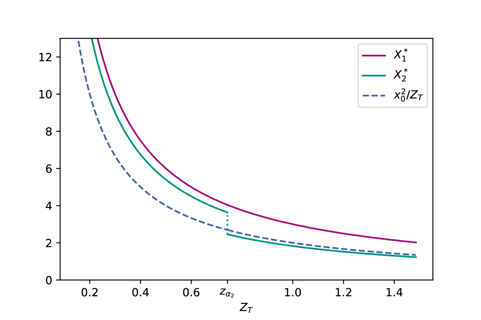
Figure 1. Nash equilibrium $(X_{1}^{*},X_{2}^{*})$ from Theorem 3.3 in terms of $Z_{T}$ for $\alpha_{2}=0.2$, $\beta_{1}=0.9$.

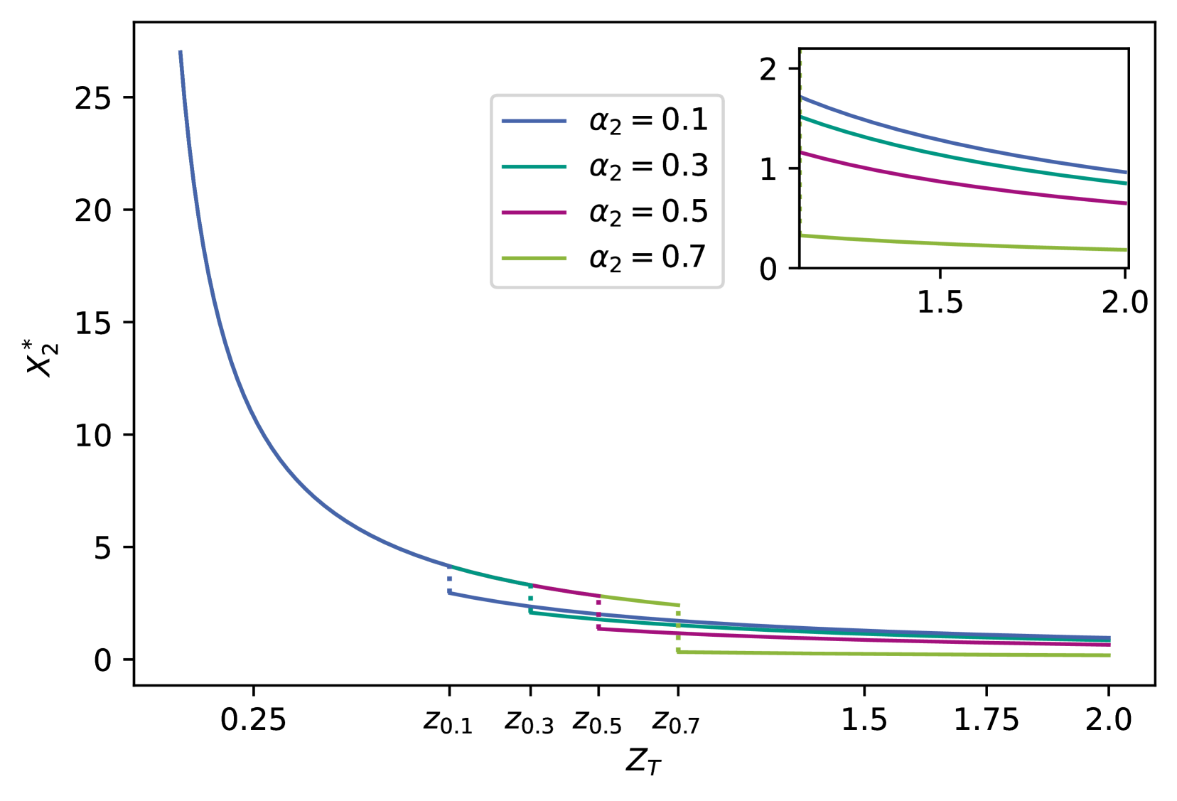
(a) $\beta_{1}=0.9$ and $\alpha_{2}\in\{0.1,0.3,0.5,0.7\}$

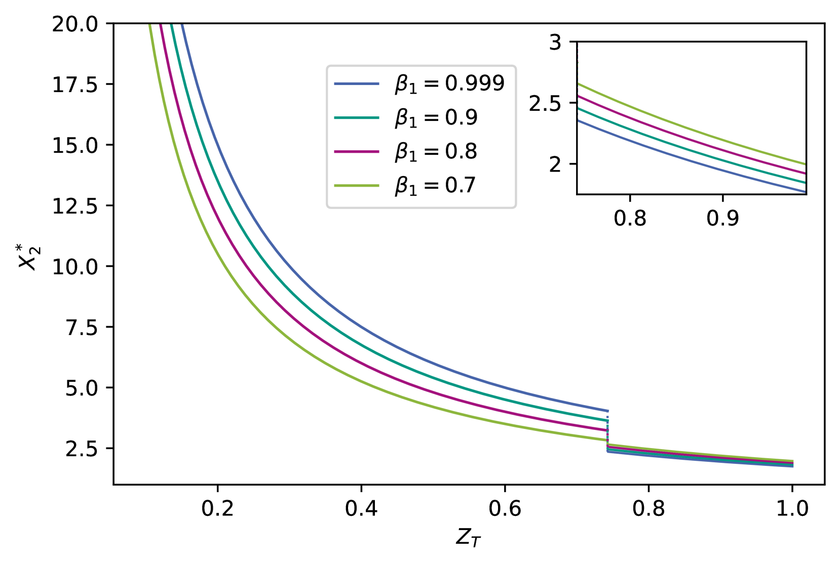
(b) $\alpha_{2}=0.2$ and $\beta_{1}\in\{0.7,0.8,0.9,0.999\}$

Figure 2. Terminal wealth $X_{2}^{*}$ of agent 2 in the Nash equilibrium from Theorem 3.3 in terms of $Z_{T}$ for varying values of $\alpha_{2}$ and $\beta_{1}$.

Figure 2(a) illustrates the influence of the parameter $\alpha_{2}$ on the terminal wealth $X_{2}^{*}$ of agent 2 in the Nash equilibrium. As expected, the location of the discontinuity of $X_{2}^{*}$ is increasing in terms of $\alpha_{2}$ as it is simply given as the $\alpha_{2}$-quantile of $Z_{T}$. Moreover, we notice that for $Z_{T}>z_{\alpha_{2}}$ the value of $X_{2}^{*}$ is decreasing in $\alpha_{2}$. This results from the budget constraint $\mathbb{E}[Z_{T}X_{2}^{*}]=x_{0}^{2}$ since for larger $\alpha_{2}$, the value of $X_{2}^{*}$ is kept on the larger value $\beta_{1}X_{1}^{*}$ on a larger interval.

Figure 2(b) shows the terminal wealth $X_{2}^{*}$ of agent 2 in the Nash equilibrium for different choices of the parameter $\beta_{1}$. We notice a change of order of the value of $X_{2}^{*}$ for the different choices of $\beta_{1}$ located at the discontinuity $z_{\alpha_{2}}.$ For $Z_{T}\leq z_{\alpha_{2}}$, the value of $X_{2}^{*}$ is largest for the largest choice of $\beta_{1}$ as the value of $X_{2}^{*}$ is kept at $\beta_{1}X_{1}^{*}$ in this case. For $Z_{T}>z_{\alpha_{2}}$, the order of the values changes, i.e. the largest choice of $\beta_{1}$ yields the smallest value of $X_{2}^{*}$. This is again due to the budget constraint $\mathbb{E}[Z_{T}X_{2}^{*}]=x_{0}^{2}$.

Finally, let us consider some different possible choices for the set $A_{2}$. As discussed in Remark 3.4, there are infinitely many possible choices for $A_{2}$. Although choosing $A_{2}=\{Z_{T}\leq z_{\alpha_{2}}\}$ maximizes the expected terminal wealth, it is worth considering different choices for $A_{2}$ and their influence on the terminal wealth $X_{2}^{*}$ of agent 2 in the Nash equilibrium. Figure 3 shows $X_{2}^{*}$ for different choices of $A_{2}$ in the form $A_{2}=\{b\leq Z_{T}\leq c\}$. Since $Z_{T}\sim\mathrm{LN}(\nu,\tau)$, for a fixed lower bound $b>0$, the upper bound $c>0$ of the interval is determined via

$$c=\exp\bigg{(}\nu+\tau\cdot\Phi^{-1}\bigg{(}\alpha_{2}+\Phi\bigg{(}\frac{\mathrm{ln}(b)-\nu}{\tau}\bigg{)}\bigg{)}\bigg{)}.$$

Note that the largest possible choice for the lower bound $b$ is the $(1-\alpha_{2})$-quantile of $Z_{T}$, i.e.

$$z_{1-\alpha_{2}}=\exp\left(\nu+\tau\cdot\Phi^{-1}(1-\alpha_{2})\right)\approx 1.2306.$$

We notice that the length of the interval differs significantly depending on whether the interval is located left, right, or around the mode of the distribution of $Z_{T}$.

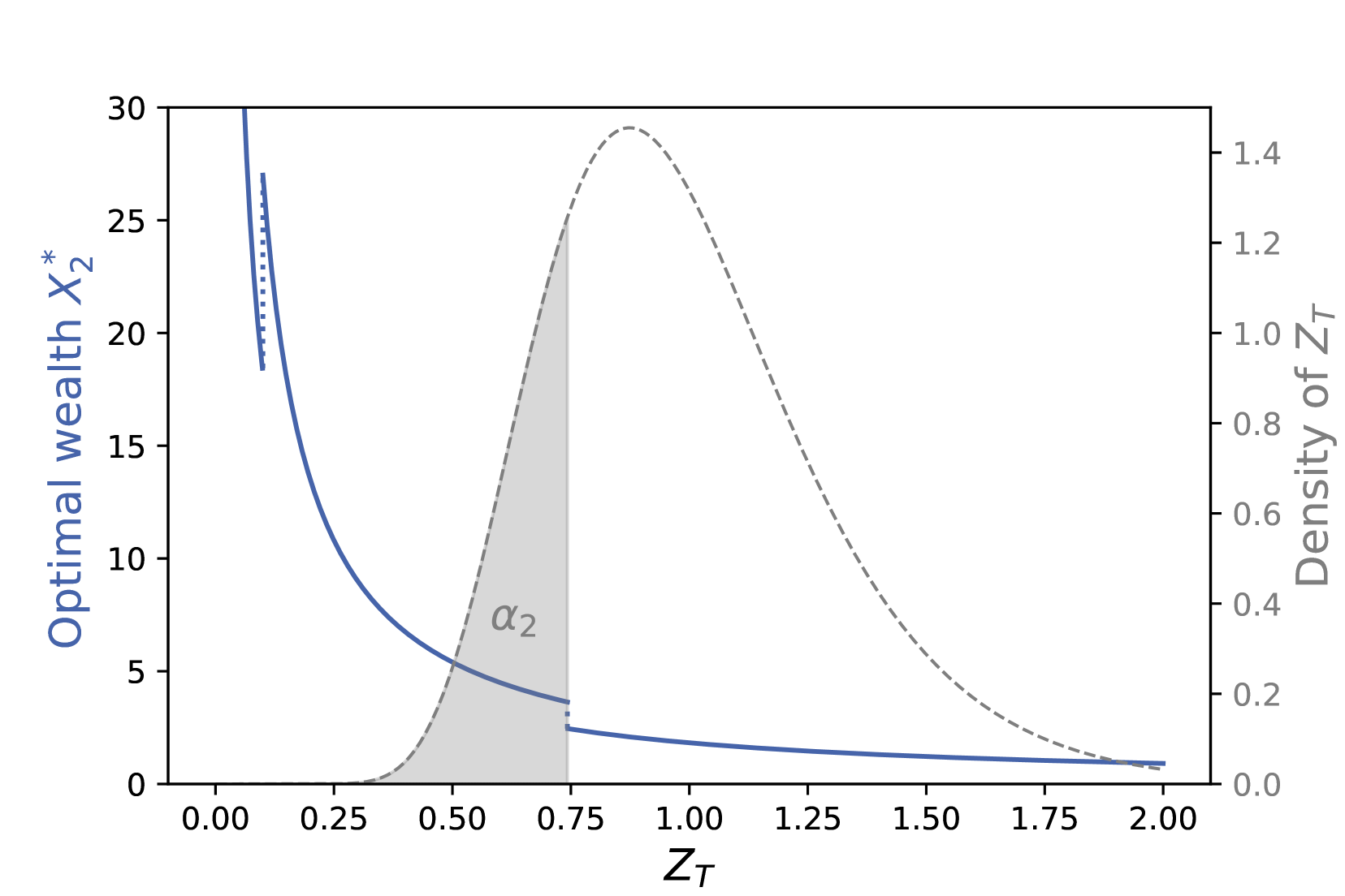
(a) $A_{2}=[0.1,0.7427]$

(b) $A_{2}=[0.5,0.7547]$

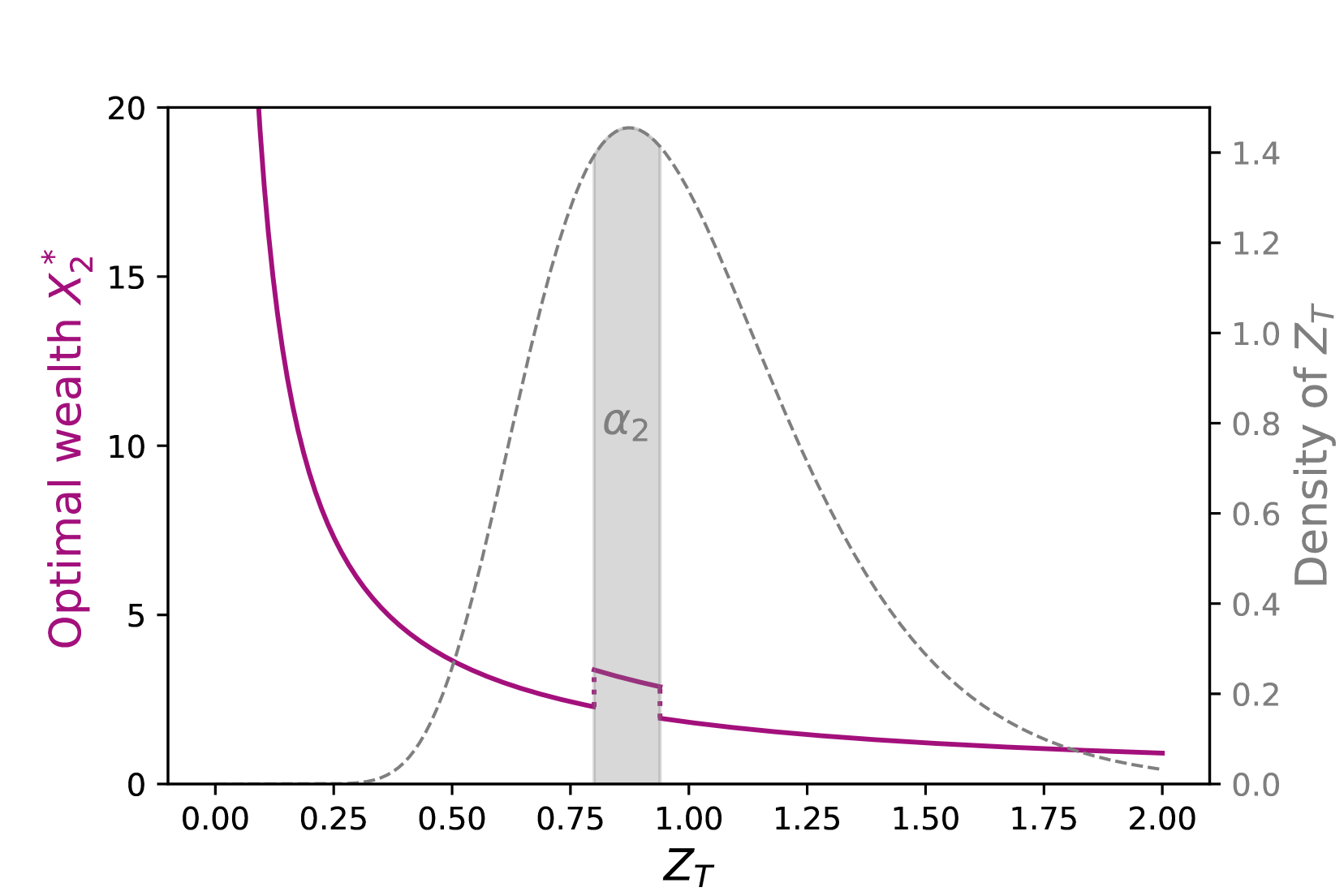
(c) $A_{2}=[0.8,0.9391]$

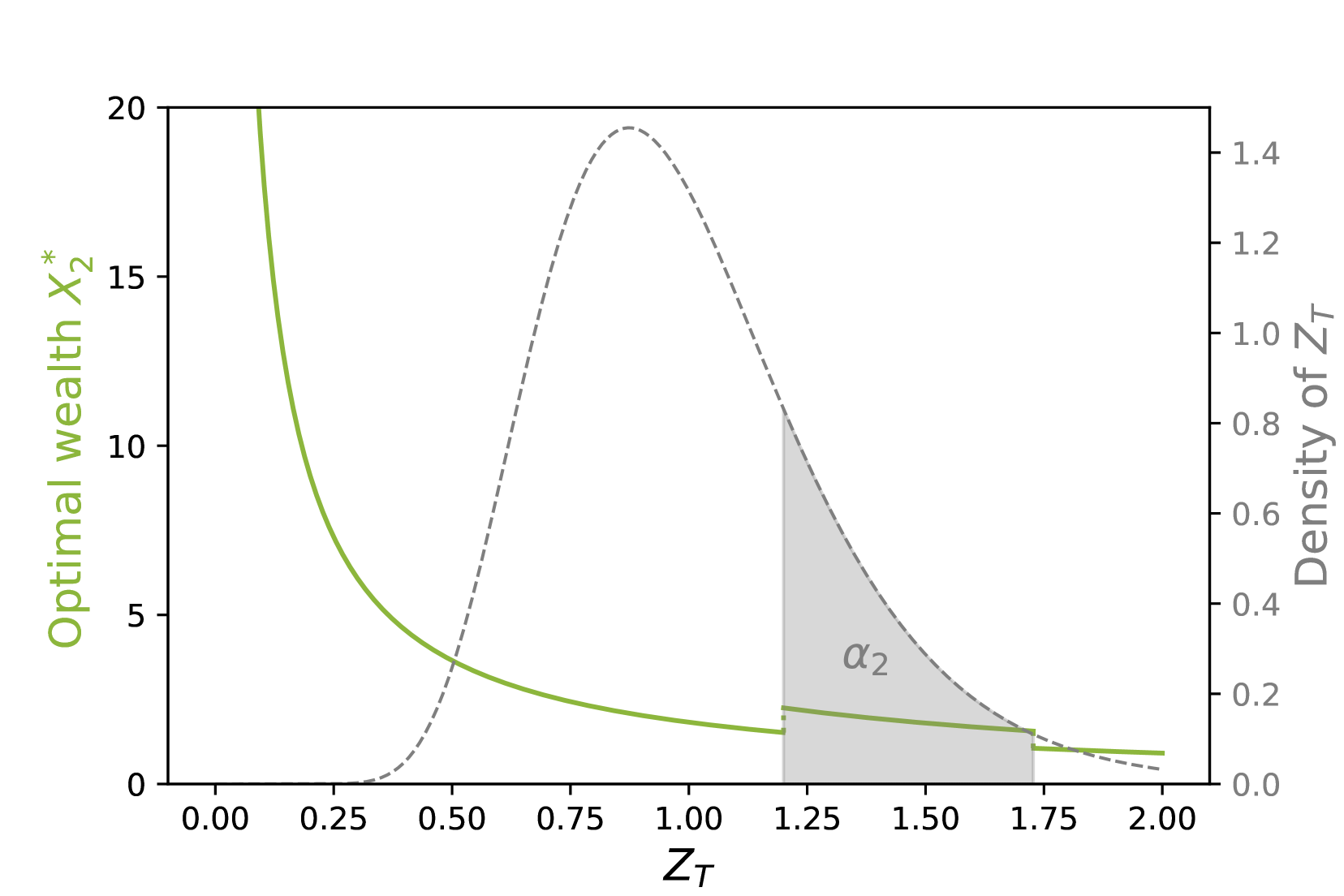
(d) $A_{2}=[1.2,1.7274]$

Figure 3. Terminal wealth $X_{2}^{*}$ of agent 2 in the Nash equilibrium from Theorem 3.3 in terms of $Z_{T}$ for $\beta_{1}=0.9$, $\alpha_{2}=0.2,$ and different choices of the set $A_{2}$.

Next, we consider the Nash equilibrium from Theorem 3.5 in the power case. Since we assumed $Z_{T}$ to be lognormally distributed with parameters $\nu$ and $\tau^{2}$, we can explicitly calculate $\varepsilon_{\gamma}$ and $\mathbb{E}\big{[}Z_{T}^{1-1/\gamma}\mathbbm{1}\{Z_{T}\geq z_{1-\alpha_{2}}\}\big{]}$ to obtain

$$\varepsilon_{\gamma} =\exp\bigg{(}\Big{(}1-\frac{1}{\gamma}\Big{)}\nu+\frac{\tau^{2}}{2}\Big{(}1-\frac{1}{\gamma}\Big{)}^{2}\bigg{)},$$

$$\mathbb{E}\big{[}Z_{T}^{1-1/\gamma}\mathbbm{1}\{Z_{T}\geq z_{1-\alpha_{2}}\}\big{]} =\varepsilon_{\gamma}\Phi\bigg{(}-\frac{\mathrm{ln}(z_{1-\alpha_{2}})-\nu-\tau^{2}(1-1/\gamma)}{\tau}\bigg{)},$$

where $\Phi$ denotes the cumulative distribution function of the standard normal distribution. Figures 4, 5(a) and 5(b) illustrate the Nash equilibrium in terms of $Z_{T}$ for the parameter choice $x_{0}^{1}=3$, $x_{0}^{2}=2$, $\gamma=0.7$ and $\alpha_{i},\beta_{i}$, $i=1,2,$ so that (3.19) holds.

Figure 4 shows the Nash equilibrium $(X_{1}^{*},X_{2}^{*})$ as a function of $Z_{T}$ for $\alpha_{2}=0.5$ and $\beta_{1}=0.9$. The purple and blue solid line show the terminal wealth of agents 1 and 2 in the Nash equilibrium. For comparison, we also illustrated the unconstrained optimal terminal wealth of agent 2 as the green dashed line. Similar to the logarithmic case, the terminal wealth of agent 1 is again the solution to the standard problem without the VaR-based constraint and is thus continuous. The terminal wealth $X_{2}^{*}$ of agent 2 is smaller than the unconstrained terminal wealth for $Z_{T}<z_{1-\alpha_{2}}$ and larger for $Z_{T}\geq z_{1-\alpha_{2}}$ due to the structure of $X_{2}^{*}$ shown in Theorem 3.5.

Figure 5(a) illustrates the influence of the parameter $\alpha_{2}$ on $X_{2}^{*}$. As expected, the location of the discontinuity of $X_{2}^{*}$ is decreasing in terms of $\alpha_{2}$ as it is simply given as the $(1-\alpha_{2})$-quantile of $Z_{T}$. Moreover, we notice that for $Z_{T}<z_{\alpha_{2}}$ the value of $X_{2}^{*}$ is decreasing in $\alpha_{2}$. This results from the budget constraint $\mathbb{E}[Z_{T}X_{2}^{*}]=x_{0}^{2}$ since for larger $\alpha_{2}$, the value of $X_{2}^{*}$ is kept on the larger value $\beta_{1}X_{1}^{*}$ on a larger interval.

Finally, Figure 5(b) shows the terminal wealth $X_{2}^{*}$ of agent 2 in the Nash equilibrium for different choices of the parameter $\beta_{1}$. We notice a change of order of the value of $X_{2}^{*}$ for the different choices of $\beta_{1}$ located at the discontinuity $z_{1-\alpha_{2}}.$ For $Z_{T}\geq z_{1-\alpha_{2}}$, the value of $X_{2}^{*}$ is largest for the largest choice of $\beta_{1}$ as the value of $X_{2}^{*}$ is kept at $\beta_{1}X_{1}^{*}$ in this case. For $Z_{T}<z_{1-\alpha_{2}}$, the order of the values is opposite, i.e. the largest choice of $\beta_{1}$ yields the smallest value of $X_{2}^{*}$. This is again due to the budget constraint $\mathbb{E}[Z_{T}X_{2}^{*}]=x_{0}^{2}$.

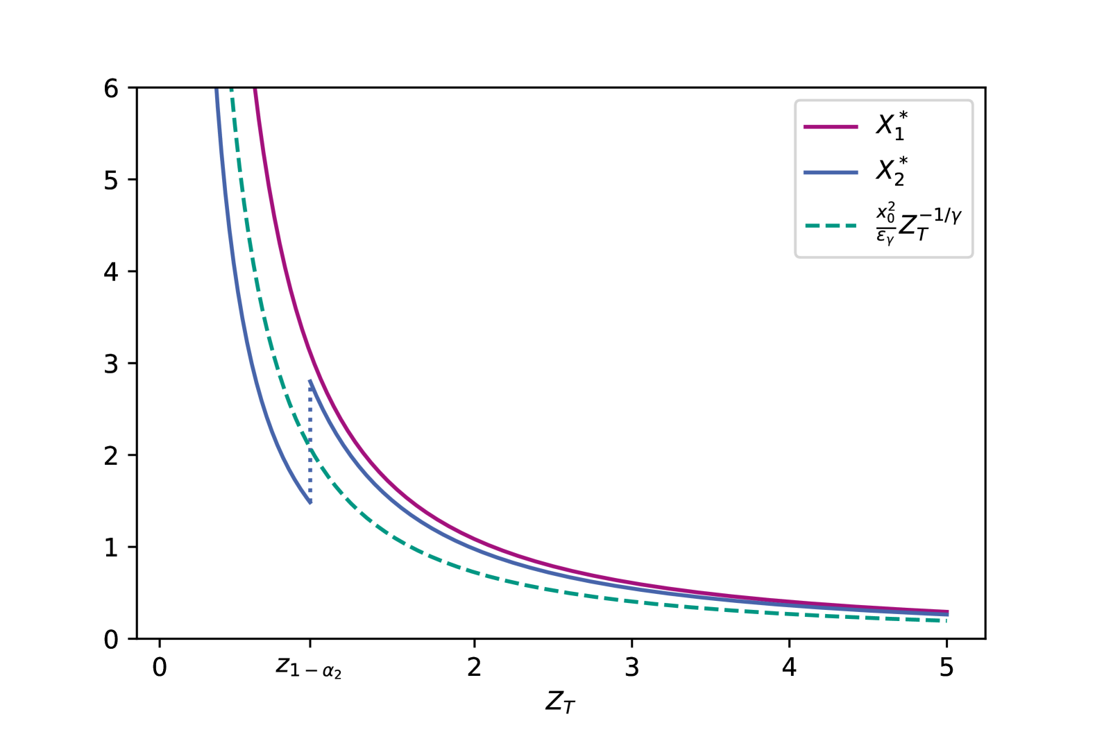
Figure 4. Nash equilibrium $(X_{1}^{*},X_{2}^{*})$ from Theorem 3.5 in terms of $Z_{T}$ for $\alpha_{2}=0.5$, $\beta_{1}=0.9$ and $\gamma=0.7$.

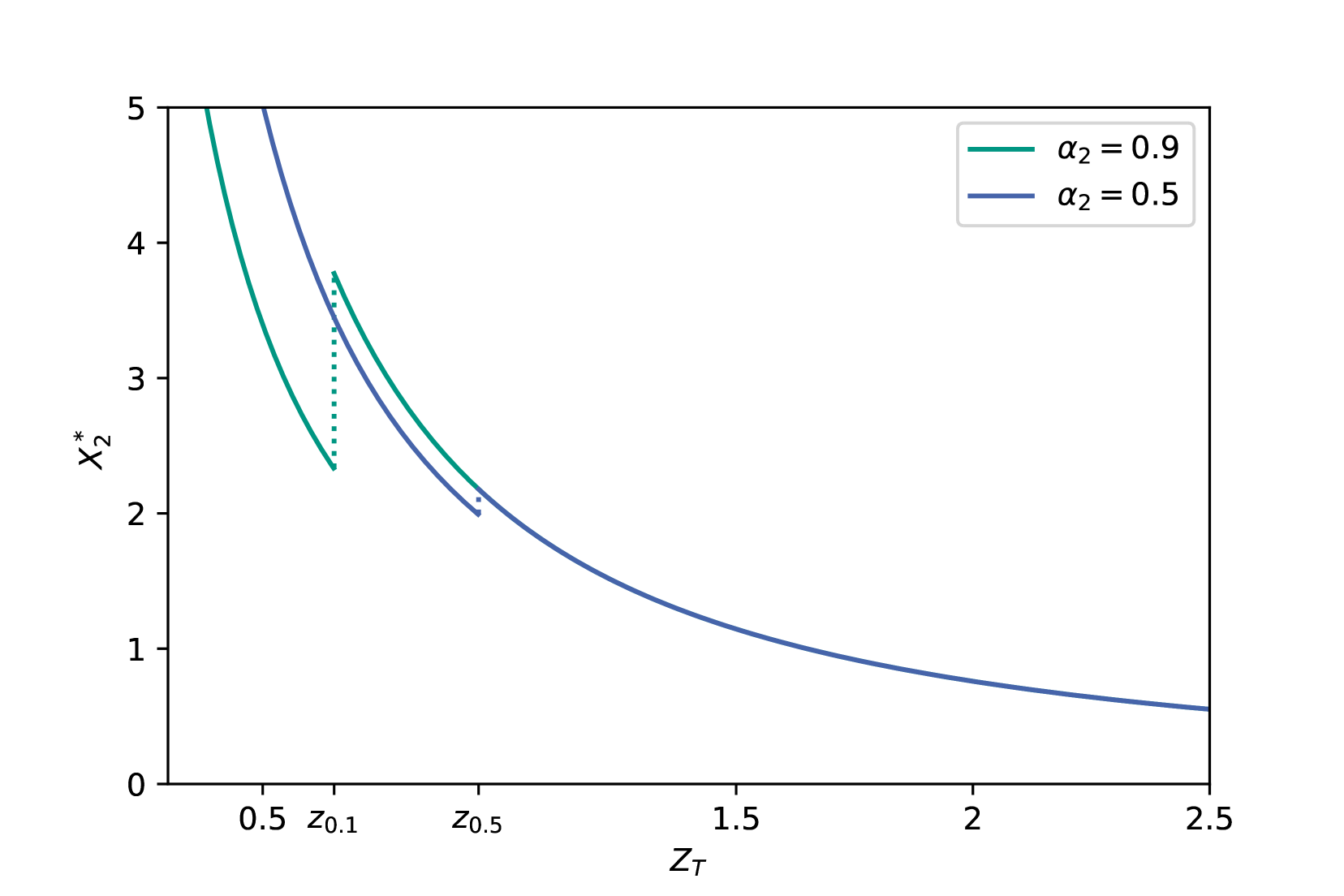
(a) $\beta_{1}=0.9$ and $\alpha_{2}\in\{0.5,0.9\}$

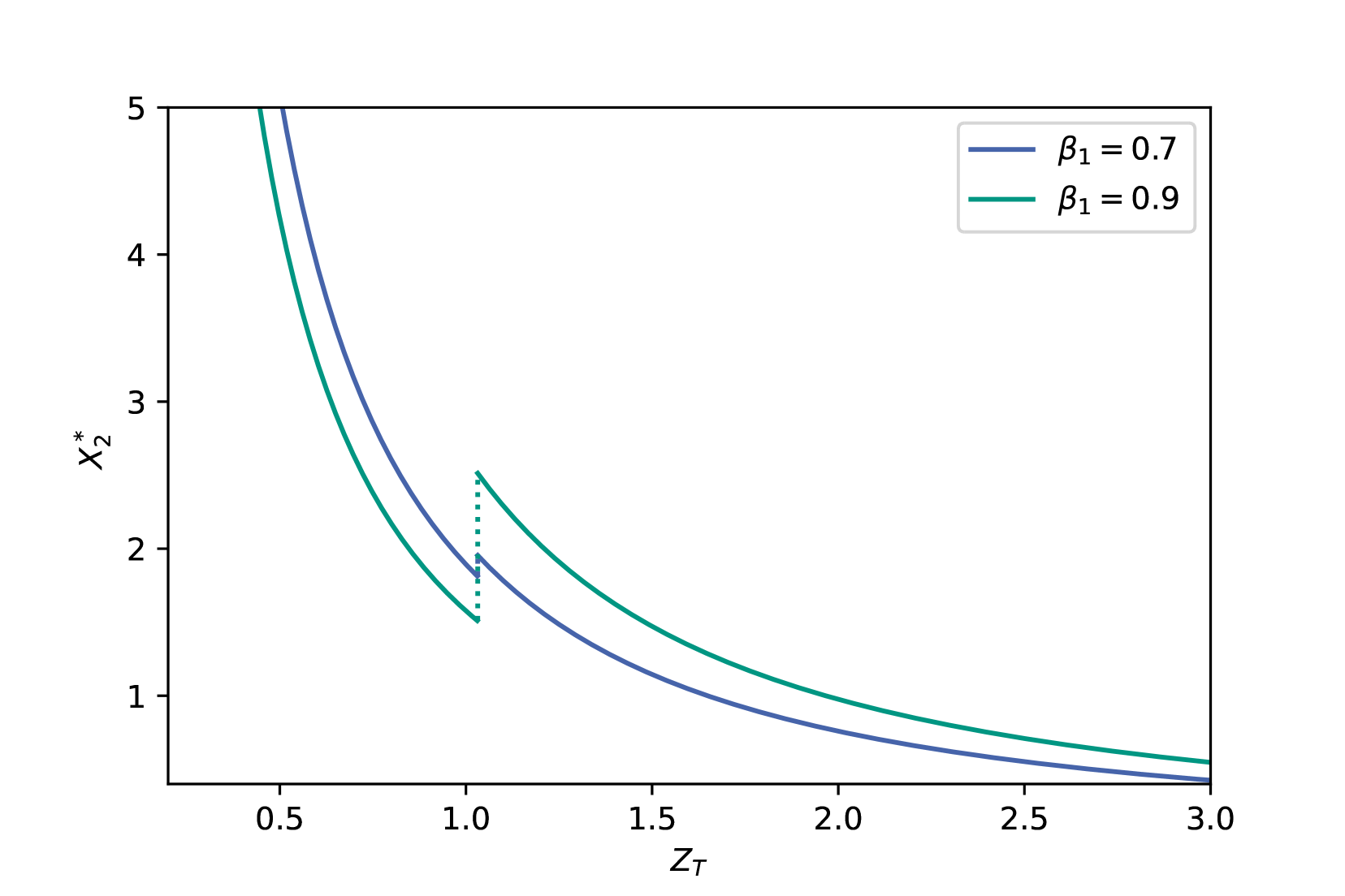
(b) $\alpha_{2}=0.2$ and $\beta_{1}\in\{0.7,0.9\}$

Figure 5. Terminal wealth $X_{2}^{*}$ of agent 2 in the Nash equilibrium from Theorem 3.5 in terms of $Z_{T}$ for $\gamma=0.7$ and different values of $\alpha_{2}$ and $\beta_{1}$.

It remains to discuss Nash equilibria for more than two agents using logarithmic utilities. Here, we restrict to the case that the sum $\alpha_{1}+\ldots+\alpha_{n}$ is less or equal to $1$. Thus, we can use Theorem 4.2 to compute the terminal wealth of the agents in the Nash equilibrium. Figure 6 displays the terminal wealths of $n=4$ agents in the Nash equilibrium for the parameter choice $\alpha_{i}=0.2$, $\beta_{i}=0.3$ for all $i\in\{1,\ldots,4\}$ and $x_{0}^{1}=5$, $x_{0}^{2}=4$, $x_{0}^{3}=3$, $x_{0}^{4}=2$. The sets $A_{i}$, $i=1,\ldots,4,$ are chosen as $A_{i}=(z_{\alpha_{1}+\ldots+\alpha_{i-1}},z_{\alpha_{1}+\ldots+\alpha_{i}}]$, $i=1,\ldots,4$, where $z_{\alpha_{1}+\ldots+\alpha_{i}}:=0$ for $i=0$. We notice that the terminal wealth of agent 4 is larger than the terminal wealth of agent 3 on the set $A_{4}$ although agent 4 starts with a smaller initial capital. However, this results in a terminal wealth on $A_{4}^{c}$ that is significantly smaller than the optimal terminal wealth in the respective unconstrained problems. A comparison of $X_{3}^{*}$ and $X_{4}^{*}$ to the solutions of the respective unconstrained problems can be found in Figures 7(a) and 7(b).

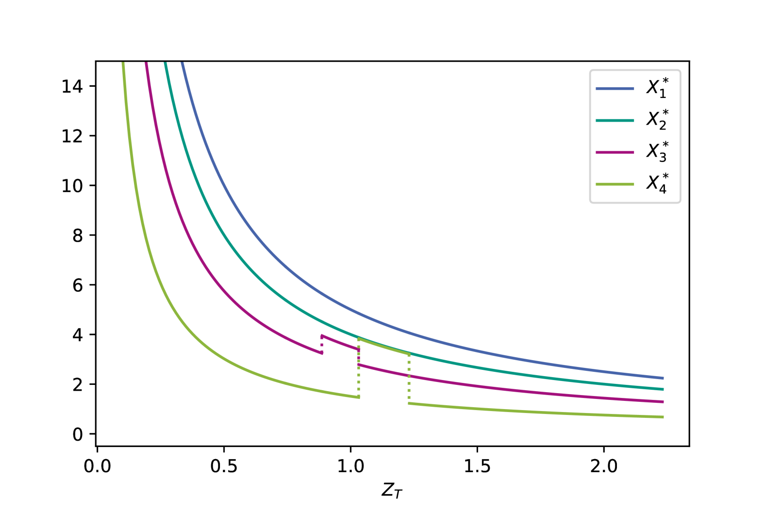
Figure 6. Nash equilibrium $(X_{1}^{*},X_{2}^{*},X_{3}^{*},X_{4}^{*})$ from Theorem 4.2 in terms of $Z_{T}$ for $\alpha_{i}=0.2$, $\beta_{i}=0.3$ for $i\in\{1,\ldots,4\}$, $x_{0}^{1}=5$, $x_{0}^{2}=4$, $x_{0}^{3}=3$, $x_{0}^{4}=2$ and $A_{i}=(z_{\alpha_{1}+\ldots+\alpha_{i-1}},z_{\alpha_{1}+\ldots+\alpha_{i}}]$, $i=1,\ldots,4$, where $z_{\alpha_{1}+\ldots+\alpha_{i}}:=0$ for $i=0$.

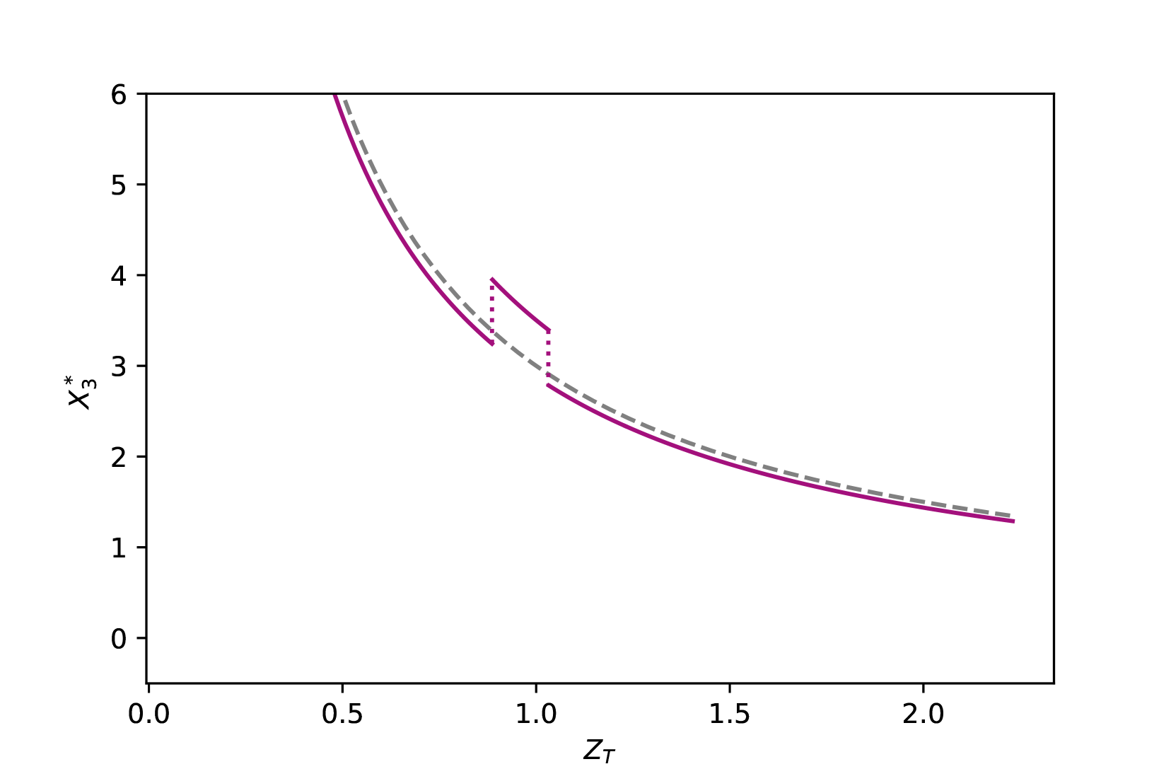
(a) Agent 3

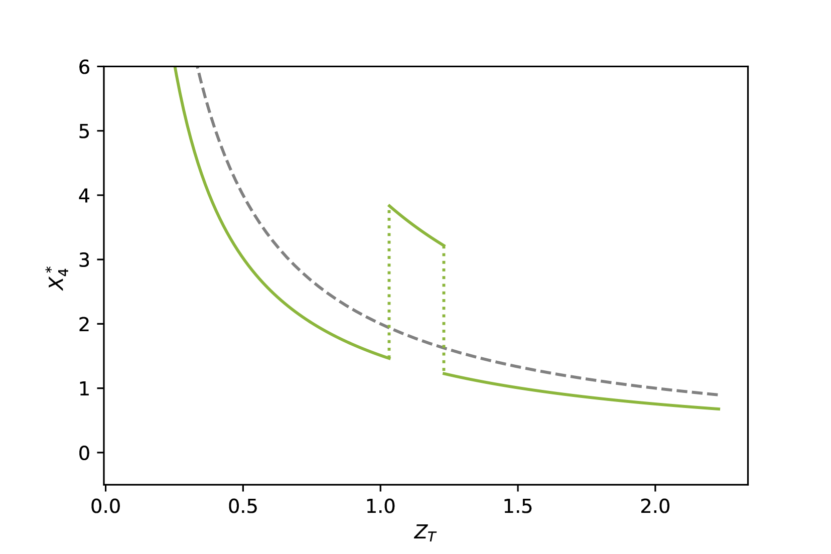
(b) Agent 4

Figure 7. Terminal wealth $X_{j}^{*}$ of agents $j$, $j\in\{3,4\},$ in the Nash equilibrium from Theorem 4.2 (solid) and the associated optimal terminal wealth in the unconstrained problem (dashed) in terms of $Z_{T}$.

7. Conclusion

It is meaningful to consider competing agents by introducing probability constraints instead of relative wealth targets. However, it turns out that finding Nash equilibria is in general more challenging. An interesting case which is analytically solvable is the case that all investors have a logarithmic utility function. In this case, Nash equilibria (if they exist) can be found for an arbitrary number of agents. In order to succeed, a number of parameter cases have to be distinguished leading either to no Nash equilibrium, a unique Nash equilibrium or an infinite number of Nash equilibria. We illustrate our findings by numerical examples. For other utility functions, and in particular, if the agents have different utility functions, the problem is much more demanding and we leave it for future research.

8. Appendix

8.1. Utility maximization with lower bounds I

Suppose $Y\geq 0$ is an arbitrary $\mathcal{F}-$measurable random variable, $U:[0,\infty)\to\mathbb{R}$ a strictly increasing, strictly concave and differentiable utility. We want to solve the following problem

$$(P_{Y})\left\{\begin{array}[]{l}\mathbb{E}U(X)\to\max\\ X\geq Y,\;X\mbox{ is }\mathcal{F}-\mbox{measurable,}\\ \mathbb{E}[Z_{T}X]=x_{0}.\end{array}\right.$$

Obviously $x_{0}\geq\mathbb{E}[Z_{T}Y]$ since otherwise it is not possible to fulfill the constraint. We claim that the optimal solution is given as follows (cp. El Karoui et al., (2005), Prop. 2.2 for a special case).

Lemma 8.1.

The optimal solution of problem $(P_{Y})$ is given by

$$X^{*}=\max\Big{\{}Y,I(\lambda Z_{T})\Big{\}},$$

where $\lambda>0$ is such that $\mathbb{E}[Z_{T}X^{*}]=x_{0}$ and $I$ is the inverse function of $U^{\prime}.$ It is the unique solution up to sets of measure zero.

Proof.

Obviously $X^{*}$ is admissible for $(P_{Y})$. In order to show optimality, let $X$ be another feasible random variable. Since $U$ is concave and differentiable it holds that

$$U(X)\leq U(X^{*})+U^{\prime}(X^{*})(X-X^{*}).$$

Now we have to show $\mathbb{E}[U^{\prime}(X^{*})(X-X^{*})]\leq 0.$ Let $A:=\{X^{*}=I(\lambda Z_{T})\}.$ Observe first that

$$U^{\prime}(X^{*})=\mathbbm{1}_{A}U^{\prime}(I(\lambda Z_{T}))+\mathbbm{1}_{A^{c}}U^{\prime}(Y)=\mathbbm{1}_{A}\lambda Z_{T}+\mathbbm{1}_{A^{c}}U^{\prime}(Y).$$

Thus, we obtain

$$U^{\prime}(X^{*})(X-X^{*}) =\left[\mathbbm{1}_{A}\lambda Z_{T}+\mathbbm{1}_{A^{c}}U^{\prime}(Y)\right](X-X^{*})$$

$$=\lambda{Z_{T}}(X-X^{*})+\mathbbm{1}_{A^{c}}\big{(}U^{\prime}(Y)-\lambda Z_{T}\big{)}(X-X^{*})$$

$$=\lambda{Z_{T}}(X-X^{*})+\mathbbm{1}_{A^{c}}\big{(}U^{\prime}(Y)-\lambda Z_{T}\big{)}(X-Y).$$

The last equation is true since on $A^{c}$ we have $X^{*}=Y.$ Now we take the expectation on both sides. Since $X$ and $X^{*}$ are both feasible we have $\mathbb{E}[Z_{T}(X-X^{*})]=x_{0}-x_{0}=0.$ Thus

$$\mathbb{E}[U^{\prime}(X^{*})(X-X^{*})]=\mathbb{E}\left[\mathbbm{1}_{A^{c}}\big{(}U^{\prime}(Y)-\lambda Z_{T}\big{)}(X-Y)\right]\leq 0.$$

The inequality is true since $X\geq Y$ and

$$U^{\prime}(Y)\leq\lambda Z_{T}\Leftrightarrow Y\geq I(\lambda Z_{T})$$

which is true on $A^{c}.$ Finally we show uniqueness. Suppose that both $X^{*}$ and $\tilde{X}$ are optimal, i.e. $\mathbb{E}U(X^{*})=\mathbb{E}U(\tilde{X})$ and both are admissible. Consider $X:=\alpha X^{*}+(1-\alpha)\tilde{X}$ for $\alpha\in(0,1).$ Obviously $X$ is again admissible and

$$\mathbb{E}U(X)>\alpha\mathbb{E}U(X^{*})+(1-\alpha)\mathbb{E}U(\tilde{X})$$

as long as $X^{*}$ and $\tilde{X}$ do not coincide outside a set of measure zero, which leads to the contradiction that $X$ attains a higher value. ∎

If $U(x)=\ln(x)$ we obtain $I(x)=1/x.$ Thus, with a slight misuse of the parameter $\lambda$ (instead of $\lambda$ we rather consider $1/\lambda$), we obtain in the situation of Lemma 8.1 that $X^{*}=\max\Big{\{}Y,\lambda/Z_{T}\Big{\}}$ where $\lambda$ is such that $\mathbb{E}[Z_{T}X^{*}]=x_{0}$.

8.2. Utility maximization with lower bounds II

Now we consider the problem with logarithmic utility where the constraint only has to be satisfied on a subset of $\Omega.$ We assume here that $Y>0.$ Then the optimization problem reads as

$$(P_{A})\left\{\begin{array}[]{l}\mathbb{E}\ln(X)\to\max\\ X\geq Y\mathbbm{1}_{A},\;X\mbox{ is }\mathcal{F}-\mbox{measurable},A\in\mathcal{F},\\ \mathbb{P}(A)=\alpha,\\ \mathbb{E}[Z_{T}X]=x_{0}.\end{array}\right.$$

Note that the optimization is over $X$ and the set $A$ here. Obviously, $x_{0}\geq\mathbb{E}[Z_{T}Y\mathbbm{1}_{A}]$ has to be fulfilled for an $A\in\mathcal{F}$, otherwise it is not possible to fulfill the constraint. Let us define

$$M_{\lambda}:=\{Y\leq\lambda/Z_{T}\}$$

and let $\lambda_{\alpha}:=\inf\{\lambda:\mathbb{P}(M_{\lambda})\geq\alpha\}.$ Note that if $\lambda_{\alpha}\leq x_{0}$ then the problem is trivial and the optimal solution is given by $X^{*}=x_{0}/Z_{T}.$

Lemma 8.2.

The optimal solution of problem $(P_{A})$ is given by

$$X^{*}=\mathbbm{1}_{M_{\lambda_{\alpha}}}\max\Big{\{}Y,\lambda/Z_{T}\Big{\}}+\mathbbm{1}_{M_{\lambda_{\alpha}}^{c}}\lambda/Z_{T}$$

where $\lambda$ is such that $\mathbb{E}[Z_{T}X^{*}]=x_{0}$.

Proof.

First it is slightly more convenient to transform the random variables as follows. Define

$$\tilde{Y}:=YZ_{T},\mbox{ and }\tilde{X}:=XZ_{T}.$$ (8.1)

Then, instead of $(P_{A})$ we can consider

$$(\tilde{P}_{A})\left\{\begin{array}[]{l}\mathbb{E}\ln(\tilde{X})\to\max\\ \tilde{X}\geq\tilde{Y}\mathbbm{1}_{A},\;\tilde{X}\mbox{ is }\mathcal{F}-\mbox{measurable},A\in\mathcal{F},\\ \mathbb{P}(A)=\alpha,\\ \mathbb{E}[\tilde{X}]=x_{0}.\end{array}\right.$$

We begin with the special case that $\tilde{Y}$ is discrete and has finitely many different values, i.e.

$$\tilde{Y}=\sum_{k=1}^{m}y_{k}1_{A_{k}}$$

for a partition $(A_{k})_{k=1,\ldots,m}$ of $\Omega.$ Suppose $\tilde{X}$ is admissible for $(\tilde{P}_{A})$ and define $\tilde{A}:=\{\tilde{X}\geq\tilde{Y}\}$. Since $\tilde{X}$ is admissible we must have $\mathbb{P}(\tilde{A})\geq\alpha.$ Further let

$$B_{k}:=A_{k}\cap\tilde{A},\quad C_{k}:=A_{k}\cap\tilde{A}^{c}.$$ (8.2)

I.e. we split the sets $A_{k}$ where $\tilde{Y}$ is constant into those parts where $\tilde{X}\geq\tilde{Y}$ and those where $\tilde{X}<\tilde{Y}$. We define now a new random variable $\hat{X}$ by

$$\hat{X}:=\sum_{k=1}^{m}x_{k}^{1}1_{B_{k}}+\sum_{k=1}^{m}x_{k}^{2}1_{C_{k}},$$ (8.3)

where

$$x_{k}^{1}:=\frac{1}{\mathbb{P}(B_{k})}\int_{B_{k}}\tilde{X}d\mathbb{P},\quad x_{k}^{2}:=\frac{1}{\mathbb{P}(C_{k})}\int_{C_{k}}\tilde{X}d\mathbb{P}.$$ (8.4)

This means we replace $\tilde{X}$ on the sets $B_{k},C_{k}$ by the corresponding expectation. Note that $\hat{X}$ is again admissible for $(\tilde{P}_{A})$ since on $B_{k}$ we have $\tilde{X}\geq y_{k}$ and thus $x_{k}^{1}\geq y_{k}.$ Moreover, we obtain that $\mathbb{E}\ln(\hat{X})\geq\mathbb{E}\ln(\tilde{X})$ because due to the Jensen inequality we have (we denote by $\mathbb{P}_{B_{k}}$ the conditional probability of $\mathbb{P}$ given $B_{k}$, i.e. $\mathbb{P}_{B_{k}}(D)=\mathbb{P}(D\cap B_{k})/\mathbb{P}(B_{k})$) that

$$\int_{B_{k}}\ln(\tilde{X})d\mathbb{P} =\mathbb{P}(B_{k})\int\ln(\tilde{X})d\mathbb{P}_{B_{k}}\leq\mathbb{P}(B_{k})\ln\Big{(}\int\tilde{X}d\mathbb{P}_{B_{k}}\Big{)}=\mathbb{P}(B_{k})\ln(x_{k}^{1})$$ (8.5)

and the same for the sets $C_{k}$. Summing up these integrals we see that the expected utility of $\hat{X}$ is not less than the expected utility for $\tilde{X}.$ Thus, we can restrict the optimization to random variables $\hat{X}$ which are discrete and have finitely many positive values.

Fix an admissible discrete $\hat{X}$ and assume that there exists a measurable set $F\subset B_{k}$ for an arbitrary $k$ and a measurable set $\tilde{F}\subset C_{j}$ for $j\neq k$ and with $\mathbb{P}(F)=\mathbb{P}(\tilde{F})>0$ such that $y_{k}>y_{j}.$ Note that $\mathbb{P}(F)$ may be arbitrary small. This means that the constraint is satisfied on a larger level $y_{k}$ whereas it is not satisfied on a smaller level $y_{j}.$ By construction, the random variable $\hat{X}$ takes value $x_{k}^{1}$ on set $B_{k}$ and value $x_{j}^{2}$ on $C_{j}.$ Thus we have

$$x_{j}^{2}<y_{j}<y_{k}\leq x_{k}^{1}.$$

Now define the random variable

$$X^{*}:=\hat{X}\mathbbm{1}_{(F\cup\tilde{F})^{c}}+y_{j}\mathbbm{1}_{\tilde{F}}+(x_{j}^{2}+x_{k}^{1}-y_{j})\mathbbm{1}_{F}.$$

Note that $x_{j}^{2}+x_{k}^{1}-y_{j}>0$ and $\mathbb{E}\hat{X}=\mathbb{E}X^{*}.$ Moreover, $X^{*}$ also satisfies the constraint due to our construction. Let us consider the difference in expected utility of $\hat{X}$ and $X^{*}:$

$$\mathbb{E}\ln(X^{*})-\mathbb{E}\ln(\hat{X})=\mathbb{P}(F)\Big{(}\ln(y_{j})+\ln(x_{j}^{2}+x_{k}^{1}-y_{j})-\ln(x_{k}^{1})-\ln(x_{j}^{2})\Big{)}>0.$$ (8.6)

The latter inequality follows since $\mathbb{R}^{m}\ni(x_{1},\ldots,x_{m})\mapsto\sum_{k=1}^{m}\ln(x_{k})$ is Schur-concave (see Marshall and Olkin, (1979), Chapt.1, Sec. A). Thus, we obtain that it is always better to satisfy the constraint on a set where $Y$ takes the smallest values. This implies the statement for discrete $Y$. In order to show the statement for arbitrary $Y$, approximate $Y$ by a sequence of discrete $(Y_{n})$ almost surely. Taking the limit $n\to\infty$ then implies the general result. ∎

8.3. Maximizing $L$

Recall that

$$L(X,\lambda_{2},\eta_{2}):=U(X)-\lambda_{2}Z_{T}X+\eta_{2}\mathbbm{1}_{[X\geq\beta_{1}I(\lambda_{1}Z_{T})]}$$

with $\lambda_{2},\eta_{2}\geq 0$ fixed. We show that $L$ is maximized by $X_{2}^{*}$ from (3.20). Obviously the maximum points can either be $I(\lambda_{2}Z_{T})$ or $\beta_{1}I(\lambda_{1}Z_{T})$ where $I(\lambda_{2}Z_{T})<\beta_{1}I(\lambda_{1}Z_{T}).$ We can compare the two possible values of the function $L$:

$$F(Z_{T}):=U(I(\lambda_{2}Z_{T}))-\lambda_{2}Z_{T}I(\lambda_{2}Z_{T})-\Big{\{}U(\beta_{1}I(\lambda_{1}Z_{T}))-\lambda_{2}Z_{T}\beta_{1}I(\lambda_{1}Z_{T})+\eta_{2}\Big{\}}.$$

Differentiating $F$ yields

$$F^{\prime}(Z_{T}) =\lambda_{2}\big{(}\beta_{1}I(\lambda_{1}Z_{T})-I(\lambda_{2}Z_{T})\big{)}-\beta_{1}\lambda_{1}Z_{T}I^{\prime}(\lambda_{1}Z_{T})(\lambda_{1}\beta_{1}^{-\gamma}-\lambda_{2})$$

$$=Z_{T}^{-1/\gamma}\bigg{(}\lambda_{2}\Big{(}\beta_{1}\lambda_{1}^{-1/\gamma}-\lambda_{2}^{-1/\gamma}\Big{)}+\frac{\beta_{1}\lambda_{1}^{-1/\gamma}}{\gamma}\Big{(}\lambda_{1}\beta_{1}^{-\gamma}-\lambda_{2}\Big{)}\bigg{)}=:Z_{T}^{-1/\gamma}f(\lambda_{2}).$$

Since $Z_{T}>0$, it suffices to consider the sign of $f(\lambda_{2})$ to discuss the monotonicity of $F$. We observe that

$$f\big{(}\lambda_{1}\beta_{1}^{-\gamma}\big{)}=0.$$

Moreover, differentiating $f$ yields

$$f^{\prime}(\lambda_{2}) =\Big{(}1-1/\gamma\Big{)}\Big{(}\beta_{1}\lambda_{1}^{-1/\gamma}-\lambda_{2}^{-1/\gamma}\Big{)},$$

so that $f^{\prime}(\lambda_{2})<0$ for all $\lambda_{2}>\lambda_{1}\beta_{1}^{-\gamma}$. Thus, since we already saw in the proof of Theorem 3.5 that $\lambda_{2}>\lambda_{1}\beta_{1}^{-\gamma}$, we deduce that $F^{\prime}(Z_{T})<0$ for all values of $Z_{T}$. Moreover, by definition of $\eta_{2}$, we have $F(z_{1-\alpha_{2}})=0$ which implies that $X_{2}^{*}$ maximizes the function $L$.

References

- Anthropelos et al., (2022) Anthropelos, M., Geng, T., and Zariphopoulou, T. (2022). Competition in fund management and forward relative performance criteria. SIAM Journal on Financial Mathematics, 13(4):1271–1301.
- Aydoğan and Steffensen, (2024) Aydoğan, B. and Steffensen, M. (2024). Optimal investment strategies under the relative performance in jump-diffusion markets. Decisions in Economics and Finance, pages 1–26.
- Basak and Makarov, (2014) Basak, S. and Makarov, D. (2014). Strategic asset allocation in money management. The Journal of finance, 69(1):179–217.
- Basak and Makarov, (2015) Basak, S. and Makarov, D. (2015). Competition among portfolio managers and asset specialization. Paris December 2014, Finance Meeting EUROFIDAI-AFFI Paper.
- Basak and Shapiro, (2001) Basak, S. and Shapiro, A. (2001). Value-at-risk-based risk management: Optimal policies and asset prices. The review of financial studies, 14(2):371–405.
- Bäuerle and Chen, (2023) Bäuerle, N. and Chen, A. (2023). Optimal investment under partial information and robust var-type constraint. International Journal of Theoretical and Applied Finance, 26(4-5).
- Bäuerle and Göll, (2023) Bäuerle, N. and Göll, T. (2023). Nash equilibria for relative investors via no-arbitrage arguments. Mathematical Methods of Operations Research, 97(1):1–23.
- Bäuerle and Göll, (2024) Bäuerle, N. and Göll, T. (2024). Nash equilibria for relative investors with (non) linear price impact. Mathematics and Financial Economics, pages 1–22.
- Bell and Cover, (1980) Bell, R. M. and Cover, T. M. (1980). Competitive optimality of logarithmic investment. Mathematics of Operations Research, 5(2):161–166.
- Brown et al., (2001) Brown, S. J., Goetzmann, W. N., and Park, J. (2001). Careers and survival: Competition and risk in the hedge fund and CTA industry. The Journal of Finance, 56(5):1869–1886.
- Browne, (1999) Browne, S. (1999). Reaching goals by a deadline: Digital options and continuous-time active portfolio management. Advances in Applied Probability, 31(2):551–577.
- Curatola, (2024) Curatola, G. (2024). Asset prices when large investors interact strategically. Quantitative Finance, pages 1–18.
- Dos Reis and Platonov, (2021) Dos Reis, G. and Platonov, V. (2021). Forward utilities and mean-field games under relative performance concerns. In Bernardin, C., Golse, F., Gonçalves, P., Ricci, V., and Soares, A. J., editors, From Particle Systems to Partial Differential Equations: International Conference, Particle Systems and PDEs VI, VII and VIII, 2017-2019, volume 352, pages 227–251, Cham. Springer.
- El Karoui et al., (2005) El Karoui, N., Jeanblanc, M., and Lacoste, V. (2005). Optimal portfolio management with american capital guarantee. Journal of Economic Dynamics and Control, 29(3):449–468.
- Espinosa, (2010) Espinosa, G.-E. (2010). Stochastic Control Methods for Optimal Portfolio Investment. PhD thesis, Ecole Polytechnique Paris.
- Espinosa and Touzi, (2015) Espinosa, G.-E. and Touzi, N. (2015). Optimal investment under relative performance concerns. Mathematical Finance, 25(2):221–257.
- Föllmer and Schied, (2016) Föllmer, H. and Schied, A. (2016). Stochastic Finance: An Introduction in Discrete Time. Walter de Gruyter, Berlin/Boston, 4. edition.
- Fu, (2023) Fu, G. (2023). Mean field portfolio games with consumption. Mathematics and Financial Economics, 17(1):79–99.
- Fu and Zhou, (2023) Fu, G. and Zhou, C. (2023). Mean field portfolio games. Finance and Stochastics, 27(1):189–231.
- Gabih et al., (2006) Gabih, A., Grecksch, W., Richter, M., and Wunderlich, R. (2006). Optimal portfolio strategies benchmarking the stock market. Mathematical Methods of Operations Research, 64:211–225.
- Gabih et al., (2005) Gabih, A., Grecksch, W., and Wunderlich, R. (2005). Dynamic portfolio optimization with bounded shortfall risks. Stochastic analysis and applications, 23(3):579–594.
- Gabih et al., (2009) Gabih, A., Sass, J., and Wunderlich, R. (2009). Utility maximization under bounded expected loss. Stochastic Models, 25(3):375–407.
- Hu and Zariphopoulou, (2022) Hu, R. and Zariphopoulou, T. (2022). -player and mean-field games in Itô-diffusion markets with competitive or homophilous interaction. In Stochastic Analysis, Filtering, and Stochastic Optimization. Springer, Cham.
- Kempf and Ruenzi, (2008) Kempf, A. and Ruenzi, S. (2008). Tournaments in mutual-fund families. The Review of Financial Studies, 21(2):1013–1036.
- Korn and Korn, (2013) Korn, R. and Korn, E. (2013). Optionsbewertung und Portfolio-Optimierung: Moderne Methoden der Finanzmathematik. Springer-Verlag.
- Korn and Lindberg, (2014) Korn, R. and Lindberg, C. (2014). Portfolio optimization for an investor with a benchmark. Decisions in Economics and Finance, 37:373–384.
- Kovenock and Roberson, (2021) Kovenock, D. and Roberson, B. (2021). Generalizations of the general lotto and Colonel Blotto games. Economic Theory, 71:997–1032.
- Kraft et al., (2020) Kraft, H., Meyer-Wehmann, A., and Seifried, F. T. (2020). Dynamic asset allocation with relative wealth concerns in incomplete markets. Journal of Economic Dynamics and Control, 113:103857.
- Lacker and Soret, (2020) Lacker, D. and Soret, A. (2020). Many-player games of optimal consumption and investment under relative performance criteria. Mathematics and Financial Economics, 14(2):263–281.
- Lacker and Zariphopoulou, (2019) Lacker, D. and Zariphopoulou, T. (2019). Mean field and -agent games for optimal investment under relative performance criteria. Mathematical Finance, 29(4):1003–1038.
- Marshall and Olkin, (1979) Marshall, A. and Olkin, I. (1979). Inequalities: Theory of Majorization and Its Applications. Academic Press, Inc.
- Musiela and Zariphopoulou, (2006) Musiela, M. and Zariphopoulou, T. (2006). Investments and forward utilities. preprint.
- Sass and Wunderlich, (2010) Sass, J. and Wunderlich, R. (2010). Optimal portfolio policies under bounded expected loss and partial information. Mathematical Methods of Operations Research, 72:25–61.