Two-mode Floquet quantum master approach for quantum transport through mesoscopic systems: Engineering of the fractional quantization

Abstract

Simultaneous driving by two periodic oscillations yields a practical technique for further engineering quantum systems. For quantum transport through mesoscopic systems driven by two strong periodic terms, a non-perturbative Floquet-based quantum master equation (QME) approach is developed using a set of dissipative time-dependent terms and the reduced density matrix of the system. This work extends our previous Floquet approach for transport through quantum dots (at finite temperature and arbitrary bias) driven periodically by a single frequency. In a pedagogical way, we derive explicit time-dependent dissipative terms. Our theory begins with the derivation of the two-mode Floquet Liouville-von Neumann equation. We then explain the second-order Wangsness-Bloch-Redfield QME with a slightly modified definition of the interaction picture. Subsequently, the two-mode Shirley time evolution formula is applied, allowing for the integration of reservoir dynamics. Consequently, the established formalism has a wide range of applications in open quantum systems driven by two modes in the weak coupling regime. The formalism’s potential applications are demonstrated through various examples.

I Introduction

Quantum transport through mesoscopic nanostructures exhibits a range of remarkable static characteristics, including quantized conductance [1, 2, 3], Coulomb blockade [4], quantum interference [5, 6, 7], Kondo effect [8, 9], and spin filtering [10]. Meanwhile, dynamic effects such as quantum coherence, polaron formation [11, 12, 13], molecular vibronic coupling [14], etc., have attracted interest in the solid-state physics and quantum chemistry communities. Dynamical control, for example, by applying oscillating fields to the original systems, allows for the discovery of new properties unattainable by only altering static experimental conditions. Very recently, there has been an increasing interest in controlling the dynamics of quantum systems or chemical reactions by driving the system with more than only one frequency, which may described as multi-mode Floquet engineering [15, 16, 17, 18, 19, 20]. For instance, mediated by the strong spin-orbit interactions in a hole silicon spin qubits, the proposed phase-driving technique couples a secondary frequency (radio wave) to the qubit phase to reduce the susceptibility of the qubit to the noise [21]. To the best of our knowledge, there are no theoretical quantum transport reports (on open quantum systems) where the dot is driven with two frequencies. The interplay between two simultaneous drivings (specified by two amplitudes, two frequencies, and two initial phases) and the strength of electronic dissipation is intriguing from a theoretical standpoint. Several theoretical approaches have been developed to understand both the steady-state and the dynamical aspects associated with transport effects mentioned above. Among these are Landauer-Büttiker [22, 23], generalized quantum master equation [24], non-equilibrium Green’s function [25], and Hierarchal equation of motion (HEOM) [26]. The HEOM is inherently time-dependent and capable of capturing non-Markovian effects, but it is computationally expensive [27]. Generally speaking, no single theoretical quantum transport approach can capture all the transport features with the same level of simplicity. In previous work, we developed two types of Floquet-based quantum master equations (QMEs) to simulate transport properties in a periodically driven open quantum system, namely the Hilbert space QME and the Floquet space QME [28]. It has been observed that the number of quantized current plateaus changes under the strong coupling regime when the driving amplitude is significantly larger than the energy difference between the two levels and the driving frequency is in resonance. Floquet space QME has been used within the surface hopping algorithm to address the chemical processes of molecules under time-periodic driving near a metal surface [29]. In this work, we first demonstrate the existence of a well-defined Floquet Liouville-von Neumann (LvN) equation for a Hamiltonian driven by two independent frequencies, whether commensurate or not. Next, we transform the Floquet LvN equation into a Floquet Redfield equation and apply three key simplification steps to arrive at simplified dissipative terms, enabling simulation of the reduced density matrix dynamics. More specifically, we apply our new methods to a driven two-level system (Anderson model) weakly coupled to two thermal baths (left and right terminals), where the difference between the electrochemical potentials in the two baths controls the current. The time-dependent and quasi-steady-state expectation values of the current are calculated for several two-frequency driving scenarios.

II formalism

II.1 Two-mode Floquet Liouville-von Neumann Equation: closed systems

The Liouville von Neumann (LvN) for the density operator reads as:

$$\frac{d\hat{\rho}(t)}{dt}=-{i}[\hat{H}(t),\hat{\rho}(t)].$$ (1)

Here, we set $\hbar\!=\!1$. One can transform the original LvN equation into a Floquet counterpart, in the Floquet space, for any perfectly periodic single mode Hamiltonian, $\hat{H}(t)\!=\!\hat{H}(t+T)$, as

$$\frac{d\hat{\rho}^{F}(t)}{dt}=-{i}\left[\hat{H}^{F},\hat{\rho}^{F}(t)\right],$$ (2)

such that the $H^{F}$ is no longer time-dependent. For the single-mode driven Hamiltonian, details on how to derive Eq. (2) are given in Refs. [30, 31]. Although the multi-mode Floquet theory introduced many years ago in an ad hoc manner [32], but to the best of our knowledge there is no rigorous derivation for the density-based two-mode Floquet theory. In the context of a two-mode driven Hamiltonian, the question arises: How can such a transformation be understood in a simple and intuitive way? The process of transforming the original LvN equation into the two-mode Floquet LvN equation can be divided into three steps: (I) expanding Hamiltonian and density operator (the components of the LvN equation) by the 2D complex Fourier series, (II) transformation of LvN into its Fourier representation by introducing four algebraic operators, and (III) transformation from the Fourier representation to the Floquet representation. In the following, we will highlight the similarities and differences between the single-mode Floquet LvN and the two-mode version as we explain the process.

Step (I) begins with expanding both the time-dependent Hamiltonian and density operators by the following Fourier series

$$\hat{H}(t) = \sum_{mn}\hat{H}^{mn}\,e^{in\omega_{1}t}e^{im\omega_{2}t},$$ (3)

$$\hat{\rho}(t) = \sum_{mn}\hat{\rho}^{mn}(t)\,e^{in\omega_{1}t}e^{im\omega_{2}t}.$$ (4)

Then, the coefficient operators $\hat{H}^{mn}$ obtains by

$$\begin{aligned} \hat{H}^{mn}\!=\!\frac{1}{T_{1}T_{2}}\int_{0}^{T_{2}}\!\!\!\!dt_{2}\!\!\int_{0}^{T_{1}}\!\!\!\!dt_{1}\hat{H}(t_{1},t_{2})e^{-in\omega_{1}t_{1}}e^{-im\omega_{2}t_{2}},~~~~~~\end{aligned}$$ (5)

where $T_{1(2)}=\omega_{1(2)}/{2\pi}$. In evaluating $\hat{H}^{mn}$, we re-indexed the time variable to $t_{1}$ ($t_{2}$) in the component of Hamiltonian that oscillates with the frequency $\omega_{1}$ ($\omega_{2}$). Reversely, on expanding the time-dependent Hamiltonian in terms of $\hat{H}^{mn}$, we can employ $t_{1}=t_{2}\rightarrow t$, which indicates we intend to retrieve the time-dependent Hamiltonian, $\hat{H}(t_{1},t_{2})$, only on the line with $45^{\circ}$ in the continuous 2D time space. We then substitute the expansions given in Eqs. (3) and (4) into the LvN equation [Eq. (1)] as

$$\begin{aligned} &\sum_{mn}\big{(}\frac{d\hat{\rho}^{mn}(t)}{dt}+i(n\omega_{1}+m\omega_{2})\hat{\rho}^{mn}(t)\big{)}e^{in\omega_{1}t}e^{im\omega_{2}t}=\\ &-{i}\sum_{kl,k^{\prime}l^{\prime}}\big{[}\hat{H}^{kl},\hat{\rho}^{k^{\prime}l^{\prime}}(t)\big{]}e^{i(l+l^{\prime})\omega_{1}t}e^{i(k+k^{\prime})\omega_{2}t}=\\ &-{i}\sum_{mn,k^{\prime}l^{\prime}}\big{[}\hat{H}^{(m-k^{\prime})(n-l^{\prime})},\hat{\rho}^{k^{\prime}l^{\prime}}(t)\big{]}e^{in\omega_{1}t}e^{im\omega_{2}t}.\end{aligned}$$ (6)

In step (II), we should first define four new algebraic operators, $\hat{L}^{\prime\prime}_{m}$, $\hat{L}^{\prime}_{n}$, $\hat{N}^{\prime\prime}$, and $\hat{N}^{\prime}$, in the two-mode Fourier space. Note that in the single-mode Floquet theory, we define two algebraic operators which are called the Floquet Number, $\hat{N}$, and the Floquet Ladder, $\hat{L}_{n}$, operators and these operators have associations with a single-index Fourier basis set, $\{|n\rangle\}$. The index $n$ is the harmonic index that spans from negative to positive integer values. In case of the two-mode Floquet theory, we need to build a two-index Fourier basis set by the tensor product of single-index Fourier basis sets as $\{|m,n\rangle\}\!=\!\{|m\rangle\}\otimes\{|n\rangle\}$ in which $\{|n\rangle\}$ ($\{|m\rangle\}$) corresponds to the first (second) frequency $\omega_{1}$ ($\omega_{2}$). The above four operators, in turn, are defined via the Ladder and Number operators in the one-mode Fourier space by

$$\begin{aligned} &\hat{L}^{\prime}_{n}=\hat{I}^{\omega_{2}}\otimes\hat{L}^{\omega_{1}}_{n},\quad\hat{L}^{\prime\prime}_{m}=\hat{L}^{\omega_{2}}_{m}\otimes\hat{I}^{\omega_{1}},\\ &\hat{N}^{\prime}=\hat{I}^{\omega_{2}}\otimes\hat{N}^{\omega_{1}},\quad\hat{N}^{\prime\prime}=\hat{N}^{\omega_{2}}\otimes\hat{I}^{\omega_{1}}.\end{aligned}$$ (7)

Here, $\hat{I}$ refers to the identity operator, and the super indices ${}^{\omega_{1}}$ and ${}^{\omega_{2}}$ are used to distinguish the two Fourier spaces. These four operators obey the following properties

$$\begin{aligned} \hat{L}^{\prime}_{k}|m,n\rangle=|m,n+k\rangle,&\quad\hat{L}^{\prime\prime}_{k}|m,n\rangle=|m+k,n\rangle,\\ \hat{N}^{\prime}|m,n\rangle=n|m,n\rangle,&\quad\hat{N}^{\prime\prime}|m,n\rangle=m|m,n\rangle,\\ [\hat{N}^{\prime},\hat{L}^{\prime}_{k}]=k\hat{L}^{\prime}_{k},&\quad[\hat{N}^{\prime\prime},\hat{L}^{\prime\prime}_{k}]=k\hat{L}^{\prime\prime}_{k},\\ [\hat{L}^{\prime}_{n},\hat{L}^{\prime}_{k}]=0,&\quad[\hat{L}^{\prime\prime}_{m},\hat{L}^{\prime\prime}_{k}]=0.\end{aligned}$$ (8)

Also, we should highlight that the single-primed operators act on the first index $n$, whereas the double-primed operators act on the second index $m$, of the two-mode Fourier basis set, in the same way as the original Ladder and Number operators act on the one-mode Fourier basis set. In addition by employing the identity $(A\otimes B)(C\otimes D)=AC\otimes BD$, one can show that operators in different subsets commute with each other as

$$[\hat{N}^{\prime},\hat{N}^{\prime\prime}]=0,\quad[\hat{L}^{\prime}_{n},\hat{L}^{\prime\prime}_{k}]=0,\quad[\hat{L}^{\prime}_{n},\hat{N}^{\prime\prime}]=0.\quad$$ (9)

Next, we introduce the following Fourier representations

$$\hat{H}^{f}(t) = \sum_{mn}\hat{L}^{\prime\prime}_{m}\hat{L}^{\prime}_{n}\otimes\hat{H}^{mn}\,e^{in\omega_{1}t}e^{im\omega_{2}t},$$ (10)

$$\hat{\rho}^{f}(t) = \sum_{mn}\hat{L}^{\prime\prime}_{m}\hat{L}^{\prime}_{n}\otimes\hat{\rho}^{mn}(t)\,e^{in\omega_{1}t}e^{im\omega_{2}t}.$$ (11)

In which, we have modified Fourier expansions at Eqs. (3) and (4) by adding the Ladder operator $\hat{L}^{\prime\prime}_{m}\hat{L}^{\prime}_{n}=\hat{L}^{\omega_{2}}_{m}\otimes\hat{L}^{\omega_{1}}_{n}$. Ladder operators transform the vector-like Fourier expansions into fairly complex matrix-like representations. Same way as the single-mode Floquet theory, we substitute Eqs. (10) and (11) into the LvN equation [Eq. (1)]. The RHS is given by

$$\begin{aligned} \sum_{mn}&\hat{L}^{\prime\prime}_{m}\hat{L}^{\prime}_{n}\otimes\big{(}\frac{d\hat{\rho}^{mn}(t)}{dt}+i(n\omega_{1}+m\omega_{2})\hat{\rho}^{mn}(t)\big{)}\times~~~~~~~~\\ &e^{in\omega t}e^{im\nu t}.\end{aligned}$$ (12)

Temporarily ignoring the $-i$, and with the abbreviation $\hat{\rho}^{mn}\equiv\hat{\rho}^{mn}(t)$, the LHS is given by

$$\begin{aligned} &\sum_{kl,k^{\prime}l^{\prime}}\big{[}\hat{L}^{\prime\prime}_{k}\hat{L}^{\prime}_{l}\otimes\hat{H}^{kl},\hat{L}^{\prime\prime}_{k^{\prime}}\hat{L}^{\prime}_{l^{\prime}}\otimes\hat{\rho}^{k^{\prime}l^{\prime}}\big{]}e^{i(l+l^{\prime})\omega_{1}t}e^{i(k+k^{\prime})\omega_{2}t}=\\ &\sum_{mn,k^{\prime}l^{\prime}}\big{[}\hat{L}^{\prime\prime}_{m-k^{\prime}}\hat{L}^{\prime}_{n-l^{\prime}}\otimes\hat{H}^{(m-k^{\prime})(n-l^{\prime})},\hat{L}^{\prime\prime}_{k^{\prime}}\hat{L}^{\prime}_{l^{\prime}}\otimes\hat{\rho}^{k^{\prime}l^{\prime}}\big{]}\\ &\times e^{in\omega_{1}t}e^{im\omega_{2}t}=\\ &\sum_{mn,k^{\prime}l^{\prime}}\hat{L}^{\prime\prime}_{m}\hat{L}^{\prime}_{n}\otimes\big{[}\hat{H}^{(m-k^{\prime})(n-l^{\prime})},\hat{\rho}^{k^{\prime}l^{\prime}}\big{]}e^{in\omega_{1}t}e^{im\omega_{2}t},\end{aligned}$$ (13)

where in the last line, we benefit from $[\hat{L}^{\prime\prime(\prime)}_{m-k^{\prime}},\hat{L}^{\prime\prime(\prime)}_{k^{\prime}}]=0$, which comes from the fact that $\hat{L}^{\prime\prime(\prime)}_{m-k^{\prime}}\hat{L}^{\prime\prime(\prime)}_{k^{\prime}}=\hat{L}^{\prime\prime(\prime)}_{m}$. Here the main point is the commutation relations in Eqs. (8) and (9) allow us to factor out $\hat{L}^{\prime\prime}_{m}\hat{L}^{\prime}_{n}$. Combining Eq. (12) and Eq. (13), and recovering the $-i$, we arrive in

$$\begin{aligned} \sum_{mn}&\hat{L}^{\prime\prime}_{m}\hat{L}^{\prime}_{n}\otimes\big{(}\frac{d\hat{\rho}^{mn}}{dt}+i(n\omega_{1}+m\omega_{2})\hat{\rho}^{mn}\big{)}e^{in\omega_{1}t}e^{im\omega_{2}t}=\\ -i\!\!\!&\sum_{mn,k^{\prime}l^{\prime}}\hat{L}^{\prime\prime}_{m}\hat{L}^{\prime}_{n}\otimes\big{[}\hat{H}^{(m-k^{\prime})(n-l^{\prime})},\hat{\rho}^{k^{\prime}l^{\prime}}\big{]}e^{in\omega_{1}t}e^{im\omega_{2}t}.~~~~\end{aligned}$$ (14)

Other than the operator $\hat{L}^{\prime\prime}_{m}\hat{L}^{\prime}_{n}$, the two sides of Eq. (14) and Eq. (6) are identical. Hence, we have proven that with proper definition for two-mode Floquet Number and Ladder operators, the LvN equation in Fourier representations keeps the original form as

$$\frac{d{\hat{\rho}}^{f}(t)}{dt}=-{i}[{\hat{H}}^{f}(t),{\hat{\rho}}^{f}(t)].$$ (15)

This is the end of step (II).

Step (III) begins by transforming the coupled density operator from its Fourier representation to the Floquet representation by

$$\hat{\rho}^{F}(t) = e^{-i\hat{N}^{\prime\prime}\omega_{2}t}e^{-i\hat{N}^{\prime}\omega_{1}t}\hat{\rho}^{f}(t)e^{i\hat{N}^{\prime}\omega_{1}t}e^{i\hat{N}^{\prime\prime}\omega_{2}t}$$

$$= \sum_{mn}\hat{L}^{\prime\prime}_{m}\hat{L}^{\prime}_{n}\otimes\hat{\rho}^{mn}(t).~~~~~~~~~~~~~~$$

This means we desire to transform Eq. (15) into its Floquet form by acting $e^{-i(\hat{N}^{\prime\prime}\omega_{2}+\hat{N}^{\prime}\omega_{1})t}$ and $e^{i(\hat{N}^{\prime\prime}\omega_{2}+\hat{N}^{\prime}\omega_{1})t}$ from the left and right sides, respectively. Notice that, to get the last line in the above expression, we have benefited from the $[\hat{N}^{\prime},\hat{N}^{\prime\prime}]\!=\!0$ which allows us to shift the order by that operators $\hat{N}^{\prime}$ and $\hat{N}^{\prime\prime}$ act on $\hat{\rho}^{f}$. Also, similar to the one-mode Floquet theory, we have used the commutation relations $[\hat{N}^{\prime\prime(\prime)},\hat{L}^{\prime\prime(\prime)}_{n}]=n\hat{L}^{\prime\prime(\prime)}_{n}$, and the Baker-Campbell-Hausdorff (BCH) expansion to obtain $e^{-i\hat{N}^{\prime\prime}\omega_{2}t}\hat{L}^{\prime\prime}_{m}e^{i\hat{N}^{\prime\prime}\omega_{2}t}=\hat{L}^{\prime\prime}_{m}e^{-im\omega_{2}t}$, and $e^{-i\hat{N}^{\prime}\omega_{1}t}\hat{L}^{\prime}_{n}e^{i\hat{N}^{\prime}\omega_{1}t}=\hat{L}^{\prime}_{n}e^{-in\omega_{1}t}$, which allows the exponential terms to cancel each other. To proceed, we can inversely define the $\hat{\rho}^{f}(t)$ in terms of $\hat{\rho}^{F}(t)$, and then obtain the time derivative of $\hat{\rho}^{f}(t)$ as

$$\frac{d{\hat{\rho}^{f}}(t)}{dt}=e^{i(\hat{N}^{\prime\prime}\omega_{2}+\hat{N}^{\prime}\omega_{1})t}\,\frac{d{\hat{\rho}^{F}}(t)}{dt}\,e^{-i(\hat{N}^{\prime\prime}\omega_{2}+\hat{N}^{\prime}\omega_{1})t}\,+\quad\quad$$ (17)

$$e^{i(\hat{N}^{\prime\prime}\omega_{2}+\hat{N}^{\prime}\omega_{1})t}\,{i}[\hat{N}^{\prime\prime}\omega_{2}+\hat{N}^{\prime}\omega_{1},{\hat{\rho}}^{F}(t)]\,e^{-i(\hat{N}^{\prime\prime}\omega_{2}+\hat{N}^{\prime}\omega_{1})t}.$$

Substituting the above relation into Eq. (15) and applying the last transformation given in Eq. (II.1) reads as

$$\frac{d{\hat{\rho}}^{F}}{dt}=-{i}[\sum_{mn}\hat{L}^{\prime\prime}_{m}\hat{L}^{\prime}_{n}\otimes\hat{H}^{mn}+\hat{N}^{\prime}\omega_{1}+\hat{N}^{\prime\prime}\omega_{2},{\hat{\rho}}^{F}].\quad~~$$ (18)

Finally, we define the two-mode Floquet Hamiltonian as

$$\hat{H}^{F}=\sum_{mn}\hat{L}^{\prime\prime}_{m}\hat{L}^{\prime}_{n}\otimes\hat{H}^{mn}+\hat{N}^{\prime}\omega_{1}+\hat{N}^{\prime\prime}\omega_{2}.$$ (19)

With the above definition for $\hat{H}^{F}$, Eq. (18) is indeed the Eq. (2), the two-mode Floquet LvN equation, which has the same structure as the traditional LvN. Hereafter, an operator with the super index ^F refers to the operator in the two-mode Floquet-Hilbert hybrid space. We stress that the advantage of the Floquet LvN is that it allows us to program the dynamics using a time-independent Hamiltonian, namely $\hat{H}^{F}$. Also note that Eq. (2) is exact, irrespective of the ratio between $\omega_{1}$ and $\omega_{2}$.

II.2 Time evolution and projection to the Hilbert space

The time evolution associated with the Eq. (18) is:

$$\hat{U}^{F}(t,t_{0})=e^{-i\hat{H}^{F}\left(t-t_{0}\right)},$$ (20)

as the $\hat{H}^{F}$ is time-independent. Then, the two-mode Floquet density operator can evolve as

$$\begin{aligned} \hat{\rho}^{F}(t)=\hat{U}^{F}(t,t_{0})\hat{\rho}^{F}(t_{0})\hat{U}^{F^{-1}}(t,t_{0}).\end{aligned}$$ (21)

According to Eq. (3), one must extract the double-index coefficients $\hat{\rho}^{mn}(t)$ to project the two-mode Floquet density operator back into the Hilbert space. Projecting to the Hilbert space can be understood by employing the following properties of the Ladder operators

$$\begin{aligned} \langle k,q|\hat{L}^{\prime}_{n}=\langle k,q\!-\!n|,&\quad\langle k,q|\hat{L}^{\prime\prime}_{m}=\langle k\!-\!m,q|.\end{aligned}$$ (22)

With that, we can show $\langle k,q|\hat{\rho}^{F}(t)|0,0\rangle=\hat{\rho}^{kq}(t)$ as:

$$\begin{aligned} &\!\!\!\sum_{mn}\langle k,q|\hat{L}^{\prime\prime}_{m}\hat{L}^{\prime}_{n}\otimes\hat{\rho}^{mn}(t)|0,0\rangle\!=\!\sum_{mn}\langle k\!-\!m,q\!-\!n|0,0\rangle\\ &\otimes\hat{\rho}^{mn}(t)=\!\sum_{mn}\delta_{km}\delta_{qn}\otimes\hat{\rho}^{mn}(t)=\hat{\rho}^{kq}(t).\end{aligned}$$ (23)

Hence, we can project the two-mode Floquet density operator to the Hilbert space by

$$\begin{aligned} \hat{\rho}(t)=\sum_{mn}\langle m,n|\hat{\rho}^{F}(t)|0,0\rangle e^{in\omega_{1}t}e^{im\omega_{2}t}.\end{aligned}$$ (24)

Such projection can be applied to the $\hat{U}^{F}(t,t_{0})$ to arrive at a time evolution operator in Hilbert space as

$$\begin{aligned} \hat{U}(t,t_{0})=\sum_{mn}\langle m,n|e^{-i\hat{H}^{F}\left(t-t_{0}\right)}|0,0\rangle e^{in\omega_{1}t}e^{im\omega_{2}t}.~~~~\end{aligned}$$ (25)

This form of the time-evolution operator indeed satisfies the initial condition $\hat{U}(t_{0},t_{0})\!=\!\hat{I}$. The accuracy of the two-mode Floquet theory for closed systems has been rigorously tested [33]. Our analysis, though not detailed here, further confirms that the two-mode Shirley-like time-evolution formula delivers good accuracy. As a result, we will adopt this time-evolution expression for open quantum systems, as will be explained shortly, even though the two-mode driven Hamiltonian is not strictly periodic.

II.3 Electronic Model Hamiltonian

We consider a multi-level system (dot) driven by two periodic frequencies, either through on-site or off-diagonal coupling, as depicted in Fig. (1). For instance, a dot can be driven by the simultaneous presence of two time-periodic external fields with different frequencies, $\omega_{1}$ and $\omega_{2}$. The multi-level system is also weakly coupled to the left (L) and right (R) electron baths. The electrons in the leads are assumed to have no interactions with each other, representing an ideal bath in thermal equilibrium. The spinless Hamiltonian of our model system is given by:

$$\hat{H}(t) = \hat{H}_{S}(t)+\hat{H}_{B}+\hat{H}_{SB}$$ (26)

$$\hat{H}_{S}(t) = \sum_{ij}h_{ij}(\omega_{1},\omega_{2},t)\hat{d}_{i}^{\dagger}\hat{d}_{j}$$ (27)

$$\hat{H}_{B} = \sum_{\alpha k}\epsilon_{\alpha k}\hat{c}_{\alpha k}^{\dagger}\hat{c}_{\alpha k}$$ (28)

$$\hat{H}_{SB} = \sum_{\alpha k,i}V_{\alpha k,i}\hat{c}_{\alpha k}^{\dagger}\hat{d}_{i}+\mathrm{H.c.}=\sum_{\alpha i}\hat{C}_{\alpha i}^{\dagger}\hat{d}_{i}+\mathrm{H.c.}~~~~~$$ (29)

Without the time-dependent driving, the above Hamiltonian system is known as the multi-level Anderson model [34]. Here, we consider the dot that is strongly driven by two independent functions, oscillating at two different frequencies, such that perturbative methods fail for both components. The total system Hamiltonian is not perfectly periodic, except when the ratio between the frequencies equals to the ratio of two integers, $\omega_{1}/\omega_{2}\!=\!n_{1}/n_{2}$. The bath Hamiltonian, $\hat{H}_{B}$, and the system-bath interaction, $\hat{H}_{SB}$, are assumed to remain time-independent. Here, $\hat{d}_{i}$ ($\hat{d}_{i}^{\,\dagger}$) is the dot’s many-body electronic annihilation (creation) operator, and $h_{ij}(\omega_{1},\omega_{2},t)$ represents the one-body Hamiltonian driven by the two frequencies. Similarly, $\hat{c}_{\alpha k}$ ($\hat{c}_{\alpha k}^{\dagger}$) is the annihilation (creation) operator for the $k$th electronic level in the bath $\alpha\in L,R$. The $V_{\alpha k,i}$ determines the coupling strength between the $k$th orbital on the bath $\alpha$, and $i$th orbital level in the system. Note that in the second part of Eq. (29), we have re-expressed the interaction Hamiltonian based on definition $\hat{C}_{\alpha i}^{\dagger}=\sum_{k}V_{\alpha k,i}\hat{c}_{\alpha k}^{\dagger}$ to simplify the notation of the system-bath interaction. The bath $\alpha$ is also associated with the electrochemical potential $\mu_{\alpha}$, which determines its statistical properties. Here, we have presented the spinless Hamiltonian for the sake of compactness and clarity. However, as explained at the end of Section III, extending the spinless study to its spinful counterpart is a straightforward process.

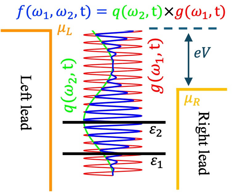
Figure 1: Schematic setup for quantum transport through a multi-level mesoscopic system driven simultaneously by two periodic oscillations.

II.4 Wangsness-Bloch-Redfield (WBR) QME

Here, our theoretical formulation of an open quantum system also starts with the Liouville-von Neumann (LvN) equation, i.e., Eq. (1). It is then followed by defining a rotation protocol (known as the interaction picture) for the operator $\hat{O}$ as

$$\tilde{O}(t)=U_{B}^{\dagger}(t,t_{0})U_{S}^{\dagger}(t,t_{0})\,\hat{O}(t)\,U_{S}(t,t_{0})\,U_{B}(t,t_{0}),$$ (30)

which is basically a rotation protocol in terms of the time evolution operators of the system and bath Hamiltonians, which are defined as:

$$U_{S}(t,t_{0})\!=\!\mathcal{T}e^{-i\int_{t_{0}}^{t}\hat{H}_{S}(s)\,ds},\,U_{B}(t,t_{0})\!=\!e^{-i\hat{H}_{B}(t-t_{0})}.~~~~~$$ (31)

It should be highlighted that we have used the general time-evolution operator (with the time-ordering operator $\mathcal{T}$) for the system part because the system Hamiltonian, $H_{S}(t)$, is time-dependent in our problem. We also stress that $H_{S}(t)$ will carry the dependency on $t_{0}$, even though we have kept only $t$ for the sake of simplicity. Applying the above transformation to the Hamiltonian and density operator leads to the following transformed Liouville-von Neumann (LvN) equation:

$$\frac{d\tilde{\rho}(t)}{dt}=-{i}[\tilde{H}_{SB}(t),\tilde{\rho}(t)].$$ (32)

We proceed by taking the time integral of the above LvN equation and substituting the integral expression back into the same relation (to make the equation more self-contained) as:

$$\begin{aligned} \frac{d\tilde{\rho}(t)}{dt}=&-i[\tilde{H}_{SB}(t),\tilde{\rho}(t_{0})]\\ &-\int_{t_{0}}^{t}[\tilde{H}_{SB}(t),[\tilde{H}_{SB}(t^{\prime}),\tilde{\rho}(t^{\prime})]]\,dt^{\prime}.\end{aligned}$$ (33)

At this point, we invoke three famous approximations [35]: 1) factorization of initial states which says that the density operators of the system and the bath are uncorrelated at $t_{0}$ such that $\tilde{\rho}(t_{0})\!=\!\tilde{\rho}_{S}(t_{0})\otimes\tilde{\rho}_{B}$. 2) Born approximation, which says that the density operators of the system and the bath are uncorrelated at other times so that the system density operator can be obtained by tracing over the bath $\tilde{\rho}_{S}(t)=\operatorname{Tr}_{B}(\tilde{\rho}_{S}(t)\otimes\tilde{\rho}_{B})$. 3) the Markov approximation which implies that the evolution of the system depends only on the present state and not on its history (i.e., the $d\tilde{\rho}(t)/dt$ on the left side of Eq. (33), has to be determined only by $\tilde{\rho}(t)$ at the same time on the right side of the equation). Note that the Markov approximation makes the dynamic time-local and it can be justified in the weak coupling regime. Changing the integration variable from $t^{\prime}$ to $\tau=t-t^{\prime}$ makes the upper limit of the integration to be $(t-t_{0})$. Markov approximation also tells us that, in the long-time limit, $t-t_{0}$ is large compared to the bath correlation time such that $(t-t_{0})$ can be replaced by $\infty$. After all approximations implemented, we arrive at the expression

$$\begin{aligned} \frac{d\tilde{\rho}_{S}(t)}{dt}\!=\!-\!\int_{0}^{\infty}\!&\operatorname{Tr}_{B}[\tilde{H}_{SB}(t),[\tilde{H}_{SB}(t-\tau),\tilde{\rho}_{S}(t)\\ &\otimes\tilde{\rho}_{B}]~]d\tau.\end{aligned}$$ (34)

Note that, the assumption of the bath being always at the thermal equilibrium is equivalent to defining the bath’s density operator as $\tilde{\rho}_{B}=exp(-\beta(\hat{H}_{B}-\mu\hat{n}_{B}))/Z_{B}$, where $\beta$, $\mu$, $\hat{n}_{B}$, and $Z_{B}$ are the inverse temperature energy, electrochemical potential, electronic number operator and the partition function of the bath respectively. With a thermal bath, one can show that $\operatorname{Tr}_{B}([\tilde{H}_{SB}(t),\tilde{\rho}(t_{0})])=0$. We then return Eq. (34) to the lab frame (schrödinger picture) by applying the system and bath unitary time evolutions in the reverse way of what was introduced in Eq. (30). A final compact relation can be given as:

$$\begin{aligned} \frac{d\hat{\rho}_{S}(t)}{dt}=-i[\hat{H}_{S}(t),&\hat{\rho}(t_{0})]-\int_{0}^{\infty}\operatorname{Tr}_{B}[\hat{H}_{SB},[\\ &\hat{\tilde{H}}_{SB}(\tau,t),\hat{\rho}_{S}(t)\otimes\hat{\rho}_{B}]]d\tau,\end{aligned}$$ (35)

with the following definition

$$\begin{aligned} &\hat{\tilde{H}}_{SB}(\tau,t)\!=\!\\ &U_{S}(t,t_{0})U_{B}(t,t_{0})\tilde{H}_{SB}(t\!-\!\tau)U_{B}^{\dagger}(t,t_{0})U_{S}^{\dagger}(t,t_{0})=~~~~\\ &U_{B}(\tau)U_{S}(t,t\!-\!\tau)\hat{H}_{SB}U_{S}^{\dagger}(t,t\!-\!\tau)U_{B}^{\dagger}(\tau),\end{aligned}$$ (36)

which, in turn, requires the following definitions

$$\begin{aligned} &U_{B}(\tau)=e^{-i\hat{H}_{B}\tau},~~U_{S}(t,t\!-\!\tau)=\mathcal{T}e^{-i\int_{t-\tau}^{t}\hat{H}_{S}(s)ds}.\end{aligned}$$ (37)

Notably, all exponential terms with $t_{0}$ have canceled each other due to their opposite signs. In addition, if we take $H_{S}$ time-independnet, WBR QME reduces to a well accepted form in which the evolution of $\hat{\tilde{H}}_{SB}$ only determines with the time difference $\tau$ [36]. Within the accepted approximations, Eq. (35) is very general and not limited to a specific form of time dependency for the system’s Hamiltonian. Eq. (35) requires significant simplifications before it can be used practically. Following cases in which system’s Hamiltonian is time-independent, we are expecting to arrive at explicit forms for dissipative terms, so-called dissipators. The final expression in Eq. (LABEL:eq:36) reflects a important observation: the possible dissipators would become time-dependent because $\hat{\tilde{H}}_{SB}$ itself is time-dependent. The process of deriving practical forms for the dissipators can be divided into three stages, as will be detailed in the following three subsections. In the first stage, we trace out the bath degrees of freedom. In the second stage, we perform the time integration over $\tau$. Finally, in the third stage, we apply the wide-band approximation to justify the final form of the dissipators.

II.5 Time-dependent dissipators for QME - I: tracing out bath

Here, we start by disentangling the double commutation and then substitute more explicit forms of $\hat{H}_{SB}$ and $\hat{\tilde{H}}_{SB}(\tau,t)$ in Eq. (35). To do this compactly, we first define the following expression

$$\hat{\tilde{H}}_{SB}(\tau,t)=\sum_{li}\tilde{C}_{\alpha i}^{\dagger}(\tau)\tilde{d}_{i}(t,\tau)+\tilde{d}_{i}^{\dagger}(t,\tau)\tilde{C}_{\alpha i}(\tau),~~~~~~$$ (38)

with the following definitions for explicit terms

$$\begin{aligned} \tilde{C}_{\alpha i}(\tau)&=U_{B}(\tau)\,\hat{C}_{\alpha i}\,U_{B}^{\dagger}(\tau)=\sum_{\alpha k}V_{\alpha k,i}^{\ast}\hat{c}_{\alpha k}e^{i\,\epsilon_{\alpha k}\tau}\\ \tilde{d}_{i}^{\,(\dagger)}(t,\tau)&=U_{S}(t,t\!-\!\tau)\,\hat{d}_{i}^{\,(\dagger)}\,U_{S}^{\dagger}(t,t\!-\!\tau).\end{aligned}$$ (39)

Exponential dependence of $\tilde{C}_{\alpha i}(\tau)$ to $\tau$ can be derived by using fermionic Pauli principle among bath’s operators and Baker-Campbell-Hausdorff formula, see Appendix A. Note that $\tilde{C}^{\dagger}_{\alpha i}(\tau)=\tilde{C}_{\alpha i}(\tau)^{\,\dagger}$ and $\tilde{d}^{\dagger}_{i}(t,\tau)=\tilde{d}_{i}(t,\tau)^{\,\dagger}$. Disentangling the double commutation yields four generic integrands. The first and second generic integrands read as $\hat{H}_{SB}\hat{\tilde{H}}_{SB}(\tau,t)\hat{\rho}_{S}(t)\otimes\hat{\rho}_{B}$, and $\hat{H}_{SB}\hat{\rho}_{S}(t)\!\otimes\!\hat{\rho}_{B}\hat{\tilde{H}}_{SB}(\tau,t)$. Each of these four generic integrands comprises four specific integrands. However, we only retain two of these specific integrands, in particular those in which similar operators multiply to their conjugate transpose. When faced with the first generic integrand, we only keep following two specific terms

$$\begin{aligned} \sum_{\smash{\alpha i,\beta j}}\,&\hat{C}_{\alpha i}^{\dagger}\hat{d}_{i}\tilde{d}_{j}^{\dagger}(t,\tau)\tilde{C}_{\beta j}(\tau)\hat{\rho}_{S}(t)\otimes\hat{\rho}_{B}+\\[-6.0pt] &\hat{d}_{i}^{\dagger}\hat{C}_{\alpha i}\tilde{C}_{\beta j}^{\dagger}(\tau)\tilde{d}_{j}(t,\tau)\hat{\rho}_{S}(t)\otimes\hat{\rho}_{B},\end{aligned}$$ (40)

which can be further rearranged as

$$\begin{aligned} \sum_{\smash{\alpha i,\beta j}}\,&\hat{C}_{\alpha i}^{\dagger}\tilde{C}_{\beta j}(\tau)\hat{\rho}_{B}\otimes\hat{d}_{i}\tilde{d}_{j}^{\dagger}(t,\tau)\hat{\rho}_{S}(t)+\\[-6.0pt] &\hat{C}_{\alpha i}\tilde{C}_{\beta j}^{\dagger}(\tau)\hat{\rho}_{B}\otimes\hat{d}_{i}^{\dagger}\tilde{d}_{j}(t,\tau)\hat{\rho}_{S}(t).\end{aligned}$$ (41)

We refer to the above two terms as the final first and second terms. Similarly, the final third and fourth non-vanishing integrands are

$$\begin{aligned} \sum_{\smash{\alpha i,\beta j}}\,&\hat{C}_{\alpha i}^{\dagger}\hat{\rho}_{B}\tilde{C}_{\beta j}(\tau)\otimes\hat{d}_{i}\hat{\rho}_{S}(t)\tilde{d}_{j}^{\dagger}(t,\tau)+\\[-6.0pt] &\hat{C}_{\alpha i}\hat{\rho}_{B}\tilde{C}_{\beta j}^{\dagger}(\tau)\otimes\hat{d}_{i}^{\dagger}\hat{\rho}_{S}(t)\tilde{d}_{j}(t,\tau).\end{aligned}$$ (42)

Now, we are ready to focus on the process of tracing out the bath degrees of freedom. Fundamentally, the thermal bath obeys the relations: $\operatorname{Tr}_{B}(\hat{c}_{\alpha k}^{\dagger}\hat{c}_{\beta k^{\prime}}\hat{\rho}_{B}(\mu))\!=\!f(\epsilon_{\alpha k},\mu_{\alpha})\delta_{k,k^{\prime}}\delta_{\alpha,\beta}$, and $\operatorname{Tr}_{B}(\hat{c}_{\alpha k}\hat{c}_{\beta k^{\prime}}^{\dagger}\hat{\rho}_{B}(\mu))\!=\!1\!-\!f(\epsilon_{\alpha k},\mu_{\alpha})\delta_{k,k^{\prime}}\delta_{\alpha,\beta}$ [37].

In dealing with the first term in Eq. (41), we should recall the explicit form of the operator $\hat{C}_{\alpha i}^{\dagger}$ from Eq. (29) and $\tilde{C}_{\alpha i}(\tau)$ from the first line of Eq. (39). Then, the double summation of the indices $k$ and $k^{\prime}$ reduces to only one summation, namely $k$. The same reduction in the summation index also applies to indices $\alpha$ and $\beta$. The process of tracing out the bath degrees of freedom in the second term of Eq. (41) is carried out using the same procedure. When tracing out the bath degrees of freedom, one has to be cautious with the third and fourth terms in Eq. (42), as the cyclic invariance of the trace must be utilized. Thereupon, tracing out the bath degrees of freedom gives us the following expression for the first four non-vanishing terms (out of eight)

$$\begin{aligned} &\int_{0}^{\infty}\!\!d\tau\!\!\sum_{\smash{\alpha k,ij}}\!V_{\alpha k,i}V_{\alpha k,j}^{\ast}f(\epsilon_{\alpha k},\mu_{\alpha})e^{i\,\epsilon_{\alpha k}\tau}\,\hat{d}_{i}\tilde{d}_{j}^{\dagger}(t,\tau)\hat{\rho}_{S}(t)+~~~~\\[-4.0pt] &V_{\alpha k,i}^{\ast}V_{\alpha k,j}(1\!-\!f(\epsilon_{\alpha k},\mu_{\alpha}))e^{-i\,\epsilon_{\alpha k}\tau}\,\hat{d}_{i}^{\dagger}\tilde{d}_{j}(t,\tau)\hat{\rho}_{S}(t)-~~~~\\ &V_{\alpha k,i}V_{\alpha k,j}^{\ast}(1\!-\!f(\epsilon_{\alpha k},\mu_{\alpha}))e^{i\,\epsilon_{\alpha k}\tau}\,\hat{d}_{i}\hat{\rho}_{S}(t)\tilde{d}_{j}^{\dagger}(t,\tau)-~~\quad\\ &V_{\alpha k,i}^{\ast}V_{\alpha k,j}f(\epsilon_{\alpha k},\mu_{\alpha})e^{-i\,\epsilon_{\alpha k}\tau~~}\,\hat{d}_{i}^{\dagger}\hat{\rho}_{S}(t)\tilde{d}_{j}(t,\tau).\end{aligned}$$ (43)

For the sake of clarity and brevity, we retain only the first four integrands of the full set of eight integrands, as it provides a sufficient description for the process of simplification of dissipators. Here, we highlight that performing the integration (analytically) is not feasible until the explicit dependence of $\tilde{d}_{i/j}$ and $\tilde{d}_{i/j}^{\dagger}$ to the $\tau$ is known.

II.6 Time-dependenet dissipators for QME - II: Intergation over $\tau$

A clear distinction between the time variables $t$ and $\tau$ is essential to enable integration over $\tau$. Thus, we must pay attention to the explicit dependence of $H_{S}$ on $t$ and $\tau$. In practice, we first need to identify the explicit form of $U_{S}(t,t\!-\!\tau)$, and then define $\tilde{d}_{j}(t,\tau)$ and $\tilde{d}^{\dagger}_{j}(t,\tau)$ as functions of $t$ and $\tau$. In general, when the Hamiltonian of the system is time-dependent, deriving an analytical form for the time-evolution operator is not a trivial task, primarily because $H_{S}(t)$ does not necessarily commute with itself at different times. This is also a central problem in the dynamical control of closed quantum systems (e.g., the Rabi model) [38]. Floquet theory provides an explicit form for the time-evolution operator when the Hamiltonian is exactly periodic, which is known as Shirley’s time-evolution formula [39]. In our previous work, we have shown that this form is advantageous for deriving a time-dependent dissipator. As demonstrated earlier, Floquet theory can be extended to multi-mode Floquet theory.

Now, we focus on the simplification of the dissipators by using the Floquet time evolution operator, Eq. (25), for $U_{S}^{\dagger}(t,t\!-\!\tau)$ as

$$\begin{aligned} U_{S}(t,t\!-\!\tau)=\sum_{mn}\langle mn|\hat{Y}e^{-i\hat{\Lambda}_{S}^{F}\tau}\hat{Y}^{\dagger}|00\rangle\,e^{in\omega_{1}t}e^{im\omega_{2}t},~~~~~\end{aligned}$$ (44)

in which $\Lambda_{S}^{F}$ is the diagonalized two-mode Floquet Hamiltonian as $\hat{\Lambda}_{S}^{F}=\hat{Y}^{\dagger}\hat{H}_{S}^{F}\hat{Y}$. In the above expression, the comma between the indices in the double-index bra-ket is omitted for simplicity. Note that the diagonalization operator is a unitary transformation operator, i.e., $\hat{Y}^{\dagger}\hat{Y}=\hat{1}$. Consequently, we can reexpress $\tilde{d}_{j}(t,\tau)$ and $\tilde{d}_{j}^{\,(\dagger)}(t,\tau)$, using Eq. (39) as

$$\begin{aligned} \tilde{d}_{i}^{\,(\dagger)}(t,\tau)=\sum_{mn,kq}\,&\langle mn|\hat{Y}e^{-i\hat{\Lambda}_{S}^{F}\tau}\hat{\mathcal{D}}_{i}^{o\,(\dagger)}e^{i\hat{\Lambda}_{S}^{F}\tau}\hat{Y}^{\dagger}|kq\rangle\times\\ \,&e^{i(n-q)\omega_{1}t}e^{i(m-k)\omega_{2}t},\end{aligned}$$ (45)

in which we have defined $\hat{\mathcal{D}}_{i}^{o}\!\!=\!\!\hat{Y}^{\dagger}|00\rangle\hat{d}_{i}\langle 00|\hat{Y}$. $\tilde{d}^{\dagger}_{j}(t,\tau)$ defines in the same manner by replacing $\hat{\mathcal{D}}_{i}^{o}$ with $\hat{\mathcal{D}}_{i}^{o\dagger}\!=\!\hat{Y}^{\dagger}|00\rangle\hat{d}_{i}^{\dagger}\langle 00|\hat{Y}$. Now, the distinction between $\tau$ and $t$ becomes evident in Eq. (45). At this stage, it is necessary to choose the basis set for the Hilbert space, $\{|a\rangle\}$, so that operators can be expressed as matrices. For instance, the elements of the density operator can be written as $\rho_{ab}(t)\!=\!\langle a|\hat{\rho}(t)|b\rangle$. By reducing operators to matrices, particularly the rotating matrix $Y$, we can work within the diagonalized two-mode Floquet space, $\{|\gamma\rangle\}$, such that $\langle\gamma|\hat{\Lambda}_{S}^{F}\!=\!\langle\gamma|\mathcal{E}_{\gamma}$. This allows us to express the matrix elements of the central operator within the bracket in Eq. (45) as

$$\begin{aligned} \left(e^{-i\hat{\Lambda}^{F}\tau}\hat{D}_{j}^{o(\dagger)}e^{i\hat{\Lambda}^{F}\tau}\right)_{\gamma\nu}=e^{-i\Omega_{\gamma\nu}\tau}\left(\hat{D}_{j}^{o(\dagger)}\right)_{\gamma\nu},\end{aligned}$$ (46)

where $\Omega_{\gamma\nu}\!=\!\mathcal{E}_{\gamma}\!-\!\mathcal{E}_{\nu}$. Note that, we combined the two oppositely signed exponential terms into a single expression. Now, we are in the position to perform integration over $\tau$ as

$$\begin{aligned} \int_{0}^{\infty}\!\!\!\!e^{\pm i(\epsilon_{\alpha k}\mp\Omega_{\gamma\nu})\tau}\!d\tau\!=\!\pi\delta(\epsilon_{\alpha k}\!\mp\!\Omega_{\gamma\nu})\!\pm\!i\mathcal{P}(\!\frac{1}{\epsilon_{\alpha k}\!\mp\!\Omega_{\gamma\nu}}\!),~~~~\end{aligned}$$ (47)

in terms of the delta function and the Cauchy’s principal value, see Appendix B. Hereafter, we neglect the Cauchy’s principle term.

II.7 Time-Dependenet dissipators for QME - III: final step

At this point, before substituting $\tilde{d}^{\dagger}$ and $\tilde{d}$ into Eq. (LABEL:eq:43), we shall invoke the wide-band approximation. In general, when the electronic levels in the bath are very closely spaced we can replace the summation, over $k$, by an integral as

$$\begin{aligned} \sum_{\alpha k}\rightarrow\sum_{\alpha}\int D^{\alpha}(\epsilon_{\alpha k})d\epsilon_{\alpha k}\end{aligned}$$ (48)

In the wide-band approximation, it is assumed that the DOS of an ideal bath, $D^{\alpha}$, does not change significantly over the range of energies relevant to the transport such that

$$\begin{aligned} \Gamma_{ij}^{\alpha}=2\pi V_{\alpha k,i}V_{\alpha k,j}^{*}D^{\alpha}\approx\text{constant}.\end{aligned}$$ (49)

$\Gamma_{ij}^{\alpha}$ is the coupling rate of the bath $\alpha$. We can perform the integration over $\epsilon_{\alpha k}$ in which the Fermi function essentially picks out the element $\Omega_{\gamma\nu}$. With that, the first four lead-specific dissipators (relevant to the bath $\alpha$) can be simplified as

$$\begin{aligned} \mathfrak{D}_{\alpha}^{I-IV}\!=\!\sum_{\smash{ij}}&\frac{\Gamma_{ij}^{\alpha}}{2}{d}_{i}\mathbb{d}_{\alpha,j}^{\dagger\,+}(t){\rho}_{S}(t)+\frac{\Gamma_{ji}^{\alpha}}{2}{d}_{i}^{\,\dagger}\mathbf{\bar{\text{$\mathbb{d}$}}}_{\alpha,j}^{\,\,\,-}(t){\rho}_{S}(t)~~~~~\\ -&\frac{\Gamma_{ij}^{\alpha}}{2}{d}_{i}{\rho}_{S}(t)\mathbf{\bar{\text{$\mathbb{d}$}}}_{\alpha,j}^{\dagger\,+}(t)-\frac{\Gamma_{ji}^{\alpha}}{2}{d}_{i}^{\,\dagger}{\rho}_{S}(t)\mathbb{d}_{\alpha,j}^{\,\,\,-}(t),\end{aligned}$$ (50)

where we have defined new time-dependent matrices

$$\begin{aligned} \mathbb{d}_{\alpha,j}^{(\dagger)\,\pm}(t)\!=\!\!\sum_{mn,kq}&\!\!\langle mn|Yf(\pm\Omega,\mu_{\alpha})\circ\mathcal{D}_{j}^{o\,(\dagger)}Y^{\dagger}|kq\rangle\times\\ &e^{i(n-q)\omega_{1}t}e^{i(m-k)\omega_{2}t},\\ \mathbf{\bar{\text{$\mathbb{d}$}}}_{\alpha,j}^{(\dagger)\,\mp}(t)\!=\!\!\sum_{mn,kq}\!\!&\langle mn|Y(1\!-\!f(\mp\Omega,\mu_{\alpha}))\circ\mathcal{D}_{j}^{o\,(\dagger)}Y^{\dagger}|kq\rangle\times\quad\\ \,&e^{i(n-q)\omega_{1}t}e^{i(m-k)\omega_{2}t}.\end{aligned}$$ (51)

Note that in Eq. (51), there are two types of occupation matrices: electron occupation, $f(\pm\Omega,\mu_{\alpha})$, and hole occupation, $1-f(\mp\Omega,\mu_{\alpha})$. These occupation matrices multiply to $\mathcal{D}_{j}^{o(\dagger)}$ by the Hadamard product, remarked by $\circ$. Accordingly, one can follow the same procedure for the second four non-vanishing dissipators, $\mathfrak{D}_{\alpha}^{V-VIII}({\rho}_{S}(t),t)$. However, the second set of four non-vanishing dissipators is the Hermitian conjugates of the first set. This symmetry can be utilized to reduce the computational cost of calculations. Finally, we can have the following compact dynamical equation for the reduced density matrix, $\rho_{S}(t)$, as

$$\begin{aligned} \frac{d\rho_{S}(t)}{dt}=-i[H_{S}(t),\rho_{S}(t)]-\sum_{\alpha}\mathfrak{D}_{\alpha}^{I-VIII}({\rho}_{S}(t),t).~~~~\end{aligned}$$ (52)

Extending the spinless quantum transport theory to the spinful counterpart is a straightforward process. First, annihilation (creation) operators must receive the spin degrees of freedom, $\sigma\in\{\uparrow,\downarrow\}$, as $\hat{d}_{i,\sigma}$ ($\hat{d}_{i,\sigma}^{\,\dagger}$). Consequently, we should define $\hat{\mathcal{D}}_{i,\sigma}^{o}\!=\!\hat{Y}^{\dagger}|00\rangle\hat{d}_{i,\sigma}\langle 00|\hat{Y}$ and so on. This essentially indicates that all matrix operators in Eq. (50) and Eq. (51) should be decorated with the spin degrees of freedom such that one should consider both the spin-up and spin-down dissipators.

II.8 Observables

Essentially, we need to define the system’s electronic number operator in the Hilbert space as $\hat{n}_{S}=\sum_{i}\hat{d}_{i}^{\dagger}\hat{d}_{i}$. With that, we can evaluate the expectation of the system’s particle number, $\langle\hat{n}_{S}\rangle(t)$ (known also as the total occupation or the charge number). Similarly, the electron number operator for each lead is defined as $\hat{n}_{\alpha}\!=\!\sum_{k}\hat{c}_{\alpha k}^{\dagger}\hat{c}_{\alpha k}$, where $\alpha\in\{L,R\}$. The total charge number of the system at time t is given by

$$\begin{aligned} \langle\hat{n}_{S}\rangle(t)=\operatorname{Tr}(\hat{n}_{S}\hat{\rho}_{S}(t)).\end{aligned}$$ (53)

The second observable is the terminal current. In general, the particle current operator passing through the terminal $\alpha$, $\hat{I}_{\alpha}$, is defined as the rate of change of the total particle number in that lead as: ${d\langle\hat{n}_{\alpha}\rangle(t)}/{dt}={d(\hat{n}_{\alpha}\hat{\rho}(t))}/{dt}$. Based on particle conservation, one can perceive that the rate of particle change in the reduced system is the sum of the currents passing through all terminals. Hence, one can reversely define the current operator as

$$\begin{aligned} \frac{d\langle\hat{n}_{S}\rangle(t)}{dt}&=\operatorname{Tr}\big{(}\hat{n}_{S}\frac{d\hat{\rho}_{S}(t)}{dt}\big{)}\\ &=\!\sum_{\alpha}\operatorname{Tr}\big{(}\hat{n}_{S}\,\hat{\mathfrak{D}}_{\alpha}^{I-VIII}(\hat{\rho}_{S}(t),t)\big{)}\!=\!\sum_{\alpha}\hat{I}_{\alpha}(t).~~~~\end{aligned}$$ (54)

Note that, in the above expression, we make use of Eq. (52) and $\operatorname{Tr}(\hat{n}_{S}[\hat{H}_{S}(t),\hat{\rho}_{S}(t)])\!=\!0$ due to the cyclic invariance of the trace and the fact that for fermions $[\hat{H}_{S},\hat{n}_{S}]=0$. In addition, $[\hat{H}_{S}(t),\hat{\rho}_{S}(t)]$ describes the evolution of the density operator that merely originated from the system’s Hamiltonian (the closed system) and this part of evolution does not change the expectation value of $\hat{n}_{S}$.

Here, with regard to the static aspect of transport, we cannot properly define the concept of a steady-state observable in the long-time limit for scenarios involving two periodic drivings, as the off-diagonal coupling is not necessarily perfectly periodic. This means that the system observable in the long-time limit may not settle to a steady constant value, instead it may oscillate unpredictably. Nonetheless, one can have the following definition for a quasi-steady state observable,

$${O}^{q}=\lim_{t\to\infty}\frac{1}{\mathscr{T}}\int_{0}^{\mathscr{T}}dt\,{O}(t),$$ (55)

where $\mathscr{T}$ indicates the period by which the observable oscillates. For observables in a spinful study, one should employ the spin-resolved number operators $\hat{n}^{\sigma}_{S}=\sum_{i}\hat{d}_{i,\sigma}^{\dagger}\hat{d}_{i,\sigma}$ in Eqs. (53) and (54) to distinguish between spin-up and spin-down observables.

III Representative Applications

III.1 Transport through a spinless two-level dot

As preliminary applications of Eqs. (50)-(55), let us to consider transport through a spinless two-level dot driven by a primary off-diagonal coupling, $g(\omega_{1},t)$, oscillating at $\omega_{1}$ and a secondary off-diagonal or diagonal coupling, $q(\omega_{2},t)$, oscillating at $\omega_{2}$. The general one-body Hamiltonian matrix of such a two-level system can be expressed as

$$h(\omega_{1},\omega_{2},t)\!=\!\!\begin{bmatrix}\epsilon_{1}&\!g(\omega_{1},t)\!\odot\!q(\omega_{2},t)\\ g^{*}(\omega_{1},t)\!\odot\!q^{*}(\omega_{2},t)&\!\epsilon_{2}\vee\epsilon_{2}+q(\omega_{2},t)\end{bmatrix},~~~~~$$ (56)

where $\odot\!\in\!\{+,\times\}$, and $\vee$ indicates the OR operator. Here, the goal is to inspect how incorporating a secondary driving term within different scenarios will alter the transport characteristics. Both the time-dependent and quasi-steady-state characteristics will be investigated. We recall that the current-voltage characteristic of a non-driven non-interacting multi-level system shows the typical steplike increase (conductance step) as the bias voltage increases, where each step corresponds to involving a new level into the transport. Here, voltage refers to $\mu_{L}\!-\!\mu_{R}$. In our previous work, we observed that a cosine off-diagonal coupling (corresponding to $g(\omega_{1},t)\!=\!A_{1}\cos(\omega_{1}t)$ and $q(\omega_{2},t)\!=\!0$) gives rise to the doubling of the conductance steps when the coupling strength, $A_{1}$, is large compared to the energy difference between the two levels, $\Delta\epsilon\!=\!\epsilon_{2}\!-\!\epsilon_{1}$. It is observed that the largest changes in conductance steps occur in the strong coupling regime when the driving frequency resonates with the energy difference between the two levels, $\omega_{1}\!=\!\Delta\epsilon$, and $A_{1}\!=\!\Delta\epsilon/2$; see the cane-colored line in Figs. 2 (a) and (b). Here, in the first few examples, we keep the simulation temperature at $4.2K^{o}$ (equivalent to the temperature energy $1/\beta\!\approx\!0.36\,meV$) because in the low-temperature regime, the thermal energy does not cause significant smearing of the Fermi distribution, leading to sharp conductance steps and hence driven induced effects can be more pronounced. Following our previous work, energy-related parameters are given in $eV$, and hereafter the unit is omitted for simplicity. We set $\epsilon_{1}\!=\!-0.1$, $\epsilon_{2}\!=\!+0.1$, and the left and right electrodes are parameterized by the coupling rate of $\Gamma_{ji}^{L/R}\!=\!0.005$. Hereafter, $\mu_{R}$ (drain) is fixed at a negative minimum voltage, $V_{min}$, far below $\epsilon_{1}$, while $\mu_{L}$ sweeps within the range [$V_{min}$,$V_{max}$].

1. Driven by adding a secondary (off-resonance) off-diagonal term to the main (in-resonance) off-diagonal driving: In the first set of examples, we define $h_{22}(t)\!=\!\epsilon_{2}$, $\odot\!=\!+$, $q(\omega_{2},t)\!=\!A_{2}\sin(\omega_{2}t)$ (the secondary oscillatory term), and $g(\omega_{1},t)\!=\!A_{1}\sin(\omega_{1}t)$ (the primary off-diagonal coupling). The main frequency is fixed at $\omega_{1}\!=\!0.2$ (in resonance), and the driving amplitudes are set equal with $A_{1}\!=\!A_{2}\!=\!0.05$. In Figs. (2) (a) and (b), we present the system’s quasistatic particle number and the left terminal’s quasistatic current for two values of the secondary frequency: $\omega_{2}\!=\!0.150$, and $\omega_{2}\!=\!0.175$ (off resonance).

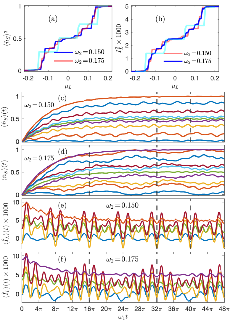
Figure 2: quasistatic and dynamics of an open two-level dot driven by two additive drivings. (a) quasistatic charge number and (b) quasistatic current at the left terminal. (c)-(f) the corresponding time-dependent charge number and current at the left terminal.

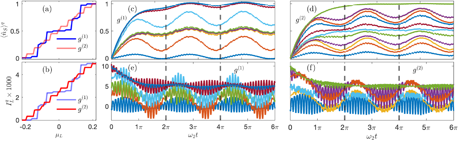
Figure 3: Quasistatic and dynamics of an open two-level dot driven by multiplying an envelope function to the main in-resonance off-diagonal driving. (a) quasistatic charge number and (b) quasistatic current at the left terminal for real and complex valued primary drivings as $g^{(1)}\!=\!A_{1}\sin(\omega_{1}t)$, and $g^{(2)}\!=\!A_{1}(\cos(\omega_{1}t)\!+\!i\sin(\omega_{1}t))$. (c) and (d) are the time-dependent charge number corresponding to the plateaus in (a). (e) and (f) time-dependent current at the left terminal corresponding to the few main plateaus in (b). Curves with the same color in (c) and (e) are associated with each other and same for (d) and (f).

One can observe how secondary driving significantly influenced the number of quantized steps. In Figs. (2) (a) and (b), we also show the results of the single mode Floquet QME using solid cane-colored lines for comparison. This is done by setting $A_{1}\!=\!0.1$ and $A_{2}\!=\!0$ and can be considered as one of the simplest validity checks for the presented two-mode Floquet QME as it reproduces results from previous work [28]. In Figs. 2 (c) and (d), we plot the time-dependent charge number for the two frequencies, corresponding to selected steps from Fig. 2(a). Similarly, in Figs. 2 (e) and (f), we plot the time-dependent current at the left terminal for the two frequencies, corresponding to selected steps from Fig. 2(b). Here, we highlight that the oscillatory behavior of $\langle\hat{n}_{S}\rangle(t)$ requires setting $\mathscr{T}\!=\!4T_{1}$ and $\mathscr{T}\!=\!8T_{1}$ for $\omega_{2}\!=\!0.150$ and $\omega_{2}\!=\!0.175$, respectively. The vertical dashed lines show the time intervals $4T_{1}$ and $8T_{1}$ [$8T_{1}$ and $16T_{1}$] in Figs. (2) (c) and (e) [Figs. (2) (d) and (f)]. Here, the integer ratios between the two frequencies are $4/3$ and $8/7$ which indicates the period by which the observables oscillate determines by the in-resonance frequency. Compared to the single-frequency case (cane-colored lines), two key differences in the results can be reported. First, the number of conductance steps increased noticeably, such that for the case of $\omega_{2}\!=\!0.150$ there are six large steps and four small steps. For the case of $\omega_{2}\!=\!0.175$, there are 14 steps in total. Secondly, observables are no longer static variables but rather quasistatic.

2. Driven by multiplying a far off-resonance term to the main in-resonance off-diagonal driving: In the second set of examples, we set $h_{22}(t)\!=\!\epsilon_{2}$, $\odot\!=\!\times$, and $q(\omega_{2},t)\!=\!A_{2}\sin^{2}(\omega_{2}t)$. We then take two forms for $g(\omega_{1},t)$ as: (I) the real-valued $g^{(1)}\!=\!A_{1}\sin(\omega_{1}t)$ and (II) the complex-valued $g^{(2)}\!=\!A_{1}(\cos(\omega_{1}t)\!+\!i\sin(\omega_{1}t))$. The main and second frequencies are fixed at $\omega_{1}\!=\!0.2$ (in resonance) and $\omega_{2}\!=\!0.02$ (ten times smaller, far off resonance). The driving amplitudes are set to $A_{1}\!=\!0.1$, and $A_{2}\!=\!1.0$, ensuring that $q(\omega_{2},t)$ acts as an envelope function. The maximum total amplitude, $A_{1}A_{2}$, remains consistent with the previous set of examples, corresponding to the strong interacting regime. In Figs. (3) (a) and (b), we present the two main quasistatic observables for the real and complex-valued forms of the primary driving function, $g$. Clearly, the complex-valued driving increased the number of plateaus in an intricate way. In Figs. (3) (c) and (d) [(e) and (f)], we have plotted the time-dependent charge number [left terminal current] associated with $g^{(1)}$ and $g^{(1)}$ for a few selected steps. Here, the oscillation behavior of the dynamical observables requires to set $\mathscr{T}\!=\!T_{2}$ as we indicated the sampling time by the last vertical dashed-lines in Figs. (3) (c)-(f). These dynamical results are interesting, particularly Figs. (3) (c) and (d), because it shows how the rise and fall of the slow envelope function influence the semi-steady behavior of the time-dependent charge number. We remind the reader that the time-dependent charge number shows an almost steady behavior when the dot is driven only by an off-diagonal single-frequency term [28].

3. Driven simultaneously by a secondary diagonal and a primary off-diagonal driving terms: In the third set of examples, we set $h_{12}(t)\!=\!h_{21}(t)\!=\!g(\omega_{1},t)\!=\!A_{1}\sin(\omega_{1}t)$, and $h_{22}(t)\!=\!\epsilon_{2}\!+\!A_{2}\cos(\omega_{2}t)$ such that the two-level system is driven simultaneously by both a primary off-diagonal and a secondary diagonal terms. The frequency and amplitude of the primary driving are fixed at $\omega_{1}\!=\!0.2$ and $A_{1}\!=\!0.1$, and we sweep over the few values for $\omega_{2}$ and $A_{2}$ to investigate who tuning the variables associated with secondary diagonal driving will alter the dynamic and quasistatic pattern of the two main observables. In Figs. 4 (a) and (b), we present the left terminal quasistatic current while fixing $\omega_{2}\!=\!0.10$ and $A_{2}\!=\!0.10$, respectively. Clearly from Fig. (4) (a), adding a secondary on-diagonal oscillatory driving emerges as doubling the four major current plateaus of the single-frequency driven two-level system. As the second intensity increases, the width of the emergent plateau also increases. The height of these emergent plateaus can be adjusted by altering the second frequency, as depicted in the Fig. (4) (b). In addition, changing the second frequency also modifies the onset of the emergent plateaus. Here, we must highlight that the quasistatic charge number associated with Figs. 4 (a) and (b), not presented here, follows an identical step-like pattern shown in the same figures, except that its maximum reaches a value of 1.0. In Figs. (4) (c) and (d), we plot the time-dependent left terminal current and the corresponding time-dependent charge number associated with several plateaus using the inputs: $A_{1}\!=\!0.1$, $\omega_{1}\!=\!0.2$, $A_{2}\!=\!0.08$, and $\omega_{2}\!=\!0.08$. As the electrochemical potential increases, the waveform of the time-dependent current also changes.

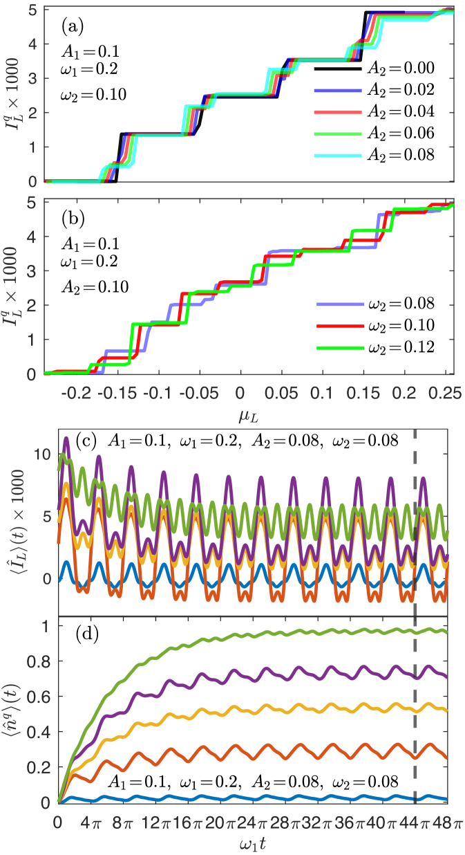
Figure 4: Transport trough a spinless two-level dot driven simultaneously by a primary (in-resonance) off-diagonal driving as $h_{12}(t)\!=\!A_{1}\sin(\omega_{1}t)$ and a secondary diagonal term as $h_{22}(t)\!=\!\epsilon_{2}\!+\!A_{2}\cos(\omega_{2}t)$. (a) quasistatic current at the left terminal while sweeping over the amplitude of the secondary driving. (b) same as (a) but sweeping over three frequencies of the secondary driving. (c) and (d) are time-dependent current at the left terminal and the time-dependent charge number corresponding to a few values of $\mu_{L}$ on the second curves in (b). Curves with the same color in (c) and (d) are associated with each.

Here, in this driving scenario, the integer ratios between the two frequencies can be used to determine the period over which the observables oscillate. For example in Fig. (4) (b), the integer ratios between the two frequencies are $5/1$, $2/1$, and $5/3$ for the three curves. These ratios indicate that one must employ $5T_{1}$ [$2T_{1}$] for $\omega_{2}\!=\!0.08$ or $\omega_{2}\!=\!0.12$ [$\omega_{2}\!=\!0.1$] when evaluating quasistatic expectation values. Interestingly, the time-dependent charge number shows triangle waveforms in the first emerged plateaus with a period of $2T_{1}$, see the second curve from bottom in Fig. (4) (d).

III.2 Transport through a spinful two-level dot

Here, we will add an electron-electron (e-e) interaction term as $\hat{H}^{ee}\!=\!\sum_{i}u_{i}\hat{d}_{i,\uparrow}^{\dagger}\hat{d}_{i,\uparrow}\hat{d}_{i,\downarrow}^{\dagger}\hat{d}_{i,\downarrow}$ to the system’s Hamiltonian in Eq. (27). The numerical calculation follows by considering spin-up and spin-down dissipators in the evolution of the density matrix and evaluating spin-resolved observables. Here, we have chosen this example based on the last spinless case as described below;

Driven simultaneously by the secondary diagonal and primary off-diagonal drivings in pretense of electron-electron interaction: In the fourth set of examples, we set $h_{11,\uparrow/\downarrow}\!=\!\epsilon_{1}$, $h_{12,\uparrow/\downarrow}(t)\!=\!h_{21,\uparrow/\downarrow}(t)\!=\!A_{1}\sin(\omega_{1}t)$, and $h_{22,\uparrow/\downarrow}(t)\!=\!\epsilon_{2}\!+\!A_{2}\cos(\omega_{2}t)$. The frequencies and amplitudes are fixed at $\omega_{1}\!=\!0.2$, $\omega_{2}\!=\!0.1$, and $A_{1}\!=\!A_{2}\!=\!0.1$, identical to the input variables used to obtain the red-colored curve in Fig. 4 (b). In Fig. 5 (a), we present the left terminal quasistatic current in the absence ($u_{1,2}\!=\!0$) and presence of the e-e interaction with the interaction strength $u_{1,2}\!=\!0.1$.

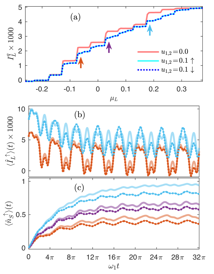
Figure 5: Transport trough a spinfull two-level dot driven simultaneously by primary (in-resonance) off-diagonal drivings as $h_{12,\uparrow/\downarrow}(t)\!=\!A_{1}\sin(\omega_{1}t)$ and secondary diagonal term as $h_{22,\uparrow/\downarrow}(t)\!=\!\epsilon_{2}\!+\!A_{2}\cos(\omega_{2}t)$. (a) the quasistatic current at the left terminal in the absence and presence of the e-e interaction is shown by a red and cane (blue dashed) lines, respectively. (b) the time-dependent current at the left terminal corresponding to the two values of $\mu_{L}$ in (a). Here, the solid (doted) line corresponds to the absence (presence) of the e-e interaction. (c) same as (b) for the time-dependent charge number. Curve’s color in (b) and (c) are associated with the color of vertical arrow’s in (a).

The main consequence of the e-e interaction in the quasistatic observables is to lower the height conductance steps. One can perceive that the interplay between the drivings and e-e interaction does not promote the spin polarization in the current. In Fig. 5 (b) [(c)], we plot the time-dependent current at the left terminal [time-dependent charge number] for two [three] values of $\mu_{L}$ in (a). Here, thicker solid (doted) lines correspond to plateaus calculated in the absence (presence) of the e-e interaction. From Fig. 5 (b), we can understand that the e-e interaction mainly lowers maximums of local peaks in an alternative way. In contrast, by looking at Fig. 5 (c), it can be understood that the e-e interaction lowers the height of the charge number in a uniform way.

IV Conclusion

In summary, we developed a general two-mode Floquet QME framework capable of accounting for a class of complex driving scenarios, where two oscillating terms jointly drive a multi-level open quantum system. In particular, we have explicitly derived the two-mode Floquet Liouville-von Neumann equation for the Floquet density operator which is exact. Next, we establish a connection between this equation and the two-mode Shirley’s-like time evolution operator in Hilbert space. This time evolution formula is a crucial tool that enables us to derive a series of time-local dissipators for a multi-level open quantum system that is driven simultaneously by two independent oscillating terms. Additionally, we have made a clear connection between the equation of motion and the time-averaged observables, and demonstrated the application of our two-mode Floquet QME through a number of quantum transport examples. Compared to our previous work, on spinless single-mode driven open quantum system, we have found that including a secondary oscillatory driving gives rise to increasing number of quantized plateaus in the current-voltage characteristics such that one can engineer the appearance of conductance steps by choosing appropriate driving frequencies, and amplitudes within different two-mode driving scenarios. In addition, we show that a certain two-mode complex-valued driving scenario results in a significant increase in quantized plateaus. Furthermore, we have comprehensively explored how different driving scenarios affect the dynamical behavior of observables. In a spinfull system, we show that including a moderate electron–electron term in the system’s Hamiltonian mainly results in lowering the hight of few quantized plateaus. We expected that the newly developed two-mode Floquet QME can be applicable in a large number of dissipative systems, as long as the system-bath coupling is not so strong since our two-mode Floquet QME is obtained by well-justified approximations. Although the present work is mainly focuses on the transport studies in finite temperature and arbitrary voltage, but we expect this work finds more applications in other areas such as quantum thermodynamics, Floquet engineering, quantum information, strongly correlated quantum systems.

Appendix A Explicit form of $\tilde{C}^{(\dagger)}_{\alpha i}(\tau)$

The initial step toward understanding how the bath’s correlation function relates to $\tau$ can be achieved by employing the Baker-Campbell-Hausdorff (BCH) expansion, $e^{\hat{A}}\hat{B}e^{-\hat{A}}\!=\!\hat{B}\!+\![\hat{A},\hat{B}]\!+\!{1}/{2!}\,[\hat{A},[\hat{A},\hat{B}]]\!+\!\dots$, as follows:

$$\begin{aligned} &\tilde{C}_{\alpha i}(\tau)=e^{-i\hat{H}_{B}\tau}\,\hat{C}_{\alpha i}\,e^{i\hat{H}_{B}\tau}=\hat{C}_{\alpha i}+\\ &(-i\tau)[\hat{H}_{B},\hat{C}_{\alpha i}]+\frac{(-i\tau)^{2}}{2!}[\hat{H}_{B},[\hat{H}_{B},\hat{C}_{\alpha i}]]+\dots,\\ \end{aligned}$$ (57)

which in turn requires evaluation of the commutation

$$\begin{aligned} &[\hat{H}_{B},\hat{C}_{\alpha i}]=[\sum_{\alpha^{\prime}k^{\prime}}\epsilon_{\alpha^{\prime}k^{\prime}}\hat{c}_{\alpha^{\prime}k^{\prime}}^{\dagger}\hat{c}_{\alpha^{\prime}k^{\prime}},\sum_{k}V^{\ast}_{\alpha k,i}\hat{c}_{\alpha k}]=\sum_{\alpha^{\prime}k^{\prime},k}\epsilon_{\alpha^{\prime}k^{\prime}}\\ &V^{\ast}_{\alpha k,i}[\hat{c}_{\alpha^{\prime}k^{\prime}}^{\dagger}\hat{c}_{\alpha^{\prime}k^{\prime}},\hat{c}_{\alpha k}]=\sum_{\alpha^{\prime}k^{\prime},k}(-\epsilon_{\alpha^{\prime}k^{\prime}})V^{\ast}_{\alpha k,i}\times\\ &\{\hat{c}_{\alpha^{\prime}k^{\prime}}^{\dagger},\hat{c}_{\alpha k}\}\hat{c}_{\alpha^{\prime}k^{\prime}}=\sum_{k}(-\epsilon_{\alpha k})V^{\ast}_{\alpha k,i}\hat{c}_{\alpha k}.\end{aligned}$$ (58)

Here, we have used $[AB,C]\!=\!A\{B,C\}\!-\!\{A,C\}B$ and $\{\hat{c}_{\alpha^{\prime}k^{\prime}}^{\dagger},\hat{c}_{\alpha k}\}\!=\!\delta_{\alpha^{\prime}\alpha}\delta_{k^{\prime}k}$. Consequently, $[\hat{H}_{B},[\hat{H}_{B},\hat{C}_{\alpha i}]]\!=\!\sum_{k}(-\epsilon_{\alpha k})^{2}V^{\ast}_{\alpha k,i}\hat{c}_{\alpha k}$. Substituting the results of commutations in the BCH formula gives

$$\begin{aligned} &\tilde{C}_{\alpha i}(\tau)=\sum_{k}V^{\ast}_{\alpha k,i}\hat{c}_{\alpha k}+\sum_{k}(i\epsilon_{\alpha k}\tau)V^{\ast}_{\alpha k,i}\hat{c}_{\alpha k}+\\ &\sum_{k}\frac{1}{2!}(i\epsilon_{\alpha k}\tau)^{2}V^{\ast}_{\alpha k,i}\hat{c}_{\alpha k}+\dots=\sum_{k}V^{\ast}_{\alpha k,i}\hat{c}_{\alpha k}e^{i\epsilon_{\alpha k}\tau}.\quad\end{aligned}$$ (59)

For the explicit form of $\tilde{C}^{\dagger}_{\alpha i}(\tau)$, we can simply employ $\tilde{C}^{\dagger}_{\alpha i}(\tau)=\tilde{C}_{\alpha i}(\tau)^{\,\dagger}$ as

$$\begin{aligned} &\tilde{C}_{\alpha i}^{\dagger}(\tau)=\sum_{k}V_{\alpha k,i}\hat{c}_{\alpha k}^{\dagger}e^{-i\epsilon_{\alpha k}\tau}.\end{aligned}$$ (60)

In addition, one can also proceed with the BCH expansion process, which leads to $[\hat{H}_{B},\hat{C}_{\alpha i}^{\dagger}]=\sum_{k}\epsilon_{\alpha k}V_{\alpha k,i}\hat{c}_{\alpha k}^{\dagger}$, and $[\hat{H}_{B},[\hat{H}_{B},\hat{C}_{\alpha i}^{\dagger}]]=\sum_{k}(\epsilon_{\alpha k})^{2}V_{\alpha k,i}\hat{c}_{\alpha k}^{\dagger}$. Nonetheless, the explicit form of $\tilde{C}^{\dagger}_{\alpha i}(\tau)$ reads the same.

Appendix B Details of integration

Integration of $exp(i(\varepsilon\!-\!\omega)\tau)d\tau$ in the limit $[0~\infty)$ can be evaluated by adding a convergence factor $e^{-\eta\tau}$ as

$$\begin{aligned} &\int_{0}^{\infty}d\tau e^{i(\varepsilon-\omega)\tau}\!=\!\lim_{\eta\rightarrow 0}\int_{0}^{\infty}\!\!d\tau e^{i(\varepsilon-\omega+i\eta)\tau}=\\ &\lim_{\eta\rightarrow 0}\frac{e^{i(\varepsilon-\omega+i\eta)\tau}}{i(\varepsilon-\omega+i\eta)}\Big{|}_{0}^{\infty}\!=\!\lim_{\eta\rightarrow 0}\frac{-1}{i(\varepsilon-\omega+i\eta)}=\\ &\lim_{\eta\rightarrow 0}\frac{1}{-i\left(\varepsilon-\omega\right)+\eta}\!=\!\lim_{\eta\rightarrow 0}\frac{\eta}{\left(\varepsilon-\omega\right)^{2}+\eta^{2}}~+\\ &i\lim_{\eta\rightarrow 0}\frac{\varepsilon\!-\!\omega}{\left(\varepsilon\!-\!\omega\right)^{2}\!+\!\eta^{2}}\!=\!\pi\delta(\varepsilon\!-\!\omega)\!+\!i\mathcal{P}(\frac{1}{\varepsilon-\omega}).\end{aligned}$$ (61)

In the same way, integration of $exp(-i(\varepsilon+\omega)\tau)d\tau$ in the limit $[0~\infty)$ can be evaluated as

$$\begin{aligned} &\int_{0}^{\infty}d\tau e^{-i(\varepsilon+\omega)\tau}\!=\!\lim_{\eta\rightarrow 0}\int_{0}^{\infty}d\tau e^{-i(\varepsilon+\omega-i\eta)\tau}\!=\!\\ &\lim_{\eta\rightarrow 0}\frac{e^{-i(\varepsilon+\omega-i\eta)\tau}}{-i(\varepsilon+\omega-i\eta)}\Big{|}_{0}^{\infty}\!=\!\lim_{\eta\rightarrow 0}\frac{-1}{-i(\varepsilon\!+\!\omega\!-\!i\eta)}=\\ &\lim_{\eta\rightarrow 0}\frac{1}{i\left(\varepsilon+\omega\right)+\eta}\!=\!\lim_{\eta\rightarrow 0}\frac{\eta}{\left(\varepsilon+\omega\right)^{2}+\eta^{2}}~-\\ &i\lim_{\eta\rightarrow 0}\frac{\varepsilon\!+\!\omega}{\left(\varepsilon\!+\!\omega\right)^{2}\!+\!\eta^{2}}\!=\!\pi\delta(\varepsilon\!+\!\omega)\!-\!i\mathcal{P}(\frac{1}{\varepsilon\!+\!\omega}).\end{aligned}$$ (62)

References

- Van Wees et al. [1988] B. Van Wees, H. Van Houten, C. Beenakker, J. G. Williamson, L. Kouwenhoven, D. Van der Marel, and C. Foxon, Quantized conductance of point contacts in a two-dimensional electron gas, Physical Review Letters 60, 848 (1988).
- Wharam et al. [1988] D. Wharam, T. J. Thornton, R. Newbury, M. Pepper, H. Ahmed, J. Frost, D. Hasko, D. Peacock, D. Ritchie, and G. Jones, One-dimensional transport and the quantisation of the ballistic resistance, Journal of Physics C: solid state physics 21, L209 (1988).
- van Wees et al. [1991] B. J. van Wees, L. Kouwenhoven, E. Willems, C. Harmans, J. Mooij, H. Van Houten, C. Beenakker, J. Williamson, and C. Foxon, Quantum ballistic and adiabatic electron transport studied with quantum point contacts, Physical Review B 43, 12431 (1991).
- Fulton and Dolan [1987] T. A. Fulton and G. J. Dolan, Observation of single-electron charging effects in small tunnel junctions, Physical review letters 59, 109 (1987).
- Yacoby et al. [1991] A. Yacoby, U. Sivan, C. Umbach, and J. Hong, Interference and dephasing by electron-electron interaction on length scales shorter than the elastic mean free path, Physical review letters 66, 1938 (1991).
- Scott-Thomas et al. [1989] J. Scott-Thomas, S. B. Field, M. Kastner, H. I. Smith, and D. Antoniadis, Conductance oscillations periodic in the density of a one-dimensional electron gas, Physical review letters 62, 583 (1989).
- Bergmann [1984] G. Bergmann, Weak localization in thin films: a time-of-flight experiment with conduction electrons, Physics Reports 107, 1 (1984).
- Kondo [1964] J. Kondo, Resistance minimum in dilute magnetic alloys, Progress of theoretical physics 32, 37 (1964).
- Shtrikman et al. [1998] H. Shtrikman, D. Abusch-Magder, U. Meirav, and M. Kastner, Kondo effect in a single-electron transistor, Nature 391, 156 (1998).
- Meservey and Tedrow [1994] R. Meservey and P. Tedrow, Spin-polarized electron tunneling, Physics reports 238, 173 (1994).
- Ku and Trugman [2007] L.-C. Ku and S. A. Trugman, Quantum dynamics of polaron formation, Physical Review B—Condensed Matter and Materials Physics 75, 014307 (2007).
- Mishchenko et al. [2015] A. Mishchenko, N. Nagaosa, G. De Filippis, A. de Candia, and V. Cataudella, Mobility of holstein polaron at finite temperature: an unbiased approach, Physical Review Letters 114, 146401 (2015).
- De Mello and Ranninger [1997] E. De Mello and J. Ranninger, Dynamical properties of small polarons, Physical Review B 55, 14872 (1997).
- Zobel et al. [2021] J. P. Zobel, M. Heindl, F. Plasser, S. Mai, and L. González, Surface hopping dynamics on vibronic coupling models, Accounts of chemical research 54, 3760 (2021).
- Yan et al. [2023] Y. Yan, Z. Lü, L. Chen, and H. Zheng, Multiphoton resonance band and bloch–siegert shift in a bichromatically driven qubit, Advanced Quantum Technologies 6, 2200191 (2023).
- Barriga et al. [2024] E. Barriga, L. E. Foa Torres, and C. Cárdenas, Floquet engineering of a diatomic molecule through a bichromatic radiation field, Journal of Chemical Theory and Computation 20, 2559 (2024).
- Pan et al. [2017] J. Pan, H. Z. Jooya, G. Sun, Y. Fan, P. Wu, D. A. Telnov, S.-I. Chu, and S. Han, Absorption spectra of superconducting qubits driven by bichromatic microwave fields, Physical Review B 96, 174518 (2017).
- Kübel et al. [2020] M. Kübel, M. Spanner, Z. Dube, A. Y. Naumov, S. Chelkowski, A. D. Bandrauk, M. J. Vrakking, P. B. Corkum, D. Villeneuve, and A. Staudte, Probing multiphoton light-induced molecular potentials, Nature communications 11, 2596 (2020).
- Gustin et al. [2021] C. Gustin, L. Hanschke, K. Boos, J. R. Müller, M. Kremser, J. J. Finley, S. Hughes, and K. Müller, High-resolution spectroscopy of a quantum dot driven bichromatically by two strong coherent fields, Physical Review Research 3, 013044 (2021).
- Koski et al. [2018] J. V. Koski, A. J. Landig, A. Pályi, P. Scarlino, C. Reichl, W. Wegscheider, G. Burkard, A. Wallraff, K. Ensslin, and T. Ihn, Floquet spectroscopy of a strongly driven quantum dot charge qubit with a microwave resonator, Physical review letters 121, 043603 (2018).
- Bosco et al. [2023] S. Bosco, S. Geyer, L. C. Camenzind, R. S. Eggli, A. Fuhrer, R. J. Warburton, D. M. Zumbühl, J. C. Egues, A. V. Kuhlmann, and D. Loss, Phase-driving hole spin qubits, Physical Review Letters 131, 197001 (2023).
- Datta [1997] S. Datta, Electronic transport in mesoscopic systems (Cambridge university press, 1997).
- Datta [2005] S. Datta, Quantum transport: atom to transistor (Cambridge university press, Cambridge, England, 2005).
- Cohen and Rabani [2011] G. Cohen and E. Rabani, Memory effects in nonequilibrium quantum impurity models, Physical Review B—Condensed Matter and Materials Physics 84, 075150 (2011).
- Haug et al. [2008] H. Haug, A.-P. Jauho, et al., Quantum kinetics in transport and optics of semiconductors, Vol. 2 (Springer, 2008).
- Jin et al. [2008] J. Jin, X. Zheng, and Y. Yan, Exact dynamics of dissipative electronic systems and quantum transport: Hierarchical equations of motion approach, The Journal of chemical physics 128 (2008).
- Ye et al. [2016] L. Ye, X. Wang, D. Hou, R.-X. Xu, X. Zheng, and Y. Yan, Heom-quick: a program for accurate, efficient, and universal characterization of strongly correlated quantum impurity systems, Wiley Interdisciplinary Reviews: Computational Molecular Science 6, 608 (2016).
- Mosallanejad et al. [2024] V. Mosallanejad, Y. Wang, and W. Dou, Floquet non-equilibrium green’s function and floquet quantum master equation for electronic transport: The role of electron–electron interactions and spin current with circular light, The Journal of Chemical Physics 160 (2024).
- Wang et al. [2024] Y. Wang, V. Mosallanejad, W. Liu, and W. Dou, Nonadiabatic dynamics near metal surfaces with periodic drivings: A generalized surface hopping in floquet representation, Journal of Chemical Theory and Computation 20, 644 (2024).
- Ivanov et al. [2021] K. L. Ivanov, K. R. Mote, M. Ernst, A. Equbal, and P. K. Madhu, Floquet theory in magnetic resonance: Formalism and applications, Progress in Nuclear Magnetic Resonance Spectroscopy 126, 17 (2021).
- Mosallanejad et al. [2023] V. Mosallanejad, J. Chen, and W. Dou, Floquet-driven frictional effects, Physical Review B 107, 184314 (2023).
- Ho et al. [1983] T.-S. Ho, S.-I. Chu, and J. V. Tietz, Semiclassical many-mode floquet theory, Chemical Physics Letters 96, 464 (1983).
- Poertner and Martin [2020] A. Poertner and J. Martin, Validity of many-mode floquet theory with commensurate frequencies, Physical Review A 101, 032116 (2020).
- Ryndyk et al. [2016] D. A. Ryndyk et al., Theory of quantum transport at nanoscale, Springer Series in Solid-State Sciences 184, 9 (2016).
- Breuer and Petruccione [2002] H.-P. Breuer and F. Petruccione, The theory of open quantum systems (Oxford University Press, USA, 2002).
- Elste and Timm [2005] F. Elste and C. Timm, Theory for transport through a single magnetic molecule: Endohedral n@ c 60, Physical Review B—Condensed Matter and Materials Physics 71, 155403 (2005).
- Pourfath [2014] M. Pourfath, The non-equilibrium Green’s function method for nanoscale device simulation, Vol. 3 (Springer, 2014).
- Gerry and Knight [2023] C. C. Gerry and P. L. Knight, Introductory quantum optics (Cambridge university press, 2023).
- Shirley [1965] J. H. Shirley, Solution of the schrödinger equation with a hamiltonian periodic in time, Physical Review 138, B979 (1965).