Quantum phase transitions in the multiphoton Jaynes-Cummings-Hubbard model

Abstract

We explore quantum phase transitions in the multiphoton Jaynes-Cummings-Hubbard model (JCHM). Using the mean-field approximation, we show that multiphoton JCHM reveals quantum phase transitions between the Mott insulator (MI), superfluid and Bose-Einstein condensation (BEC) phases. The multiphoton JCHM MI phases are classified according to a conserved quantity associated with the total number of excited atoms and photons. If this conserved quantity diverges to infinity, this system is in the BEC phase. Exploring this system we observe the MI, BEC, and superfluid phases in both the single- and two-photon JCHMs although the two-photon JCHM MI phases are restricted to the small conserved quantity subspace. Contrastingly, only the superfluid and BEC phases arise in the three- and four-photon JCHMs (the MI phase is not observed).

I Introduction

A phase transition is an important phenomenon that represents a transition between two states of a physical system. In general, one can distinguish one of those states from the other with a change of a specific physical quantity caused by a variation of an external parameter such as temperature or pressure. A well known example occurs in the two-dimensional Ising model where we observe a classical phase transition at a critical temperature [1]. Such classical phase transitions arise from classical fluctuations in the temperature or pressure of the system. Contrastingly, a quantum phase transition arises by changing a non-thermal physical parameter at low temperature where the quantum fluctuation is more dominant than the classical one. With our rapid advances in low temperature technologies, quantum phase transitions have attracted considerable attention in theoretical and experimental physics. The superfluid-insulator transition is one example of a quantum phase transitions [2] with the superfluid-Mott insulator transition being observed experimentally in an optical lattice of ultracold atoms [3]. This is a realization of the Bose-Hubbard model that describes interaction of boson gas in a lattice potential [4, 5, 6].

Now the Jaynes-Cummings-Hubbard model (JCHM) is a lattice of coupled high-Q microcavities, each of which is composed of a two-level atom and photons of the cavity field [7]. The local cavity system is described by the Jaynes-Cummings model (JCM), while the interaction between nearest neighbor lattice sites is induced by the overlap of photons tunneling out of the cavities. Since it was pointed out that the Mott-insulator (MI) phase of atom-photon excitation could arise in the JCHM, many researchers have investigated its quantum phase transitions and critical points using various techniques [8]. Introducing the superfluid order parameter $\psi=\langle a\rangle$ (the expectation value of the photonic annihilation operator) Refs. [9, 10] classified the quantum phase of the JCHM according to order parameter using a mean-field approximation. The $\psi>0$ regime meant the system was considered to be in the superfluid phase, while $\psi=0$ indicated it was in the MI phase. This enabled a phase diagram of the JCHM to be established. Next in constraint to the mean-field approximation, Refs. [11, 12] explored phase transitions of the JCHM in the strong-coupling limit. Currently the general and exact solutions of the JCHM have not been obtained.

Not limited to the above methods, large-scale quantum Monte Carlo simulations and the density matrix renormalization group algorithm were used to investigate critical behavior of the superfluid-Mott insulator transition of the JCHM [13, 14]. Further Makin et al. [15] analysed the the JCHM with a finite number of sites (up to six sites) on various lattices including the 1D chain, 2D square and honey comb lattices under periodic boundary conditions. They established phase diagrams for the various topologies of those lattices. They compared those diagrams with the diagram obtained by the mean-field approximation that neglected the global topology. Similarities between the phase diagram of the JCHM and the Bose-Hubbard model were pointed out by [16].

As mentioned above, the JCHM is an array of the coupled high-Q microcavities that are described by the JCM [17, 18]. The multiphoton JCM is a natural extension of this with Felicetti et al. [19] suggesting how to realize the two-photon quantum Rabi model (QRM) using a superconducting quantum interference device (SQUID) or trapped ions [20, 21]. This is important as we can derive the two-photon JCM from the two-photon QRM using the rotating-wave approximation.

In this paper, we explore quantum phase transitions in the multiphoton JCHMs at zero temperature using the mean-field approximation. We classify the MI phases according to the conserved quantity $L$ given by the total number excited atom and photons [9]. If that quantity is finite (and non zero), we consider that the system is in the MI phase, while if it diverges to infinity, we consider the system to be in the Bose-Einstein condensation (BEC) phase. This paper is organized as follows. Section II presents the Hamiltonian for the multiphoton JCHM, followed in section III by the introduction of the superfluid order parameter and the mean-field approximation. Then in Sec. IV, we simulate the multiphoton JCHM for various system parameters showing it effects on the order parameter. In Sec. V, we discuss why the MI phases with $L=1$ and $3$ do not arise in the two-photon JCHM. We also explain why the MI phases with finite $L$ do not appear in the three- and four-photon JCHMs. Finally section VI presents a summary of our conclusions and potential future directions.

II The Hamiltonian of the multiphoton JCHM

The multiphoton JCHM can be represented by the Hamiltonian

$$\hat{H}_{\mbox{\scriptsize mpJCH}}=\sum_{i=1}^{N}\hat{H}_{i,\mbox{\scriptsize mpJC}}-\hbar\kappa\sum_{<i,j>}\hat{a}_{i}^{\dagger}\hat{a}_{j}-\hbar\mu\sum_{i=1}^{N}\hat{L}_{i},$$ (1)

where

$$\hat{H}_{i,\mbox{\scriptsize mpJC}}=\hbar\epsilon\hat{\sigma}_{i,+}\hat{\sigma}_{i,-}+\hbar\omega\hat{a}_{i}^{\dagger}\hat{a}_{i}+\hbar\beta(\hat{\sigma}_{i,+}\hat{a}_{i}^{l}+H.C.),$$ (2)

$$\hat{L}_{i}=l\hat{\sigma}_{i,+}\hat{\sigma}_{i,-}+\hat{a}_{i}^{\dagger}\hat{a}_{i}\quad\mbox{for $l=1,2,3,...$,}$$ (3)

with $N$ denoting the total number of sites on the lattice, while $\sum_{<i,j>}$ is a summation for nearest neighbors of the lattice. Further $\hat{a}_{i}$ and $\hat{a}_{i}^{\dagger}$ are the photonic annihilation and creation operators of the $i$-th site, $\hat{\sigma}_{i,+}$ and $\hat{\sigma}_{i,-}$ are the atomic raising and lowering operators of the $i$-th site, and $\kappa$ the strength of the photon hopping. If the lattice is a 1D spin chain, the Hamiltonian can be simplified to

$$\hat{H}_{\mbox{\scriptsize mpJCH}} = \sum_{i=1}^{N}\hat{H}_{i,\mbox{\scriptsize mpJC}}-\hbar\kappa\sum_{i=1}^{N-1}(\hat{a}_{i}^{\dagger}\hat{a}_{i+1}+\hat{a}_{i+1}^{\dagger}\hat{a}_{i})$$ (4)

$$-\hbar\mu\sum_{i=1}^{N}\hat{L}_{i}.$$

In the single-photon JCHM, the total number of excited atoms and photons is conserved with that quantity being an eigenvalue of the operator $\sum_{i=1}^{N}(\hat{\sigma}_{i,+}\hat{\sigma}_{i,-}+\hat{a}_{i}^{\dagger}\hat{a}_{i})$. When we consider the $l$-photon JCHM, the operator $\sum_{i=1}^{N}\hat{L}_{i}$ corresponds to the conserved quantity. Accordingly, to treat the grand canonical ensemble of the model, we introduce the chemical potential $\mu$ with the term $\hbar\mu\sum_{i=1}^{N}\hat{L}_{i}$. The term $\hat{H}_{i,\mbox{\scriptsize mpJC}}$ is the Hamiltonian of the multiphoton JCM at the $i$-th site, where $\hbar\epsilon$ denotes the energy gap between atomic excited and ground states, $\omega$ denotes the frequency of the photons, and $\beta$ denotes the strength of interaction between the atom and $l$ photons.

Strictly speaking, we must consider $2N$ chemical potentials $\mu_{i,\mbox{\scriptsize A}}$ and $\mu_{i,\mbox{\scriptsize P}}$ for the atoms and the photons at the $i$-th site, respectively, and add a term $\hbar\sum_{i=1}^{N}(\mu_{i,\mbox{\scriptsize A}}\hat{\sigma}_{i,+}\hat{\sigma}_{i,-}+\mu_{i,\mbox{\scriptsize P}}\hat{a}_{i}^{\dagger}\hat{a}_{i})$ to the Hamiltonian $\hat{H}_{\mbox{\scriptsize mpJCH}}$ instead of $\mu\sum_{i=1}^{N}\hat{L}_{i}$. However, we assume the common chemical potential $\mu$ for the model for the sake of simplicity.

III The superfluid order parameter and mean-field approximation

Let us now introduce the superfluid order parameter $\psi=\langle\hat{a}_{i}\rangle$ which was originally discussed in the Ginzburg-Landau theory to describe superconductivity [22, 23]. The value of $\psi$ corresponds to the amplitude required to find the photons at the local site remembering that the number of the photons at the $i$-th site is given by $n_{i}=\langle\hat{a}_{i}^{\dagger}\hat{a}_{i}\rangle=|\psi|^{2}$. Moreover, we assume that $\psi$ is real. Then, we apply the mean-field approximation to the intercavity hopping terms as follows: we focus on one specific site $i_{0}$. The intercavity hopping terms that include the photonic operators at the fixed $i_{0}$-th site are given by

$$-\hbar\kappa\sum_{j=1}^{N}t_{i_{0},j}(\hat{a}_{i_{0}}^{\dagger}\hat{a}_{j}+\hat{a}_{j}^{\dagger}\hat{a}_{i_{0}}),$$ (5)

where

$$t_{i_{0},j}=\left\{\begin{array}[]{ll}1&\begin{array}[]{l}\mbox{the $i_{0}$-th and $j$-th sites are nearest}\\ \mbox{neighbors},\\ \end{array}\\ 0&\mbox{otherwise}.\end{array}\right.$$ (6)

The mean-field approximation requires replacements of $\hat{a}_{j}$ and $\hat{a}_{j}^{\dagger}$ with $\psi$ [24] and thus Eq. (5) simplifies to

$$-z\hbar\kappa\psi(\hat{a}_{i_{0}}^{\dagger}+\hat{a}_{i_{0}}).$$ (7)

where $z$ denotes the number of nearest neighbor sites for the $i_{0}$-th site on the lattice. However, the above method counts the nearest neighboring pairs doubly. The reason why is as follows. Looking at Eq. (1), we note that the number of the intercavity hopping terms is given by $Nz$. Thus, the number of the intercavity hopping terms that each site has is equal to $z$. However, Eq. (7) shows that the $i_{0}$-th local site has $2z$ hopping terms because those terms are given by $\psi\hat{a}_{i_{0}}^{\dagger}$ and $\psi\hat{a}_{i_{0}}$. Hence, the double counting occurs in Eq. (7). Accordingly, we need to add $z\hbar\kappa\psi^{2}$ to Eq. (7) with an approximation $\psi\hat{a}_{i_{0}}^{\dagger}\approx\psi\hat{a}_{i_{0}}\approx\psi^{2}$. Hence, we attain the Hamiltonian of the mean-field approximation in the form,

$$\hat{H}_{\mbox{\scriptsize MF}}=\hat{H}_{\mbox{\scriptsize mpJC}}-z\hbar\kappa\psi(\hat{a}^{\dagger}+\hat{a})+z\hbar\kappa\psi^{2}-\hbar\mu\hat{L},$$ (8)

where

$$\hat{H}_{\mbox{\scriptsize mpJC}}=\hbar\epsilon\hat{\sigma}_{+}\hat{\sigma}_{-}+\hbar\omega\hat{a}^{\dagger}\hat{a}+\hbar\beta[\hat{\sigma}_{+}\hat{a}^{l}+\hat{\sigma}_{-}(\hat{a}^{\dagger})^{l}],$$ (9)

$$\hat{L}=l\hat{\sigma}_{+}\hat{\sigma}_{-}+\hat{a}^{\dagger}\hat{a}.$$ (10)

Looking at Eqs. (8), (9), and (10), we note that the Hamiltonian includes the parameters $\kappa$, $\mu$, $\epsilon$, $\omega$, and $\beta$. However by moving to a scaled time $\beta t$, we can reduce the number of the parameters by one and obtain new parameters $\kappa/\beta$, $\mu/\beta$, $\epsilon/\beta$, and $\omega/\beta$. Now the parameter $\kappa/\beta$ represents the strength of the intercavity hopping term. Because the mean-field approximation replaces all effects that a single site receives with an average of the neighboring sites, the hopping term is effective only between the neighboring pair. Thus, the interaction between sites separated by distances of two or more unit lengths are neglected. This means the mean-field approximation depends on the number of the nearest neighbors but not the global topology of connections of the lattice. In other words, our approximation reflects local properties of the lattice but not global ones. This situation means that the above discussion is valid when $\kappa/\beta\ll 1$.

It is now important to mention that we only consider cases of $\kappa>0$ to avoid a possible divergence to negative infinity for the minimum value of the total energy as $|\psi|\to\infty$. That is to say, the term $z\hbar\kappa\psi^{2}$ causes the divergence to negative infinity under $|\psi|\to\infty$ if we set $\kappa<0$. When $\kappa=0$, the intercavity hopping terms are turned off and there is no interaction in the system. We will not address this case.

Now our procedure to determine whether the system reveals the phase transition or not as follows: we first determine the minimum eigenvalue of $\hat{H}_{\mbox{\scriptsize MF}}$ labelling it $E_{\mbox{\scriptsize min}}$ at that the particular value of $\psi$ denoted by ${\psi}_{E_{\rm min}}$. If ${\psi}_{E_{\rm min}}=0$, we consider that the effect of the intercavity hopping term $\hbar\kappa\sum_{<i,j>}\hat{a}_{i}^{\dagger}\hat{a}_{j}$ vanishes and photons are localized at each site. In that case, we recognize that the system is in the MI phase. By contrast, if ${\psi}_{E_{\rm min}}\neq 0$, we regard the intercavity hopping term as effective and consider that photons are transported between neighboring sites, meaning they are not localized. In this case, we recognize that the system is in the superfluid phase.

It is now important to highlight a cautionary point. The mean-field approximation implies that we must describe the photonic annihilation and creation operators as $\hat{a}_{i}=\psi+\delta\hat{a}_{i}$ and $\hat{a}_{i}^{\dagger}=\psi+\delta\hat{a}_{i}^{\dagger}$ respectively. Thus, we should apply linearization to the terms $\hbar\omega\hat{a}^{\dagger}\hat{a}$ and $\hat{\sigma}_{+}\hat{a}^{l}+\hat{\sigma}_{-}(\hat{a}^{\dagger})^{l}$ included in $\hat{H}_{\mbox{\scriptsize mpJC}}$ given by Eq. (9). For example, we can rewrite $\hat{a}^{\dagger}\hat{a}$ in the form

$$\psi^{2}+\psi(\delta\hat{a}+\delta\hat{a}^{\dagger})+\delta\hat{a}^{\dagger}\delta\hat{a}.$$ (11)

If $|\psi|\gg|\langle\delta\hat{a}\rangle|$ holds, we can neglect $\delta\hat{a}^{\dagger}\delta\hat{a}$ and obtain a linearized representation with respect to $\psi$, that is, $\psi(\delta\hat{a}+\delta\hat{a}^{\dagger})$. However, if the system is in the MI phase, $\psi=0$, $\hat{a}=\delta\hat{a}$, and $\hat{a}^{\dagger}=\delta\hat{a}^{\dagger}$ are satisfied, and we obtain $\hat{a}^{\dagger}\hat{a}=\delta\hat{a}^{\dagger}\delta\hat{a}$. Thus, we cannot rewrite the term $\hat{a}^{\dagger}\hat{a}$ as a linearized approximation form in the MI phase. Hence, we must adopt Eqs. (8), (9) and (10) as the Hamiltonian instead of the linearized one.

IV Numerical Simulations

In Fig. 1, we show contour plots of $\psi={\psi}_{E_{\rm min}}$ as functions of $\kappa/\beta$ and $(l\mu-\omega)/\beta$ for various $l$ in the resonance case $\Delta\equiv\omega-\epsilon=0$, $\mu/\beta=1$, and $z=2$ (a 1D spin chain). Looking at Fig. 1(a), we note that the area of $\psi=0$ is divided into some parts. Figure 1(b) shows that there are two areas of $\psi=0$ in the graph. However, in Fig. 2(b), we observe that the lower area of $\psi=0$ in Fig. 1(b) is divided into two parts. The values of $\log_{10}(\kappa/\beta)$ at the critical points of Figs. 1(c) and 1(d) do not depend on $(l\mu-\omega)/\beta$.

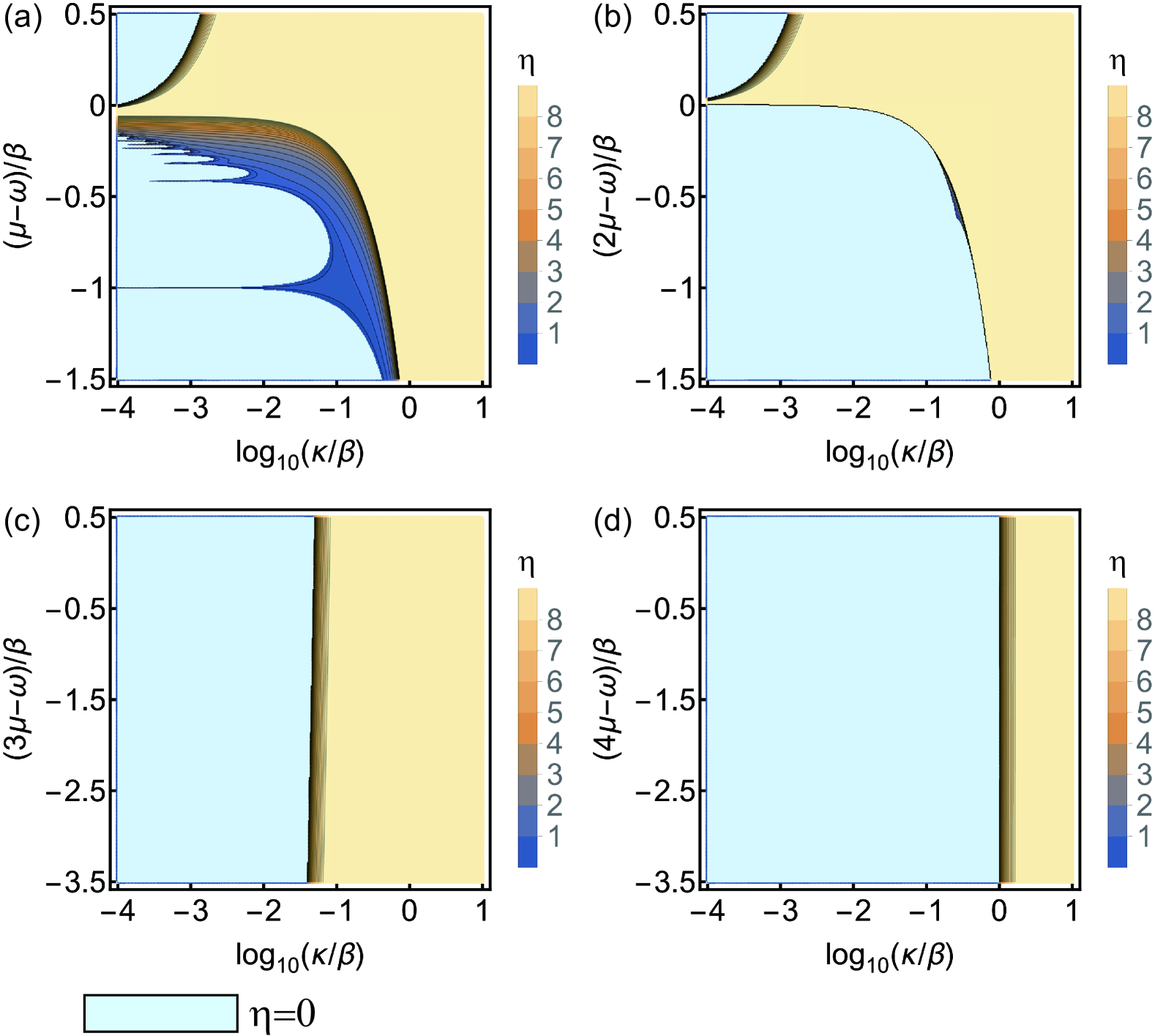
Figure 1: The contour plots of $\psi={\psi}_{E_{\rm min}}$ that gives the minimum energy of $\hat{H}_{\mbox{\scriptsize MF}}$ for $l=1$ (a), $2$ (b), $3$ (c), and $4$ (d) respectively with $\Delta=\omega-\epsilon=0$, $\mu/\beta=1$, and $z=2$. The order parameter is equal to zero ($\psi=0$) in the light blue area.

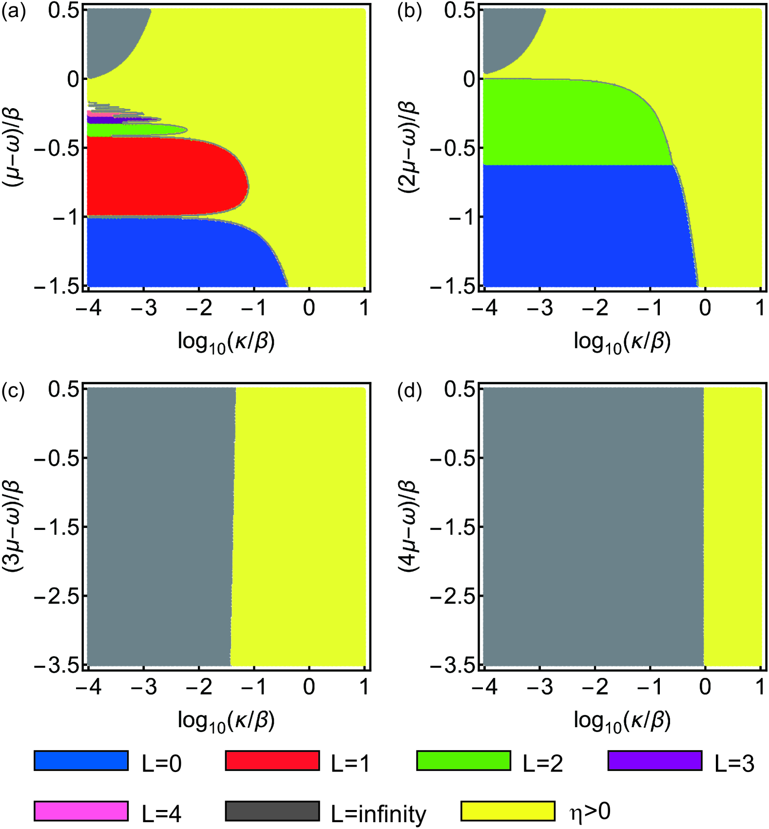
Figure 2: Phase diagrams for $l=1$ (a), $2$ (b), $3$ (c), and $4$ (d) respectively, classified by eigenvalues $L$ with $\Delta=0$, $\mu/\beta=1$, and $z=2$. The blue, red, green, purple, pink, and gray regions have eigenvalues $L=0,1,2,3,4$, and $\infty$, respectively, with $\psi=0$. The white regions represent that $5\leq L<\infty$ with $\psi=0$. The yellow areas represent $\psi>0$.

Now let us consider the situation in which the system is in the MI phase. In this case (because of $\psi=0$) the Hamiltonian simplifies to

$$\hat{H}^{\prime}_{\mbox{\scriptsize MF}}=\hat{H}_{\mbox{\scriptsize mpJC}}-\hbar\mu\hat{L}.$$ (12)

Here the operator $\hat{L}$ represents the sum of the number of excited atoms and photons in the resonant mode for $l=1$. The eigenvalue $L$ is a conserved quantity $\forall l$ because $[\hat{H}_{\mbox{\scriptsize mpJC}},\hat{L}]=0$. This means we can classify the areas of the MI phase according to this conserved quantity.

In Fig. 2, we classify the regions of the MI phase by the eigenvalue $L$ for $l=1,2,3$, and $4$, respectively. Looking at Fig. 2(a), we note that we can divide the region of the MI phase into parts of $L=0,1,2,...,\infty$ for $l=1$ (the single-photon JCHM). For $L=0$, the wave function of the lowest energy is given by $|g\rangle_{\mbox{\scriptsize A}}|0\rangle_{\mbox{\scriptsize P}}$, where $\{|g\rangle_{\mbox{\scriptsize A}},|e\rangle_{\mbox{\scriptsize A}}\}$ are atomic ground and excited states and $\{|n\rangle_{\mbox{\scriptsize P}}:n=0,1,2,...\}$ are the Fock states of the photons. For $L=1$ and $2$, the wave functions of the lowest energy are given by $(1/\sqrt{2})(|g\rangle_{\mbox{\scriptsize A}}|1\rangle_{\mbox{\scriptsize P}}-|e\rangle_{\mbox{\scriptsize A}}|0\rangle_{\mbox{\scriptsize P}})$ and $(1/\sqrt{2})(|g\rangle_{\mbox{\scriptsize A}}|2\rangle_{\mbox{\scriptsize P}}-|e\rangle_{\mbox{\scriptsize A}}|1\rangle_{\mbox{\scriptsize P}})$, respectively. Here, we draw attention to the fact that the wave functions are given by $|\varphi_{-}\rangle=(1/\sqrt{2})(|g\rangle_{\mbox{\scriptsize A}}|L\rangle_{\mbox{\scriptsize P}}-|e\rangle_{\mbox{\scriptsize A}}|L-1\rangle_{\mbox{\scriptsize P}})$ but not $|\varphi_{+}\rangle=(1/\sqrt{2})(|g\rangle_{\mbox{\scriptsize A}}|L\rangle_{\mbox{\scriptsize P}}+|e\rangle_{\mbox{\scriptsize A}}|L-1\rangle_{\mbox{\scriptsize P}})$ for $L=1$ and $2$. This is because an expectation value of the interaction term in $\hat{H}_{\mbox{\scriptsize mpJC}}$ given by Eq. (9) is equal to $\langle\varphi_{\pm}|\hbar\beta(\hat{\sigma}_{+}\hat{a}+\hat{\sigma}_{-}\hat{a}^{\dagger})|\varphi_{\pm}\rangle=\pm\hbar\beta$. Thus, the energy of $|\varphi_{-}\rangle$ is smaller than that of $|\varphi_{+}\rangle$ if $\beta>0$. This fact is applicable for the $l$-photon JCHM with $l=2,3$, and $4$, as well.

In the gray area of Fig. 2(a), we obtain $L=M$ and the wave function of the lowest energy $(1/\sqrt{2})(|g\rangle_{\mbox{\scriptsize A}}|M\rangle_{\mbox{\scriptsize P}}-|e\rangle_{\mbox{\scriptsize A}}|M-1\rangle_{\mbox{\scriptsize P}})$ if we compute the superfluid order parameter $\psi$ with a $(2M+1)$-dimensional Hilbert space spanned by $\{|g\rangle_{\mbox{\scriptsize A}}|0\rangle_{\mbox{\scriptsize P}},|e\rangle_{\mbox{\scriptsize A}}|0\rangle_{\mbox{\scriptsize P}},|g\rangle_{\mbox{\scriptsize A}}|1\rangle_{\mbox{\scriptsize P}},|e\rangle_{\mbox{\scriptsize A}}|1\rangle_{\mbox{\scriptsize P}},...,|g\rangle_{\mbox{\scriptsize A}}|M-1\rangle_{\mbox{\scriptsize P}},|e\rangle_{\mbox{\scriptsize A}}|M-1\rangle_{\mbox{\scriptsize P}},|g\rangle_{\mbox{\scriptsize A}}|M\rangle_{\mbox{\scriptsize P}}\}$. As $M\to\infty$, the eigenvalue $L$ diverges to infinity. Thus, in the gray area, we obtain $\psi=0$ and $L=\infty$, and we consider that the photons are localized in each site and its number of the photons becomes infinite. Because an infinite number of the photons occupies the state of the lowest energy, we associate that with the BEC phase.

Examining Fig. 2(b) in more detail, we note that we can divide the region of $\psi=0$ into three parts, $L=0,2$, and $\infty$ for $l=2$ (the two-photon JCHM). This means all three phases appear, the MI, BEC, and superfluid phases. For $L=0,2$, and $\infty$, the wave functions of the lowest energy are given by $|g\rangle_{\mbox{\scriptsize A}}|0\rangle_{\mbox{\scriptsize P}}$, $c_{0}|g\rangle_{\mbox{\scriptsize A}}|2\rangle_{\mbox{\scriptsize P}}+c_{1}|e\rangle_{\mbox{\scriptsize A}}|0\rangle_{\mbox{\scriptsize P}}$ and $(1/\sqrt{2})(|g\rangle_{\mbox{\scriptsize A}}|M\rangle_{\mbox{\scriptsize P}}-|e\rangle_{\mbox{\scriptsize A}}|M-2\rangle_{\mbox{\scriptsize P}})$ with $M\to\infty$, respectively, where the values of $c_{0}$ and $c_{1}$ depend on $\beta/\omega$.

Next in the graph of Fig. 2(b), the boundary point between the blue and green regions is given by $(2\mu-\omega)/\beta=-0.6180$ for $\log_{10}(\kappa/\beta)=-4$. The smallest value of $(2\mu-\omega)/\beta$ for the gray area with $\log_{10}(\kappa/\beta)=-4$ is given by $0.00116$ in Fig. 2(b).

Now exploring Figs. 2(c), (d), we oberve that $L$ diverges to infinity in the region of $\psi=0$ for $l=3$ and $4$. Thus, for $l=3$ and $4$, we can regard those areas as the BEC phase. The wave functions of the BEC phase in Figs. 2(c), (d) are given by $(1/\sqrt{2})(|g\rangle_{\mbox{\scriptsize A}}|M\rangle_{\mbox{\scriptsize P}}-|e\rangle_{\mbox{\scriptsize A}}|M-3\rangle_{\mbox{\scriptsize P}})$ and $(1/\sqrt{2})(|g\rangle_{\mbox{\scriptsize A}}|M\rangle_{\mbox{\scriptsize P}}-|e\rangle_{\mbox{\scriptsize A}}|M-4\rangle_{\mbox{\scriptsize P}})$ with $M\to\infty$ for $l=3$ and $4$, respectively. Therefore, we conclude that the MI phases of finite $L=1,3,4,...$ do not appear in Fig. 1(b) for the two-photon JCHM. Moreover, the MI phases do not arise in Fig. 1(c),(d) for the three- and four-photon JCHMs. We give intuitive explanations of those observations in Sec. V.

From the above considerations, we find three phases of the multiphoton JCHMs, the MI, BEC, and superfluid phases. Here, we examine how sharp the transitions between these phases are. Figure 3 show plots of the minimum energies as functions of $\log_{10}(\kappa/\beta)$ for $\Delta=0$, $\mu/\beta=1$, $z=2$, and $l=1$ (the single-photon JCHM) with choosing specific values of $(\mu-\omega)/\beta$.

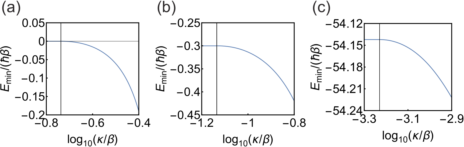
Figure 3: Plots of the minimum energies $E_{\mbox{\scriptsize min}}/(\hbar\beta)$ as functions of $\log_{10}(\kappa/\beta)$ for $\Delta=0$, $\mu/\beta=1$, and $z=2$ for the single-photon JCHM ($l=1$). Here we assume the $(2M+1)$-dimensional Hilbert space with $M=200$. The three subfigures correspond to (a) $(\mu-\omega)/\beta=-1.2$, $L=0$, (b) $(\mu-\omega)/\beta=-0.7$, $L=1$, (c) $(\mu-\omega)/\beta=0.2$, $L=\infty$. The critical points between $\psi=0$ and $\psi>0$ are given by $\log_{10}(\kappa/\beta)=-0.737$, $-1.14$, and $-3.23$ for (a), (b), and (c), respectively. Near the critical points in the plots, ratios of differences of $E_{\mbox{\scriptsize min}}/(\hbar\beta)$ to differences of $\log_{10}(\kappa/\beta)$ are given by $\Delta E_{\mbox{\scriptsize min}}/[(\hbar\beta)\Delta\log_{10}(\kappa/\beta)]=0.40$, $0.30$, and $0.22$ for (a), (b), and (c), respectively.

Here we consider the $(2M+1)$-dimensional Hilbert space which is spanned by the orthonormal basis $\{|g\rangle_{\mbox{\scriptsize A}}|0\rangle_{\mbox{\scriptsize P}},|e\rangle_{\mbox{\scriptsize A}}|0\rangle_{\mbox{\scriptsize P}},|g\rangle_{\mbox{\scriptsize A}}|1\rangle_{\mbox{\scriptsize P}},|e\rangle_{\mbox{\scriptsize A}}|1\rangle_{\mbox{\scriptsize P}},...,|g\rangle_{\mbox{\scriptsize A}}|M-1\rangle_{\mbox{\scriptsize P}},|e\rangle_{\mbox{\scriptsize A}}|M-1\rangle_{\mbox{\scriptsize P}},|g\rangle_{\mbox{\scriptsize A}}|M\rangle_{\mbox{\scriptsize P}}\}$ with $M=200$. For Figs. 3(a)-3(c), values of $\Delta E_{\mbox{\scriptsize min}}/[(\hbar\beta)\Delta\log_{10}(\kappa/\beta)]$, that is, ratios of differences of $E_{\mbox{\scriptsize min}}/(\hbar\beta)$ to differences of $\log_{10}(\kappa/\beta)$, near the critical points are of order $10^{-1}$. Thus, we can regard all of the transitions as sharp. The values of $|E_{\mbox{\scriptsize min}}|/(\hbar\beta)$ are of order $10^{-1}$ for the phase transitions between the MI and superfluid phases. By contrast, $|E_{\mbox{\scriptsize min}}|/(\hbar\beta)$ is larger than $50$ and it diverges to infinity for $M\to\infty$ for the phase transitions between the BEC and superfluid phases. Because $\Delta E_{\mbox{\scriptsize min}}/[(\hbar\beta)\Delta\log_{10}(\kappa/\beta)]$ is of order $10^{-1}$ and $|E_{\mbox{\scriptsize min}}|/(\hbar\beta)$ is infinite, we expect the BEC phase is not stable.

V The presence or absence MI phases in the multiphoton JCHMs

Examining Fig. 2(b) we observe that the MI phases of $L=1$ and $3$ do not arise in the two-photon JCHM. Is there a simple explanation why? Let us assume that $\psi=0$ holds because we want to concentrate on the behavior of the system in the MI and BEC phases. For the $l$-photon JCHM with $\psi=0$, we can write the dimensionless Hamiltonian derived from Eqs. (8-10) in the form,

$$\tilde{H}^{(l)}=\tilde{\epsilon}\hat{\sigma}_{+}\hat{\sigma}_{-}+\tilde{\omega}\hat{a}^{\dagger}\hat{a}+\hat{\sigma}_{+}\hat{a}^{l}+\hat{\sigma}_{-}(\hat{a}^{\dagger})^{l}-\tilde{\mu}\hat{L},$$ (13)

$$\hat{L}=l\hat{\sigma}_{+}\hat{\sigma}_{-}+\hat{a}^{\dagger}\hat{a},$$ (14)

where $\tilde{\epsilon}=\epsilon/\beta$, $\tilde{\omega}=\omega/\beta$, and $\tilde{\mu}=\mu/\beta$. As mentioned in Sec. III, this simplified Hamiltonian is valid for $\kappa/\beta\ll 1$.

Now let us concentrate on cases of $l=2$ two-photon JCHM. First, we consider a state with $L=0$. It is equal to $|g\rangle_{\mbox{\scriptsize A}}|0\rangle_{\mbox{\scriptsize P}}$ and its dimensionless energy is given by $\tilde{E}^{(2)}_{0}=0$. Second, we consider a state with $L=1$ which can be represented by $|g\rangle_{\mbox{\scriptsize A}}|1\rangle_{\mbox{\scriptsize P}}$ with its dimensionless energy given by $\tilde{E}^{(2)}_{1}=\tilde{\omega}$. This shows that $\tilde{E}^{(2)}_{0}<\tilde{E}^{(2)}_{1}$ holds $\forall\tilde{\omega}>0$ and the phase of $\psi=0$ and $L=1$ cannot be realized. Thus, the MI phase of $L=1$ does not appear in Fig. 2(b). Third if we consider a state with $L(\geq l)$ for the $l$-photon JCHM, it can be represented by a superposition of $|g\rangle_{\mbox{\scriptsize A}}|L\rangle_{\mbox{\scriptsize P}}$ and $|e\rangle_{\mbox{\scriptsize A}}|L-l\rangle_{\mbox{\scriptsize P}}$. Taking $\{|g\rangle_{\mbox{\scriptsize A}}|L\rangle_{\mbox{\scriptsize P}},|e\rangle_{\mbox{\scriptsize A}}|L-l\rangle_{\mbox{\scriptsize P}}\}$ as an orthonormal basis, we describe $\tilde{H}^{(l)}$ in the following $2\times 2$ matrix form:

$$\tilde{H}^{(l)}=\left(\begin{array}[]{cc}\tilde{\epsilon}+(L-l)\tilde{\omega}-L\tilde{\mu}&\sqrt{L!/(L-l)!}\\ \sqrt{L!/(L-l)!}&L\tilde{\omega}-L\tilde{\mu}\\ \end{array}\right),$$ (15)

The eigenvalues of $\tilde{H}^{(l)}$ with $\Delta=\omega-\epsilon=0$ and $\tilde{\mu}=1$ are

$$\tilde{E}^{(l)}_{L,\pm}=\frac{1}{2}[-2L+(2L-l+1)\tilde{\omega}\pm\sqrt{4L!/(L-l)!+(l-1)^{2}\tilde{\omega}^{2}}].$$ (16)

Now by letting $l=2$ and $L=2$ we have

$$\tilde{E}^{(2)}_{2,-}=\frac{1}{2}(-4+3\tilde{\omega}-\sqrt{8+\tilde{\omega}^{2}}),$$ (17)

which is less than zero for $\tilde{\omega}<(1/2)(3+\sqrt{5})\simeq 2.6180$. Thus, if $(2\mu-\omega)/\beta<-0.6180$, the $L=0$ MI phase of emerges. By contrast, if $(2\mu-\omega)/\beta>-0.6180$, the $L=2$ MI phase arises. This can be observed Fig. 2(b). Substituting $l=2$ and $L=3$ into Eq. (16), we obtain

$$\tilde{E}^{(2)}_{3,\pm}=\frac{1}{2}(-6+5\tilde{\omega}\pm\sqrt{24+\tilde{\omega}^{2}}).$$ (18)

Now $\tilde{E}^{(2)}_{3,-}=\tilde{E}^{(2)}_{2,-}$ holds for $\tilde{\omega}\simeq 1.9215$. Hence, if $(2\mu-\omega)/\beta>0.0785$, the MI phase of $L=3$ could emerge. However, this situation is forbidden because of the following fact. Let us consider a case for large $L$. As

$$\lim_{L\to\infty}\frac{1}{L}\tilde{E}^{(2)}_{L,-}=\tilde{\omega}-2,$$ (19)

$\tilde{E}_{L,-}^{(2)}\to-\infty$ and $\tilde{E}_{L,-}^{(2)}<\tilde{E}_{3,-}^{(2)}$ hold for $\tilde{\omega}<2$ under $L\to\infty$. The BEC phase must appear for $\tilde{\omega}<2$, that is $(2\mu-\omega)/\beta>0$. This means the MI phase of $L=3$ does not arise. On the contrary, the BEC phase appears.

Now is there a similar explanation for why the MI phases cannot be observed in the three- and four-photon JCHMs. Let us set $l=3$ and consider a state whose conserved quantity is equal to $L$. We obstain

$$\lim_{L\to\infty}\frac{\tilde{E}^{(3)}_{L,-}}{L^{3/2}}=-1\quad\forall\tilde{\omega}.$$ (20)

Thus, the superposition of $|g\rangle_{\mbox{\scriptsize A}}|L\rangle_{\mbox{\scriptsize P}}$ and $|e\rangle_{\mbox{\scriptsize A}}|L-3\rangle_{\mbox{\scriptsize P}}$ are the lowest energy states with $\tilde{E}_{L,-}^{(3)}\to-\infty$ $\forall\omega$ in the limit of $L\to\infty$. As such we may conclude that the BEC phase appears and the MI phases do not arises for the three-photon JCHM. Similar behaviour occurs in the our-photon JCHM case.

VI Conclusion

In this work we investigated the quantum phase transitions of the $l$-photon JCHMs for $l=1,2,3,4$ using the mean-field approximation. This enabled us to establish phase diagrams for the multiphoton Jaynes-Cummings-Hubbard model which clearly show the Mott insulator, superfluid and BEC phases. We observed that all three phases arise in the single- and two-photon JCHMs phase diagrams. However, although the single-photon JCHM has the MI phases with finite $L=0,1,2,3,...$, the two-photon JCHM has the MI phase only for $L=0$ and $2$. Further the three- and four-JCHMs only shows the superfluid and BEC phases but not the MI phase. The observation that the BEC occurs in some areas of the phase diagrams for the multiphoton JCHMs is interesting and may provide motivation for new experiments in this regime.

References

- [1] M. Toda, R. Kubo, and N. Saitô, Statistical Physics I: Equilibrium Statistical Mechanics, 2nd ed. (Springer-Verlag, Berlin, 1992).
- [2] M. Vojta, ‘Quantum phase transitions’, Rep. Prog. Phys. 66, 2069 (2003).
- [3] M. Greiner, O. Mandel, T. Esslinger, T. W. Hänsch, and I. Bloch, ‘Quantum phase transition from a superfluid to a Mott insulator in a gas of ultracold atoms’, Nature 415, 39 (2002).
- [4] M. P. A. Fisher, P. B. Weichman, G. Grinstein, and D. S. Fisher, ‘Boson localization and the superfluid-insulator transition’, Phys. Rev. B 40, 546 (1989).
- [5] D. van Oosten, P. van der Straten, and H. T. C. Stoof, ‘Mott insulators in an optical lattice with high filling factors’, Phys. Rev. A 67, 033606 (2003).
- [6] F. Alet and E. S. Sørensen, ‘Generic incommensurate transition in the two-dimensional boson Hubbard model’, Phys. Rev. B 70, 024513 (2004).
- [7] M. J. Hartmann, F. G. S. L. Brandão, and M. B. Plenio, ‘Strongly interacting polaritons in coupled arrays of cavities’, Nat. Phys. 2, 849 (2006).
- [8] . D. G. Angelakis, M. F. Santos, and S. Bose, ‘Photon-blockade-induced Mott transitions and spin models in coupled cavity arrays’, Phys. Rev. A 76, 031805(R) (2007).
- [9] A. D. Greentree, C. Tahan, J. H. Cole, and L. C. L. Hollenberg, ‘Quantum phase transitions of light’, Nat. Phys. 2, 856 (2006).
- [10] J. Quach, M. I. Makin, C.-H. Su, A. D. Greentree, and L. C. L. Hollenberg, ‘Band structure, phase transitions, and semiconductor analogs in one-dimensional solid light systems’, Phys. Rev. A 80, 063838 (2009).
- [11] A. Mering, M. Fleischhauer, P. A. Ivanov, and K. Singer, ‘Analytic approximations to the phase diagram of the Jaynes-Cummings-Hubbard model’, Phys. Rev. A 80, 053821 (2009).
- [12] S. Schmidt and G. Blatter, ‘Strong coupling theory for the Jaynes-Cummings-Hubbard model’, Phys. Rev. Lett. 103, 086403 (2009).
- [13] M. Hohenadler, M. Aichhorn, S. Schmidt, and L. Pollet, ‘Dynamical critical exponent of the Jaynes-Cummings-Hubbard model’, Phys. Rev. A 84, 041608(R) (2011).
- [14] D. Rossini and R. Fazio, ‘Mott-insulating and glassy phases of polaritons in 1D arrays of coupled cavities’, Phys. Rev. Lett. 99, 186401 (2007).
- [15] M. I. Makin, J. H. Cole, C. Tahan, L. C. L. Hollenberg, and A. D. Greentree, ‘Quantum phase transitions in photonic cavities with two-level systems’, Phys. Rev. A 77, 053819 (2008).
- [16] A. Tomadin and R. Fazio, ‘Many-body phenomena in QED-cavity arrays’, JOSA B 27, A130 (2010).
- [17] E. T. Jaynes and F. W. Cummings, ‘Comparison of quantum and semiclassical radiation theories with application to the beam maser’, Proc. IEEE 51, 89 (1963).
- [18] B. W. Shore and P. L. Knight, ‘The Jaynes-Cummings model’, J. Mod. Opt. 40, 1195 (1963).
- [19] S. Felicetti, D. Z. Rossatto, E. Rico, E. Solano, and P. Forn-Díaz, ‘Two-photon quantum Rabi model with superconducting circuits’, Phys. Rev. A 97, 013851 (2018).
- [20] S. Felicetti, J. S. Pedernales, I. L. Egusquiza, G. Romero, L. Lamata, D. Braak, and E. Solano, ‘Spectral collapse via two-phonon interactions in trapped ions’, Phys. Rev. A 92, 033817 (2015).
- [21] R. Puebla, M.-J. Hwang, J. Casanova, and M. B. Plenio, ‘Protected ultrastrong coupling regime of the two-photon quantum Rabi model with trapped ions’, Phys. Rev. A 95, 063844 (2017).
- [22] C. Kittel, Introduction to Solid State Physics, 7th ed. (John Wiley & Sons, Inc., New York, 1996).
- [23] R. P. Feynman, R. B. Leighton, and M. Sands, The Feynman Lectures on Physics, Vol. III: Quantum Mechanics, the definitive edition (Addison-Wesley Pub. Co., Reading, Massachusetts, 2006).
- [24] K. Sheshadri, H. R. Krishnamurthy, R. Pandit, and T. V. Ramakrishnan, ‘Superfluid and insulating phases in an interacting-boson model: mean-field theory and the RPA’, Europhys. Lett. 22, 257 (1993).