Approximating Opaque Top-k Queries

Abstract.

Combining query answering and data science workloads has become prevalent. An important class of such workloads is top-k queries with a scoring function implemented as an opaque UDF—a black box whose internal structure and scores on the search domain are unavailable. Some typical examples include costly calls to fuzzy classification and regression models. The models may also be changed in an ad-hoc manner. Since the algorithm does not know the scoring function’s behavior on the input data, opaque top-k queries become expensive to evaluate exactly or speed up by indexing. Hence, we propose an approximation algorithm for opaque top-k query answering. Our proposed solution is a task-independent hierarchical index and a novel bandit algorithm. The index clusters elements by some cheap vector representation then builds a tree of the clusters. Our bandit is a diminishing returns submodular epsilon-greedy bandit algorithm that maximizes the sum of the solution set’s scores. Our bandit models the distribution of scores in each arm using a histogram, then targets arms with fat tails. We prove that our bandit algorithm approaches a constant factor of the optimal algorithm. We evaluate our standalone library on large synthetic, image, and tabular datasets over a variety of scoring functions. Our method accelerates the time required to achieve nearly optimal scores by up to an order of magnitude compared to exhaustive scan while consistently outperforming baseline sampling algorithms.

1. Introduction

Intermixing opaque user defined functions (UDF) with query answering has become an important workload for performing data science on unstructured text, images, and tabular data (Foufoulas and Simitsis, 2023). An opaque UDF is a black-box function whose semantics and internal structure nor its scores on the database are available a priori (He et al., 2020). They are invoked in stand-alone code bases (Spiegelberg et al., 2021; He et al., 2020, 2024) or intermixed with SQL queries (He et al., 2020; Anderson and Cafarella, 2016; He et al., 2024; Sikdar and Jermaine, 2020). Opaque UDFs are typically written in conventional programming languages and they increasingly involve calls to machine learning models (Foufoulas and Simitsis, 2023; Spiegelberg et al., 2021; Dai et al., 2024; Grulich et al., 2021), as emerging academic and industry systems integrate ad-hoc model training and inference into databases with declarative interfaces. For example, users may train models on-the-fly to predict missing values (Hasani et al., 2019; Jin et al., 2024; Zhao et al., 2024) or prompt large language models (LLMs) (Dai et al., 2024; Anderson et al., 2024; Liu et al., 2024; Patel et al., 2024; DataBricks, 2024; Sukumaran, 2023) via an SQL extension.

1.1. Opaque Top-k Queries

Opaque top-$k$ queries rank elements in a database by an opaque scoring function, and return the $k$ highest scoring elements.

SELECT * FROM vehicleListings
ORDER BY ValuationUDF(listing) LIMIT 250;

For example, an analyst may want to retrieve 250 current vehicle listings that have the highest predicted valuations by applying a price prediction ML model on a database of listings.

Traditional top-$k$ query answering literature generally assumes certain properties on scoring functions (Ilyas et al., 2008; Fagin et al., 2001). For example, the family of Threshold Algorithm (TA) variants typically assume that the scoring function is a monotone aggregate (Fagin, 1996; Fagin et al., 2001; Ilyas et al., 2008; Bruno and Wang, 2007; Shmueli-Scheuer et al., 2009). Another class of scoring functions is similarity functions, such as inner product of vector representations (Pan et al., 2024). These function classes are prevalent yet suffer from limited expressivity, potentially losing complex user intent.

Arbitrary UDFs, however, pose fundamental challenges to top-$k$ query evaluation. First, they may be difficult to analyze, as they involve imperative programming languages and ML models. Existing methods increase programmer burden (Spiegelberg et al., 2021) or limit the scope (Hagedorn et al., 2021) in order to expose the internals of the UDF to the compiler. Second, they may be expensive to run—foundation models are the extreme case (Dai et al., 2024; Liu et al., 2024; DataBricks, 2024; Sukumaran, 2023). Hence, an exhaustive scan is not attractive. Third, the scores given by the function may change over time, if the scoring function is a continually learning model (De Lange et al., 2021) or if the score depends on some external factor, like a user-specified label or prompt. As such, it is hard to build a sorted index over the elements’ scores or apply the existing approximate nearest neighbor search techniques (Wang et al., 2021). Concretely, consider the following scenario.

Example 1.1.

Analyst Alice is developing an in-house model to predict the market prices of used vehicles. The model is updated frequently to adapt to changing market preferences. She is interested in identifying which listings have the highest predicted valuations, as this would help her company target its most valuable customers. To achieve this, she trains a gradient-boosted decision tree model for tabular regression (Chen and Guestrin, 2016). This UDF is an opaque scoring function: it invokes a model and incurs significant inference latency, and it is constantly evolving. Alice then issues a top-$k$ query using this UDF to find the 250 highest-valued listings from a dataset of hundreds of thousands. As she continues to refine the model, she will repeatedly issue new top-$k$ queries. Since she wants to interactively analyze the dataset and the models, she is willing to sacrifice some quality for reduced latency.

Traditional methods are unsatisfactory for the query given in Example 1.1. Conventional data engines such as Spark or PostgreSQL treat UDFs as a black box, and will execute the UDF exhaustively on all data points (He et al., 2020; Cao and Wang, 2004). This is not viable when the search domain is very large, each invocation of the model is costly, or the user does not need the exact top-$k$ solution. Taking a sample of the search domain is also viable, but degrades in quality when only a small subset of the elements have high scores. Uniform sampling, in the worst case, requires a sample size of $n(1-\varepsilon)$, where $n$ is the number of data points and $\varepsilon$ is approximation tolerance. Specialized algorithms for limited classes of scoring functions and indexes are not applicable, either.

A recent body of work studied how to statistically optimize opaque UDF queries. However, existing methods are limited to other types of queries, such as feature engineering (Anderson and Cafarella, 2016), selection (He et al., 2020; Dai et al., 2024), aggregation (Dai et al., 2024), and queries with partially obscured predicates (Sikdar and Jermaine, 2020). To the best of our knowledge, no prior work studied statistical optimization for opaque top-$k$ queries.

A method for approximate opaque top-$k$ query execution has to balance conflicting objectives. It should be applicable across a wide variety of opaque scoring functions. It should not incur significant execution-time overhead in the worst-case scenario. It should be amenable to batched execution to maximize lower-level optimization opportunities. Finally, its performance-over-time curve should be close to optimal, and consistently better than random sampling.

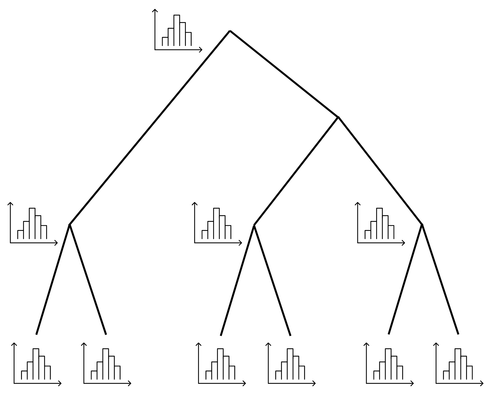
(a) Hierarchical cluster with
histogram sketches.

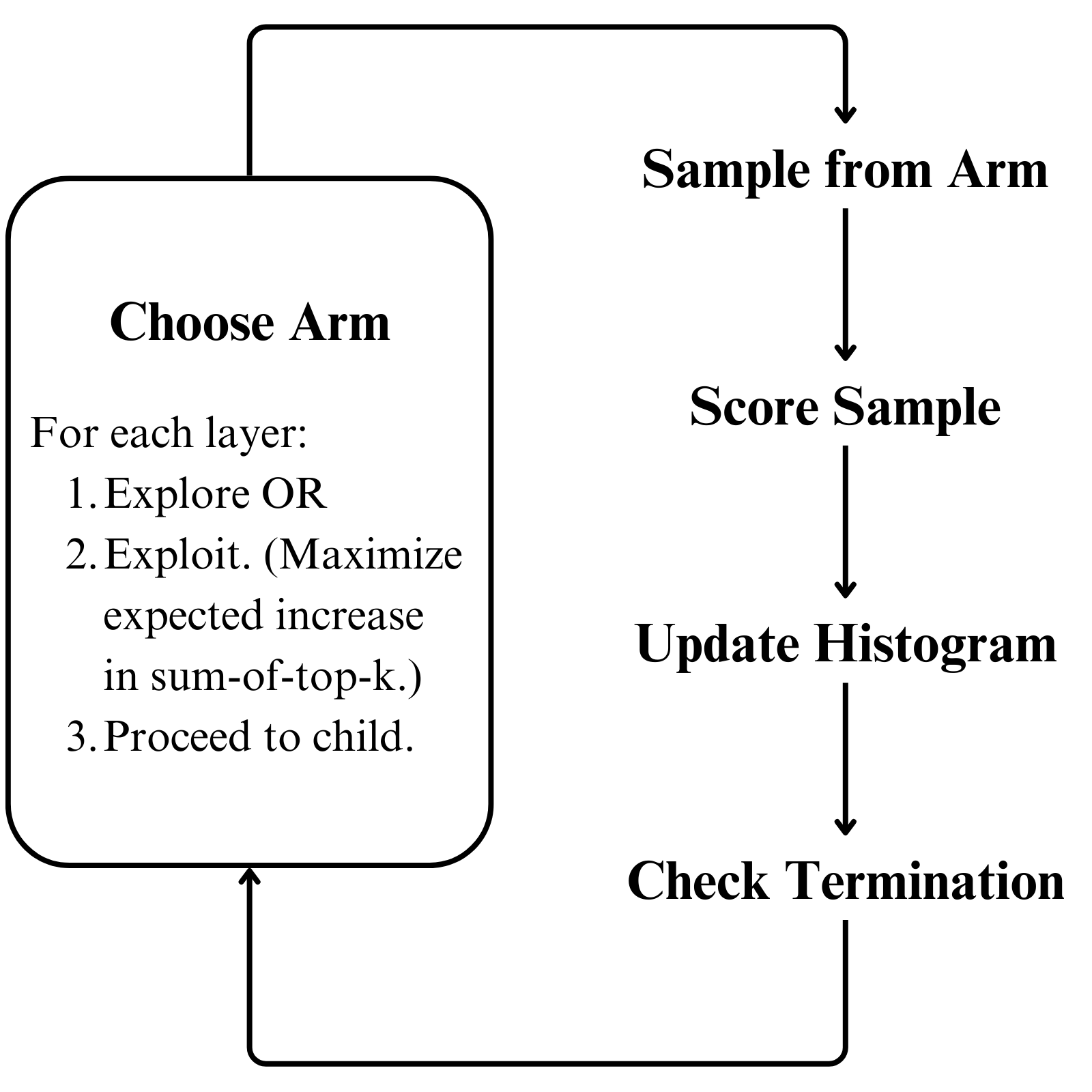
(b) Each iteration of our
bandit algorithm.

Figure 1. A high-level overview of our proposed solution during indexing and query execution.

Left: A non-balanced binary tree where each node, including leaves, have a histogram sketch attached. Right: The logical loop of one iteration of our bandit algorithm, which repeates: choose arm, sample from arm, score sample, update histogram, and check termination.

1.2. Solution Sketch

Our proposed solution, as illustrated in Figure 1b, consists of a tree index and a novel bandit algorithm. The tree index hierarchically clusters data at preprocessing time before any opaque top-$k$ queries.

We adopt the VOODOO index from He et al. (He et al., 2020). This index vectorizes each element using a cheap heuristic, applies $k$-means clustering to the vectors, and then performs agglomerative clustering on the cluster centroids.

Our main technical contribution is the query execution algorithm. We abstract the problem of sampling over a collection of heterogeneous clusters for top-$k$ queries as a stochastic diminishing returns (DR) submodular bandit problem (Soma et al., 2014; Asadpour and Nazerzadeh, 2016). In this problem setting, there are three classes of algorithms: offline, non-adaptive, and adaptive. The optimal offline algorithm is the theoretical best-case scan when the insertion order of the data is ideal. Adaptive algorithms change their behavior based on the realizations of random samples; non-adaptive algorithms do not. Prior work established gaps between the three classes (Hellerstein et al., 2015; Asadpour and Nazerzadeh, 2016). We design an algorithm that performs close to the optimal adaptive, as illustrated in Figure 2.

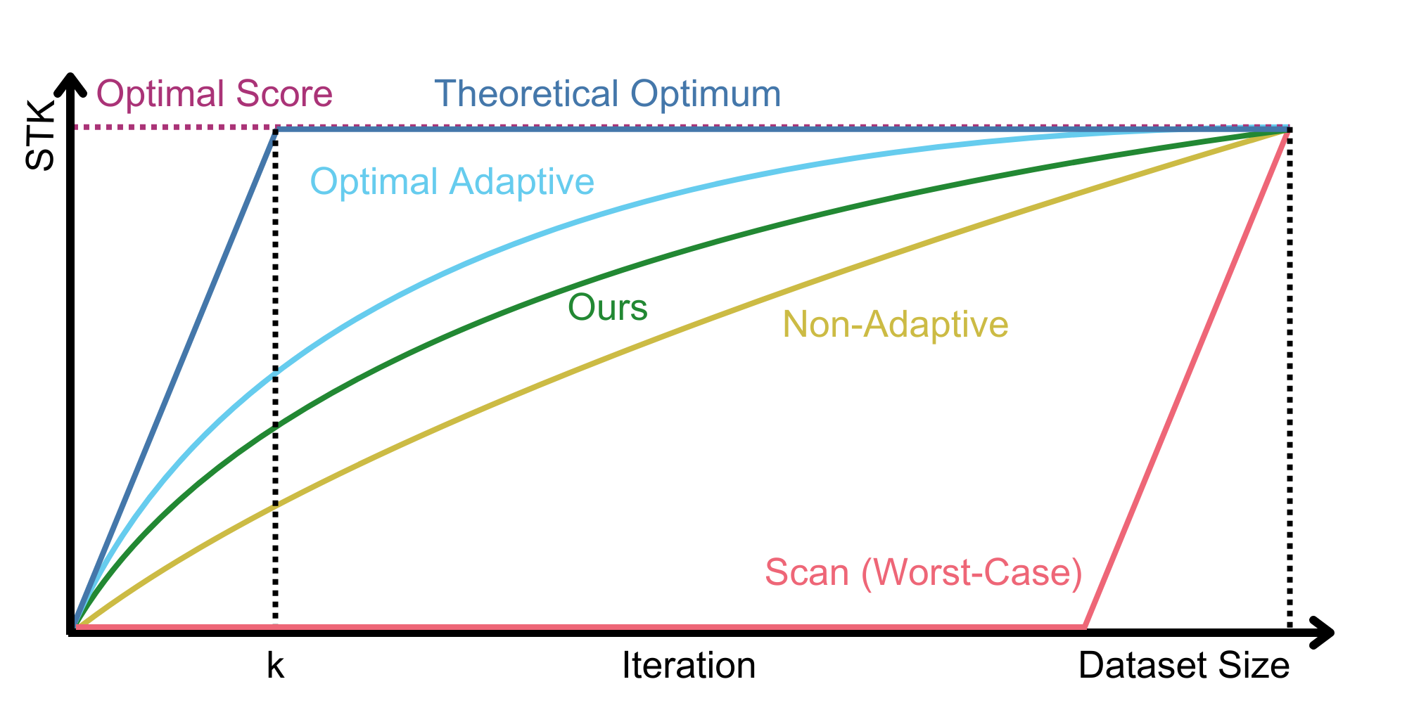
Figure 2. Visualizing the relative performance of various algorithms. $x$-axis is the number of iterations (i.e. scoring function calls) and the $y$-axis indicates the quality of results in terms of the sum of top-$k$ scores (STK).

The optimal score in terms of STK is some unknown constant. If the elements are ordered in the best or the worst case, Scan achieves the optimal score after just $k$ iterations, or as late as after $n-k$ iterations. The optimal adaptive algorithm is closest to the theoretical optimum, followed by Ours and non-adaptive sampling algorithms.

Our main contributions are summarized below.

1. We study the problem of approximating opaque top-$k$ queries. We formalize query answering over the index structure as a DR-submodular bandit problem.

2. We propose a histogram-based $\varepsilon$-greedy bandit algorithm.

3. We prove approximation guarantees for the objective of maximizing the total utility of the solution, given by its sum of scores. When the scoring domain is non-negative, discrete and finite, our algorithm’s expected utility is lower bounded by $(1-\exp(-1-1/2T))\text{OPT}-O(T^{2/3})$ at iteration limit $T$, which approaches 63% of the optimal adaptive algorithm.

4. When the scoring distribution is an arbitrary non-negative interval, we describe a histogram maintenance strategy that improves flexibility and accuracy, and fallback strategies that improve practical performance.

5. We implement our solution as a standalone library and perform extensive experiments on large synthetic, image, and tabular datasets over a variety of scoring functions.

The remainder of this paper is organized as follows. In § 2, we formally define the concrete and abstract problems. § 3 presents our bandit algorithm. In § 4, we establish the theoretical guarantees. § 5 reports the experimental results. We discuss related work in § 6. Finally, we conclude with a discussion in § 7 and 8.

2. Problem Definition

This section defines two related problems: the first is the concrete problem of answering opaque top-$k$ queries, and the second is an abstract bandit problem that assumes an index.

Refer to Table 1 for the precise definition of notations.

Notation	Definition
$T$	Iteration limit. Unknown a priori.
$t$	Current iteration count.
$S_{t}$	Set of scores of the running solution at iteration $t$ or the solution set itself.
$k$	Cardinality LIMIT on the query result.
$\mathcal{M}(\mathcal{X})$	The set of all multisets over some domain $\mathcal{X}$.
$\mathcal{X}$	The domain of all legal elements.
$D$	The target dataset.
$n$	Number of elements in $D$.
$f$	Scoring function.
$L$	Number of clusters in some clustering of $D$.
$\mathcal{D}_{l}$	Distribution of scores of elements in the $l^{\text{th}}$ cluster.
$p(x|\mathcal{D}_{l})$	Probability of sampling outcome $x$ from $D_{l}$.
$S_{(k)}$	$k^{\text{th}}$ largest element of some (multi)set $S$.
$\text{STK}(S)$	Sum of the $k$ largest elements in (multi)set $S$.
OPT	$\mathbb{E}[STK(S_{t})]$ for the optimal adaptive algorithm.
$\Delta_{t}$	$\text{STK}(S_{t})-\text{STK}(S_{t-1})$.
$\mathbb{E}[\Delta_{t,l}]$	Expected $\Delta_{t}$ after sampling from $\mathcal{D}_{l}$.
$l_{t}$	Cluster chosen by our algorithm at iteration $t$.
$B$	Number of buckets in histogram sketches.
$\alpha$	Initial maximum range of the histograms.
$\beta$	Re-binning overestimation parameter.
$F$	Frequency to check fallback condition.

Table 1. Definition of notations used throughout the paper.

2.1. Sum-of-Top-k Objective

We must define an objective for our algorithm. In top-$k$ query problems with stronger assumptions, algorithms aim for high precision or recall under a latency budget. However, precision and recall are extrinsic measures of solution set quality. A solution set does not have precision or recall in a vacuum, and we would also need information about the ground truth solution. Such information is not available in the opaque setting.

In the opaque setting, we need an intrinsic measure of solution set quality. We propose Sum-of-Top-$k$ scores (STK) as this measure. Given a finite set of non-negative numbers $S$, STK is the sum of up to $k$ largest elements of $S$. If the score of each element represents its utility, then $\text{STK}(S)$ represents the total utility of $S$ for a user that is interested only in the top-$k$ elements. Formally,

(1) $$\text{STK}(S)=\sum_{k^{\prime}=1}^{k}(S)_{(k^{\prime})}$$

where $(S)_{(k)}$ is the $k$th largest element in $S$. Note that $S_{(k)}$ stands for the $k$th smallest element in the standard notation for order statistics. We flip the notation for simplicity.

Example 2.1.

Alice queries Bob to retrieve a collection of valuable used car listings from an online automobile trading platform, in descending order of appraised price. Since Alice has limited time and patience, she will read only up to the first 250 rows of Bob’s report. Bob’s performance will be evaluated based on the total estimated prices of the top 250 cars that he has selected.

Although STK gives limited guarantees in terms of precision or recall, it is useful for several reasons. Its marginal gain is easy to compute and to estimate. It has desirable diminishing-returns properties. Maximizing STK exactly gives the ground truth solution, barring ties. Finally, we empirically show that STK is tightly correlated with precision and recall in real-world data.

2.2. Concrete Problem

Let $D\in\mathcal{X}^{n}$ be a dataset over some arbitrary domain $\mathcal{X}$ (e.g., images, documents, rows). Assume an opaque scoring function $f:\mathcal{X}\to[0,\infty)$ with a potentially unknown but fixed maximum range. Let multiset $S_{t}\subset D$ be an agent’s running top-$k$ solution at iteration $t$. Note that $S_{t}$ may contain fewer than $k$ elements, at the beginning, when $t<k$. We consider the setting where in each iteration $t$, the agent can access an element $x_{t}\in D$ and evaluate $f(x_{t})$. Then, the running solution $S_{t-1}$ is updated based on $f(x_{t})$, forming $S_{t}$. That is, if $f(x_{t})>(S_{t-1})_{(k)}$, $x_{t}$ kicks out $(S_{t-1})_{(k)}$. The running solution may contain ties. We evaluate the performance of $S_{t}$ using $\text{STK}(S_{t})$. The user monitors the running solution and retrieves the result as soon as satisfied. As such, our goal is to query $D$ in an order that maximizes STK at each iteration.

2.3. Abstract Problem

We formalize the problem using a multi-armed bandit (MAB) framework. MAB is a class of problems and algorithms for online decision-making under uncertainty. In the classical MAB setting, an agent interacts with a collection of unknown random distributions, referred to as arms. In each iteration, the agent selects an arm to probe and receives a random reward from the corresponding distribution. The goal is to maximize the expected sum of rewards over an iteration limit. We adapt this framework to our setting. A cluster of data points in a dataset is an arm with an unknown distribution of scores from the opaque UDF. The reward of a sampled point at iteration $t$ is the marginal gain $\Delta_{t}=\text{STK}(S_{t})-\text{STK}(S_{t-1})$. It follows from telescoping sum that $\sum_{t=1}^{T}\Delta_{t}=\text{STK}(S_{T})$, since $\text{STK}(\emptyset)=0$.

Definition 2.2 (Top-$k$ Bandit Problem).

Suppose there are $L$ unknown probability distributions, denoted $\mathcal{D}_{1},\dots,\mathcal{D}_{L}$. Each distribution has a finite domain of non-negative integers $\mathcal{X}\subset\mathbb{Z}^{+}$. (We will generalize this to real intervals later.) The agent starts with an empty multiset $S_{0}=\emptyset$. In each iteration $1\leq t\leq T$, the agent samples a value i.i.d. from some distribution $\mathcal{D}_{l}$ for $l\in[L]$ and adds it to $S_{t-1}$ to obtain $S_{t}$. The goal is to select the appropriate arms, maximizing $\mathbb{E}[\text{STK}(S_{T})]$ by the iteration limit $T\in\mathbb{Z}^{+}$.

Consider Example 1.1. Alice might index the data using $k$-means clustering and a dendrogram, as in He et al. (He et al., 2020). This abstraction also applies to existing B-trees or a union of datasets. When working with a hierarchical index, Definition 2.2 applies to clusters in each layer of the tree, as shown in Figure 1b. While the analysis assumes sampling i.i.d. from an abstract distribution $\mathcal{D}_{l}$, in practice, Alice samples listings from each cluster without replacement and applies $f$ to obtain a score. In this case, the scores are the appraised prices. Alice monitors the quality of the solution via a live interface and retrieves the final solution once satisfied.

Solving this abstract problem is challenging. A good algorithm must balance exploration and exploitation. Furthermore, even when the distributions are known, the nature of exploitation differs from the standard bandit scenario. As we demonstrate in § 4, the bandit must consider the full distribution, in contrast to standard bandit algorithms, which only require estimating the mean reward of each arm. Finally, computational overhead must remain low.

3. Top-k Bandit Algorithm

In this section, we design and analyze an algorithm to effectively solve the abstract problem (Definition 2.2).

3.1. Theoretical Variant

We first describe an algorithm for a simplified setting. Let us ignore the scoring function $f:\mathcal{X}\to[0,\infty)$, and draw a score directly from distribution $\mathcal{D}_{l}$. Concretely, suppose $\mathcal{X}$ is a finite set of non-negative integers, each $\mathcal{D}_{l}$ is a probability mass function over $\mathcal{X}$, and $f$ is the identity function.

Greedy Action. Most bandit algorithms have some notion of a greedy exploitation. What is an analogous objective for the top-$k$ bandit setting? Notice that only the highest $k$ scores are useful. Hence, we cannot adopt the greedy action from the standard bandit setting. Instead, a greedy action in our context is one that maximizes the expected marginal gain in STK. The expected marginal gain from sampling $D_{l}$ is

$$\mathbb{E}[\Delta_{t,l}]=\mathbb{E}[\text{STK}(S_{t})-\text{STK}(S_{t-1})]$$

(2) $$=\sum_{x_{t}\in\mathcal{X}}p(x_{t}|D_{l})\cdot\mathbb{I}(f(x_{t})>(S_{t-1})_{(k)})\cdot(f(x_{t})-(S_{t-1})_{(k)})$$

where $x_{t}\sim\mathcal{D}_{l}$, and $p(x_{t}|\mathcal{D}_{l})$ is the probability of outcome $x_{t}$ in $\mathcal{D}_{l}$.

This equation holds since any new score greater than $(S_{t-1})_{(k)}$ will “kick out” $(S_{t-1})_{(k)}$ in the running solution. As a result, we might prioritize an arm with a fat tail and a lower mean over another arm with a thinner tail and a higher mean.

Exploration-Exploitation Tradeoff. The term $(S)_{(k)}$ can exhibit arbitrarily large local curvature. To illustrate, let $k=2$ and $\mathcal{X}={0,1,\dots,100}$. Further, let $S_{2}={0,0}$, $S_{3}={0,0,100}$, and $S_{4}=S_{5}={0,0,100,100}$. Then, the marginal increase in $S_{(k)}$ is first 0, then 100, then 0. Consequently, there is no guarantee that an arm profitable in one iteration will remain profitable in the next, and vice versa. Therefore, an Upper Confidence Bound (UCB) style algorithm, which prioritizes exploring promising arms, is unsuitable. Instead, we explore each arm uniformly.

Algorithm description. With these considerations, our proposed algorithm for the discrete domain is an $\varepsilon$-greedy algorithm. In each iteration, with some probability $\varepsilon_{t}$, the agent explores a uniformly random arm. Otherwise, it exploits by choosing the arm that maximizes $\mathbb{E}[\Delta_{t,l}]$, as formulated in Equation 2. $\mathbb{E}[\Delta_{t,l}]$ is estimated by maintaining certain statistics. Let $N_{l}$ be the number of times arm $l$ has been visited, for all $l\in[L]$. Let $N_{l,x}$ be the number of times $\mathcal{D}_{l}$ was probed and returned a score of $x$, for all $l\in[L]$ and $x\in\mathcal{X}$. The greedy arm $l^{G}_{t}$ is given by

(3) $$l^{G}_{t}=\underset{l\in[L]}{\mathrm{argmax}}\sum_{x\in\mathcal{X}}\frac{N_{l,x}}{N_{l}}\max\left(x-(S_{t-1})_{(k)},0\right).$$

We set the exploration chance to decrease at a rate of $\varepsilon_{t}=t^{-1/3}$, since exploration to refine empirical probability estimates is most valuable early on.

Data: Bucket count $B$, cardinality constraint $k$, distributions $D_{1},\cdots,D_{L}$, initial maximum $\alpha$, scaling parameter $\beta\in[1,\infty)$, fallback frequency $F\in[0,1]$

. Result: $k$ highest scoring elements at iteration limit $T>0$.

$H_{l}\leftarrow$ empty uniform histogram with range $[0,\alpha]$ and $B$ buckets for all $l\in[L]$;

$PQ\leftarrow$ priority queue with cardinality constraint $k$;

for $1\leq t\leq T$ do

    if after $0.3\times n$ iterations and every $F\times n$ iterations then

       Check and apply fallback condition, if applicable;

      

    end if

   else if $\text{with probability }t^{-1/3}$ then

       $l_{t}\leftarrow\text{uniformly random from }[L]$

    end if

   else

       $l_{t}\leftarrow$ arm that maximizes $\mathbb{E}[\Delta_{t,l}]$;

      

    end if

   $x_{t}\leftarrow f(\mathrm{sample}(D_{l_{t}}))$;

    if $x_{t}>\text{maximum range in }H_{l_{t}}$ then

       Extend $H_{l_{t}}$’s range to $[0,\beta\cdot x_{t}]$;

      

    end if

   Insert $(x_{t},s_{t})$ to $PQ$.;

    if $PQ_{(k)}>\text{upper border of second lowest bin}$ then

       Extend lowest bucket for $H_{l_{t}}$

    end if

   Update $H_{l_{t}}$ with $x_{t}$;

    if $D_{l_{t}}$ is empty then

       Drop $D_{l_{t}}$;

      

    end if

   

end for

return $PQ.\text{Values}()$

Algorithm 1 Practical $\varepsilon$-Greedy for Top-$k$ MAB

3.2. Practical Variant

Although the algorithm described in § 3.1 is most amenable for analysis, we do not use it in practice. Instead, we implement Algorithm 1, which generalizes to arbitrary domain $\mathcal{X}$ and continuous scores while being efficient in practice.

3.2.1. Algorithm Description

In this version, we maintain a priority queue of the $k$ highest scores seen so far. The queue is implemented using a cardinality-constrained min-max heap (Atkinson et al., 1986). The algorithm uses histograms to model the continuous distribution $D_{l}$. A histogram stores three pieces of information: the number of visits to each arm, the bin borders, and the number of times each bin has been sampled. It initializes the histograms as empty equi-width histograms with range $[0,\alpha]$ for some small constant $\alpha$ and $B$ bins. During each exploitation step, the algorithm computes $\mathbb{E}[\Delta_{t,l}]$ under the uniform value assumption, interpreting each histogram as a piecewise-continuous function that is constant within each bin. Ties are broken randomly.

3.2.2. Indexing scheme

So far, we assumed the existence of a flat index that clusters the elements. In practice, we adopt the VOODOO index from He et al. (He et al., 2020), which creates a hierarchical clustering of the search domain based on a task-independent and inexpensive vectorization scheme. The intuition is that elements with similar vector representations will likely have similar scores. Hence, grouping similar elements into a cluster allows us to exploit this statistical information (Anderson and Cafarella, 2016). The hierarchy groups similar clusters into the same subtree to further benefit from the heuristic (He et al., 2020). Our goal is to exploit any useful statistical information captured by the index and to incur low overhead in the worst case.

At a high level, index construction has three phases: vectorization, clustering, and tree building. We vectorize images using pixel values. For tabular data, we impute and normalize numeric and boolean columns. We then apply $k$-means clustering over the elements’ vector representations.

We take a subsample for clustering if the dataset is large. Finally, we build a dendrogram of the cluster centroids using hierarchical agglomerative clustering (HAC) with average linkage. The index construction process is fast, with a nearly linear $O(nL^{3})$ time complexity, since $L\ll n$, and a small constant factor thanks to cheap vectorization methods.

Each cluster in the index is an arm. Similar to He et al., we run our bandit algorithm over clusters in each layer of the index. The histogram of each cluster approximates the scores of the UDF for all points in its descendant clusters. Upon selecting a cluster, its children constitute the collection of arms that the agent can pull in the next bandit loop.

3.2.3. Fallback strategy

The intuition behind the index may not always hold. There are two main failure modes: the tree might be ineffective, or the clustering itself may not contain useful information. To cope with the failure modes, He et al. proposed dynamic index reconstruction and scan fallback mode. We design an analogous fallback strategy.

In our scenario, as our objective function is not monotone, an index that was useful in earlier iterations may no longer be useful in later iterations. As such, we check the failure conditions periodically as opposed to only once. We first process 30% of the dataset without checking the failure condition to ensure that histogram sketches are reasonably accurate. Then, we re-test the fallback condition after every 1% of the dataset has been processed.

The tree index is not effective if the greedy arm is not the arm chosen by the hierarchical bandit during a greedy iteration. This may happen if the greedy arm is in the same subtree as some other “bad” arms (He et al., 2020) To test this condition, we first compute estimated marginal gains of each leaf cluster using the histograms. The cluster with the highest marginal gain is the greedy arm. Then, we simulate the hiararchical bandit navigating down the tree index, choosing the greedy child in each layer. If the leaf cluster chosen by this procedure is not the greedy arm, then the fallback condition holds. If so, we turn the index into a flat partition, removing the tree while preserving the clustering.

Clustering fallback.

The clustering is not effective if greedy exploitation would result in a lower slope in the STK versus time curve than a simple uniform sample. We fall back to a uniform sample rather than a linear scan, as the former is better suited for the any-time query model. We estimate the slope of the two competing algorithms at iteration $t$ as follows.

$$\text{slope}_{\text{bandit}}\approx\frac{\mathrm{argmax}_{l\in L}\;\mathbb{E}[\Delta_{t,l}]}{\text{scoring function latency}+\text{bandit latency}},$$

$$\text{slope}_{\text{sample}}\approx\frac{\sum_{l\in[L]}|D_{l}|\times\mathbb{E}[\Delta_{t,l}]}{(\sum_{l\in L}|D_{l}|)\times\text{scoring function latency}}.$$

Here $|D_{l}|$ is the remaining size of the $l^{\text{th}}$ cluster and $\mathbb{E}[\Delta_{t,l}]$ is the expected marginal gain in STK after sampling from the $l^{\text{th}}$ cluster. Scoring function latency and bandit latency are measured dynamically. If $\text{slope}_{\text{sample}}>\text{slope}_{\text{bandit}}$, then we shuffle all remaining elements, then scan from the shuffled list.

3.2.4. Advanced histogram maintenance

Our algorithm makes the uniform value assumption, which does not always hold. To remedy discrepancies between the histogram sketch and the true distribution, we implement several histogram maintenance strategies.

Re-binning. There are two issues with the histogram approach. First, $S_{(k)}$ increases over iterations. Consequently, information in the lower bins of the histogram becomes irrelevant, whereas the higher ranges of the domain require greater precision. Second, if the maximum value in the domain exceeds the initial estimate, the histogram may fail to capture important distributional information. While increasing bin count could alleviate both problems, we aim to ensure bounded overhead. Instead, we implement methods to extend the lowest bin of the histogram (Figure 3a) and to extend the total range of the histogram (Figure 3b). Both methods use the uniform value assumption. We re-bin the lowest bin when $S_{(k)}$ is greater than the upper limit of the second lowest bin. This means that the two lowest bins can be combined and still convey the same amount of useful information. We use the parameter $\beta$ to slightly overestimate the true maximum range when a large score is sampled, with a default value of $\beta=1.1$. Any $\beta\in[1,2]$ should be reasonable.

Empty child handling. In the analysis, we assume that the size of each arm is infinite. This assumption does not hold if $T$ is large or if some arms have few elements. Thus, a leaf cluster in the index could run out of fresh elements. In such cases, we drop the leaf node and recursively drop its parent if it no longer has any children. This raises a potential issue: the parent cluster’s histogram may now be outdated, potentially causing performance degradation if one of the parent’s children was “good” and the other was “bad.” To remedy this issue, we implement a method to subtract one histogram from another using the uniform value assumption. As an edge case, the child may have different bin borders than the parent, resulting in bins with negative counts. We always round up the histogram’s bin counts to zero if they become negative, to avoid numerical issues.

3.2.5. Batched processing

Algorithm 1 assumes that the histograms are updated after each iteration. In practice, batching model inference yields significant speedups by amortizing GPU latency and parallelizing computation. Batching complicates the exploration rate guarantees of our algorithm, but we find that dividing $t$ by the batch size suffices.

In extreme cases, the optimal batch size could be large compared to the number of elements in an arm. This scenario occurs if many elements fit into the GPU memory. In such cases, our bandit algorithm may not benefit from much statistical optimization, and the Scan baseline could be much faster. In our experiments, our batch sizes are small compared to the size of arms, so this extreme case does not arise.

3.2.6. Implementation details

Our proposed algorithm is implemented as a standalone library, written in Python. We assume that the index fits into memory, which holds for all datasets used in our experiments. Thus, a simple JSON file suffices as the index. We further assume that each element in the search domain has a unique string ID. These assumptions can be relaxed with future engineering efforts. In our library, a user-defined “sampler” function takes an ID and additional parameters as input, and returns an object—the element itself—of arbitrary type. Another user-defined scoring function takes the object as input and returns a non-negative integer. These functions also accept an array of inputs for batching. We write our scoring functions using standard Python data science libraries, such as PyTorch.

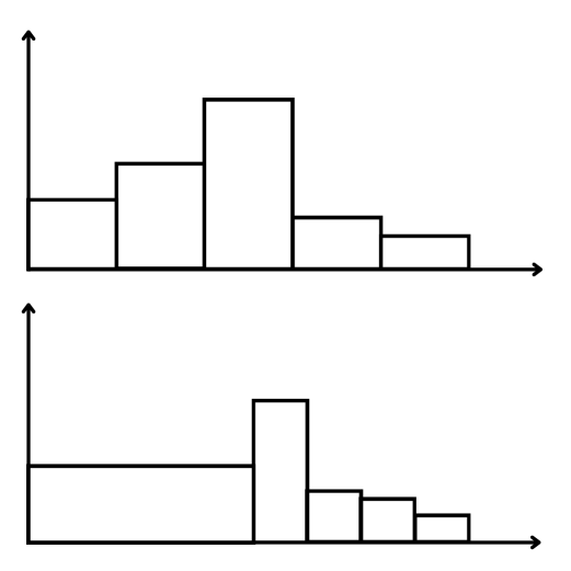
(a)

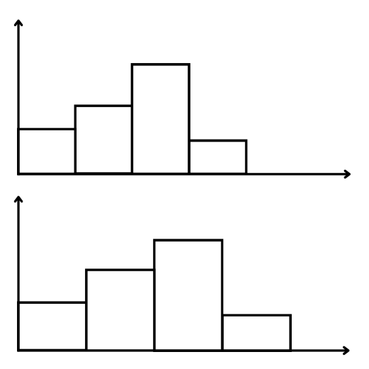
(b)

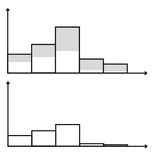
(c)

Figure 3. A visualization of our histogram maintenance strategy. (a) Extending the lowest bin as $R_{(k)}$ value grows. (b) Extending the range to contain unexpectedly large scores, and (c) subtracting a histogram (shaded) from another histogram.

(a) The lowest several bins of the histogram is consolidated into one, and the remaining bins are split into smaller bins. (b) The bins of a histogram are lengthened out to increase the maximum range of legal values. (c) The height of a histogram is decreased equal to the amount subtracted.

3.2.7. Summary and End-to-End Example

We now return to Example 1.1, and review the full practical workflow.

Example 3.1.

Alice hypothesizes that used cars that have similar feature values will have similar valuations. As such, she clusters listings based on their feature values using $k$-means clustering. She then builds a tree that groups close clusters into the same subtree. Then, she deploys the following algorithm.

1. It initializes an empty histogram for all nodes in the tree, including leaf clusters. It also initializes a priority queue that has a maximum capacity of at most $k$ elements. The queue will contain (score, element) tuples.

2. In each iteration, the algorithm chooses a leaf cluster by invoking the $\varepsilon$-greedy bandit algorithm on each layer of the tree index, which:

   1. With a decreasing probability, chooses a random child.

   2. Otherwise, chooses the child that greedily maximizes marginal gain in STK.

   3. This process repeats until it reaches a leaf cluster.

3. It takes a sample from the chosen leaf and computing the sample’s score.

4. It updates the histograms of the leaf node and all of its parent nodes in the tree. The histogram class adjusts its bin borders when $S_{(k)}$ becomes too large or if a score that exceeds its limit is sampled.

5. After an initial threshold, the algorithm periodically checks the failure conditions. It may fall back to a flat index or a uniform sample over the remaining elements.

6. When Alice is satisfied with the solution quality, she terminates and retrieves the elements in the priority queue.

4. Analysis

In this section, we establish a theoretical regret bound. Our main result (Theorem 4.4) states that Algorithm 1 finds a solution whose STK is lower bounded by $(1-\exp(-1-1/2T))\text{OPT}-O(T^{2/3})$ in expectation. That is, the quality of running solution approaches a constant factor of $1-1/e\approx 0.63$ with a multiplicative and an additive regret.

To show this, we will first assume that all $L$ distributions of arms are known. Under this assumption, we will reduce the problem of assigning budgets to each arm as a stochastic diminishing returns (DR) submodular maximization problem (§ 4.1). Intuitively, assigning a larger budget increases the expected quality of the solution, but larger budgets have diminishing returns. A simple greedy algorithm achieves $(1-1/e)$-approximation to the optimal in expectation (Asadpour and Nazerzadeh, 2016). Finally, we generalize the result to unknown distributions (§ 4.2). We show that our algorithm, with high probability, chooses a nearly optimal arm. We then apply this to a standard formula for analyzing submodular maximization algorithms.

4.1. Objective Function Analysis

In the classical MAB setting, the reward obtained from a distribution contributes directly to the overall objective. Thus, the greedy action is optimal. In Top-$K$ MAB, however, the greedy action may be suboptimal. Let there be distributions $D_{1}$ and $D_{2}$, where $D_{1}$ has a higher mean than $D_{2}$, but $D_{2}$ has a higher variance. Suppose we are about to make the first sample ($t=1$). If $T\gg k$, it may be optimal to sample from $D_{2}$, even though $D_{1}$ has a higher mean.

The main objective of this section is to establish that the value of a greedy action is within a constant factor to optimal. The key idea is that the STK objective exhibits a diminishing returns property. Specifically, it is monotone and DR-submodular (Soma and Yoshida, 2018) w.r.t. the sampling budget allocated to each cluster. Then, we reduce the top-$k$ sampling problem, under known distributions, as the stochastic monotone submodular maximization problem under matroid constraint, which is NP-hard but admits a $(1-1/e)$-approximate adaptive greedy algorithm (Asadpour and Nazerzadeh, 2016).

Preliminaries. Let us define the desirable properties. Let $S\in\mathcal{M}(\mathbb{Z})$ be a multiset of integers, and let $f:\mathcal{M}(\mathbb{Z})\to\mathbb{Z}^{+}$ be a function that returns a number given a multiset. An example of such function $f$ is the STK function (Equation 1). Let us denote the multiplicity of element $x$ in multiset $S$ as $m_{S}(x)$. Given two multisets $X,Y\in\mathcal{M}(\mathcal{X})$, we say that $X\leq Y$ when $m_{X}(x_{i})\leq m_{Y}(x_{i})$ for all $x_{i}\in\mathbb{Z}$. For example, $\{0,1\}\leq\{0,0,1,1,1\}$, but $\{0,0,1\}$ and $\{0,1,1\}$ are incomparable. The $\leq$ operator defines a lattice over multisets.

Then, $f$ is monotone iff

(4) $$f(X)\leq f(Y)\quad$$

for all $X,Y\in\mathcal{M}(\mathbb{Z})$ where $X\leq Y$.

Next, a function $f$ is DR-submodular over integer lattice iff

(5) $$f(X+x_{i})-f(X)\geq f(Y+x_{i})-f(Y)$$

for all $X,Y\in\mathcal{M}(\mathbb{Z})$ s.t. $X\leq Y$, and $x_{i}\in\mathbb{Z}$.

Analysis of STK function. With the definitions established, we now show that the STK objective function is monotone and DR-submodular. Intuitively, adding new elements to some set never decreases its STK. Furthermore, adding an element to a small set has potential to significantly improve its STK, whereas adding the same element to a larger set improves STK by a smaller amount.

Theorem 4.1.

$\text{STK}(S)$ is monotone and DR-submodular.

Proof.

Let $x\in\mathcal{X}$. Then,

(6) $$\text{STK}(S\cup\{x\})=\begin{cases}\text{STK}(S)+x-S_{(k)}&\text{if }x\geq S_{(k)}\\ \text{STK}(S)&\text{otherwise.}\end{cases}$$

Since adding an element to $S$ does not decrease STK, that is $\text{STK}(S\cup\{x\})\geq\text{STK}(S)$, the function $\text{STK}(S)$ is monotonic. Next, let $S_{1},S_{2}$ be multisets such that $S_{1}\leq S_{2}$. Then, we prove that

(7) $$\text{STK}(S_{1}\cup\{x\})-\text{STK}(S_{1})\geq\text{STK}(S_{2}\cup\{x\})-\text{STK}(S_{2}).$$

This is equivalent to the following.

(8) $$\mathbb{I}(x\geq{(S_{1})}_{(k)})(x-{(S_{1})}_{(k)})\geq\mathbb{I}(x\geq{(S_{2})}_{(k)})(x-{(S_{2})}_{(k)})$$

Clearly ${(S_{1})}_{(k)}\leq{(S_{2})}_{(k)}$ since $S_{1}\leq S_{2}$. Hence,

(9) $$x-{(S_{1})}_{(k)}\geq x-{(S_{2})}_{(k)}\geq 0.$$

By total ordering of $\mathbb{Z}$, either $x<{(S_{1})}_{(k)}$, ${(S_{1})}_{(k)}\leq x<{(S_{2})}_{(k)}$, or ${(S_{2})}_{(k)}\leq x$. Hence,

(10) $$\mathbb{I}(x\geq{(S_{1})}_{(k)})\geq\mathbb{I}(x\geq{(S_{2})}_{(k)})\geq 0.$$

By Equation 9 and Equation 10, Equation 8 always holds, proving DR-submodularity. ∎

Analysis of budget oracle. A budget restricts how many times we can sample from each arm or cluster. For example, suppose are just two clusters A and B that divide a dataset in half. A valid budget might be $\{(A,2),(B,10)\}$ which means to sample from A twice and sample from B 10 times. Assume $\text{BS}:(\mathbb{Z}^{+}_{0})^{L}\to\mathbb{R}$ is a function that evaluaes a budget allocation. It takes as input a mapping from each of the $L$ arms/clusters to a non-negative integer. Then, it returns the value of that budget. Let $X$ be a budget, and let $X_{l}$ be the budget allocated to $\mathcal{D}_{l}$. We define $S_{r}$ to be a random variable representing the outcome of the following procedure.

Procedure 4.1. Start with multiset $S=\emptyset$. Then, sample the $l$^th cluster $x_{l}$ times independently, for each $l\in[L]$. Add all scores to the running set of scores $S$ and return $S$. We define $\text{BS}(X)$ to be

(11) $$\text{BS}(X)=\mathbb{E}[\text{STK}(S_{r})].$$

Then, the following theorem holds.

Theorem 4.2.

$\text{BS}(X)$ is monotone and DR-submodular.

Intuitively, sampling more never hurts. Sampling one more time is highly beneficial if the existing budget is tight, and less beneficial if the existing budget is plentiful.

Proof.

Analogous to multisets, two integer vectors $X,Y$ satisfy $X\leq Y$ iff $x_{i}\leq y_{i}$ element-wise. Let $X,Y\in(\mathbb{Z}^{+})^{L}$ be budget allocations s.t. $X\leq Y$. For each $l$, suppose there is a pre-generated infinite tape of i.i.d. samples from $D_{l}$. Let there be two agents: The first reads the first $x_{l}$ elements from the $l$th tape for each $l\in[L]$, and the second reads the first $y_{l}$ instead. Then, regardless of the values realized on the tapes, we have $S_{X}\subseteq S_{Y}$. By monotonicity of STK (Theorem 4.1), $\text{STK}(S_{X})\leq\text{STK}(S_{Y})$. Since the inequality holds in all outcomes, regardless of the realizations on the tapes, we have

(12) $$\mathbb{E}[\text{STK}(S_{X})]\leq\mathbb{E}[\text{STK}(S_{Y})]$$

which proves the monotonicity of BS.

Next, let $X,Y\in(\mathbb{Z}^{+})^{L}$ such that $X\leq Y$, and let some $i\in[L]$. Then, we devise a similar experiment.

Procedure 4.2. For each $l\in[L]$, initialize an infinite tape of i.i.d. samples from the distribution $D_{l}$. Initialize multisets $S_{X^{\prime}},S_{X},S_{Y^{\prime}},S_{Y}$ as $\emptyset$. These multisets have budgets $X+\chi_{i},X,Y+\chi_{i}$, and $Y$, respectively. Consider one multiset and its corresponding budget vector $Z$. Then, add the first $z_{l}$ elements of the $l$th infinite tape for all $l\in[L]$. Repeat for each of the four multisets.

By construction of Procedure 4.1, we have $S_{X^{\prime}}\geq S_{X}$, $X_{Y^{\prime}}\geq S_{Y}$, and $S_{Y}\geq S_{X}$. By DR-submodularity of STK (Theorem 4.1),

(13) $$\text{STK}(S_{X^{\prime}})-\text{STK}(S_{X})\geq\text{STK}(S_{Y^{\prime}})-\text{STK}(S_{Y}).$$

Since this holds in every possible outcome,

(14) $$\mathbb{E}[\text{STK}(S_{X^{\prime}})-\text{STK}(S_{X})]\geq\mathbb{E}[\text{STK}(S_{Y^{\prime}})-\text{STK}(S_{Y})].$$

By linearity of expectation,

(15) $$\mathbb{E}[\text{STK}(S_{X^{\prime}})]-\mathbb{E}[\text{STK}(S_{X})]\geq\mathbb{E}[\text{STK}(S_{Y^{\prime}})]-\mathbb{E}[\text{STK}(S_{Y})].$$

By construction of Procedure 4.1,

(16) $$\mathbb{E}[\text{STK}(S_{X^{\prime}})]=\text{BS}(X+\chi_{i}),\quad\mathbb{E}[\text{STK}(S_{X})]=\text{BS}(X),$$

(17) $$\mathbb{E}[\text{STK}(S_{Y^{\prime}})]=\text{BS}(Y+\chi_{i}),\quad\mathbb{E}[\text{STK}(S_{Y})]=\text{BS}(Y).$$

By substitution,

(18) $$\text{BS}(X+\chi_{i})-\text{BS}(X)\geq\text{BS}(Y+\chi_{i})-\text{BS}(Y)$$

which proves DR-submodularity of BS. ∎

Our final task is establishing $(1-1/e)$-approximation of the adaptive greedy procedure.

Remark 0.

The top-$k$ bandit problem with known distributions reduces to a monotone submodular maximization problem under uniform matroid constraint.

We let the objective function be $\text{BS}(X)$ defined in Equation 11, which we proved to be monotone and submodular (Theorem 4.1). The cardinality constraint $T$ is a uniform matroid. Hence, maximizing $\text{BS}(S)$ under uniform matroid constraint also maximizes the top-$K$ bandit with known distributions.

Corollary 4.3.

Adaptive greedy, which chooses distribution that greedily maximizes marginal gain of $\text{STK}(S)$ in each iteration, achieves $(1-1/e)$-approximation to the optimal adaptive algorithm.

Corollary 4.3 holds as a direct application of Theorem 4 in (Asadpour and Nazerzadeh, 2016).

4.2. Regret Analysis

Corollary 4.3 in § 4.1 establishes that, if distribution of all arms are known, then the adaptive greedy procedure achieves constant approximation. Of course, we cannot assume that the distributions are known. In this section, we show the following theorem.

Theorem 4.4.

The expectation of STK by Algorithm 1 at iteration limit $T$ is lower bounded by $\left(1-e^{-1-\frac{1}{2T}}\right)\text{OPT}-\tilde{O}\left(T^{2/3}\right)$ if there is a finite collection of arms and the scoring domain is a finite set of non-negative integers.

Our proof strategy combines standard $\varepsilon$-greedy bandit analysis technique with the proof of Theorem 4 in (Asadpour and Nazerzadeh, 2016). We divide all outcomes into the clean event and the dirty event. In the clean event, the algorithm estimates all bin values to high precision. The dirty event is the complement of the clean event. Since the dirty event occurs with low probability, the algorithm closes the gap between $\mathrm{OPT}$ and $\text{STK}(S_{t})$ by a factor of $\left(\frac{1}{T}-\tilde{O}\left(T^{-1/3}\right)\right)$ due to monotone submodularity.

Proof.

The exploration rate for Algorithm 1 at iteration $t$ is given by $\varepsilon_{t}=t^{-1/3}$. Then by integration, the total expected number of exploration rounds by iteration $T$ is $t^{2/3}$. Let $X_{t}$ be the number of exploration rounds by iteration $t$, and let $X_{t}^{l}$ be the number of explorations on arm $D_{l}$ by iteration $t$. By the repeated applications of the Hoeffding bound, the following statements hold.

The total number of exploration rounds is close to expected with high probability.

(19) $$P\left[\left|X_{t}-\mathbb{E}[X_{t}]\right|\leq\tilde{O}\left(t^{-1/3}\right)\right]\leq 1-t^{-2}$$

A similar bound holds for the number of exploration rounds per arm. We are multiplying the probability $1+L$ times to ensure that the total exploration rounds are close to expectation and that all $L$ arms’ exploration rounds are close to expectation.

(20) $$P\left[\left|X_{t}^{l}-\mathbb{E}[X_{t}^{l}]\right|\leq\tilde{O}\left(t^{-1/3}\right)\;\forall l\right]\leq{\left(1-t^{-2}\right)}^{1+L}$$

Similarly, we upper bound the probability that the empirical probability estimate for each outcome $x_{i}$ for each arm is inaccurate compared to the ground truth. We denote all empirical estimates with an overline. This time, multiply the RHS an additional $LB$ times to ensure the bound holds for each arm-outcome pair.

(21) $$P\left[\left|\overline{P}[X_{l}=x_{i}]-P[X_{l}=x_{i}]\right|\leq\tilde{O}\left(t^{-1/3}\right)\;\forall l\;\forall b\right]\leq{\left(1-t^{-2}\right)}^{1+L+LB}$$

In Equation 21, $X_{l}$ is the random variable representing a sample from $D_{l}$, $P[X_{l}=x_{i}]$ is the probability that $X_{l}$ is a particular outcome $x_{i}$, and $\overline{P}[X_{l}=x_{i}]$ is the estimate of the probability using samples. Note that RHS of Equation 21 is equivalent to $1-\tilde{O}\left(t^{-2}\right)$.

If Equation 21 holds, then clearly

(22) $$\left|\overline{\mathbb{E}[\Delta_{t,l}]}(S_{t-1})-\mathbb{E}[\Delta_{t,l}](S_{t-1})\right|\leq\tilde{O}\left(t^{-1/3}\right).$$

where $\mathbb{E}[\Delta_{t,l}]$ is the expected marginal gain in STK for sampling from $D_{l}$ and $S_{t-1}$ is the set obtained by the greedy procedure up to the previous iteration.

A standard result in the known distribution, adaptive setting is

(23) $$\mathbb{E}[\Delta_{t}]\geq\frac{1}{T}(\mathrm{OPT}-\text{STK}(S_{t}))$$

where $\mathrm{OPT}$ is the expected score of the optimal algorithm (Asadpour and Nazerzadeh, 2016). In the top-$k$ bandit setting, by Equation 21 and 22,

(24) $$\mathbb{E}[\Delta_{t+1}]\geq\left(1-O\left(t^{-2}\right)\right)\cdot\left(\frac{1}{T}(\mathrm{OPT}-\text{STK}(S_{t}))-\tilde{O}\left(t^{-1/3}\right)\right)$$

since with probability at least $1-O\left(t^{-2}\right)$, Algorithm 1 chooses an arm with marginal gain at most $\tilde{O}\left(t^{-1/3}\right)$ smaller than the arm chosen by adaptive greedy with known distributions.

Then, by algebraic simplification,

(25) $$\mathbb{E}[\Delta_{t+1}] \geq\frac{1}{T}(\text{OPT}-\text{STK}(S_{t}))\left(1-O\left(t^{-2}\right)\right)-\tilde{O}\left(t^{-1/3}\right).$$

Next, let $\delta_{t}=\text{OPT}-\text{STK}(S_{t})$. Then since

(26) $$\delta_{t+1}=\delta_{t}-\mathbb{E}[\Delta_{t+1}],$$

by substitution,

(27) $$\delta_{t}-\delta_{t+1}\geq\frac{1}{T}\delta_{t}\left(1-O\left(t^{-2}\right)\right)-O\left(t^{-1/3}\right)$$

which implies

(28) $$\delta_{t+1}\leq\delta_{t}\left(1-\frac{1}{T}+\frac{1}{T}O\left(t^{-2}\right)\right)+\tilde{O}\left(t^{-1/3}\right).$$

This gives us a recurrence relation for $\delta_{t}$ to upper bound it. For simplicity, let

(29) $$a_{t}=1-\frac{1}{T}+\frac{1}{T}O(t^{-2}),$$

Then by a standard application of the homogeneous recurrence relations formula, we have

(30) $$\delta_{T}=\left(\prod_{t=0}^{T-1}a_{t}\right)\left(\text{OPT}+\sum_{i=0}^{T-1}\frac{O\left(i^{-1/3}\right)}{\prod_{j=0}^{i}a_{j}}\right).$$

We wish to upper bound $\delta_{T}$, which means upper and lower bounding $\prod_{j=1}^{i}a_{j}$. We know $a_{j}$ is bounded by

(31) $$1-\frac{1}{T}\leq a_{j}\leq 1-\frac{1}{T}+\frac{O(1)}{T}.$$

Then, by substitution,

(32) $$\left(1-\frac{1}{T}\right)^{T}\leq\prod_{j=1}^{i}a_{j}\leq\left(1-\frac{1}{T}+\frac{O(1)}{T}\right)^{T}.$$

(33) $$\exp\left(T\log\left(1-\frac{1}{T}\right)\right)\leq\prod_{j=0}^{i}a_{j}\leq\exp\left(T\log\left(1-\frac{1}{T}+\frac{O(1)}{T}\right)\right)$$

By Taylor expansion of the log terms and simplification, we obtain

(34) $$e^{-1-\frac{1}{2i}}\leq\prod_{t=0}^{i}a_{j}\leq e^{-1+O(1)}.$$

Substituting back into Equation 30, we get

(35) $$\delta_{T}\leq e^{-1-\frac{1}{2T}}\left(\text{OPT}+\sum_{m=0}^{T-1}\tilde{O}\left(m^{-1/3}\right)e^{1+\frac{1}{2m}}\right).$$

Since $e^{1+\frac{1}{2m}}\leq O(1)$,

(36) $$\tilde{O}\left(m^{-1/3}\right)O(1)\leq\tilde{O}\left(m^{-1/3}\right)$$

so by integration,

(37) $$\delta_{T} \leq e^{-1-\frac{1}{2T}}\left(\text{OPT}+\tilde{O}\left(T^{2/3}\right)\right).$$

Now, since $\delta_{T}=\text{OPT}-\text{STK}(S_{T})$, by substitution and rearranging,

(38) $$\mathbb{E}[\text{STK}(S_{T})]\geq\left(1-e^{-1-\frac{1}{2T}}\right)\text{OPT}-\tilde{O}\left(T^{2/3}\right).$$

∎

Notice that as $T\to\infty$, we get

(39) $$\lim_{T\to\infty}e^{-1-\frac{1}{2T}}=e^{-1}$$

Hence, for large $T$, the lower bound is approximately $(1-1/e)\text{OPT}-O(T^{2/3})$. Intuitively, this happens when the greedy rounds become indistinguishable as that of the known distribution setting, with an unavoidable $O(T^{2/3})$ regret incurred from exploration rounds. If this holds, then the algorithm approaches 63% of the optimal.

5. Experiments

In this section, we conduct extensive experiments to demonstrate the efficacy of our solution. We answer the following questions.

1. How does Ours perform for intrinsic and extrinsic quality metrics at different time steps?

2. To what extent are the fallback strategies and histogram maintenance strategies described in § 3 effective?

3. How efficient is Ours compared to simpler baselines?

4. How well does Ours generalize to different types of data, such as tabular and multimedia data?

5. How well does Ours generalize to different types of scoring functions, such as regression and fuzzy classification models?

5.1. Preliminaries

Throughout this section, we report sum-of-top-$k$ (STK) as the target intrinsic objective, and Precision@K as the target extrinsic objective. Note that Recall@K is identical to Precision@K as the ground truth solution has $k$ elements. We also host high-resolution plots with additional metrics and configurations in our source code repository.

5.1.1. Algorithms

We implement the following algorithms in our standalone system. All algorithms sample without replacement.

1. Ours: Algorithm 1 combined with the index of § 3.2.2. We use $B=8$, $\alpha=0.1$, $\beta=1.1$, and $F=0.01$ by default.

2. UCB: A standard upper confidence bound (UCB) bandit algorithm combined with the index of § 3.2.2. We set the exploration parameter as 1.0 and initialize the mean using query-specific prior knowledge.

3. ExplorationOnly: A bandit which chooses a uniformly random non-empty child in each layer of the index of § 3.2.2.

4. UniformSample: Uniform sampling over the entire search domain, implemented via pre-shuffling of the data, then performing a sequential scan. UniformSample represents the average case result of Scan, as there is no additional run-time overhead.

5. ScanBest, ScanWorst: Scan over the domain where the elements are sorted in the best-case or worst-case order. This is meant to demonstrate theoretical limits.

6. SortedScan: Scan over an in-memory sorted index built on a new column that contains pre-computed UDF function values. SortedScan skips scoring function evaluation and priority queue maintenance.

5.1.2. Datasets

1. Synthetic data: We randomly generate $L$ normal distributions with $\mu\in[0,20]$ and $\sigma\in(0,5]$. We then draw a fixed number of samples from each distribution, which then serves as the leaf clusters of the index. We build the dendrogram over the means of each cluster. There are 20 clusters and 2,500 samples per cluster.

2. Tabular data: We use the US Used Cars dataset (Mital, [n. d.]), collected from an online reseller (CarGurus, [n. d.]). We clean the data by projecting boolean and numeric columns, turning each column numeric, imputing missing values with column mean, then normalizing input features. The cleaned dataset has 11 columns: three boolean columns (frame damaged, has accidents, is new), six numeric columns (daysonmarket, height, horsepower, length, mileage, seller rating), one target column (price), and one key column (listing id). The target feature (price) is used for model training but excluded from indexing and querying. We build an index over a subset of $100,000$ rows with 500 leaf clusters.

3. Multimedia data: We use the ImageNet (Deng et al., 2009) dataset. We build the index and perform queries over a random subset of $320,000$ images. We scale each image to a 16x16x3 tensor, including the color channels, and flatten it to a vector. We then apply $k$-means clustering over a subsample of 100,000 images with 25 clusters. Finally, we assign all images to their closest cluster and build a dendrogram.

5.1.3. Scoring Functions

1. Synthetic data: The scoring function for synthetic data is the simple ReLU function, $f(x)=\max(0,x)$, to ensure non-negativity.

2. Tabular data: We train a regression model to predict a listing’s price, using XGBoost (Chen and Guestrin, 2016) with default parameters, on a subset of 1 million rows. The train split is disjoint from the split used for indexing and query evaluation. We use a batch size of 1 on CPU for inference.

3. Multimedia data: We use a pre-trained ResNeXT-64 model’s softmax layer to obtain its confidence that an image belongs to a particular label. Three target labels were chosen randomly. We use a batch size of 400 on GPU for inference.

5.1.4. Hardware Details

We ran all experiments on a dedicated server with a 13th Gen Intel i5-13500 (20 cores @ 4.8GHz) CPU, an NVIDIA RTX™ 4000 SFF Ada Generation GPU, and 64GB RAM running Ubuntu 22.04.

5.2. Synthetic Data

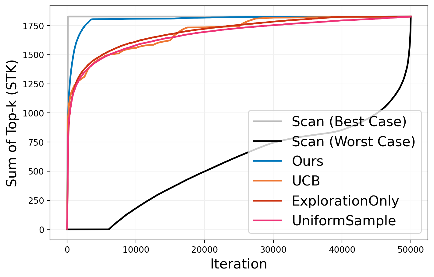
(a) STK

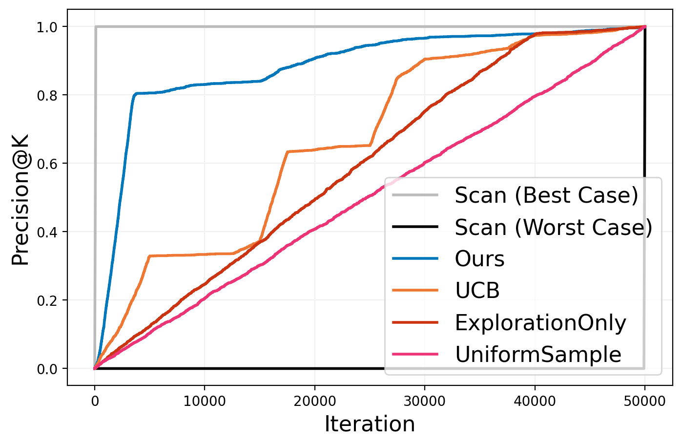
(b) Precision@K

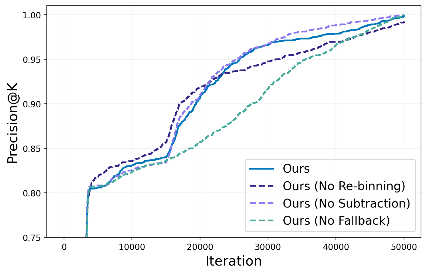
(c) Ablation study

Figure 4. Selecting $100$ highest numbers from synthetic normally distributed data ($n=50,000$) with 20 clusters. Averaged over 25 runs. (a-b) STK, Precision@K vs time. (c) Ablation study. Note the $y$-axis cutoff.

We run our algorithm and baseline algorithms on synthetic data, with $k=100$ and $T=50,000$. We also conduct an ablation study. We do not report latency for this dataset, since the number of iterations is an indicator of latency for synthetic data.

Figure 4 shows the result of this experiment. There are three main takeaways. First, Ours out-performs baseline algorithms in terms of both STK (Figure 4a) and Precision@K (Figure 4b). Ours reaches near-optimal STK rapidly. However, near-optimal Precision@K requires a much larger number of iterations. Second, the curve for UCB is piecewise-continuous, since it chooses sub-optimal intermediate nodes after a good child is exhausted. Third, turning off various features does not significantly impact performance. That said, turning off fallback has the most negative impact.

5.3. Tabular Regression

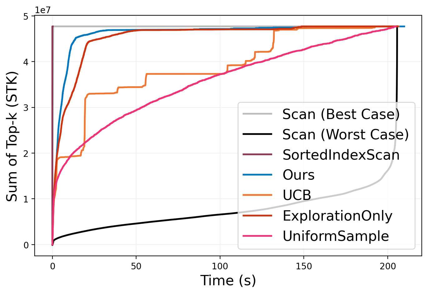
(a) STK

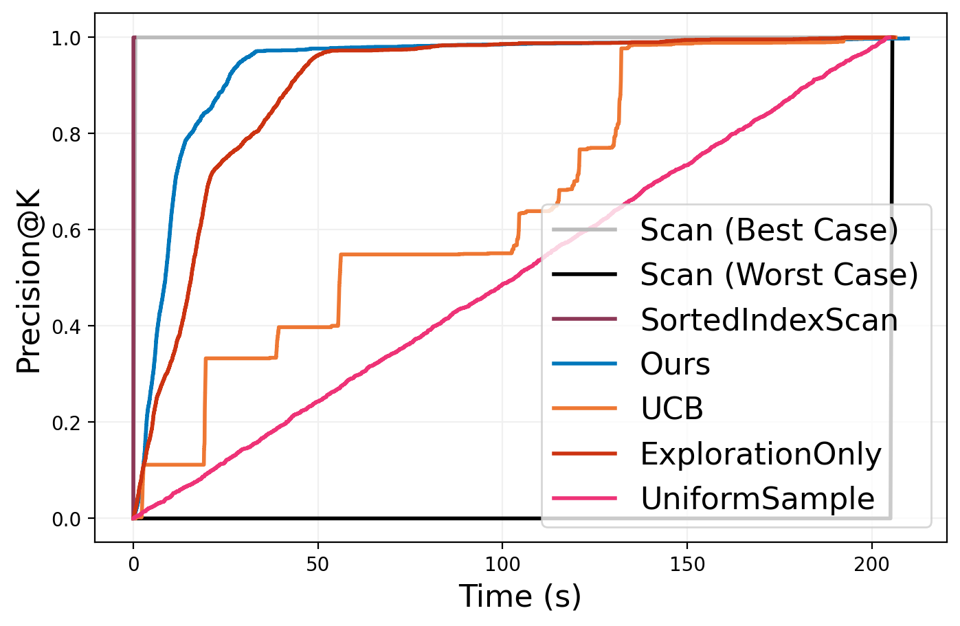
(b) Precision@K

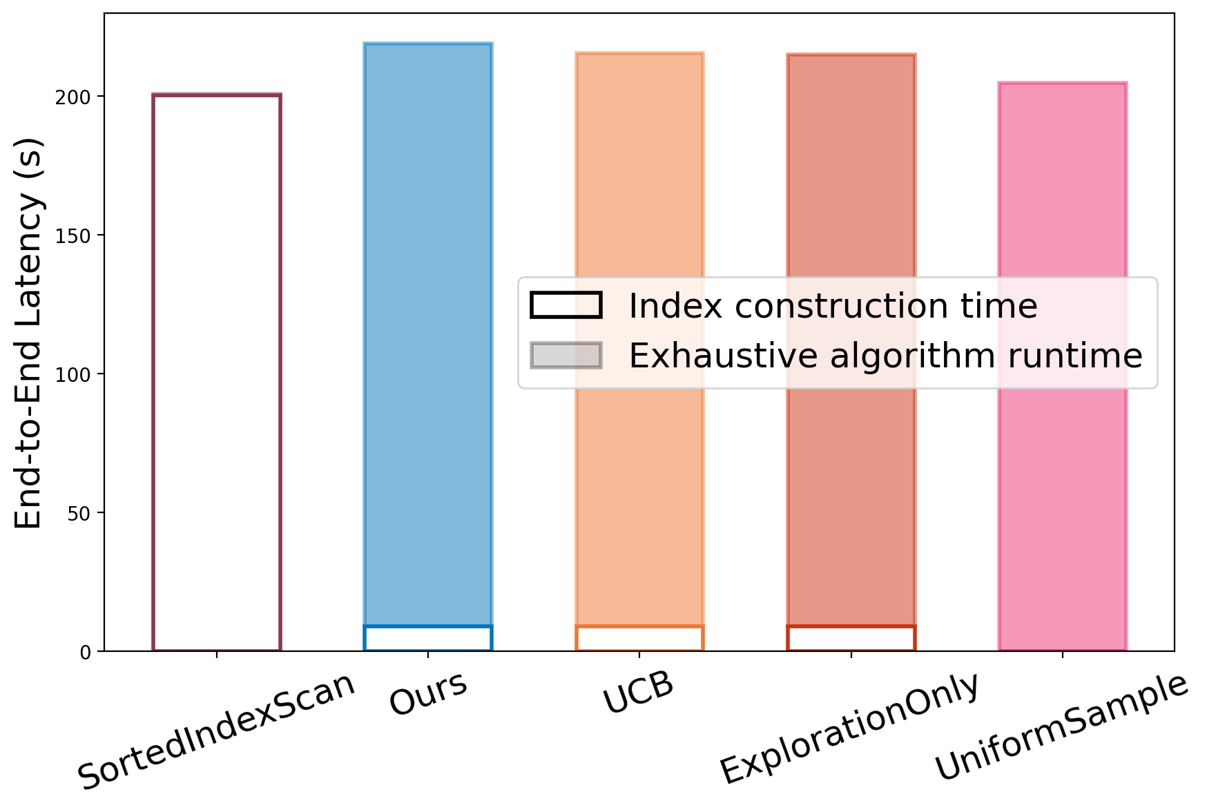
(c) End-to-end latency

Figure 5. Selecting 250 highest valued car listings form the UsedCars dataset ($n=100,000$) where the valuation is given by an XGBoost model. Averaged over 10 runs. (a-b) STK, Precision@K vs time. (c) End-to-end latency, which includes the index building time and the time to run the algorithm exhaustively over the entire dataset.

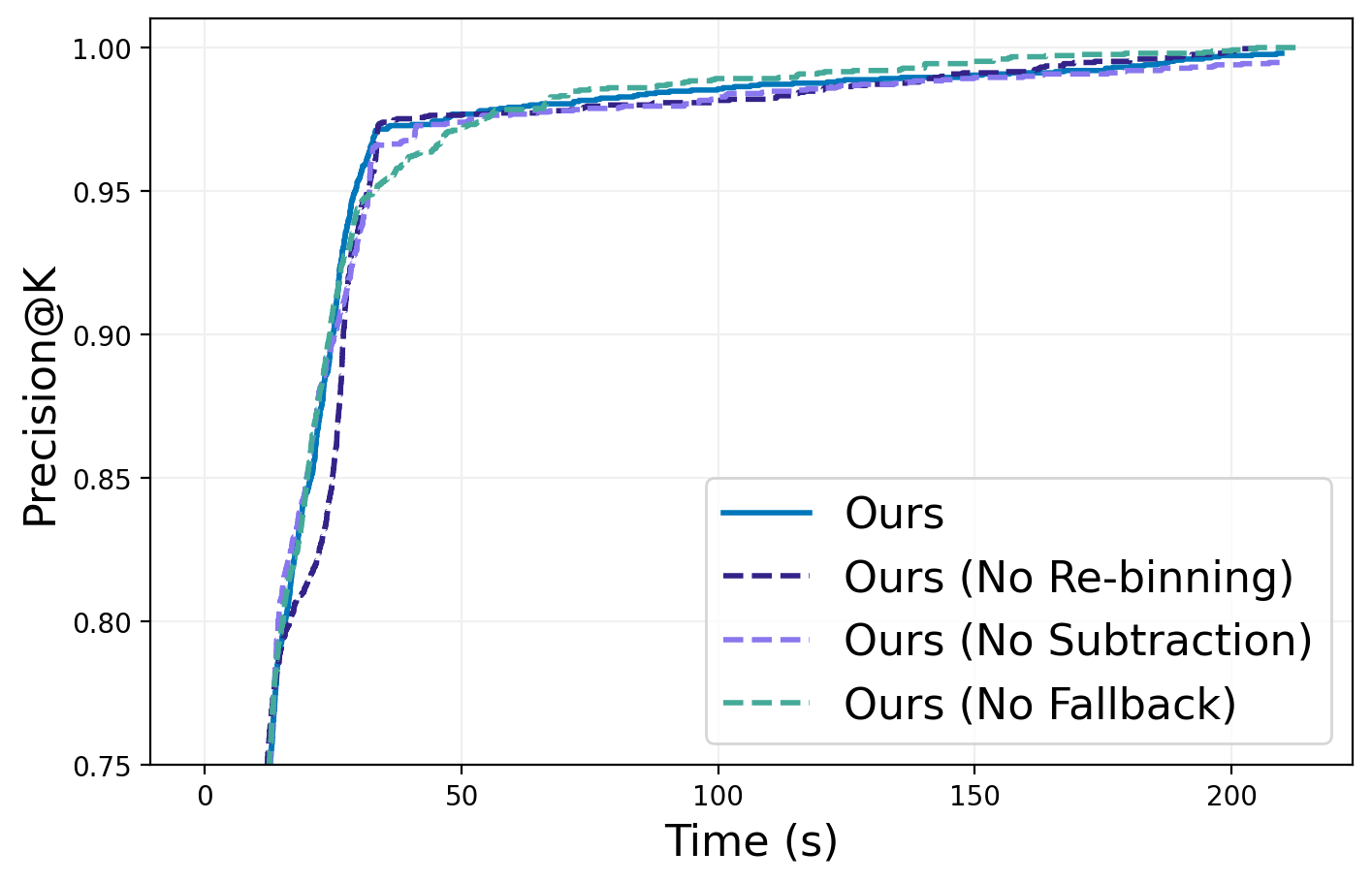
(a) Ablation study

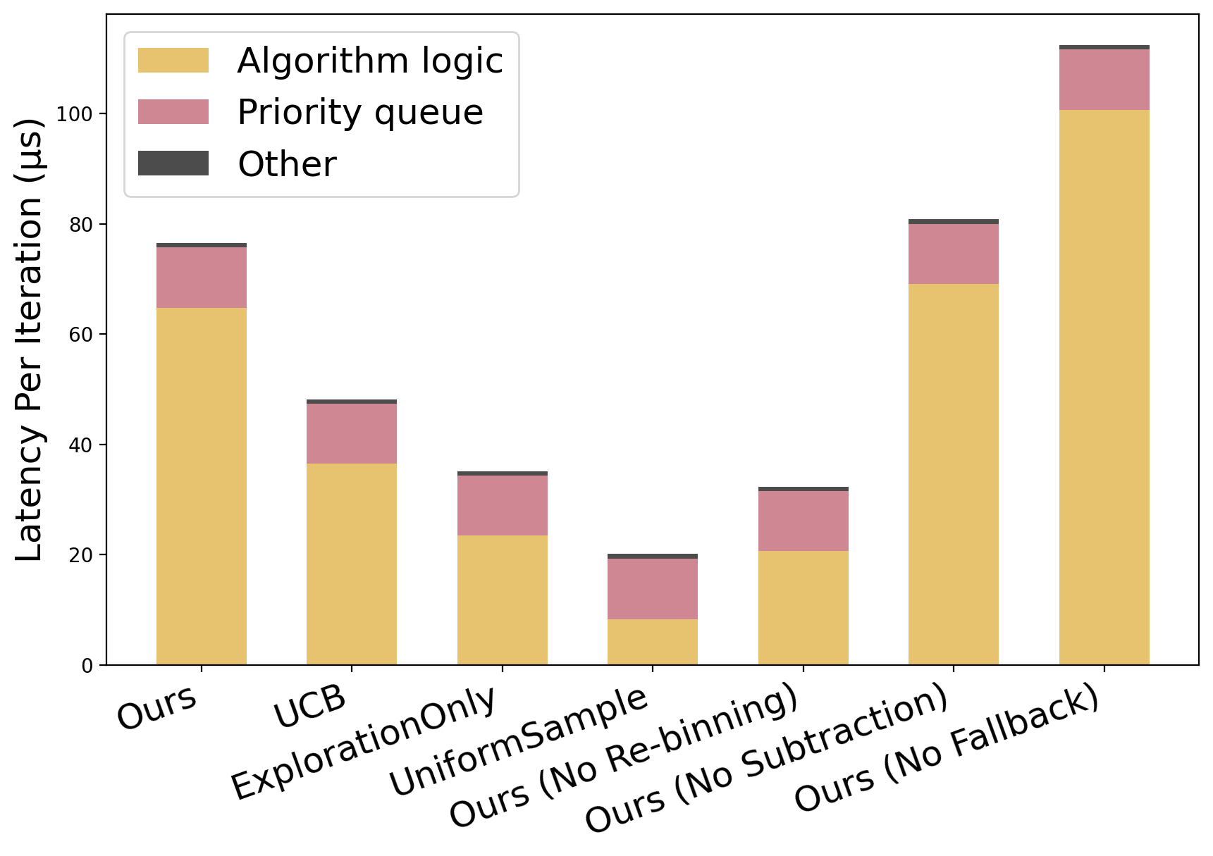
(b) Overhead per iteration

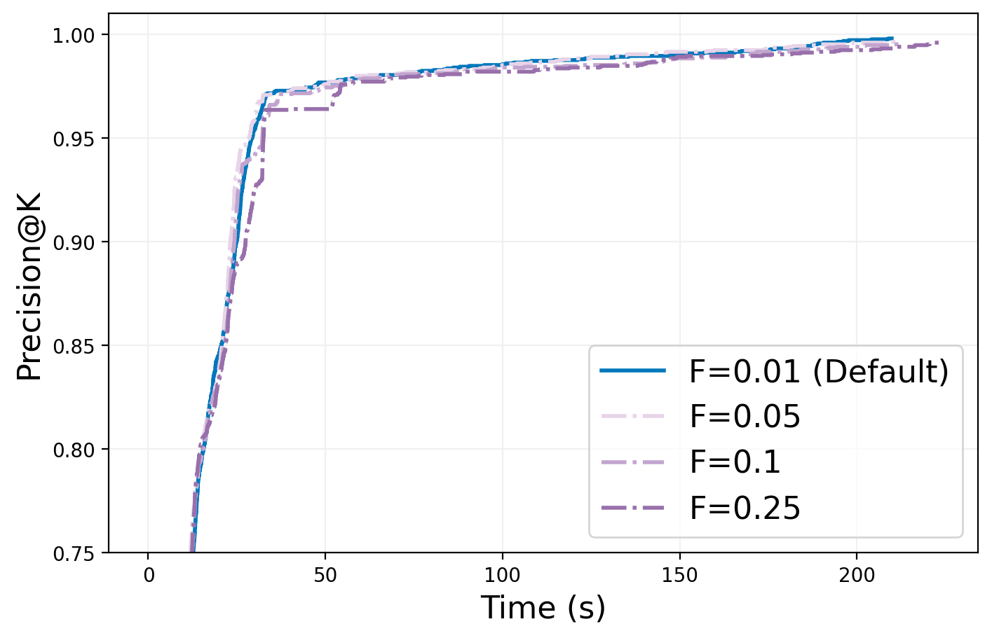
(c) Parameter study

Figure 6. Additional UsedCars results. (a) Ablation study. Note the $y$-axis cutoff. (b) Overhead incurred by different algorithms per iteration. Excludes scoring function latency (2ms/iter). (c) Parameter study. Variants have different fallback condition checking frequencies ($F$). Note the $y$-axis cutoff.

To test the applicability of Ours on tabular regression, we evaluate the algorithms on the task of selecting cars with the highest predicted valuation. This task also demonstrates the flexibility of the histogram re-binning strategy, as the maximum predicted price is unknown and unbounded. We set $k=250$ and $T=100,000$. We also report a SortedScan baseline, end-to-end and per-iteration latency analysis, and an ablation study.

Comparison to SortedScan. As shown in Figure 5a and 5b, SortedScan is very fast in query time, since it skips scoring function evaluation. However, as we observe in Figure 5c, SortedScan has a much higher index construction time than Ours. If the user only needs an approximate result, then Ours is much faster.

Comparison to other baselines. Figure 5a and 5b show the quality of results for Ours and all baselines. Ours significantly out-performs baselines and obtains near-optimal STK and Precision@K in a small number of iterations, as it identifies a few clusters that contain most of the exact solution. ExplorationOnly performs well, sometimes eclipsing Ours. We believe this is caused by two reasons. A few shallow leaf nodes that contain a large proportion of the ground truth solution, which ExplorationOnly is skewed towards. Furthermore, if the uniform value assumption does not hold, then Ours can fail to model the exact distributions. UCB significantly under-performs. Most likely, maximizing expected reward in each iteration causes UCB to select arms with high mean and low variance, which does not improve the running solution.

Parameter and Ablation Study. Figure 6a shows the result of an ablation study. All variants perform similarly, though with minor performance degradations if some features are turned off. Figure 6c shows a comparison of different fallback frequencies. Reducing the frequency slightly diminishes performance, but has minor impact.

Figure 6b shows the overhead of different algorithms. While Ours has high overhead, scoring function latency (2ms) is 18-25x longer. While enabling fallback incurs additional costs, it reduces average overhead over the entire query. Skipping re-binning decreases overhead, whereas skipping subtraction has little effect.

5.4. Image Fuzzy Classification

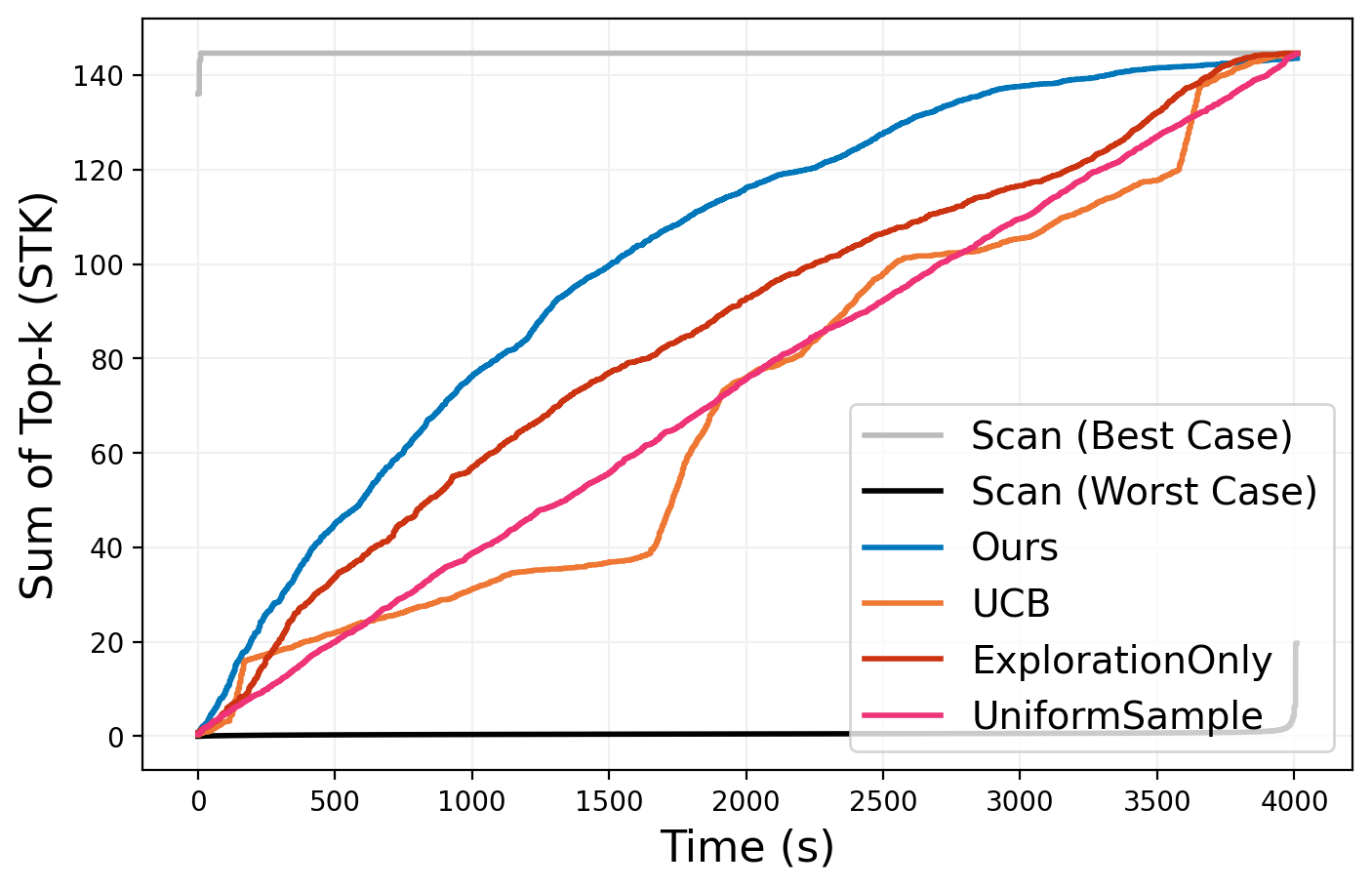
(a) Beacon, lighthouse (STK)

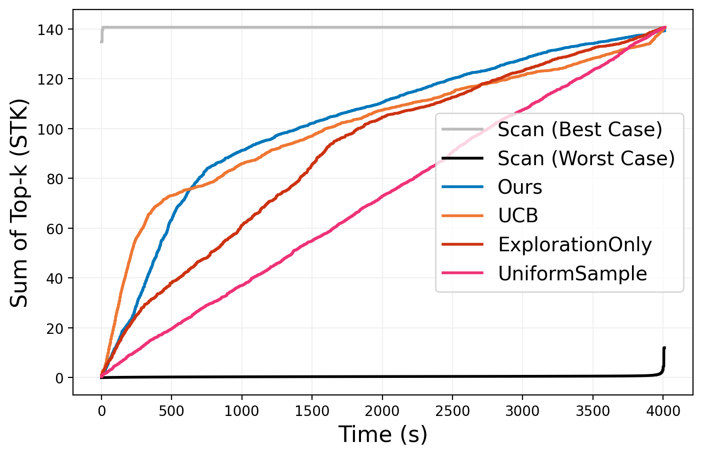
(b) Hand-held computer (STK)

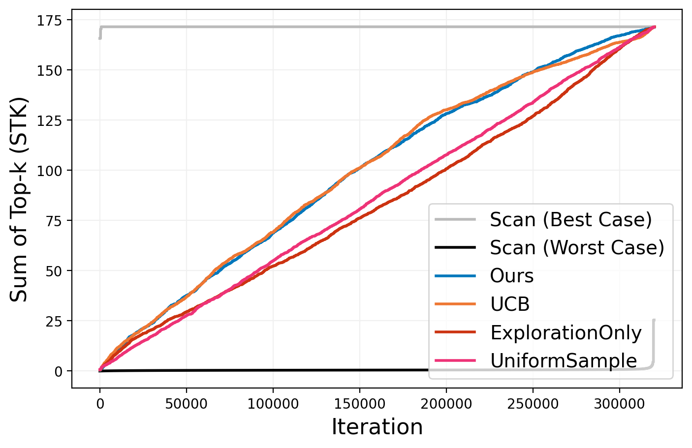
(c) Washing machine (STK)

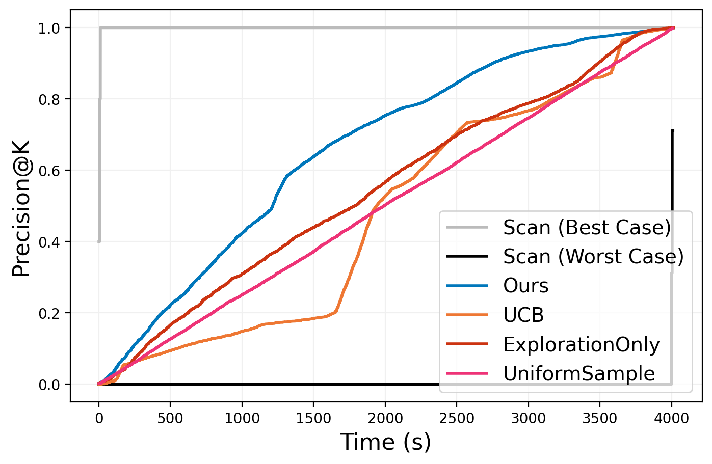
(d) Beacon, lighthouse (Precision@K)

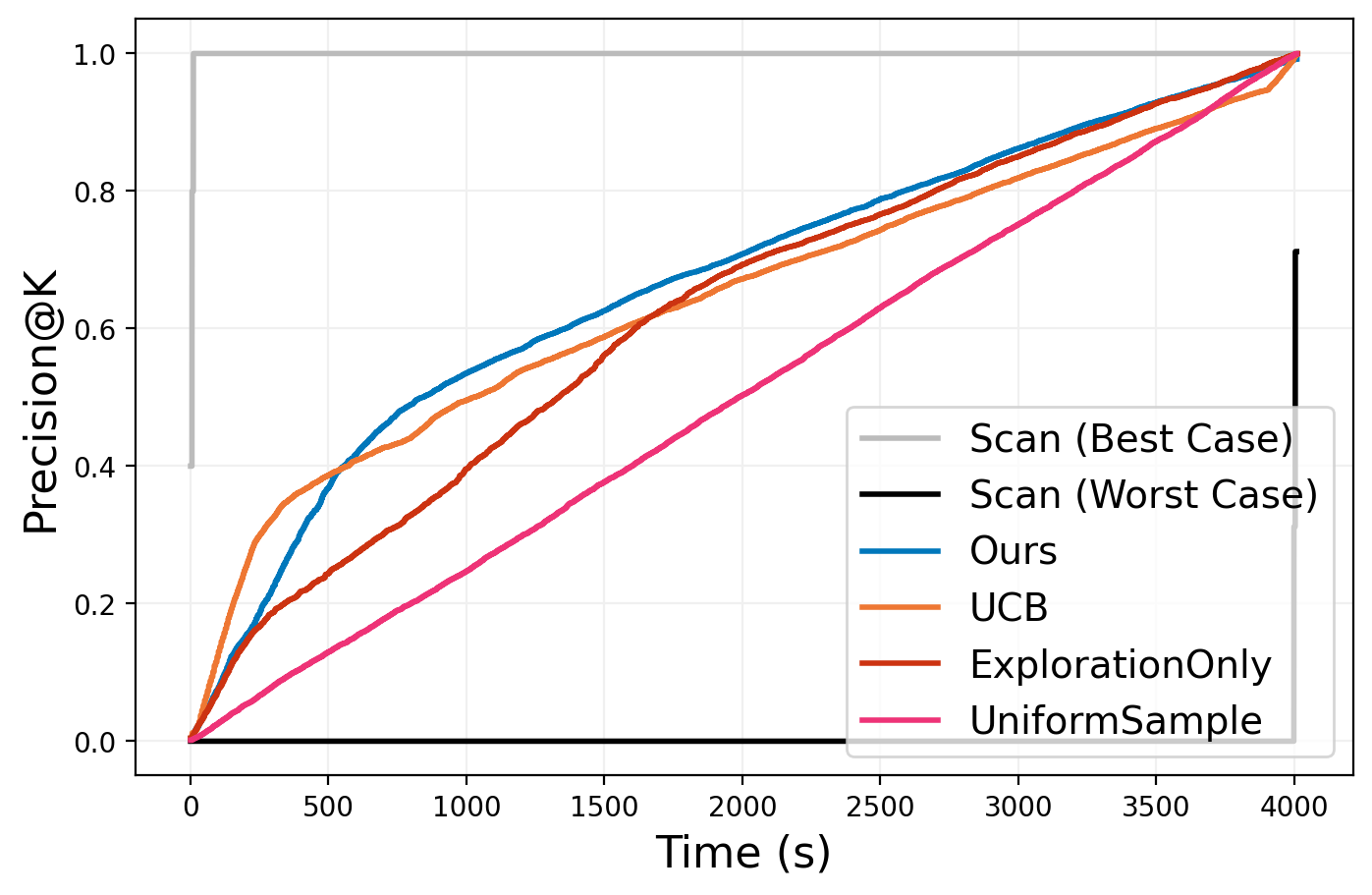
(e) Hand-held computer (Precision@K)

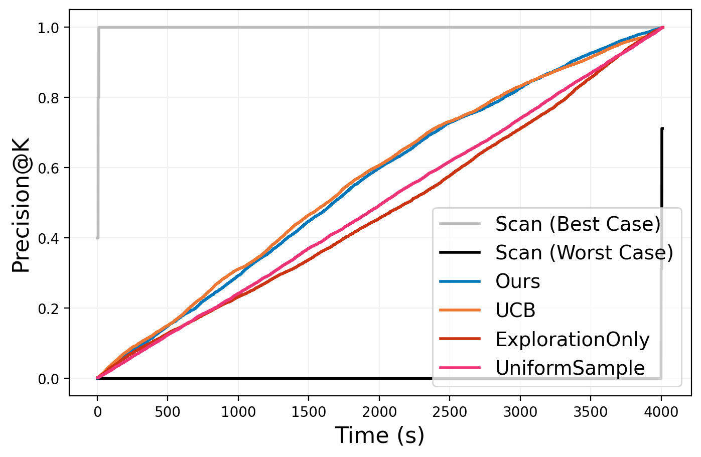
(f) Washing machine (Precision@K)

Figure 7. Selecting top 1000 images most confidently classified as a class label by a pre-trained ResNeXT model, over a subset of ImageNet ($n=320,000$). Averaged over 10 runs. (a-c) STK vs time. (d-f) Precision@K vs time.

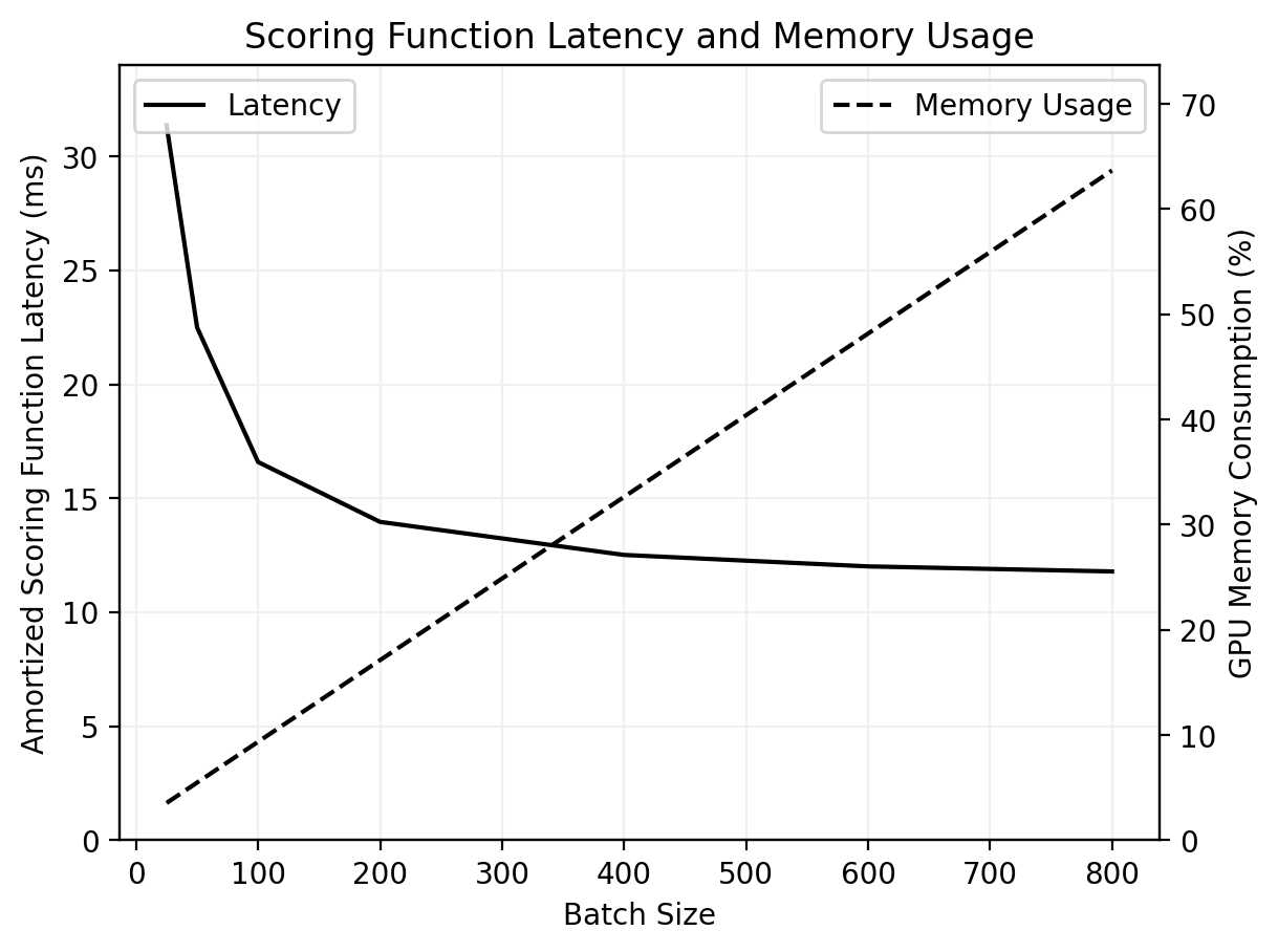
(a) Batch size vs. latency, memory

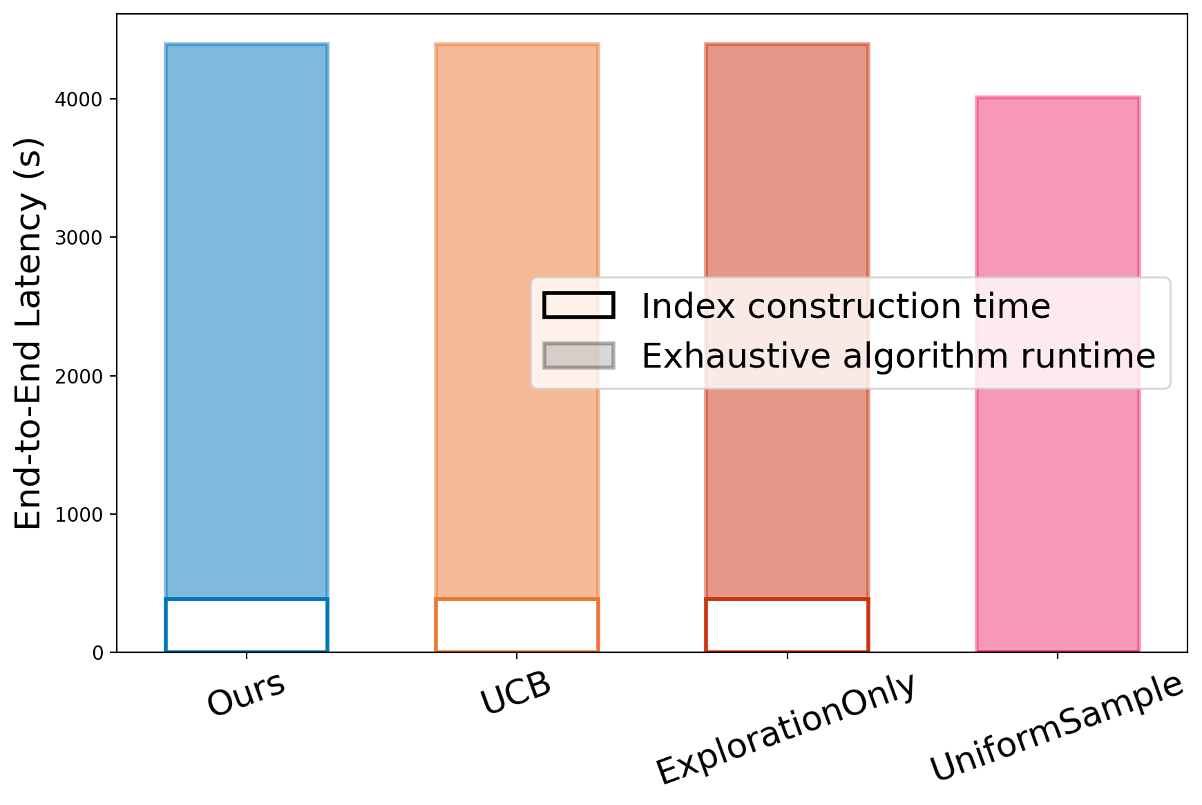
(b) End-to-end latency

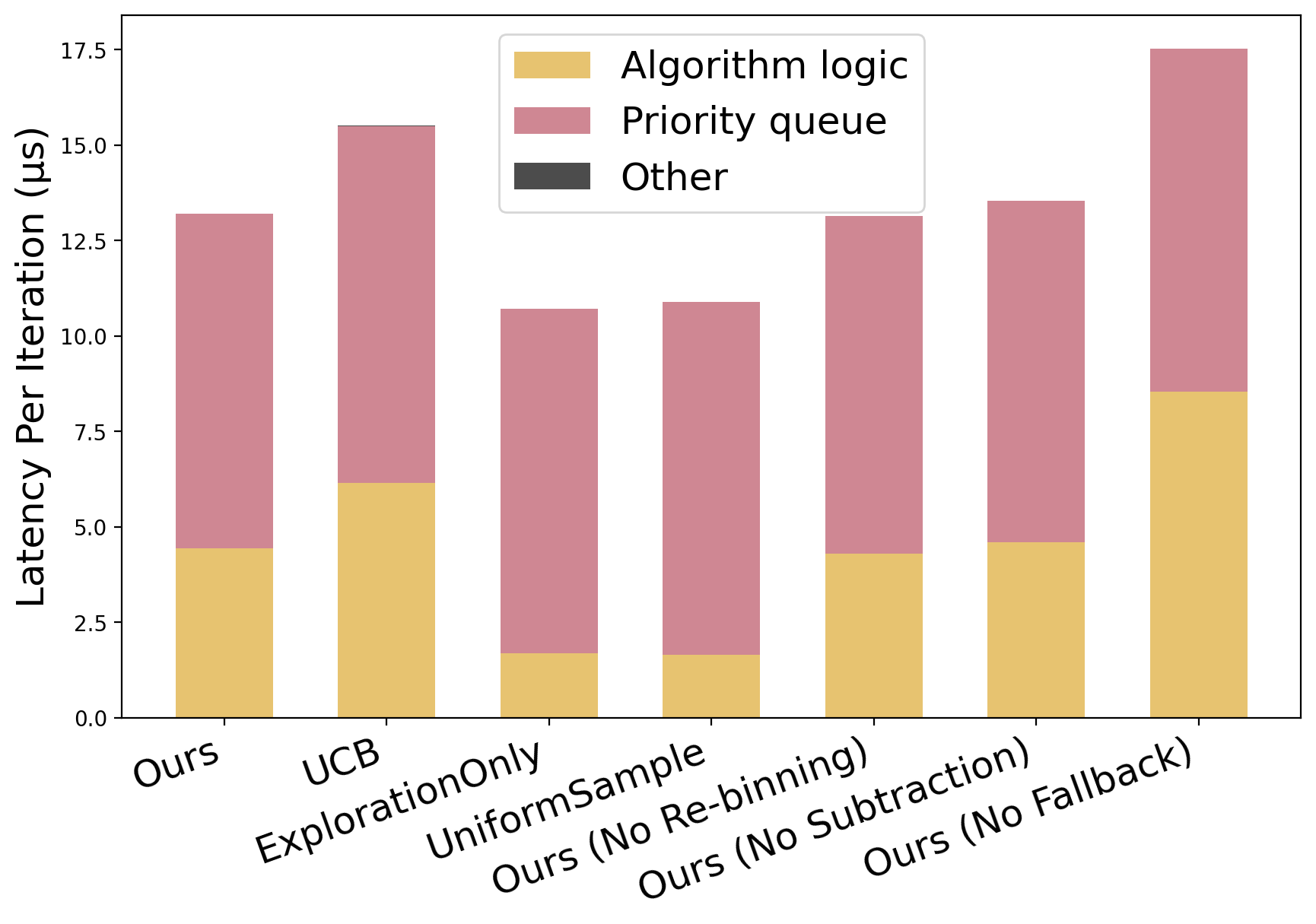
(c) Overhead per iteration

Figure 8. ImageNet latency results. (a) Scoring function latency, GPU memory consumption vs batch size. (b) End-to-end latency, which includes index buliding time and the time to run the algorithm exhaustively over the entire dataset. (c) Overhead incurred by different algorithms and ablation variants per iteration. Excludes scoring function latency (13ms/iter).

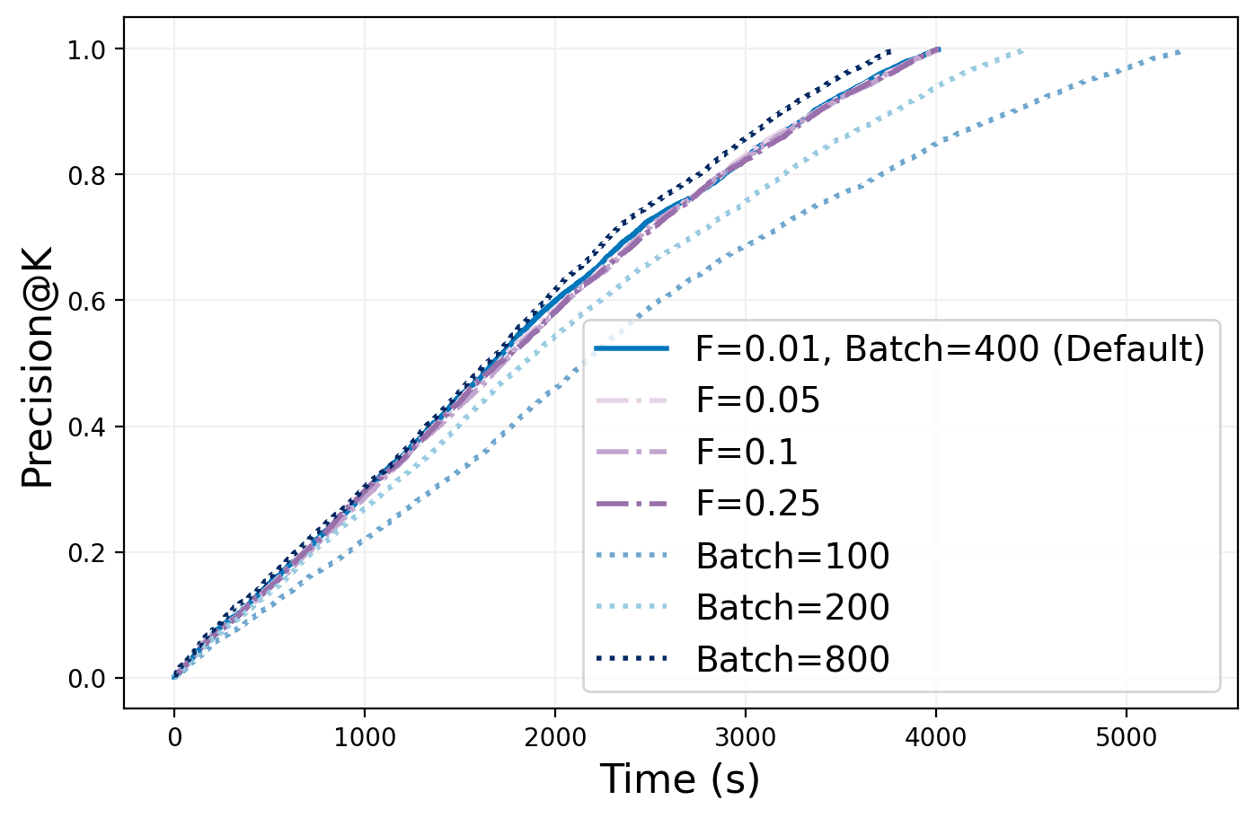
(a) Parameter study (beacon, lighthouse)

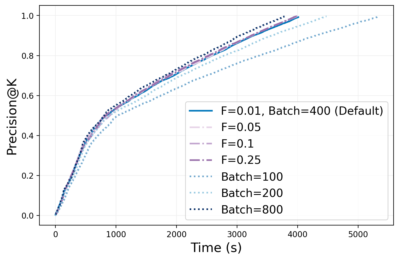
(b) Parameter study (hand-held computer)

(c) Parameter study (washing machine)

Figure 9. ImageNet parameter study. Variants have different fallback condition checking frequency ($F$) and batch sizes.

We evaluate algorithms for selecting images most confidently classified as some label. This task generalizes the binary classification task in He et al. (He et al., 2020) to fuzzy classification. We let $k=1000$ and $T=320,000$. Three random labels were chosen. We also report a detailed latency analysis and a parameter study.

Comparison to baselines. Figure 7 shows the main result of this experiment. There are three main takeaways. First, Ours almost always out-performs baseline algorithms. Second, UCB is sometimes on par with (Figure 7c), or out-performs Ours (Figure 7b). This might be caused by the reduced statistical efficiency of the $\varepsilon$-greedy strategy with a large batch size, or if the edge case when UCB is suboptimal does not occur. Then, the ability to simultaneously explore and exploit using UCB might be advantageous, even if UCB has no approximation guarantee. Third, the amount of advantage that Ours has over the baseline algorithms varies heavily for different labels. Images that belong to some labels have a consistent visual pattern, whereas others may not.

Latency analysis. Figure 8 analyzes the latency of Ours and baselines. Figure 8a shows that scoring function latency decreases as batch size increases, but with diminishing returns, as the model becomes compute bound. GPU memory capacity is not a bottleneck. Figure 8b shows the end-to-end latency of Ours and baselines. The index building cost is recouped after one or two queries if the user only needs an approximate solution. Figure 8c shows the overhead of various algorithms. The scoring function latency of 13ms per iteration is 70x longer than the highest algorithm overhead of 18$\mu$s. Enabling the fallback strategy reduces overall overhead. Skipping re-binning or subtraction has negligible impact.

Parameter study. Figure 9 shows the impact of various batch sizes and fallback frequencies. Batch size of 800 slightly out-performs 400, which means the lower scoring function latency more than compensates for the loss in statistical efficiency. This might be because an average leaf cluster contains over 10,000 images. Conversely, decreasing the batch size degrades performance. Modifying fallback checking frequency has negligible impact.

5.5. Summary & Recommendations

Ours almost always out-performs the baseline algorithms. While there are edge cases where UCB or ExplorationOnly performs well, there are also scenarios where they perform poorly. If scoring function latency is low, then the overhead of Ours might be non-negligible. If so, turn off the re-binning feature for lower overhead. Check the fallback condition frequently, as the fallback strategy is highly effective. If applicable, use large batch sizes to reduce latency, and set larger leaf cluster sizes to compensate.

6. Related Work

Statistical Methods for UDF Optimization Our paper is most similar to He et al. (He et al., 2020), which optimizes opaque filter queries with cardinality constraints. We borrow their indexing scheme and generalize filter functions to scoring functions. In doing so, we replace the UCB bandit with a histogram-based $\varepsilon$-greedy bandit. Other related works optimize feature engineering using UCB bandits (Anderson and Cafarella, 2016) and LLM-based selection queries using online learning (Dai et al., 2024). Another tunes queries with partially obscured UDFs dynamically using runtime statistics (Sikdar and Jermaine, 2020).

Other UDF Optimization Methods Data engines such as SparkSQL treat UDFs as black boxes, relying on distributed computing techniques such as MapReduce to reduce latency (Dean and Ghemawat, 2008). Our method can be combined with MapReduce by running the indexing and bandit algorithm on each worker, and periodically communicating the running solution back to a coordinator. We do not include such method as baseline, as we assume a single-machine setting for the experiments throughout.

Another line of work studied how to use compilers to optimize Python UDFs within SQL queries (Hagedorn et al., 2021; Grulich et al., 2021; Spiegelberg et al., 2021). Python UDF queries tend to be prohibitively slow, as Python has dynamic typing (Spiegelberg et al., 2021) and there are various impedance mismatches between Python and SQL (Grulich et al., 2021). Common techniques include compiling Python to SQL (Hagedorn et al., 2021), or using a unified IR for Python and SQL to holistically optimize the query and compile into machine code (Grulich et al., 2021; Palkar et al., 2018). In our standalone system, we do not have context switching costs, so these techniques are not applicable. A full system implementation should adopt these optimization opportunities by compiling each batch of the batched execution model as efficient machine code. There are also specialized compilation techniques for PL/SQL UDFs (Hirn and Grust, 2021), though they are not as relevant to our target data science workload.

Approximate top-$k$ queries There is a wealth of literature on approximate top-$k$ query answering for various settings. Prior works cover disjunctive queries (Ding and Suel, 2011), distributed networks (Dedzoe et al., 2011; Cao and Wang, 2004), and knowledge graphs (Yang et al., 2016; Wang et al., 2020; Wagner et al., 2014). In the classical TA setting (Ilyas et al., 2008), budget-constrained (Shmueli-Scheuer et al., 2009), probabilistic threshold (Theobald et al., 2004), and anytime (Arai et al., 2009) algorithms are known. Ranking problems have also been studied under budget constraints (Pölitz and Schenkel, 2011, 2012).

(DR-)Submodular budget allocation Our algorithm design and theoretical analysis draw heavily from submodular maximization (Wolsey, 1982), especially DR-submodularity over the integer lattice (Soma and Yoshida, 2018) and stochastic, monotone submodular maximization (Hellerstein et al., 2015; Asadpour and Nazerzadeh, 2016). Submodular analysis has seen a number of applications, mainly in machine learning (Bilmes, 2022). The fixed budget version of our problem generalizes the submodular portfolio problem in (Chade and Smith, 2006).

Bandits with nonlinear reward There are various bandit variants where the total reward is not merely the sum of each iteration’s rewards. Prior work studied bandits with convex reward and established a $O(\sqrt{T})$ regret bound (Agrawal and Devanur, 2014). Another work studied a bandit problem with DR-submodular reward in data integration and established sublinear regret (Chang et al., 2024). Several works in assortment selection studied bandits with subadditive reward (Goyal et al., 2023).

7. Discussion

7.1. Further applications

We focus on the opaque top-$k$ setting, as model-based UDFs are increasingly common. Since the analysis for the top-$k$ bandit is generic, our algorithm has wider applicability. For example, it can be applied over classic database indexes such as B-trees. Another potential application is high-priority data acquisition over a union of heterogeneous data sources for model improvement (Chen et al., 2023; Chai et al., 2022). The scoring function could be proximity to decision boundary, data difficulty, etc.

7.2. Fixed budget

We assume that the query execution could terminate at any point.

Hence, we design an anytime algorithm and report the performance of our method at each time step. However, prior work shows that knowing the total budget improves solution quality in other top-$k$ settings (Shmueli-Scheuer et al., 2009). In our setting, a budget-constrained algorithm could be risky (i.e., prioritize arms with high variance) earlier and be risk-averse later, and atch all exploration at the beginning.

Computing the budget score (BS function defined in § 4.1) with known budget requires solving an expensive combinatorial problem involving the expectation of order statistics. Consequently, a first-principles approach incurs too much overhead. Our algorithm skips this computation by being adaptive greedy, computing only the next iteration’s marginal gains w.r.t. a realization of $S$. A practical alternative is to utilize a variant of Algorithm 1, batching all exploration rounds at the beginning. The number of exploration rounds should be in the order of $\Theta(T^{2/3})$.

7.3. Improving the index

We assume that the hierarchical index has been pre-built and is immutable. Then, we provide a theoretical performance bound for a given index. In practice, scoring functions are likely not completely opaque, so prior knowledge about future queries could help build a better index. For example, if queries over some images will be semantic in nature, then light-weight representation learning models could be useful, though it will make the index construction time longer. If the scoring functions will primarily use visual information, then using pixel values as we did in this paper would be more effective.

We may also modify the $k$-means clustering or agglomerative clustering steps. Constrained $k$-means clustering might be useful if some leaf clusters are too small to sufficiently explore and exploit (Bradley et al., 2000). Since HAC with average linkage is expensive, other linkage types could be more efficient if there are many leaf clusters.

7.4. In-DBMS implementation

While we focus on the query execution algorithm, future work could explore how to best incorporate our technique into a practical system. A minimal implementation is natural in a system that supports UDFs and an incrementally updating query interface.

We also envision a system specialized for interactive analysis of big data using opaque UDFs. It may have a declarative interface for training and prompting models in an ad-hoc manner. Such a system should combine data parallelism, statistical optimization, ML systems techniques, and compilers techniques. An any-time query model can be used by default for exploratory queries. Hand-crafted active learning methods can be used for common types of queries, such as selection queries (He et al., 2020; Dai et al., 2024), aggregation queries (Dai et al., 2024), and top-$k$ queries. Other AQP techniques such as non-adaptive sampling algorithms can be used for more complex and general relational queries (Li and Li, 2018). Then, the entire query plan should be compiled to efficient machine code. ML systems techniques such as tuning the model scale for the available hardware (Tan and Le, 2019), and compressing very large models (Frantar and Alistarh, 2023) could be employed to reduce model inference costs. How to best tune the query optimizer and execution engine for such a system are problems we leave to future work.

8. Conclusion

We present an approximate algorithm for opaque top-$k$ query evaluation. Our framework first constructs a generic index over the search domain (§ 3.2.2). Then, we use a novel $\varepsilon$-greedy bandit algorithm for query execution (§ 3). We prove that in discrete domains, it approaches a constant-approximation of the optimal (Theorem 4.4). For practical application, we describe a histogram maintenance strategy that is robust to unknown domains, achieves increasingly higher precision over time, has low overhead (§ 3), and can handle failure modes (§ 3.2.3). Extensive experiments (§ 5) of the full framework demonstrate the generality and scalability of our approach to large real-world datasets and a variety of scoring functions.

9. Acknowledgement

This work was supported by the National Science Foundation grant #2107050.

References

- (1)
- Agrawal and Devanur (2014) Shipra Agrawal and Nikhil R Devanur. 2014. Bandits with concave rewards and convex knapsacks. In Proceedings of the fifteenth ACM conference on Economics and computation. 989–1006.
- Anderson et al. (2024) Eric Anderson, Jonathan Fritz, Austin Lee, Bohou Li, Mark Lindblad, Henry Lindeman, Alex Meyer, Parth Parmar, Tanvi Ranade, Mehul A Shah, et al. 2024. The Design of an LLM-powered Unstructured Analytics System. arXiv preprint arXiv:2409.00847 (2024).
- Anderson and Cafarella (2016) Michael R Anderson and Michael Cafarella. 2016. Input selection for fast feature engineering. In 2016 IEEE 32nd International Conference on Data Engineering (ICDE). IEEE, 577–588.
- Arai et al. (2009) Benjamin Arai, Gautam Das, Dimitrios Gunopulos, and Nick Koudas. 2009. Anytime measures for top-k algorithms on exact and fuzzy data sets. The VLDB Journal 18 (2009), 407–427.
- Asadpour and Nazerzadeh (2016) Arash Asadpour and Hamid Nazerzadeh. 2016. Maximizing stochastic monotone submodular functions. Management Science 62, 8 (2016), 2374–2391.
- Atkinson et al. (1986) Michael D Atkinson, J-R Sack, Nicola Santoro, and Thomas Strothotte. 1986. Min-max heaps and generalized priority queues. Commun. ACM 29, 10 (1986), 996–1000.
- Bilmes (2022) Jeff Bilmes. 2022. Submodularity in machine learning and artificial intelligence. arXiv preprint arXiv:2202.00132 (2022).
- Bradley et al. (2000) Paul S Bradley, Kristin P Bennett, and Ayhan Demiriz. 2000. Constrained k-means clustering. Microsoft Research, Redmond 20, 0 (2000), 0.
- Bruno and Wang (2007) Nicolas Bruno and Hui Wang. 2007. The threshold algorithm: From middleware systems to the relational engine. IEEE Transactions on Knowledge and Data Engineering 19, 4 (2007), 523–537.
- Cao and Wang (2004) Pei Cao and Zhe Wang. 2004. Efficient top-k query calculation in distributed networks. In Proceedings of the twenty-third annual ACM symposium on Principles of distributed computing. 206–215.
- CarGurus ([n. d.]) CarGurus. [n. d.]. CarGurus. https://www.cargurus.com/.
- Chade and Smith (2006) Hector Chade and Lones Smith. 2006. Simultaneous search. Econometrica 74, 5 (2006), 1293–1307.
- Chai et al. (2022) Chengliang Chai, Jiabin Liu, Nan Tang, Guoliang Li, and Yuyu Luo. 2022. Selective data acquisition in the wild for model charging. Proc. VLDB Endow. 15, 7 (2022), 1466–1478.
- Chang et al. (2024) Jiwon Chang, Bohan Cui, Fatemeh Nargesian, Abolfazl Asudeh, and HV Jagadish. 2024. Data distribution tailoring revisited: cost-efficient integration of representative data. The VLDB Journal (2024), 1–24.
- Chen et al. (2023) Lingjiao Chen, Bilge Acun, Newsha Ardalani, Yifan Sun, Feiyang Kang, Hanrui Lyu, Yongchan Kwon, Ruoxi Jia, Carole-Jean Wu, Matei Zaharia, et al. 2023. Data acquisition: A new frontier in data-centric AI. arXiv preprint arXiv:2311.13712 (2023).
- Chen and Guestrin (2016) Tianqi Chen and Carlos Guestrin. 2016. Xgboost: A scalable tree boosting system. In Proceedings of the 22nd acm sigkdd international conference on knowledge discovery and data mining. 785–794.
- Dai et al. (2024) Hanjun Dai, Bethany Yixin Wang, Xingchen Wan, Bo Dai, Sherry Yang, Azade Nova, Pengcheng Yin, Phitchaya Mangpo Phothilimthana, Charles Sutton, and Dale Schuurmans. 2024. UQE: A Query Engine for Unstructured Databases. arXiv preprint arXiv:2407.09522 (2024).
- DataBricks (2024) DataBricks. 2024. ai_query function. https://docs.databricks.com
- De Lange et al. (2021) Matthias De Lange, Rahaf Aljundi, Marc Masana, Sarah Parisot, Xu Jia, Aleš Leonardis, Gregory Slabaugh, and Tinne Tuytelaars. 2021. A continual learning survey: Defying forgetting in classification tasks. IEEE transactions on pattern analysis and machine intelligence 44, 7 (2021), 3366–3385.
- Dean and Ghemawat (2008) Jeffrey Dean and Sanjay Ghemawat. 2008. MapReduce: simplified data processing on large clusters. Commun. ACM 51, 1 (2008), 107–113.
- Dedzoe et al. (2011) William Kokou Dedzoe, Philippe Lamarre, Reza Akbarinia, and Patrick Valduriez. 2011. Efficient early top-k query processing in overloaded p2p systems. In Database and Expert Systems Applications: 22nd International Conference, DEXA 2011, Toulouse, France, August 29-September 2, 2011. Proceedings, Part I 22. Springer, 140–155.
- Deng et al. (2009) Jia Deng, Wei Dong, Richard Socher, Li-Jia Li, Kai Li, and Li Fei-Fei. 2009. Imagenet: A large-scale hierarchical image database. In 2009 IEEE conference on computer vision and pattern recognition. Ieee, 248–255.
- Ding and Suel (2011) Shuai Ding and Torsten Suel. 2011. Faster top-k document retrieval using block-max indexes. In Proceedings of the 34th international ACM SIGIR conference on Research and development in Information Retrieval. 993–1002.
- Fagin (1996) Ronald Fagin. 1996. Combining fuzzy information from multiple systems. In Proceedings of the fifteenth ACM SIGACT-SIGMOD-SIGART symposium on Principles of database systems. 216–226.
- Fagin et al. (2001) Ronald Fagin, Amnon Lotem, and Moni Naor. 2001. Optimal aggregation algorithms for middleware. In Proceedings of the twentieth ACM SIGMOD-SIGACT-SIGART symposium on Principles of database systems. 102–113.
- Foufoulas and Simitsis (2023) Yannis Foufoulas and Alkis Simitsis. 2023. Efficient execution of user-defined functions in SQL queries. Proc. VLDB Endow. 16, 12 (2023), 3874–3877.
- Frantar and Alistarh (2023) Elias Frantar and Dan Alistarh. 2023. Qmoe: Practical sub-1-bit compression of trillion-parameter models. arXiv preprint arXiv:2310.16795 (2023).
- Goyal et al. (2023) Vineet Goyal, Salal Humair, Orestis Papadigenopoulos, and Assaf Zeevi. 2023. MNL-Prophet: sequential assortment selection under uncertainty. arXiv preprint arXiv:2308.05207 (2023).
- Grulich et al. (2021) Philipp Marian Grulich, Steffen Zeuch, and Volker Markl. 2021. Babelfish: Efficient execution of polyglot queries. Proc. VLDB Endow. 15, 2 (2021), 196–210.
- Hagedorn et al. (2021) Stefan Hagedorn, Steffen Kläbe, and Kai-Uwe Sattler. 2021. Putting pandas in a box. In Conference on Innovative Data Systems Research (CIDR);(Online). 15.
- Hasani et al. (2019) Sona Hasani, Faezeh Ghaderi, Shohedul Hasan, Saravanan Thirumuruganathan, Abolfazl Asudeh, Nick Koudas, and Gautam Das. 2019. ApproxML: efficient approximate ad-hoc ML models through materialization and reuse. Proceedings of the VLDB Endowment 12, 12 (2019), 1906–1909.
- He et al. (2020) Wenjia He, Michael R Anderson, Maxwell Strome, and Michael Cafarella. 2020. A method for optimizing opaque filter queries. In Proceedings of the 2020 ACM SIGMOD International Conference on Management of Data. 1257–1272.
- He et al. (2024) Wenjia He, Ibrahim Sabek, Yuze Lou, and Michael Cafarella. 2024. Optimizing Video Selection LIMIT Queries with Commonsense Knowledge. Proc. VLDB Endow. 17, 7 (2024), 1751–1764.
- Hellerstein et al. (2015) Lisa Hellerstein, Devorah Kletenik, and Patrick Lin. 2015. Discrete stochastic submodular maximization: Adaptive vs. non-adaptive vs. offline. In International Conference on Algorithms and Complexity. Springer, 235–248.
- Hirn and Grust (2021) Denis Hirn and Torsten Grust. 2021. One with recursive is worth many GOTOs. In Proceedings of the 2021 International Conference on Management of Data. 723–735.
- Ilyas et al. (2008) Ihab F Ilyas, George Beskales, and Mohamed A Soliman. 2008. A survey of top-k query processing techniques in relational database systems. ACM Computing Surveys (CSUR) 40, 4 (2008), 1–58.
- Jin et al. (2024) Tengjun Jin, Akash Mittal, Chenghao Mo, Jiahao Fang, Chengsong Zhang, Timothy Dai, and Daniel Kang. 2024. AIDB: a Sparsely Materialized Database for Queries using Machine Learning. In Proceedings of the Eighth Workshop on Data Management for End-to-End Machine Learning. 23–28.
- Li and Li (2018) Kaiyu Li and Guoliang Li. 2018. Approximate query processing: What is new and where to go? a survey on approximate query processing. Data Science and Engineering 3, 4 (2018), 379–397.
- Liu et al. (2024) Shu Liu, Asim Biswal, Audrey Cheng, Xiangxi Mo, Shiyi Cao, Joseph E Gonzalez, Ion Stoica, and Matei Zaharia. 2024. Optimizing llm queries in relational workloads. arXiv preprint arXiv:2403.05821 (2024).
- Mital ([n. d.]) Ananay Mital. [n. d.]. US Used Cars Dataset. https://www.kaggle.com/datasets/ananaymital/us-used-cars-dataset. Accessed: 2024-10-11.
- Palkar et al. (2018) Shoumik Palkar, James Thomas, Deepak Narayanan, Pratiksha Thaker, Rahul Palamuttam, Parimajan Negi, Anil Shanbhag, Malte Schwarzkopf, Holger Pirk, Saman Amarasinghe, et al. 2018. Evaluating end-to-end optimization for data analytics applications in weld. Proceedings of the VLDB Endowment 11, 9 (2018), 1002–1015.
- Pan et al. (2024) James Jie Pan, Jianguo Wang, and Guoliang Li. 2024. Survey of vector database management systems. The VLDB Journal (2024), 1–25.
- Patel et al. (2024) Liana Patel, Siddharth Jha, Carlos Guestrin, and Matei Zaharia. 2024. Lotus: Enabling semantic queries with llms over tables of unstructured and structured data. arXiv preprint arXiv:2407.11418 (2024).
- Pölitz and Schenkel (2011) Christian Pölitz and Ralf Schenkel. 2011. Learning to rank under tight budget constraints. In Proceedings of the 34th international ACM SIGIR conference on Research and development in Information Retrieval. 1173–1174.
- Pölitz and Schenkel (2012) Christian Pölitz and Ralf Schenkel. 2012. Ranking under tight budgets. In 2012 23rd International Workshop on Database and Expert Systems Applications. IEEE, 161–165.
- Shmueli-Scheuer et al. (2009) Michal Shmueli-Scheuer, Chen Li, Yosi Mass, Haggai Roitman, Ralf Schenkel, and Gerhard Weikum. 2009. Best-effort top-k query processing under budgetary constraints. In 2009 IEEE 25th International Conference on Data Engineering. IEEE, 928–939.
- Sikdar and Jermaine (2020) Sourav Sikdar and Chris Jermaine. 2020. Monsoon: Multi-step optimization and execution of queries with partially obscured predicates. In Proceedings of the 2020 ACM SIGMOD International Conference on Management of Data. 225–240.
- Soma et al. (2014) Tasuku Soma, Naonori Kakimura, Kazuhiro Inaba, and Ken-ichi Kawarabayashi. 2014. Optimal budget allocation: Theoretical guarantee and efficient algorithm. In International Conference on Machine Learning. PMLR, 351–359.
- Soma and Yoshida (2018) Tasuku Soma and Yuichi Yoshida. 2018. Maximizing monotone submodular functions over the integer lattice. Mathematical Programming 172 (2018), 539–563.
- Spiegelberg et al. (2021) Leonhard Spiegelberg, Rahul Yesantharao, Malte Schwarzkopf, and Tim Kraska. 2021. Tuplex: Data science in python at native code speed. In Proceedings of the 2021 International Conference on Management of Data. 1718–1731.
- Sukumaran (2023) Abirami Sukumaran. 2023. LLM with Vertex AI only using SQL queries in BigQuery. https://cloud.google.com/blog/products/ai-machine-learning/llm-with-vertex-ai-only-using-sql-queries-in-bigquery
- Tan and Le (2019) Mingxing Tan and Quoc Le. 2019. Efficientnet: Rethinking model scaling for convolutional neural networks. In International conference on machine learning. PMLR, 6105–6114.
- Theobald et al. (2004) Martin Theobald, Gerhard Weikum, and Ralf Schenkel. 2004. Top-k query evaluation with probabilistic guarantees. In Proceedings of the Thirtieth international conference on Very large data bases-Volume 30. 648–659.
- Wagner et al. (2014) Andreas Wagner, Veli Bicer, and Thanh Tran. 2014. Pay-as-you-go approximate join top-k processing for the web of data. In The Semantic Web: Trends and Challenges: 11th International Conference, ESWC 2014, Anissaras, Crete, Greece, May 25-29, 2014. Proceedings 11. Springer, 130–145.
- Wang et al. (2021) Mengzhao Wang, Xiaoliang Xu, Qiang Yue, and Yuxiang Wang. 2021. A Comprehensive Survey and Experimental Comparison of Graph-Based Approximate Nearest Neighbor Search. Proc. VLDB Endow. 14, 11 (2021), 1964–1978.
- Wang et al. (2020) Yuxiang Wang, Arijit Khan, Tianxing Wu, Jiahui Jin, and Haijiang Yan. 2020. Semantic guided and response times bounded top-k similarity search over knowledge graphs. In 2020 IEEE 36th International Conference on Data Engineering (ICDE). IEEE, 445–456.
- Wolsey (1982) Laurence A Wolsey. 1982. An analysis of the greedy algorithm for the submodular set covering problem. Combinatorica 2, 4 (1982), 385–393.
- Yang et al. (2016) Shengqi Yang, Fangqiu Han, Yinghui Wu, and Xifeng Yan. 2016. Fast top-k search in knowledge graphs. In 2016 IEEE 32nd international conference on data engineering (ICDE). IEEE, 990–1001.
- Zhao et al. (2024) Zhanhao Zhao, Shaofeng Cai, Haotian Gao, Hexiang Pan, Siqi Xiang, Naili Xing, Gang Chen, Beng Chin Ooi, Yanyan Shen, Yuncheng Wu, et al. 2024. NeurDB: On the Design and Implementation of an AI-powered Autonomous Database. arXiv preprint arXiv:2408.03013 (2024).