Viscous Gubser flow with conserved charges to benchmark fluid simulations

Abstract

We present semi-analytical solutions for the evolution of both the temperature and chemical potentials for viscous Gubser flow with conserved charges. Such a solution can be especially useful in testing numerical codes intended to simulate relativistic fluids with large chemical potentials. The freeze-out hypersurface profiles for constant energy density are calculated, along with the corresponding normal vectors and presented as a new unit test for numerical codes. We also compare the influence of the equation of state on the semi-analytical solutions. We benchmark the newly developed Smoothed Particle Hydrodynamics (SPH) code ccake that includes both shear viscosity and three conserved charges. The numerical solutions are in excellent agreement with the semi-analytical solution and also are able to accurately reproduce the hypersurface at freeze-out.

I Introduction

Relativistic hydrodynamics has become a standard tool for studying the quark-gluon plasma, a state of matter believed to have existed immediately after the Big Bang [1, 2, 3, 4]. The quark-gluon plasma is the hottest, densest, and most ideal fluid known, and it can be reproduced in heavy-ion collisions at high energies. Critical to understanding the properties of the quark-gluon plasma have been comparisons between theoretical models based on relativistic viscous hydrodynamics and experimental data, performed on an event-by-event basis. To trust these comparisons, it is important that these hydrodynamic models undergo benchmark and convergence tests to verify their numerical accuracy. Such tests also determine simulation parameters—such as the grid size for grid-based codes or smoothing scale of particle-based codes—which affect the numerical accuracy at the expense of run time, i.e., efficiency. Exact and semi-analytical solutions for relativistic hydrodynamics provide such unit tests.

Two standard candles in this context are Bjorken flow [5] and Gubser flow [6, 7], which offer analytical solutions to highly-symmetric systems. More recently, additional tests have been developed in Refs. [8, 9]. These benchmarks have primarily been applied in the literature to hydrodynamic systems with vanishing chemical potential (i.e., no net-baryon number $B$, strangeness $S$, or electric charge $Q$).

Incorporating conserved currents (and consequently, chemical potentials) into a relativistic hydrodynamic framework is crucial for determining the critical point of the QCD phase diagram and studying neutron stars and their mergers [10, 11, 12, 13, 14, 15, 16, 17, 18, 19]. There have been several investigations into how a finite chemical potential affects exactly solvable systems. For instance, a study of phase diagram trajectories was preformed for Bjorken flow [20, 21, 22], kinetic theory [23], and in a 3D-Ising model [24]. In Ref. [25], ideal Gubser flow with conserved charges was developed and subsequently employed to test a relativistic viscous hydrodynamic model and then tested against a code with $BSQ$ conserved charges in [26]. A formulation of viscous Gubser flow with conserved charges was completed in Ref. [27], however, the authors did not calculate the evolution of the chemical potentials. Finally, viscous Gubser flow with conserved charges was applied in the Navier-Stokes limit to study flow coefficients in Ref. [28], using the analysis in Ref. [29] at nonzero chemical potential. However, the acausal structure inherent in Navier-Stokes theory renders it unsuitable for describing the early-time dynamics of heavy-ion collisions [30].

In this paper, we present and study the evolution of the temperature and chemical potentials for viscous Gubser flow with conserved charges for the first time, thereby filling in a lingering gap in the literature. We refer to this solution as viscous Gubser flow with conserved charges (VGCC). The symmetries of Gubser flow fix the velocity fields and prohibit diffusion, so the evolution equation for the conserved current $n_{Y}$, associated to a chemical potential $\mu_{Y}$, does not couple directly to that of the energy-momentum tensor. Instead, the coupling of temperature and chemical potentials arises through the equation of state (EoS). Here, we use two analytic equations of state to investigate the effects of including a chemical potential. Then, we show the freeze-out profile for VGCC, and compare the freeze-out hypersurface for systems with different chemical potentials to quantify the impact of the presence of conserved charges. We also present comparisons with the newly developed relativistic viscous hydrodynamic code with $BSQ$ conserved charges, ccake [26], which is based on the Smoothed Particle Hydrodynamics (SPH) [31] method. We benchmark ccake against the semi-analytical solutions presented in this paper. We find good numerical agreement between the semi-analytical and numerical solutions, with the largest discrepancy arising from the off-diagonal shear components. Lastly, we compare the calculated freeze-out hypersurface from ccake to the one obtained semi-analytically. These comparisons are presented as a new test for hydrodynamic codes.

The remainder of the paper is organized as follows. In Sec. II, we review the fundamentals of Gubser flow, introduce the equations of state used in this study, and present the equations of motion for the temperature, chemical potentials, and shear stress tensor components, given our EoS choices. In Sec. III, we provide the details for defining a freeze-out hypersurface and its normal vectors. We present the semi-analytical solutions for different initial conditions in Sec. IV. Comparisons to ccake are shown in Sec. V for both the dynamical evolution and the freeze-out hypersurface. Finally, we conclude in Sec. VI.

II Gubser flow

Gubser flow is characterized by the symmetry group $SO(3)\otimes SU(1,1)\otimes\mathbb{Z}_{2}$, which describes transversely expanding and boost invariant solutions. Such a system is naturally described in Milne (hyperbolic) coordinates, with the metric

$$ds^{2}=-d\tau^{2}+dr^{2}+r^{2}d\phi^{2}+\tau^{2}d\eta^{2}.$$ (1)

Here, $\tau=\sqrt{t^{2}-z^{2}}$ is the proper time, $r=\sqrt{x^{2}+y^{2}}$ the radius in the transverse plane, $\phi=\tan^{-1}(x/y)$ the azimuthal angle, and $\eta=\tanh^{-1}(z/t)$ the spacetime rapidity. The symmetry group does not allow for magnetic field, diffusion, or bulk pressure, but does allow for shear stress in the transverse plane. Gubser flow is defined by the analytic solution for the 4-velocity of the fluid [6, 7]

$$u_{\tau}(\tau,r) =-\cosh{\kappa(\tau,r)},$$ (2a)

$$u_{r}(\tau,r) =\sinh{\kappa(\tau,r)},$$ (2b)

$$u_{\phi}(\tau,r) =u_{\eta}(\tau,r)=0,$$ (2c)

where $\kappa(\tau,r)$ is a function used to write the fluid velocity concisely and is given by

$$\tanh{\kappa(\tau,r)}=\frac{2q^{2}\tau r}{1+q^{2}\tau^{2}+q^{2}r^{2}}.$$ (3)

The parameter $q$ is an arbitrary, dimensionful constant with mass dimension 1 that we can set to $1$ without loss of generality. Note, however, that the evolution of the system does depend on the value of $q$.

II.1 Hydrodynamics

Conservation of energy and momentum is expressed as $D_{\mu}T^{\mu\nu}=0$, where $D_{\mu}$ is the covariant derivative and $T^{\mu\nu}$ is the energy-momentum tensor. From this energy-momentum conservation law, we derive the equations of motion. In a hydrodynamic system undergoing Gubser flow, the most general energy-momentum tensor in the Landau frame is given by [32]

$$T^{\mu\nu}=(\mathcal{E}+\mathcal{P})u^{\mu}u^{\nu}+\mathcal{P}g^{\mu\nu}+\pi^{\mu\nu}\,,$$ (4)

where $\mathcal{E}$ is the energy density, $\mathcal{P}$ is the thermal pressure and $\pi^{\mu\nu}$ is the symmetric, traceless shear stress tensor. The corresponding equations of motion are obtained by projecting out the time-like and space-like components of the conservation law, and can be written as

$$D\mathcal{E}+(\mathcal{E}+\mathcal{P})\theta+\pi^{\mu\nu}\sigma_{\mu\nu} =0\,,$$ (5a)

$$(\mathcal{E}+\mathcal{P})\Delta^{\alpha}\!_{\nu}Du^{\nu}+\nabla^{\alpha}\mathcal{P}+\Delta^{\alpha}\!_{\nu}D_{\mu}\pi^{\mu\nu} =0\,.$$ (5b)

Here, we have introduced the comoving derivative $D=u^{\mu}D_{\mu}$; the expansion rate $\theta=D_{\mu}u^{\mu}$; the velocity-shear tensor $\sigma^{\mu\nu}=\Delta^{\mu\nu\alpha\beta}D_{\alpha}u_{\beta}$ where $\Delta^{\mu\nu\alpha\beta}\equiv(\Delta^{\mu\alpha}\Delta^{\nu\beta}+\Delta^{\mu\beta}\Delta^{\nu\alpha})/2-\Delta^{\mu\nu}\Delta^{\alpha\beta}/3$ is the symmetric, traceless projection operator with $\Delta_{\alpha\beta}=g_{\alpha\beta}+u_{\alpha}u_{\beta}$ as the spatial projection operator; and the spatially projected covariant derivative $\nabla^{\mu}=\Delta^{\mu\nu}D_{\nu}$. The first equation gives the time-evolution of the energy density. The second equation gives the time-evolution of the fluid velocity $u^{\mu}$, which is fixed by the Gubser solution, and is, therefore, redundant. The system is closed by supplying a relaxation type equation for the viscous correction [33, 34]

$$\Delta^{\mu\nu}_{\alpha\beta}D\pi^{\alpha\beta}+\frac{\pi^{\mu\nu}}{\tau_{R}}+\frac{2\eta}{\tau_{R}}\sigma^{\mu\nu}+\frac{4}{3}\pi^{\mu\nu}\theta=0.$$ (6)

Here, $\tau_{R}$ is the relaxation time which controls how quickly the shear modes relax to their non-relativistic limit, and $\eta$ is the shear viscosity which describes the friction between sheets of fluid; the two are related by

$$\tau_{R}=\mathcal{C}\frac{\eta}{\mathcal{E}+\mathcal{P}}\,,$$ (7)

where $\mathcal{C}$ is the relaxation time constant which we choose to be 5. We express $\eta$ as $\eta=\bar{\eta}s$, where $\bar{\eta}$ is a constant fixed to 0.2 and $s$ is the entropy density. Note, for a system with no conserved currents, the dimensionless quantity $\tau_{R}T$, where $T$ is the temperature suitably defined, is the constant $\mathcal{C}\bar{\eta}$, since $\mathcal{E}+\mathcal{P}=sT$. However, for a system with conserved charges, this is no longer true, as will be discussed below.

II.2 Conserved currents

A conserved current in a system with no diffusion is simply given by the constitutive relation

$$N_{Y}^{\mu}=n_{Y}u^{\mu}\,,$$ (8)

where $n_{Y}$ is the conserved charge density for the quantity $Y$. Its conservation is expressed as $D_{\mu}N^{\mu}_{Y}=0$, leading to the equation of motion

$$Dn_{Y}+n_{Y}\theta=0.$$ (9)

Because the fluid velocity is fixed in Gubser flow, the evolution of the charge density is completely independent of dynamics of the energy-momentum tensor. We associate to this conserved charge density a chemical potential $\mu_{Y}$. Note that just as the dynamics of the conserved current decouple from the energy-momentum evolution, they also decouple from other conserved charges.

As a strongly interacting system, heavy-ion collisions have multiple conserved charges (baryon number $B$, strangeness $S$, and electric charge $Q$), which are, in general, coupled (see [35, 36, 37, 38, 39, 40, 41, 42, 14, 43, 44, 45, 46, 47, 48, 49, 50] for various, recent studies exploring these effects). In Gubser flow, the equations of motion for multiple conserved charges are completely independent of each other and without diffusive terms:

$$Dn_{B}+n_{B}\theta =0,$$ (10a)

$$Dn_{S}+n_{S}\theta =0,$$ (10b)

$$Dn_{Q}+n_{Q}\theta =0.$$ (10c)

These equations can be solved independently by providing initial conditions. However, the equation of state introduces a nontrivial mapping from the natural hydrodynamic variables $\left\{\mathcal{E},n_{B},n_{S},n_{Q}\right\}$ into the natural equation of state variables $\left\{T,\mu_{B},\mu_{S},\mu_{Q}\right\}$ even for conformal theories (see, e.g., the discussion on fallback equations of state in [26]). Additionally, depending on the equation of state, there may be a strong dependence on $\mathcal{E}$ on the combination of $n_{B},n_{S}$, and $n_{Q}$. Thus, the semi-analytical solution derived here can be solved for multiple conserved charges to test how well a hydrodynamic code can resolve a multidimensional equation of state as well.

II.3 Equations of State

To relate the time-evolution of the chemical potential $\mu_{Y}$ to the time-evolution of temperature and viscous corrections, we need an equation of state. Typically, an equation of state is just the relationship between the pressure and energy density, where the pressure is expressed as function of the energy density $\mathcal{P}=\mathcal{P}(\mathcal{E})$. For a conformal equation of state, this is $\mathcal{E}=3\mathcal{P}$. However, for a system with conserved charges, the pressure additionally depends on the number densities, $\mathcal{P}=\mathcal{P}(\mathcal{E},n_{B},n_{S},n_{Q})$. The natural variables for an equation of state are temperatures and chemical potentials $\left\{T,\mu_{B},\mu_{S},\mu_{Q}\right\}$, whereas hydrodynamic codes’ natural variables are densities $\left\{\mathcal{E},n_{B},n_{S},n_{Q}\right\}$ or entropy density and densities $\left\{s,n_{B},n_{S},n_{Q}\right\}$ (as in the case of the approach we will discuss in this work in Sec. V). Thus, we begin by establishing a mapping between

$$\mathcal{P}(T,\mu_{B},\mu_{S},\mu_{Q})\leftrightarrow\mathcal{P}(s,n_{B},n_{S},n_{Q}),$$ (11)

which we will refer to here has the inversion problem for the equation of state. In the following, we define our equation of state as the relationship between the pressure and our natural variables: $T$ and $(\mu_{B},\mu_{S},\mu_{Q})$. We will study two different possibilities for the equation of state $\mathcal{P}(T,\mu_{B},\mu_{S},\mu_{Q})$.

For the first equation of state, we choose that of a massless quark-gluon plasma [51]

$$\textsc{EoS1}:\quad\mathcal{P}=g_{\mathrm{QGP}}\frac{\pi^{2}}{90}T^{4}+g_{q}\left(\frac{\mu_{Y}^{2}T^{2}}{216}+\frac{\mu_{Y}^{4}}{324\pi^{2}}\right),$$ (12)

where $g_{\mathrm{QGP}}=2(N_{c}^{2}-1)+(7/2)N_{c}N_{f}$ is the degeneracy in the QGP, $N_{c}$ is the number of colors, $N_{f}$ the number of flavors, and $g_{q}=4N_{c}N_{f}$ is the degeneracy for the quarks only. We choose as values, $N_{c}=3.0$ and $N_{f}=2.5$.

The second equation of state we consider is [26]

$$\textsc{EoS2}:\quad\mathcal{P}=g_{\text{QGP}}\frac{\pi^{2}}{90}T^{4}\left[1+\sum_{Y}\left(\frac{T_{\ast}}{\mu_{\ast}}\frac{\mu_{Y}}{T}\right)^{2}\right]^{2},$$ (13)

where $T_{\ast}$ and $\mu_{\ast}$ are constants and $Y\in\{B,S,Q\}$. For this paper, we will set these constants to unity, i.e., $T_{\ast}=\mu_{\ast}=1\;\text{GeV}$ without loss of generality.

Once the form of $\mathcal{P}(T,\mu_{B},\mu_{S},\mu_{Q})$ is determined, we can calculate all remaining thermodynamic variables in the following manner. The charge density for charge $Y$ and the entropy are obtained by taking partial derivatives with respect to $\mu_{Y}$ and $T$ as

$$n_{Y}=\left(\frac{\partial\mathcal{P}}{\partial\mu_{Y}}\right)_{T,\mu_{X\neq Y}},\qquad s=\left(\frac{\partial\mathcal{P}}{\partial T}\right)_{\mu_{Y}},$$ (14)

where the subscripts on the right-hand side denote variables that are being held constant. It is implied the $Y$ stands for any conserved charge and that $X\not=Y$ implies all other conserved charges $X$ besides the one being considered ($Y$). For example, if one calculates $n_{B}$ in a system that conserves $BSQ$, then one must take the derivative of the pressure with respect to $\mu_{B}$ at fixed $T$, $\mu_{S}$, and $\mu_{Q}$.

A very useful formula that expresses the relationship between the thermodynamic variables is the Gibbs-Duhem relation,

$$\mathcal{E}+\mathcal{P}=sT+\sum_{Y}n_{Y}\mu_{Y},$$ (15)

which can be used solve for either $s$ or $n_{Y}$ without taking derivatives. Given the conformal symmetry of Gubser flow, we can simplify the left-hand side of Eq. 15, $\mathcal{E}+\mathcal{P}=4\mathcal{P}$. The entropy density is then, $s=\left(4\mathcal{P}-\sum_{Y}\mu_{Y}n_{Y}\right)/T$.

With Eqs. 7 and 15, it is now clear that the dimensionless quantity $\tau_{R}T$ given by

$$\tau_{R}T=\frac{\mathcal{C}\bar{\eta}}{1+\sum_{Y}n_{Y}\mu_{Y}/(sT)},$$ (16)

need not be constant, unlike the case without conserved charges.

II.4 Evolution equations for $T$, $\mu_{Y}$, and $\pi^{\mu\nu}$

The system of partial differential equations defined by Eqs. (5), (6), and (9), can be transformed into a system of ordinary differential equations, by coordinate-transforming to de Sitter space, with the metric

$$d\hat{s}^{2}=-d\rho^{2}+\cosh^{2}{\rho}d\theta^{2}+\cosh^{2}{\rho}\sin^{2}{\theta}d\phi^{2}+d\eta^{2}.$$ (17)

This is done by first Weyl rescaling the Milne metric in Eq. 1 by $\tau^{2}$, $d\hat{s}^{2}=ds^{2}/\tau^{2}$, and applying the coordinate transformation

$$\sinh{\rho} =-\frac{1-q^{2}\tau^{2}+q^{2}r^{2}}{2q\tau},$$ (18a)

$$\tan{\theta} =\frac{2qr}{1+q^{2}\tau^{2}-q^{2}r^{2}}.$$ (18b)

From now on, we will use hatted variables to represent quantities in de Sitter coordinates and un-hatted variables to represented quantities in Milne coordinates. The transformation defined by the Weyl rescaling and Eq. 18 is useful to describe the expanding fluid in hyperbolic coordinates as a fluid with a static velocity profile in de Sitter space, namely, $\hat{u}_{\mu}=(-1,0,0,0)$. The Milne quantities can be recovered by using the transformation laws

$$u_{\mu}(\tau,r) =\tau\frac{\partial\hat{x}^{\nu}}{\partial x^{\mu}}\hat{u}_{\nu}(\rho),$$ (19a)

$$T(\tau,r) =\frac{\hat{T}(\rho)}{\tau},$$ (19b)

$$\mu_{Y}(\tau,r) =\frac{\hat{\mu}_{Y}(\rho)}{\tau},$$ (19c)

$$\mathcal{E}(\tau,r) =\frac{\hat{\mathcal{E}}(\rho)}{\tau^{4}},$$ (19d)

$$\pi_{\mu\nu}(\tau,r) =\frac{1}{\tau^{2}}\frac{\partial\hat{x}^{\alpha}}{\partial x^{\mu}}\frac{\partial\hat{x}^{\beta}}{\partial x^{\nu}}\hat{\pi}_{\alpha\beta}(\rho),$$ (19e)

where the power of $\tau$ ensures that the conformal dimensions of the two sides of the equation agree. We give explicit formulas for the shear stress components in Appendix A.

The system of nontrivial differential equations obtained from Eqs. (5), (6), and (10) that correspond to EoS1 in Eq. 12 is

$$\frac{1}{\hat{T}}\frac{d\hat{T}}{d\rho} =-\frac{2}{3}\left[1-\left(1+\frac{4}{\pi^{2}}\frac{\hat{\mu}_{Y}^{2}}{\hat{T}^{2}}\right)f(\hat{\mu}_{Y},\hat{T})\hat{\bar{\pi}}\right]\tanh\rho,$$ (20a)

$$\frac{1}{\hat{\mu}_{Y}}\frac{d\hat{\mu}_{Y}}{d\rho} =-\frac{2}{3}\left[1+2f(\hat{\mu}_{Y},\hat{T})\hat{\bar{\pi}}\right]\tanh\rho,$$ (20b)

$$\frac{d\hat{\bar{\pi}}}{d\rho} =\frac{4}{3\mathcal{C}}\tanh{\rho}-\frac{\hat{\bar{\pi}}}{\tau_{R}}-\frac{4}{3}\hat{\bar{\pi}}^{2}\tanh{\rho},$$ (20c)

where the function $f(\hat{\mu}_{Y},\hat{T})$ is defined by

$$f(\hat{\mu}_{Y},\hat{T})=\\ \frac{\left[36\pi^{2}g_{\mathrm{QGP}}\hat{T}^{4}+5g_{q}\left(3\pi^{2}\hat{\mu}_{Y}^{2}\hat{T}^{2}+2\hat{\mu}_{Y}^{4}\right)\right]}{72\pi^{2}g_{\mathrm{QGP}}\hat{T}^{2}(\pi^{2}\hat{T}^{2}+4\hat{\mu}_{Y}^{2})-5g_{q}\hat{\mu}_{Y}^{2}(3\pi^{2}\hat{T}^{2}-4\hat{\mu}_{Y}^{2})}.$$ (21)

Here, we have defined $\hat{\pi}\equiv\hat{\pi}^{\eta}_{\eta}$ and $\hat{\bar{\pi}}\equiv\hat{\pi}/(\hat{\mathcal{E}}+\hat{\mathcal{P}})$ as the reduced shear stress component, and used that $\hat{\theta}=-3\hat{\sigma}^{\eta}_{\eta}=2\tanh\rho$; in addition, we have utilized the orthogonality and tracelessness properties of the shear stress tensor.

On the other hand, the corresponding system for EoS2 in Eq. 13 is given by

$$\frac{1}{\hat{T}}\frac{d\hat{T}}{d\rho} =\left[\frac{1}{3}\left(\hat{\bar{\pi}}-2\right)+\hat{\bar{\pi}}\sum_{Y}\left(\frac{T_{\ast}}{\mu_{\ast}}\frac{\hat{\mu}_{Y}}{\hat{T}}\right)^{2}\right]\tanh\rho\,,$$ (22a)

$$\frac{1}{\hat{\mu}_{Y}}\frac{d\hat{\mu}_{Y}}{d\rho} =-\frac{2}{3}(1+\hat{\bar{\pi}})\tanh\rho.$$ (22b)

with the same evolution equation for the reduced shear stress component as in Eq. 20c.

In this paper, we will use EoS1 in Eq. 12 to demonstrate the features of VGCC and EoS2 in Eq. 13 to perform comparisons with the ccake hydrodynamics code. While only one equation of state is needed to benchmark a simulation, we have chosen two different conformal equations of state to demonstrate the generality of the solution.

III Freeze-out Surfaces

There are various different approaches to hadronization from relativistic viscous fluid dynamics. However, the most common approaches include either isothermal freeze-out or fixed energy density criteria. The freeze-out hypersurface for Gubser flow can be defined by requiring the energy density be equal to some threshold $\mathcal{E}_{\mathrm{FO}}$, i.e,

$$\mathcal{E}(\tau_{\mathrm{FO}},r)=\mathcal{E}_{\mathrm{FO}},$$ (23)

which is chosen because it naturally captures a decreasing freeze-out temperature with increasing chemical potential [53, 54, 55, 56]. This constraint allows us to define the freeze-out time as a function of the radial distance $\tau_{\mathrm{FO}}=\tau_{\mathrm{FO}}(r)$. If we rewrite the freeze-out constraint as

$$F(\tau,r)=\mathcal{E}_{\mathrm{FO}}-\mathcal{E}(\tau,r),$$ (24)

then the normal vectors for the freeze-out surfaces are defined by

$$n_{\mu}=\partial_{\mu}F(\tau,r)=\frac{\partial F}{\partial\tau}\hat{\bm{\tau}}+\frac{\partial F}{\partial r}\hat{\bm{r}},$$ (25)

where the bold-face, hatted variables denote unit vectors. The normalized normal vectors are then (recall that we work in the mostly plus convention)

$$\hat{n}_{\mu}=\frac{n_{\mu}}{\sqrt{-n_{\mu}n^{\mu}}}.$$ (26)

Given the analytic formulas for the equation of state and the solution for the temperature and chemical potentials’ evolution, we can numerically find the zeros of Eq. 24 and the normal vectors, Eq. 25. In grid-based codes, obtaining the normal vectors for the hypersurface can be challenging and is typically accomplished by using the Cornelius algorithm [57]. In SPH codes, the normal vectors can be determined analytically [26]. However, even in the SPH case where analytical solutions are possible for the normal vectors, numerical error can occur due to the hydrodynamic evolution itself and/or the time steps, $\delta\tau$ since a fluid cell rarely hits exactly $\mathcal{E}_{\mathrm{FO}}$ at a given point in time. Rather one sees the fluid cell pass by $\mathcal{E}_{\mathrm{FO}}$ and then chooses the closest time step where the energy density reproduces $\mathcal{E}_{\mathrm{FO}}$. Thus, computation of normal vectors provides an additional test for hydrodynamic codes.

IV Exact Solutions

IV.1 Dynamical evolution of Gubser flow

To investigate the semi-analytical solutions of the equations of motion in Sec. II.4, we use the initial conditions

$$\hat{T}_{0} \equiv\hat{T}(\rho=0)=1.2,$$ (27a)

$$\hat{\bar{\pi}}_{0} \equiv\hat{\bar{\pi}}(\rho=0)=0,$$ (27b)

with different $\hat{\mu}_{Y,0}/\hat{T}_{0}$ ratios and the equation of state EoS1 defined in Eq. 12. The system, Eqs. (20), is solved numerically and transformed to Milne coordinates using the relations in Eqs. (19). We plot these solutions, for the initial conditions described above, in Fig. 1. We observe that the inclusion of conserved charges increases the magnitude of shear stresses in the system, and push it further away from equilibrium. For very large ratios of $\hat{\mu}_{Y,0}/\hat{T}_{0}$, the temperature profile in Fig. 1(a) develops shoulders away from the core due to viscous effects. This shoulder structure persists throughout the entire evolution. The presence of these shoulders follows from the relationship between the energy density $\mathcal{E}$, number density $n_{Y}$, and entropy density $s$, provided the ensemble relation in Eq. 15 with a single conserved charge.

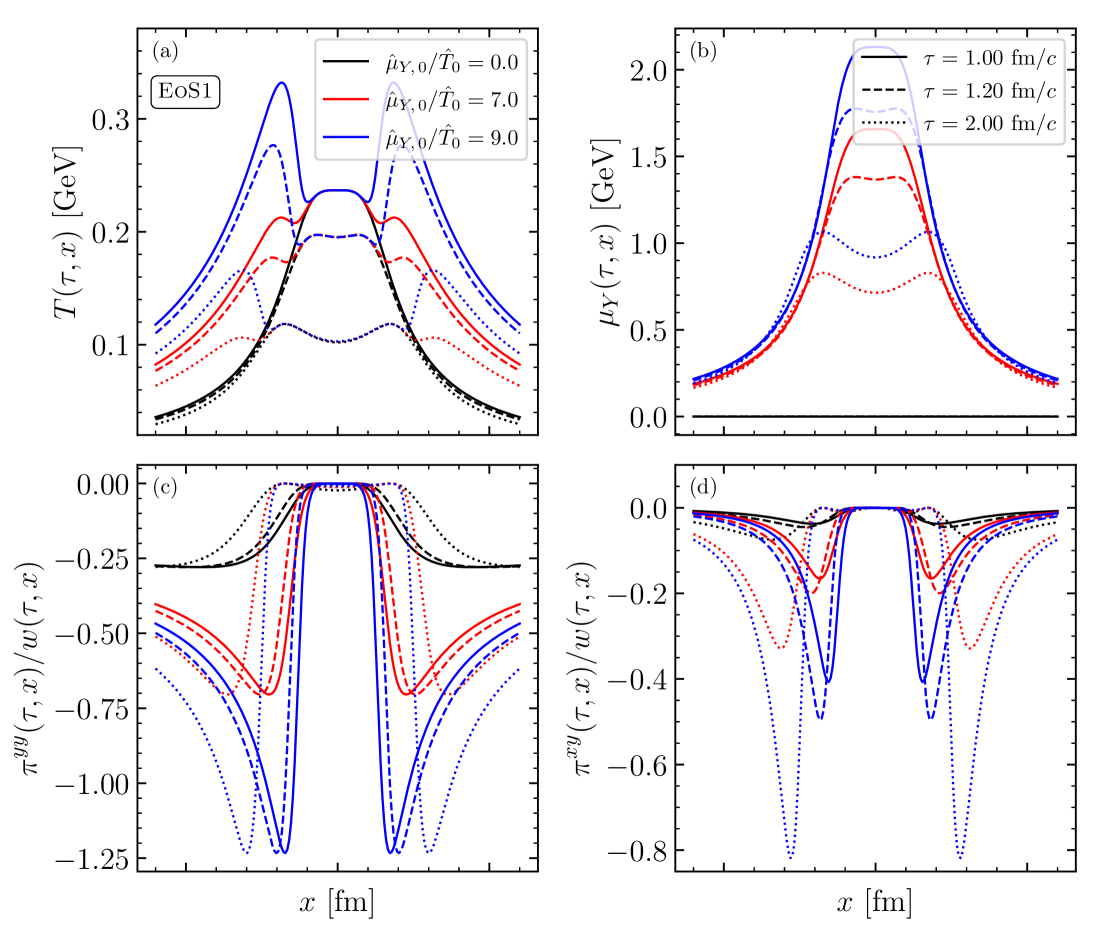
Figure 1: (Color online) We plot the semi-analytical solutions for Gubser flow with conserved charges in the plane $y=0$ (except $\pi^{xy}$, which is plotted in the plane $y=x$). Included are (a) the temperature, (b) chemical potential, (c) the dimensionless quantity $\pi^{yy}/w$, where $w=\mathcal{E}+\mathcal{P}$ is the enthalpy density, for a diagonal entry of the shear stress tensor, and (d) the dimensionless quantity $\pi^{xy}/w$ for an off-diagonal entry. The three different colors correspond to different initial conditions for the ratio of initial temperature and initial chemical potential: $\hat{\mu}_{Y,0}/\hat{T}_{0}=0$ (black), $7$ (red), $9$ (blue). The different types of lines correspond to selected times $\tau=1.0$ fm/$c$ (solid lines), $1.2$ fm/$c$ (dashed lines) and $2.0$ fm/$c$ (dotted lines) during the evolution. See text for discussion.

The energy density, number density, and entropy density, corresponding to the semi-analytical solution in Fig. 1, have been plotted in Fig. 2. Due to the decoupled evolution of the number density in VGCC, the qualitative behavior of quickly decaying of away from the core is independent of equation of state. Changing the initial condition $\hat{\mu}_{Y,0}/\hat{T}_{0}$ in the equation of state only results in shifting the profile of the number density in Fig. 2(b) up or down in magnitude but does not change its shape. Contrasting this to the equation of state and shear stress variables in Fig. 1, we find that the shear entries and temperature profiles are significantly more sensitive to our choice in $\hat{\mu}_{Y,0}/\hat{T}_{0}$.

We can also compare the spatial evolution of $\mu_{Y}$ in Fig.  1(b) to the spatial evolution of the number density $n_{Y}$ in Fig. 2(b). Away from the core the combined quantity $\mu_{Y}n_{Y}$ vanishes quickly such that $sT$ has to compensate to maintain the equality within the Gibbs-Duhem relation shown in Eq. (15), leading to the formation of shoulders observed in the entropy density, and consequently, the temperature. This increase in entropy, and consequently, increase of temperature is due to entropy production from the very large viscous corrections at finite chemical potential. In the absence of a chemical potential these shoulders cannot form, regardless of how large $\hat{\bar{\pi}}_{0}$ is.

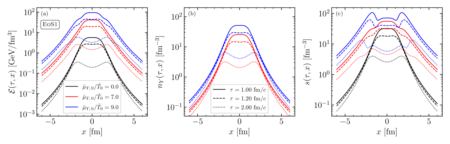
Figure 2: (Color online) We plot (a) the energy density, (b) number density, and (c) entropy density corresponding to the semi-analytical solutions for viscous Gubser flow with conserved charges shown in Fig. 1 in the plane $y=0$. We include the results for differential values of the initial conditions and at different times (see the caption of Fig. 1 for details). The number density plot does not feature black lines because at $\hat{\mu}_{Y,0}/\hat{T}_{0}=0$ the system has exactly vanishing number densities such that there is no evolution of the number density. Most notably, an increase in chemical potential can significantly decrease spatial variations of the energy density and entropy. The entropy density is most sensitive to the details of the temperature profile, as can be seen by the presence of the shoulders for the blue lines ($\hat{\mu}_{Y,0}/\hat{T}_{0}=9$).

IV.2 Freeze-out and entropy production

The freeze-out hypersurfaces for different initial conditions $\hat{\mu}_{Y,0}/\hat{T}_{0}$ and freeze-out energy density $\mathcal{E}_{\text{FO}}=1$ GeV/fm³ are shown in Fig. 3(a). Conformal symmetry requires the energy density to be proportional to $T^{4}$. At $\mu_{Y}=0$, this implies that the freeze-out hypersurface is isothermal and isentropic. However, for $\mu_{Y}\neq 0$, freeze-out is neither isothermal nor isentropic. Figure 3(a) shows that the entropy density (indicated by the color of the line and the color bar) close to the core is lower than the tails, i.e., freeze-out is no longer isentropic. This follows, again, from the Gibbs-Duhem relation in Eq. 15: The left-hand side is fixed by the freeze-out condition, while on the right-hand side, since the $n_{Y}\mu_{Y}$ term vanishes at the edge of the system, the entropy (per conserved number density) has to increase to satisfy the equality.

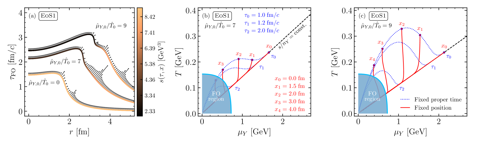
Figure 3: (Color online) We plot (a) the freeze-out hypersurface and normal vectors, and $T$ versus $\mu_{Y}$ trajectories for two initial conditions, (b) $\hat{\mu}_{Y,0}/\hat{T}_{0}=7$ and (c) $\hat{\mu}_{Y,0}/\hat{T}_{0}=9$ with $\hat{T}_{0}=1.2$. Included in the freeze-out hypersurface plot is a color bar which indicates the entropy density for a freeze-out cell at a given $(\tau_{\mathrm{FO}},r)$. As expected, at zero chemical potential, the freeze-out hypersurface is isentropic. At non-vanishing chemical potential, the entropy in the core is lower (i.e., lower temperature) than the entropy at the tails. To allow the normal vectors and freeze-out hypersurface on the screen, they have been rescaled by a factor of $0.075$.

The normal vectors to the freeze-out hypersurface are also presented in Fig. 3(a), where they have been rescaled by a factor of 0.075 to fit in the figure. Causality requires all normal vectors to be future directed, which is satisfied in all the cases considered. The divergences in normal vectors occur when the spatial and temporal variations of the energy density are close in magnitude.

In the middle and right panels of Fig. 3, we show the trajectories through the $T$ versus $\mu_{Y}$ plane, for two initial conditions $\hat{\mu}_{Y,0}/\hat{T}_{0}=7$ (middle) and $\hat{\mu}_{Y,0}/\hat{T}_{0}=9$ (right). The trajectories start at the top of the plot (on the fixed proper time surface with $\tau_{0}$ or fixed spatial coordinates $x$) and downwards in time. Because the Gubser flow is composed of a field that spans multiple different values of $T-\mu_{Y}$ for a single set of initial conditions, we show a number of selected trajectories for different points in space. Here, the blue dotted lines follow the profile of $(T,\mu_{Y})$ at a fixed proper time $\tau$ and red solid lines are the trajectories along the phase diagram at a fixed point in space. Notice how the shoulders seen for larger initial values $\hat{\mu}_{Y,0}/\hat{T}_{0}$ in the temperature profile of Fig. 1(a) enlarge the phase space probed (comparing the larger values and phase space in the right most figure vs the middle figure). The blue shaded area marks the region where the energy density falls below the threshold $\mathcal{E}_{\mathrm{FO}}$, while the black dashed line represents the isentropic trajectory where $s/n_{Y}=\text{const.}$ and is fixed at freeze-out. At early times the range of $T$ and $\mu_{Y}$ reached are to the left of the isentropic expansion, reaching lower chemical potentials $\mu_{Y}$ and either hotter or lower temperatures $T$, depending on the initial conditions. In addition, we also study the $(T,\mu_{Y})$ evolution of a given point in the fluid, i.e., the trajectories at constant $x$ position. Interestingly enough, at a fixed spatial position the fluid remains at a nearly fixed $\mu_{Y}$ but only cools over time.

These trajectories are dramatically different from those observed in Refs. [43, 41, 14, 40] for realistic equations of state based on lattice QCD matched to a hadron resonance gas, which have a negative slope close to the origin and bend in the opposite direction. The slope of these realistic EoS trajectories can be connected to a softening of the EoS close to the phase transition such that the speed of sound $c_{s}^{2}(T)$ reaches a minimum or, in other words, $\mathcal{P}(\mathcal{E})$ has a softer slope. Nonetheless, in a conformal system $\mathcal{E}=3\mathcal{P}$ and $c_{s}^{2}=1/3$ such that no softening occurs at hadronization and there is no bend in the isentropic trajectories. Instead, our isentropic trajectories start at high $T$, high $\mu_{Y}$ and then steadily decrease by in $T$ and $\mu_{Y}$ over time.

In an out-of-equilibrium, non-conformal system it has been previously shown that the deviation from isentropes ($s/n_{B}$), in terms of the passage through the $T-\mu_{B}$ plane, is significantly more complex due to higher-order terms in the hydrodynamic equations of motion and the complex interplay between shear and bulk viscosities [20, 21, 22]. Here, even though our equation of state is significantly more simplistic, we still find more complex behavior of the out-of-equilibrium fluid over time. It would be interesting to study the temporal vs spatial evolution of a realistic EoS at finite $\mu_{Y}$ in future work.

V Comparisons of ccake to the Gubser test

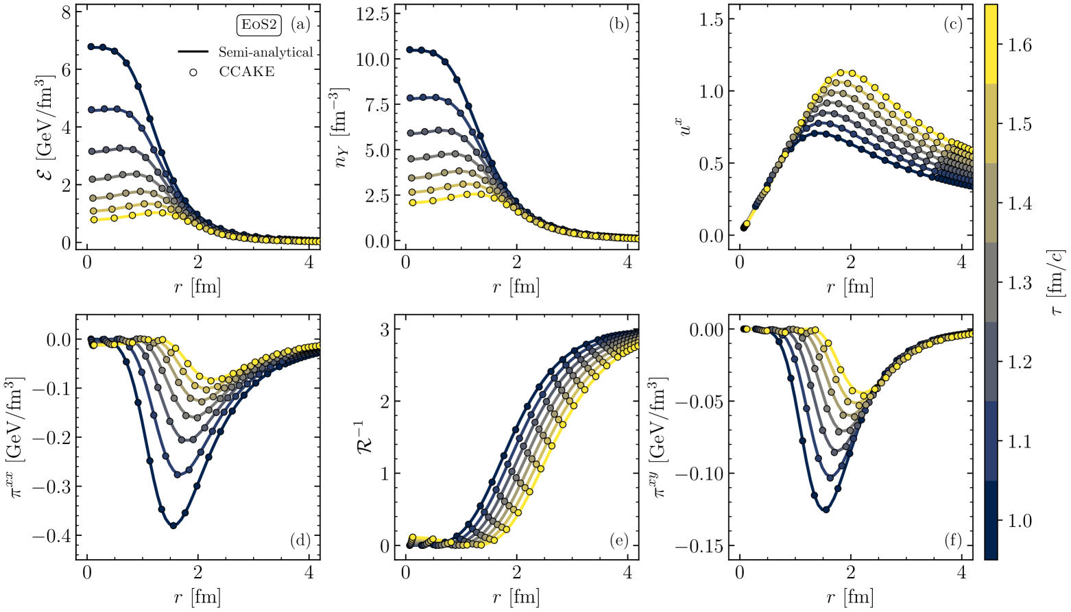
Figure 4: (Color online) We plot the numerical solution from the ccake code (dots) and semi-analytical solution (solid line) using EoS2 in Eq. (13) as a function of distance from the origin and for various time steps (indicated by the color bar) within the first fm/$c$ of evolution. The comparison is made between (a) energy density, (b) number density, (c) the $x$-component of the fluid velocity, (d) the $xx$-component of the shear stress tensor, (e) the inverse Reynolds number defined in Eq. (29), and (f) the $xy$-component of the shear stress tensor. We see excellent agreement for all shown variables with a very mild deviation of around a percent around the core for the energy density and number density. For the $xx$-component of the shear stress tensor, we also observe an increasing deviation of the numerical solution from the semi-analytical one for increasing time, specifically between $r=1$ fm and $r=2$ fm, with the maximum relative deviations at $\tau=1.6$ fm/$c$ getting large since the numerical solution is very close to zero. The largest deviations are seen on the $xy$-component of the shear stress tensor between $r=1$ fm and $r=2$ fm, and also present to a lesser extent on the diagonal component.

In the following section, we will use VGCC to benchmark the numerical solution of a hydrodynamic system with conserved charges implemented in the open source (2+1)-dimensional hydrodynamic code, Conserved Charge Hydrodynamik Evolution (ccake 1.0.0) [26]. ccake relies on the SPH computational method, which discretizes the fluid into individual particles (known as SPH particles) and simplifies the calculation of terms in the equations of motion. The individual SPH particles move with the fluid such that one tracks their dynamical degrees of freedom (e.g., position, velocity, and entropy) over time. At each time step, a nearest neighbor search is used to evaluate the equation of motion. For the time-integration scheme, we use 2${}^{\text{nd}}$-order Runge-Kutta (RK2), which has been tested against other methods and was found to optimize both accuracy and speed. Previously, it was shown that ccake 1.0.0 passed both the viscous Gubser test at vanishing densities and the ideal Gubser test at finite densities [26], but there was no test that combined both finite densities and viscosity, which is why we developed VGCC in this work.

To compare with VGCC, we insert the semi-analytical solutions from Eq. 19 with initial conditions

$$\hat{T}_{0}=1.2,\quad\frac{\hat{\mu}_{Y,0}}{\hat{T}_{0}}=0.3,\quad\hat{\bar{\pi}}_{0}=0,$$ (28)

into ccake and start our hydrodynamic evolution at $\tau_{0}=1.0\;\text{fm}/c$. The grid size is $x,y\in[-5,5]$ fm with a spacing of $0.05$ fm. We place an SPH particle on each grid point, which leads to a total of 40,401 SPH particles in each of these simulations. The smoothing scale is set to $h=0.1$ fm to account for the large gradients in Gubser flow. The equation of state used is EoS2 and is given in Eq. 13. Table 1 summarizes the initial conditions, equation of state, and ccake parameters used. The same VGCC parameters must be used in ccake for an appropriate comparison. For instance, in VGCC we set the specific shear viscosity to $\bar{\eta}\equiv\eta/s=0.2$, which also must be used in ccake.

VGCC parameters
$\tau_{0}$	1.0 fm/$c$
$\hat{T}_{0}$	1.2
$\hat{\mu}_{Y,0}/\hat{T}_{0}$	0.3
$\hat{\bar{\pi}}_{0}$	0.0
$\mathcal{E}_{\text{FO}}$	1 GeV/fm3
$\bar{\eta}=\eta/s$	0.20
$\tau_{R}$	Eq. 7
EoS parameters
EoS	EoS2 [Eq. 13]
$\mu_{\ast}$	1 GeV
$T_{\ast}$	1 GeV
ccake parameters
$h$	0.1 fm
$\delta x$, $\delta y$	0.05 fm
$\delta\tau$	0.001 fm/$c$

Table 1: Parameters used to define the semi-analytical solutions for VGCC, equation of state choice and parameters (middle), and ccake only parameters that determine the numerical accuracy (bottom) for comparisons. The same VGCC parameters and EoS must be used be used in both the semi-analytical solution and in ccake for direct comparisons.

Given the initial conditions discussed above, we compare the evolution calculated by ccake with the solution predicted by our semi-analytical solution. This comparison is presented in Fig. 4 where we present the energy density $\mathcal{E}$, a generic number density $n_{Y}$, $x$-component of the fluid velocity $u^{x}$, $xx$-component and $xy$-components of the shear stress tensor $\pi^{xx}$ and $\pi^{xy}$, and the inverse Reynolds number $\mathcal{R}^{-1}$ which we define as [58, Eq. 8.10]

$$\mathcal{R}^{-1}=\frac{\sqrt{\pi^{\mu\nu}\pi_{\mu\nu}}}{\mathcal{P}}\,.$$ (29)

We plot these quantities for multiple time steps as a function of the distance from the origin up to times of $\tau=1.6\;\text{fm}/c$, shown in Fig. 4. Figure 4 shows an excellent agreement overall between the semi-analytical and numerical solutions with minor deviations seen on $\pi^{xy}$ at late times at distances between 1 fm and 2 fm from the origin. The simulations were run until they failed which is signaled by the presence of SPH particles with negative entropy. We reached failure at $\sim 1.85$ fm/$c$, as expected from previous numerical tests for ccake [26] and its previous version v-USPhydro [59, 60]. Note that unlike most grid-based codes, we do not include any regulator within SPH (for discussions on regulators see [61, 62]).

The inverse Reynolds number, $\mathcal{R}^{-1}$, parametrizes how far from equilibrium a hydrodynamic system is. Large $\mathcal{R}^{-1}$ indicates that the viscous contributions dominate and signals the breakdown of hydrodynamics (for examples of values regularly reached in heavy-ion collisions see [63, 64, 65]). Large $\mathcal{R}^{-1}$, in turn, leads to numerical instabilities which can cause the entropy density to become negative. The size of the viscous corrections are also limited by causality [66, 67, 62, 68] and stability [46] (that implies causality [69]). Causality violations are manifest at distances of $r\approx 1.5–2.5\;\text{fm}$ away from the center and at late times, as demonstrated by Fig. 1(c). In addition, causality violations are inherently linked to large $\mathcal{R}^{-1}$, hence we can conclude from Fig. 4(e) that the system at large radii (and early times) is likely well beyond causal constraints as well. We do find that ccake can correctly describe even very large values of $\mathcal{R}^{-1}$, but the eventual discrepancies and crashing of ccake at late times is likely due to far-from-equilibrium behavior in other regions of the fluid. Because ccake is based on an SPH algorithm, the SPH particles move in time such that Fig. 4 only shows their results in a snapshot in time, but they could have previously been in a part of the fluid that was far-from-equilibrium. Thus, far-from-equilibrium behavior certainly leads to the breakdown of hydrodynamics but it is not clear yet where in the fluid this breakdown starts, only where it ends.

As noted, late times eventually lead to a crash in ccake due to far-from-equilibrium and acausal behavior. A natural question that arises is if this concerning behavior appears before or after the conversion of fluid dynamics into a hadron resonance gas phase. The good news is that one can systematically check the freeze-out hypersurface against the semi-analytical solution derived from the Gubser test, which we do next. We find that all fluid cells freeze-out before ccake crashes, implying that the problematic behavior only occurs at low temperatures, outside the regime where we expect hydrodynamics to be relevant.

Within ccake, the freeze-out hypersurface is calculated directly from the SPH particle information as one crosses the freeze-out criteria (either fixed temperature or energy density). However, as anticipated in Sec. III, due to finite time steps $\delta\tau$ one almost never hits the freeze-out criteria exactly, but is either slightly above or below; ccake picks the result that minimizes the distance from the freeze-out criteria. With such an algorithm, the smaller the choice of $\delta\tau$, the more accurate the freeze-out hypersurface.

A comparison between the freeze-out hypersurface predicted by ccake and the one calculated by VGCC is made in Fig. 5. We see excellent agreement between the two. Thus, this confirms that our approach to obtaining the hypersurface works well and is numerically accurate. Additionally, we find that for the Gubser test the breakdown of hydrodynamics occurs outside of the regime where we expect the system to behave as a fluid.

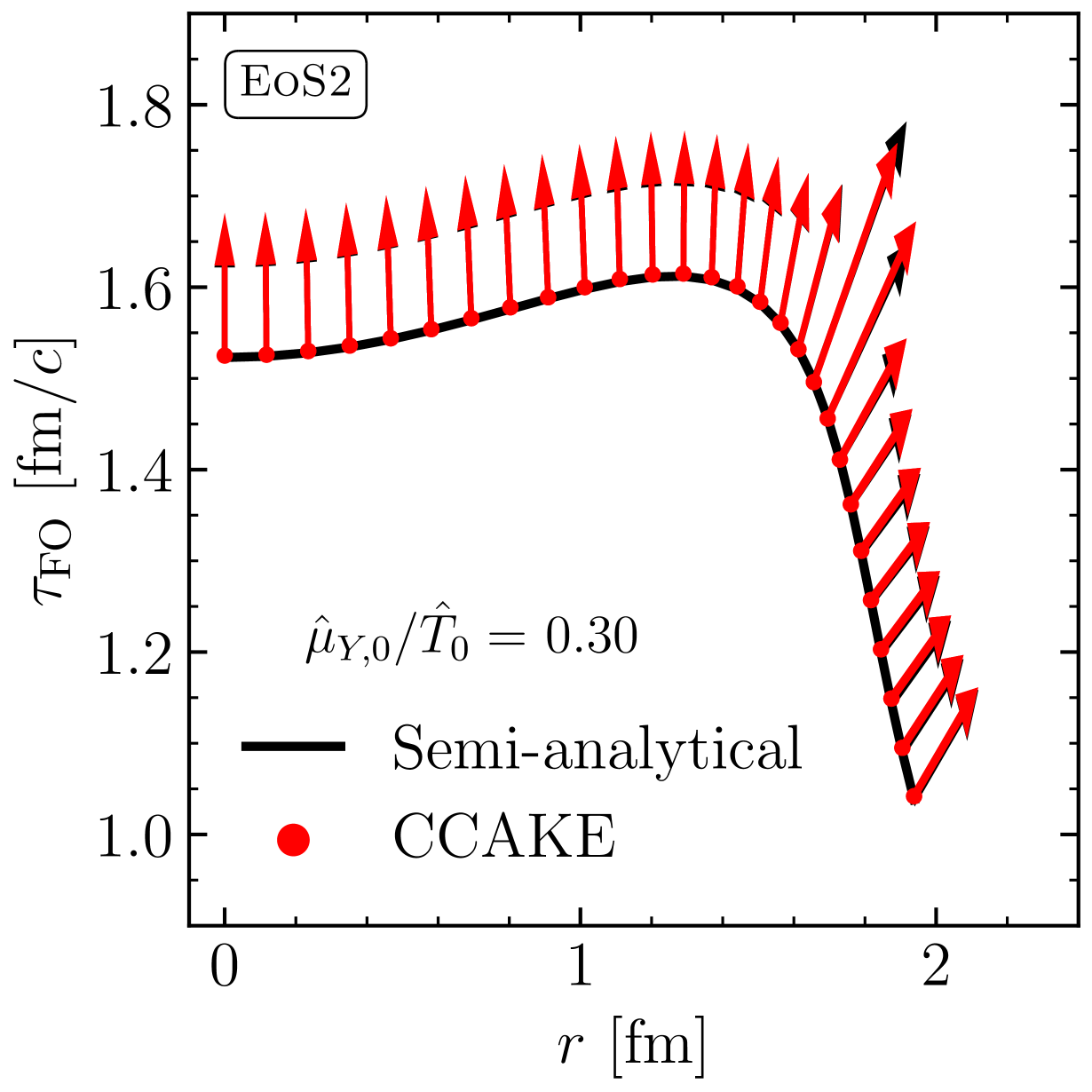
Figure 5: (Color online) A comparison between the freeze-out hypersurface and normal vectors obtained from ccake (red) and the semi-analytical solution for VGCC (black). We see a slight disagreement on the magnitude of the (close to) divergent normal vectors. This disagreement is likely a result of the SPH particles freezing-out a time-step after the actual freeze-out time within the simulation.

VI Conclusion

In this paper we provided the first study of the evolution of both the temperature and chemical potentials for viscous hydrodynamics systems with conserved currents undergoing Gubser flow. We found that the addition of a chemical potential (as in contrast to $\mu_{Y}=0$) can push the fluid significantly further from equilibrium, dramatically changing the temperature and energy density profiles in the process. Our work allowed us to study out-of-equilibrium trajectories in a system with semi-analytical solutions to better understand its spacetime evolution. Compared to $\mu_{Y}=0$, we find that the $\mu_{Y}\neq 0$ evolution leads to particles at freeze-out that are significantly more boosted as indicated by the longer normal vectors on the freeze-out hypersurface.

The viscous Gubser flow with conserved charges (VGCC) solution provides a benchmark for hydrodynamics codes with conserved charges, such as ccake. We showed that ccake passed our new Gubser test up until times of $\tau=\tau_{\text{lim}}\sim 1.85$ fm/$c$. At times after $\tau_{\text{lim}}$, ccake crashes due to far-from-equilibrium effects that lead to negative entropy in certain SPH particles. However, we find that the fluid has already reached the freeze-out temperature by this time such that we can make direct comparisons between the VGCC and ccake hypersurfaces. Lastly, we show that ccake can very accurately reproduce the hypersurface generated using via Gubser flow.

Further development of the ideas presented here would help bridge exact solutions and heavy-ion experimental results. For example, the inclusion of a critical point on the EoS used would help elucidate exactly how a critical point affects the fluid in neighboring regions of the phase diagram. Another interesting avenue is the implementation of a Gubser flow solution of relativistic viscous fluids in 3+1D with conserved charges, which would provide a helpful tool in the context of low and medium beam energies, where the chemical potentials probed are expected to be the largest.

Appendix A de Sitter-to-Milne transformations

In this appendix, we present explicit expressions for the coordinate transformation of the shear stress tensor in Milne coordinates. In the below, all quantities with hats are in de Sitter coordinate, while un-hatted quantities are in Milne coordinates. Recall that $\pi_{\mu\nu}$ is diagonal in de Sitter coordinates,

$$\hat{\pi}_{\mu\nu}=-\frac{\hat{\pi}}{2}\mathrm{diag}(0,\cosh^{2}\rho,\cosh^{2}\rho\sin^{2}\theta,-2).$$ (30)

To transform these to Milne coordinates, we will need the identities

$$\left(\frac{\partial\theta}{\partial\tau}\right)^{2}\cosh^{2}{\rho} =\frac{u_{r}^{2}}{\tau^{2}},$$ (31a)

$$\frac{\partial\theta}{\partial\tau}\frac{\partial\theta}{\partial r}\cosh^{2}{\rho} =\frac{1}{\tau^{2}}u_{r}u_{\tau},$$ (31b)

$$\left[\left(\frac{\partial\theta}{\partial r}\right)^{2}-\frac{\sin^{2}\theta}{r^{2}}\right]\cosh^{2}\rho =\frac{u_{r}^{2}}{\tau^{2}},$$ (31c)

$$\left[x^{2}\left(\frac{\partial\theta}{\partial r}\right)^{2}-\frac{y^{2}}{r^{2}}\sin^{2}\theta\right]\cosh^{2}\rho =\frac{r^{2}}{\tau^{2}}\left(1+\frac{x^{2}}{r^{2}}u_{r}^{2}\right),$$ (31d)

where $\theta$ and $\rho$ are defined in Eqs. (18) and $u_{r}$ and $u_{\tau}$ are given in Eqs. (2). Lastly, we note that $u_{x}=(x/r)u_{r}$. Therefore,

$$\pi_{\mu\nu}=-\frac{\hat{\pi}}{2\tau^{4}}\begin{pmatrix}u_{r}^{2}&u_{x}u_{\tau}&u_{y}u_{\tau}&\\ &1+u_{x}^{2}&u_{x}u_{y}&\\ &&1+u_{y}^{2}&\\ &&&-2\tau^{2}\end{pmatrix}.$$ (32)

References

- Heinz and Snellings [2013] U. Heinz and R. Snellings, Collective flow and viscosity in relativistic heavy-ion collisions, Ann. Rev. Nucl. Part. Sci. 63, 123 (2013), arXiv:1301.2826 [nucl-th] .
- Luzum and Petersen [2014] M. Luzum and H. Petersen, Initial State Fluctuations and Final State Correlations in Relativistic Heavy-Ion Collisions, J. Phys. G 41, 063102 (2014), arXiv:1312.5503 [nucl-th] .
- Derradi de Souza et al. [2016] R. Derradi de Souza, T. Koide, and T. Kodama, Hydrodynamic Approaches in Relativistic Heavy Ion Reactions, Prog. Part. Nucl. Phys. 86, 35 (2016), arXiv:1506.03863 [nucl-th] .
- Romatschke and Romatschke [2019] P. Romatschke and U. Romatschke, Relativistic Fluid Dynamics In and Out of Equilibrium, Cambridge Monographs on Mathematical Physics (Cambridge University Press, 2019) arXiv:1712.05815 [nucl-th] .
- Bjorken [1983] J. D. Bjorken, Highly Relativistic Nucleus-Nucleus Collisions: The Central Rapidity Region, Phys. Rev. D 27, 140 (1983).
- Gubser [2010] S. S. Gubser, Symmetry constraints on generalizations of Bjorken flow, Phys. Rev. D 82, 085027 (2010), arXiv:1006.0006 [hep-th] .
- Gubser and Yarom [2011] S. S. Gubser and A. Yarom, Conformal hydrodynamics in Minkowski and de Sitter spacetimes, Nucl. Phys. B 846, 469 (2011), arXiv:1012.1314 [hep-th] .
- Shi et al. [2022] S. Shi, S. Jeon, and C. Gale, Family of new exact solutions for longitudinally expanding ideal fluids, Phys. Rev. C 105, L021902 (2022), arXiv:2201.06670 [hep-ph] .
- Bradley and Plumberg [2024] O. Bradley and C. Plumberg, Exploring freeze-out and flow using exact solutions of conformal hydrodynamics, Phys. Rev. C 109, 054913 (2024), arXiv:2402.03568 [nucl-th] .
- Baym et al. [2018] G. Baym, T. Hatsuda, T. Kojo, P. D. Powell, Y. Song, and T. Takatsuka, From hadrons to quarks in neutron stars: a review, Rept. Prog. Phys. 81, 056902 (2018), arXiv:1707.04966 [astro-ph.HE] .
- Busza et al. [2018] W. Busza, K. Rajagopal, and W. van der Schee, Heavy Ion Collisions: The Big Picture, and the Big Questions, Ann. Rev. Nucl. Part. Sci. 68, 339 (2018), arXiv:1802.04801 [hep-ph] .
- Bzdak et al. [2020] A. Bzdak, S. Esumi, V. Koch, J. Liao, M. Stephanov, and N. Xu, Mapping the Phases of Quantum Chromodynamics with Beam Energy Scan, Phys. Rept. 853, 1 (2020), arXiv:1906.00936 [nucl-th] .
- Dexheimer et al. [2021] V. Dexheimer, J. Noronha, J. Noronha-Hostler, C. Ratti, and N. Yunes, Future physics perspectives on the equation of state from heavy ion collisions to neutron stars, J. Phys. G 48, 073001 (2021), arXiv:2010.08834 [nucl-th] .
- Monnai et al. [2021] A. Monnai, B. Schenke, and C. Shen, QCD Equation of State at Finite Chemical Potentials for Relativistic Nuclear Collisions, Int. J. Mod. Phys. A 36, 2130007 (2021), arXiv:2101.11591 [nucl-th] .
- An et al. [2022] X. An et al., The BEST framework for the search for the QCD critical point and the chiral magnetic effect, Nucl. Phys. A 1017, 122343 (2022), arXiv:2108.13867 [nucl-th] .
- Lovato et al. [2022] A. Lovato et al., Long Range Plan: Dense matter theory for heavy-ion collisions and neutron stars, (2022), arXiv:2211.02224 [nucl-th] .
- Achenbach et al. [2024] P. Achenbach et al., The present and future of QCD, Nucl. Phys. A 1047, 122874 (2024), arXiv:2303.02579 [hep-ph] .
- Sorensen et al. [2024] A. Sorensen et al., Dense nuclear matter equation of state from heavy-ion collisions, Prog. Part. Nucl. Phys. 134, 104080 (2024), arXiv:2301.13253 [nucl-th] .
- Du et al. [2024] L. Du, A. Sorensen, and M. Stephanov, The QCD phase diagram and Beam Energy Scan physics: a theory overview, Int. J. Mod. Phys. E 33, 2430008 (2024), arXiv:2402.10183 [nucl-th] .
- Dore et al. [2020] T. Dore, J. Noronha-Hostler, and E. McLaughlin, Far-from-equilibrium search for the QCD critical point, Phys. Rev. D 102, 074017 (2020), arXiv:2007.15083 [nucl-th] .
- Dore et al. [2022] T. Dore, J. M. Karthein, I. Long, D. Mroczek, J. Noronha-Hostler, P. Parotto, C. Ratti, and Y. Yamauchi, Critical lensing and kurtosis near a critical point in the QCD phase diagram in and out of equilibrium, Phys. Rev. D 106, 094024 (2022), arXiv:2207.04086 [nucl-th] .
- Chattopadhyay et al. [2023] C. Chattopadhyay, U. Heinz, and T. Schaefer, Far-off-equilibrium expansion trajectories in the QCD phase diagram, Phys. Rev. C 107, 044905 (2023), arXiv:2209.10483 [hep-ph] .
- Du and Schlichting [2021] X. Du and S. Schlichting, Equilibration of the Quark-Gluon Plasma at Finite Net-Baryon Density in QCD Kinetic Theory, Phys. Rev. Lett. 127, 122301 (2021), arXiv:2012.09068 [hep-ph] .
- Pradeep et al. [2024] M. S. Pradeep, N. Sogabe, M. Stephanov, and H.-U. Yee, Nonmonotonic specific entropy on the transition line near the QCD critical point, Phys. Rev. C 109, 064905 (2024), arXiv:2402.09519 [nucl-th] .
- Denicol et al. [2018] G. S. Denicol, C. Gale, S. Jeon, A. Monnai, B. Schenke, and C. Shen, Net baryon diffusion in fluid dynamic simulations of relativistic heavy-ion collisions, Phys. Rev. C 98, 034916 (2018), arXiv:1804.10557 [nucl-th] .
- Plumberg et al. [2024] C. Plumberg et al., BSQ Conserved Charges in Relativistic Viscous Hydrodynamics solved with Smoothed Particle Hydrodynamics, (2024), arXiv:2405.09648 [nucl-th] .
- Du and Heinz [2020] L. Du and U. Heinz, (3+1)-dimensional dissipative relativistic fluid dynamics at non-zero net baryon density, Comput. Phys. Commun. 251, 107090 (2020), arXiv:1906.11181 [nucl-th] .
- Hatta et al. [2015] Y. Hatta, A. Monnai, and B.-W. Xiao, Flow harmonics at finite density, Phys. Rev. D 92, 114010 (2015), arXiv:1505.04226 [hep-ph] .
- Hatta et al. [2014] Y. Hatta, J. Noronha, G. Torrieri, and B.-W. Xiao, Flow harmonics within an analytically solvable viscous hydrodynamic model, Phys. Rev. D 90, 074026 (2014), arXiv:1407.5952 [hep-ph] .
- Hiscock and Lindblom [1985] W. A. Hiscock and L. Lindblom, Generic instabilities in first-order dissipative relativistic fluid theories, Phys. Rev. D 31, 725 (1985).
- [31] https://the-nuclear-confectionery.github.io/ccake-site/.
- Landau and Lifshitz [1987] L. D. Landau and E. M. Lifshitz, Fluid Mechanics, 2nd ed., Course of Theoretical Physics, Vol. 6 (Butterworth-Heinemann, 1987) p. 552.
- Marrochio et al. [2015] H. Marrochio, J. Noronha, G. S. Denicol, M. Luzum, S. Jeon, and C. Gale, Solutions of Conformal Israel-Stewart Relativistic Viscous Fluid Dynamics, Phys. Rev. C 91, 014903 (2015), arXiv:1307.6130 [nucl-th] .
- Baier et al. [2008] R. Baier, P. Romatschke, D. T. Son, A. O. Starinets, and M. A. Stephanov, Relativistic viscous hydrodynamics, conformal invariance, and holography, JHEP 04, 100, arXiv:0712.2451 [hep-th] .
- Greif et al. [2018] M. Greif, J. A. Fotakis, G. S. Denicol, and C. Greiner, Diffusion of conserved charges in relativistic heavy ion collisions, Phys. Rev. Lett. 120, 242301 (2018), arXiv:1711.08680 [hep-ph] .
- Fotakis et al. [2020] J. A. Fotakis, M. Greif, C. Greiner, G. S. Denicol, and H. Niemi, Diffusion processes involving multiple conserved charges: A study from kinetic theory and implications to the fluid-dynamical modeling of heavy ion collisions, Phys. Rev. D 101, 076007 (2020), arXiv:1912.09103 [hep-ph] .
- Oliinychenko and Koch [2019] D. Oliinychenko and V. Koch, Microcanonical Particlization with Local Conservation Laws, Phys. Rev. Lett. 123, 182302 (2019), arXiv:1902.09775 [hep-ph] .
- Oliinychenko et al. [2020] D. Oliinychenko, S. Shi, and V. Koch, Effects of local event-by-event conservation laws in ultrarelativistic heavy-ion collisions at particlization, Phys. Rev. C 102, 034904 (2020), arXiv:2001.08176 [hep-ph] .
- Carzon et al. [2023] P. Carzon, M. Martinez, J. Noronha-Hostler, P. Plaschke, S. Schlichting, and M. Sievert, Pre-equilibrium evolution of conserved charges with initial conditions in the ICCING Monte Carlo event generator, Phys. Rev. C 108, 064905 (2023), arXiv:2301.04572 [nucl-th] .
- Monnai et al. [2019] A. Monnai, B. Schenke, and C. Shen, Equation of state at finite densities for QCD matter in nuclear collisions, Phys. Rev. C 100, 024907 (2019), arXiv:1902.05095 [nucl-th] .
- Noronha-Hostler et al. [2019] J. Noronha-Hostler, P. Parotto, C. Ratti, and J. M. Stafford, Lattice-based equation of state at finite baryon number, electric charge and strangeness chemical potentials, Phys. Rev. C 100, 064910 (2019), arXiv:1902.06723 [hep-ph] .
- Bellwied et al. [2020] R. Bellwied, S. Borsanyi, Z. Fodor, J. N. Guenther, J. Noronha-Hostler, P. Parotto, A. Pasztor, C. Ratti, and J. M. Stafford, Off-diagonal correlators of conserved charges from lattice QCD and how to relate them to experiment, Phys. Rev. D 101, 034506 (2020), arXiv:1910.14592 [hep-lat] .
- Karthein et al. [2021] J. M. Karthein, D. Mroczek, A. R. Nava Acuna, J. Noronha-Hostler, P. Parotto, D. R. P. Price, and C. Ratti, Strangeness-neutral equation of state for QCD with a critical point, Eur. Phys. J. Plus 136, 621 (2021), arXiv:2103.08146 [hep-ph] .
- Aryal et al. [2020] K. Aryal, C. Constantinou, R. L. S. Farias, and V. Dexheimer, High-Energy Phase Diagrams with Charge and Isospin Axes under Heavy-Ion Collision and Stellar Conditions, Phys. Rev. D 102, 076016 (2020), arXiv:2004.03039 [nucl-th] .
- Denicol et al. [2012] G. S. Denicol, H. Niemi, E. Molnar, and D. H. Rischke, Derivation of transient relativistic fluid dynamics from the Boltzmann equation, Phys. Rev. D 85, 114047 (2012), [Erratum: Phys.Rev.D 91, 039902 (2015)], arXiv:1202.4551 [nucl-th] .
- Almaalol et al. [2025] D. Almaalol, T. Dore, and J. Noronha-Hostler, Stability of multicomponent relativistic viscous hydrodynamics from Israel-Stewart and reproducing Denicol-Niemi-Molnar-Rischke from maximizing the entropy, Phys. Rev. D 111, 014020 (2025), arXiv:2209.11210 [hep-th] .
- Fotakis et al. [2022] J. A. Fotakis, E. Molnár, H. Niemi, C. Greiner, and D. H. Rischke, Multicomponent relativistic dissipative fluid dynamics from the Boltzmann equation, Phys. Rev. D 106, 036009 (2022), arXiv:2203.11549 [nucl-th] .
- Schäfer et al. [2022] A. Schäfer, I. Karpenko, X.-Y. Wu, J. Hammelmann, and H. Elfner (SMASH), Particle production in a hybrid approach for a beam energy scan of Au+Au/Pb+Pb collisions between = 4.3 GeV and = 200.0 GeV, Eur. Phys. J. A 58, 230 (2022), arXiv:2112.08724 [hep-ph] .
- Martinez et al. [2019] M. Martinez, M. D. Sievert, D. E. Wertepny, and J. Noronha-Hostler, Initial state fluctuations of QCD conserved charges in heavy-ion collisions, (2019), arXiv:1911.10272 [nucl-th] .
- Carzon et al. [2022] P. Carzon, M. Martinez, M. D. Sievert, D. E. Wertepny, and J. Noronha-Hostler, Monte Carlo event generator for initial conditions of conserved charges in nuclear geometry, Phys. Rev. C 105, 034908 (2022), arXiv:1911.12454 [nucl-th] .
- Chaudhuri [2014] A. K. Chaudhuri, Equation of state for qgp and hadronic resonance gas, in A Short Course on Relativistic Heavy Ion Collisions, 2053-2563 (IOP Publishing, 2014) pp. 6–1 to 6–20.
- Loganayagam [2008] R. Loganayagam, Entropy Current in Conformal Hydrodynamics, JHEP 05, 087, arXiv:0801.3701 [hep-th] .
- Alba et al. [2014] P. Alba, W. Alberico, R. Bellwied, M. Bluhm, V. Mantovani Sarti, M. Nahrgang, and C. Ratti, Freeze-out conditions from net-proton and net-charge fluctuations at RHIC, Phys. Lett. B 738, 305 (2014), arXiv:1403.4903 [hep-ph] .
- Bellwied et al. [2015] R. Bellwied, S. Borsanyi, Z. Fodor, J. Günther, S. D. Katz, C. Ratti, and K. K. Szabo, The QCD phase diagram from analytic continuation, Phys. Lett. B 751, 559 (2015), arXiv:1507.07510 [hep-lat] .
- Adamczyk et al. [2017] L. Adamczyk et al. (STAR), Bulk Properties of the Medium Produced in Relativistic Heavy-Ion Collisions from the Beam Energy Scan Program, Phys. Rev. C 96, 044904 (2017), arXiv:1701.07065 [nucl-ex] .
- Bellwied et al. [2019] R. Bellwied, J. Noronha-Hostler, P. Parotto, I. Portillo Vazquez, C. Ratti, and J. M. Stafford, Freeze-out temperature from net-kaon fluctuations at energies available at the BNL Relativistic Heavy Ion Collider, Phys. Rev. C 99, 034912 (2019), arXiv:1805.00088 [hep-ph] .
- Huovinen and Petersen [2012] P. Huovinen and H. Petersen, Particlization in hybrid models, Eur. Phys. J. A 48, 171 (2012), arXiv:1206.3371 [nucl-th] .
- Denicol and Rischke [2022] G. Denicol and D. Rischke, Microscopic Foundations of Relativistic Fluid Dynamics, Lecture Notes in Physics (Springer International Publishing, 2022).
- Noronha-Hostler et al. [2013] J. Noronha-Hostler, G. S. Denicol, J. Noronha, R. P. G. Andrade, and F. Grassi, Bulk Viscosity Effects in Event-by-Event Relativistic Hydrodynamics, Phys. Rev. C 88, 044916 (2013), arXiv:1305.1981 [nucl-th] .
- Noronha-Hostler et al. [2014] J. Noronha-Hostler, J. Noronha, and F. Grassi, Bulk viscosity-driven suppression of shear viscosity effects on the flow harmonics at energies available at the BNL Relativistic Heavy Ion Collider, Phys. Rev. C 90, 034907 (2014), arXiv:1406.3333 [nucl-th] .
- Shen et al. [2016] C. Shen, Z. Qiu, H. Song, J. Bernhard, S. Bass, and U. Heinz, The iEBE-VISHNU code package for relativistic heavy-ion collisions, Comput. Phys. Commun. 199, 61 (2016), arXiv:1409.8164 [nucl-th] .
- Chiu and Shen [2021] C. Chiu and C. Shen, Exploring theoretical uncertainties in the hydrodynamic description of relativistic heavy-ion collisions, Phys. Rev. C 103, 064901 (2021), arXiv:2103.09848 [nucl-th] .
- Niemi and Denicol [2014] H. Niemi and G. S. Denicol, How large is the Knudsen number reached in fluid dynamical simulations of ultrarelativistic heavy ion collisions?, (2014), arXiv:1404.7327 [nucl-th] .
- Noronha-Hostler et al. [2016] J. Noronha-Hostler, J. Noronha, and M. Gyulassy, Sensitivity of flow harmonics to subnucleon scale fluctuations in heavy ion collisions, Phys. Rev. C 93, 024909 (2016), arXiv:1508.02455 [nucl-th] .
- Summerfield et al. [2021] N. Summerfield, B.-N. Lu, C. Plumberg, D. Lee, J. Noronha-Hostler, and A. Timmins, 16O 16O collisions at energies available at the BNL Relativistic Heavy Ion Collider and at the CERN Large Hadron Collider comparing clustering versus substructure, Phys. Rev. C 104, L041901 (2021), arXiv:2103.03345 [nucl-th] .
- Bemfica et al. [2021] F. S. Bemfica, M. M. Disconzi, V. Hoang, J. Noronha, and M. Radosz, Nonlinear Constraints on Relativistic Fluids Far from Equilibrium, Phys. Rev. Lett. 126, 222301 (2021), arXiv:2005.11632 [hep-th] .
- Plumberg et al. [2022] C. Plumberg, D. Almaalol, T. Dore, J. Noronha, and J. Noronha-Hostler, Causality violations in realistic simulations of heavy-ion collisions, Phys. Rev. C 105, L061901 (2022), arXiv:2103.15889 [nucl-th] .
- Krupczak et al. [2024] R. Krupczak et al. (ExTrEMe), Causality violations in simulations of large and small heavy-ion collisions, Phys. Rev. C 109, 034908 (2024), arXiv:2311.02210 [nucl-th] .
- Gavassino et al. [2022] L. Gavassino, M. Antonelli, and B. Haskell, Thermodynamic Stability Implies Causality, Phys. Rev. Lett. 128, 010606 (2022), arXiv:2105.14621 [gr-qc] .