Also visitor at: ]Theoretical Physics Department, Fermi National Accelerator Laboratory, Batavia, Illinois 60510, USA

Testable dark matter solution within the seesaw mechanism

Abstract

The presence of a dark matter component in the Universe, together with the discovery of neutrino masses from the observation of the oscillation phenomenon, represents one of the most important open questions in particle physics today. A concurrent solution arises when one of the right-handed neutrinos, necessary for the generation of light neutrino masses, is itself the dark matter candidate. In this article, we study the generation of such a dark matter candidate relying solely on the presence of neutrino mixing. This tightly links the generation of dark matter with searches in laboratory experiments on top of the usual indirect dark matter probes. We find that the regions of parameter space producing the observed dark matter abundance can be probed indirectly with electroweak precision observables and charged lepton flavor violation searches. Given that the heavy neutrino masses need to lie at most around the TeV scale, probes at future colliders would further test this production mechanism.

Introduction: Despite its enormous success in predicting a wide range of experimentally tested phenomena, the Standard Model (SM) of particle physics has a number of known shortcomings, such as the origin of neutrino masses, the existence of a dark matter (DM) component in the Universe, and the generation of the baryon asymmetry (BAU), among others. A minimal extension of the SM simultaneously accommodating the aforementioned puzzles would be undoubtedly appealing.

Seesaw-based extensions of the SM potentially have these features, since right-handed (RH) neutrinos are responsible for the generation of neutrino masses and, under suitable conditions, represent viable DM candidates. Furthermore, they can account for the BAU via leptogenesis Fukugita and Yanagida (1986); Akhmedov et al. (1998); Davidson et al. (2008); Hernández et al. (2016); Abada et al. (2017); Sandner et al. (2023). To the best of our knowledge, the so-called $\nu$MSM Asaka et al. (2005); Asaka and Shaposhnikov (2005); Asaka et al. (2007); Shaposhnikov (2008); Laine and Shaposhnikov (2008) is the only seesaw scenario achieving, with a minimal field content, the generation of neutrino masses and the BAU, as well as having a DM candidate produced resonantly in the presence of lepton asymmetries Canetti et al. (2013); Ghiglieri and Laine (2019, 2020).

In this letter, we propose a different DM production mechanism, while complying with neutrino mass generation when introducing three RH neutrinos. In particular, the DM relic density is produced “à la” freeze-in through two body decays, without relying on any pre-existing lepton asymmetry. Moreover, the non-DM RH neutrinos need to lie at scales of the order of $100\,\mathrm{GeV}-1\,\mathrm{TeV}$ and have sizable couplings with the SM sector. While ensuring the effectiveness of the feeze-in mechanism, this feature places the viable parameter space in reach for future collider probes, such as FCC, and experiments searching for charged lepton flavor violation (cLFV).

The letter is organized as follows: we start by introducing the model and the generation of light neutrino masses. We then describe the DM production mechanism, in the context of thermal field theory (TFT), and the computation of its abundance. Next, we present current experimental constraints that need to be taken into account. Finally, we discuss our main results as well as future experimental prospects, and conclude.

Theoretical setup: We work in the context of the Type-I seesaw Minkowski (1977); Mohapatra and Senjanovic (1980); Yanagida (1979); Gell-Mann et al. (1979) with three RH neutrinos $N_{R_{i}}$, one of which represents the DM candidate with a mass $m_{\mathrm{DM}}\sim\mathcal{O}$(keV). The SM Lagrangian is completed by

$$\mathcal{L}\supset-\bar{L}_{L}\tilde{\Phi}Y_{\nu}N_{R}-\frac{1}{2}\bar{N}_{R}^{c}M_{N}N_{R}+h.c.\,,$$ (1)

where $L_{L}$ ($\Phi$) represents the $SU(2)_{L}$ lepton (Higgs) doublet and $Y_{\nu}$ is the neutrino Yukawa matrix. $M_{N}$ is the sterile neutrino Majorana mass term, which we assume real and diagonal without loss of generality. After electroweak (EW) spontaneous symmetry breaking (SSB), the light-neutrino masses, assuming $m_{D}\ll M_{N}$, are given by $m_{\nu}\simeq-m_{D}M_{N}^{-1}m_{D}^{T}$, where $m_{D}\equiv v_{H}Y_{\nu}/\sqrt{2}$ and $v_{H}$ denotes the Higgs vacuum expectation value (vev). We rewrite $m_{D}$ using the Casas-Ibarra (CI) parameterization:

$$m_{D}=-iU_{\mathrm{PMNS}}\sqrt{m_{d}}R^{T}\sqrt{M_{N}}\,,$$ (2)

where $U_{\mathrm{PMNS}}$ is the lepton mixing matrix measured in oscillation experiments, $m_{d}$ is the diagonal light-neutrino mass matrix and $R$ an orthogonal matrix, which can be parameterized with three rotations $V_{ij}$ in the $i-j$ plane, $R=V_{23}V_{13}V_{12}$, and thus by three complex angles $\vartheta_{ij}$. The CI parameterization guarantees the correct description of oscillation data Esteban et al. (2024) from the diagonalization of the full neutrino mass matrix. We will work in the limit of approximate lepton-number conservation Branco et al. (1989); Kersten and Smirnov (2007); Abada et al. (2007); Moffat et al. (2017); Lucente (2023), which allows for large active-heavy mixing angles, $U_{\alpha(i+3)}$ with $\alpha\in\{e,\,\mu,\,\tau\}$ and $i\in\{1,\,2,\,3\}$, while protecting light-neutrino masses from radiative corrections. The size of $U_{\alpha(i+3)}$ controls the strength of the interactions between the heavy mostly-sterile states and the rest of the SM, and it is approximately given by $U_{\alpha(i+3)}\simeq(m_{D}M_{N}^{-1})_{\alpha i}$. In the CI parameterization, and depending on the light-neutrino mass ordering, the lepton-number conserving limit is found for different values of $\vartheta_{12}$ and $\vartheta_{13}$ while having $\mathrm{Im}\left(\vartheta_{23}\right)\gg 1$. For normal ordering (NO), it corresponds to $\vartheta_{12},\,\vartheta_{13}\rightarrow 0$, while for inverted ordering (IO) it is realized when $\vartheta_{12},\,-\vartheta_{13}\rightarrow-\pi/2$.

In the lepton number conserving limit one naturally finds that the DM candidate interacts very weakly, $|\theta_{\alpha\mathrm{DM}}|\equiv|U_{\alpha 4}|\ll 1$, in agreement with the strong bounds arising from X-ray searches Boyarsky et al. (2008); Roach et al. (2020); Foster et al. (2021); Roach et al. (2023). Its contribution to light neutrino masses is very suppressed and thus the lightest neutrino is practically massless, while the two additional heavy states $N_{1,\,2}$, which are almost degenerate with a mass $m_{N}$, have large mixing angles satisfying $U_{\alpha N}\equiv U_{\alpha 5}\simeq iU_{\alpha 6}$.. As will be shown, strong bounds arising from EW precision observables (EWPO) and searches for cLFV exist on the size of $|U_{\alpha N}|$ for $m_{N}$ larger than the Z-boson mass Blennow et al. (2023). For lighter masses, direct searches at colliders or beam dump experiments provide the strongest constraints Aad et al. (2019, 2023, 2024); Sirunyan et al. (2018); Tumasyan et al. (2022); Hayrapetyan et al. (2024a, b, c); Kelly and Machado (2021); Abratenko et al. (2024).

Dark matter production rate: We are interested in the DM production rate through two-body decays of the SM bosons into the DM, as well as decays of the heavy neutrinos into a SM boson and the DM. These can only take place after neutrino masses and mixings are generated. Indeed, after SSB we have interactions between the different neutrino mass eigenstates and the SM, as detailed in the supplemental material. Therefore, at temperatures $T\lesssim T_{\mathrm{SSB}}\simeq 160$ GeV, these decays involving the SM bosons can be considered.

The DM production rate can be obtained in a consistent way by computing the self-energy corrections to the neutrino propagator in the context of TFT Schwinger (1961); Keldysh (1964); Le Bellac (1996); Kapusta and Gale (2006); Lundberg and Pasechnik (2021). While this had already been done in Ref. Lello et al. (2017) for gauge boson decays considering only the DM and a single light-neutrino species, the possibility to have additional sterile neutrinos (necessary to explain light-neutrino masses) and their contribution to the self-energy in diagrams mediated by the Higgs had not been taken into account before Ref. Abada et al. (2023). The importance of following this approach to find the production rates with respect to an estimation relying on the decay rates in vacuum is obvious when comparing the results of Refs. Lello et al. (2017); Abada et al. (2023) with those from Ref. Datta et al. (2021). In the latter, the DM abundance from gauge boson decays is overestimated by orders of magnitude.

We supersede the results developed in Ref. Abada et al. (2023) by finding analytically the DM production rate for each heliticy ($h=\pm 1$) once the self-energy corrections have been computed. The starting point is the Dirac equation for the neutrinos in a medium:

$$\left(\not{p}-\mathcal{M}+\not{\Sigma}^{L}P_{L}+\not{\Sigma}^{R}P_{R}\right)\psi=0\,,$$ (3)

where $\mathcal{M}$ corresponds to the diagonal neutrino mass matrix, and $\not{\Sigma}^{\chi}$ represents the self-energy correction associated to a given chirality projection $\chi=L,\,R$. Expanding the field $\psi$ in terms of helicity eigenstates Lello et al. (2017); Abada et al. (2023) and keeping the dominant self-energy contributions, we arrive at the following inverse propagator:

$$\begin{split}\mathcal{S}_{h}^{-1}\equiv&p_{0}^{2}-p^{2}-\Omega_{h}=p_{0}^{2}-p^{2}+\left(p_{0}-hp\right)\Sigma^{L}\\ &-\left(p_{0}-hp\right)\mathcal{M}\left[p_{0}-hp+\Sigma^{R}\right]^{-1}\mathcal{M}\,.\end{split}$$ (4)

In Eq. (4), $p_{0}$ and $p$ should be understood as matrices proportional to the identity in the neutrino mass basis, while $\Omega_{h}$ corresponds to every term after $p_{0}^{2}-p^{2}$ in the second equality. In the absence of self-energy corrections, one recovers $\Omega_{h}=\mathcal{M}^{2}$ and the usual dispersion relation in vacuum, $p_{0}^{2}=p^{2}+\mathcal{M}^{2}$. Assuming the dispersion relation for the DM candidate can be approximated by $p_{0}^{2}-p^{2}-m_{\mathrm{DM}}^{2}-\delta\omega_{h}\simeq 0$, with $|\delta\omega_{h}|/m_{\mathrm{DM}}^{2}\ll 1$, the rate at which DM approaches equilibrium corresponds to $\Gamma_{\mathrm{DM}}^{h}=-2\mathrm{Im}p_{0}\simeq-\mathrm{Im}\left[\delta\omega_{h}\right]/\sqrt{p^{2}+m_{\mathrm{DM}}^{2}}$. Neglecting light neutrino masses, we find the following DM equilibration rate for $h=+1$:

$$\begin{split}\Gamma_{\mathrm{DM}}^{h=+1}\simeq&\frac{m_{\mathrm{DM}}^{2}}{2p^{2}}m_{\mathrm{DM}}^{2}\times\\ &\mathrm{Im}\left[\mathcal{P}^{R}_{1N^{\prime}}(\mathcal{P}^{R}_{NN^{\prime}})^{-1}\mathcal{P}^{R}_{N1}-\mathcal{P}^{R}_{11}\right]\,,\end{split}$$ (5)

while for negative helicity we arrive at

$$\begin{split}\Gamma_{\mathrm{DM}}^{h=-1}\simeq&2\mathrm{Im}\big{[}\mathcal{P}^{L}_{11}\\ -&2p\mathcal{P}^{L}_{1N^{\prime}}\left(m_{N}^{2}\mathbb{I}_{2}+2p\mathcal{P}^{L}_{NN^{\prime}}\right)^{-1}\mathcal{P}^{L}_{N1}\big{]}\,.\end{split}$$ (6)

In Eq. (6), $\mathbb{I}_{2}$ is the $2\times 2$ identity matrix while $\mathcal{P}^{R}$ and $\mathcal{P}^{L}$ in Eqs. (5-6) are $3\times 3$ matrices that we divided into blocks, each one related to the DM and to the heavy pseudo-Dirac pair, respectively, as

$$\begin{split}\mathcal{P}^{\chi}=&\begin{pmatrix}\mathcal{P}^{\chi}_{11}&\mathcal{P}^{\chi}_{1N^{\prime}}\\ \mathcal{P}^{\chi}_{N1}&\mathcal{P}^{\chi}_{NN^{\prime}}\end{pmatrix}\,.\end{split}$$ (7)

The matrices $\mathcal{P}^{R}$ and $\mathcal{P}^{L}$ are related to different combinations of the self-energy corrections as follows:

$$\begin{split}\mathcal{P}^{R}\simeq&\left[\Sigma^{R}_{hh^{\prime}}-\Sigma^{R}_{hl^{\prime}}\left(\Sigma^{R}_{ll^{\prime}}\right)^{-1}\Sigma^{R}_{lh^{\prime}}\right]^{-1}\,,\\ \mathcal{P}^{L}\simeq&\Sigma^{L}_{hh^{\prime}}-\Sigma^{L}_{hl^{\prime}}\left(\Sigma^{L}_{ll^{\prime}}\right)^{-1}\Sigma^{L}_{lh^{\prime}}\,,\end{split}$$ (8)

where the self-energy contributions have been split into the light (mostly-active) neutrino sector and the heavy (mostly-sterile) one as

$$\Sigma^{\chi}=\begin{pmatrix}\Sigma^{\chi}_{ll^{\prime}}&\Sigma^{\chi}_{lh^{\prime}}\\ \Sigma^{\chi}_{hl^{\prime}}&\Sigma^{\chi}_{hh^{\prime}}\end{pmatrix}\,.$$ (9)

Dark matter abundance: Given the DM production rate $\Gamma_{\mathrm{DM}}^{h}(p,t)$, we can study the evolution of the DM distribution with the following Boltzmann equation Lello et al. (2017):

$$\frac{df^{h}_{\mathrm{DM}}}{dt}=\Gamma^{h}_{\mathrm{DM}}(p,t)\left[f_{\mathrm{DM}}^{\mathrm{eq}}-f_{\mathrm{DM}}^{h}\right]\,,$$ (10)

where $f^{h}_{\mathrm{DM}}$ is the DM distribution for positive and negative helicity and $f_{\mathrm{DM}}^{\mathrm{eq}}$ is the equilibrium Fermi-Dirac distribution. We are interested in the DM production at temperatures $T\gg m_{\mathrm{DM}}$ in which its mass can be neglected, such that $f_{\mathrm{DM}}^{\mathrm{eq}}=\left[e^{p/T}+1\right]^{-1}$.

It is natural to consider the freeze-in production of DM given that we expect $\Gamma_{\mathrm{DM}}^{h}(p,t)<H(t)$, with $H(t)$ the Hubble expansion rate. From the theory perspective, the lepton-number conserving limit we are interested in tends to decouple the DM candidate, having very small Yukawa couplings with the SM sector. On the experimental front, the absence of a compelling observation of the DM radiative decay to X-rays sets stringent constraints on the active-DM mixing $\theta_{\alpha\mathrm{DM}}$. Consequently, the DM production rate is expected to be suppressed for $\theta_{\alpha\mathrm{DM}}\ll 1$. In this context, we further assume that initially there is no DM and neglect the build-up of its abundance. Therefore, $f_{\mathrm{DM}}^{h}$ is neglected with respect to the equilibrium distribution in Eq. (10).

Considering the DM production takes place in the radiation dominated era, it proves useful to study Eq. (10) in terms of the new variables $\tau\equiv M_{W}/T(t)$ and $y\equiv p(t)/T(t)$, with $M_{W}$ the $W$-boson mass. The reason is that $y$ does not change under cosmic expansion once the DM distribution has frozen out, which corresponds to $\tau\rightarrow\infty$. Using the relation $dT/dt=-TH(t)$ for an adiabatic expansion, we finally arrive at

$$\frac{df^{h}_{\mathrm{DM}}}{d\tau}=\frac{\Gamma_{\mathrm{DM}}^{h}(y,\tau)}{H(\tau)\tau}f_{\mathrm{DM}}^{\mathrm{eq}}(y)\,.$$ (11)

We show in Fig. 1 an example for the DM production rate (in blue), as a function of $\tau$ and for $y=3$, for a set of parameters in the neutrino sector. Clearly, $\Gamma_{\mathrm{DM}}\neq 0$ only after SSB, when neutrino mixing is generated. Moreover, comparing the DM production rate with the Hubble expansion rate (black line), we verify $\Gamma_{\mathrm{DM}}\ll H$. The red line corresponds to the heavy pseudo-Dirac neutrino yield. Its scale is shown in red on the right vertical axis. The dark gray shaded area corresponds to the symmetric phase. Finally, the light gray area corresponds to temperatures very close to the EW crossover, which we choose not to take into account in the analysis.

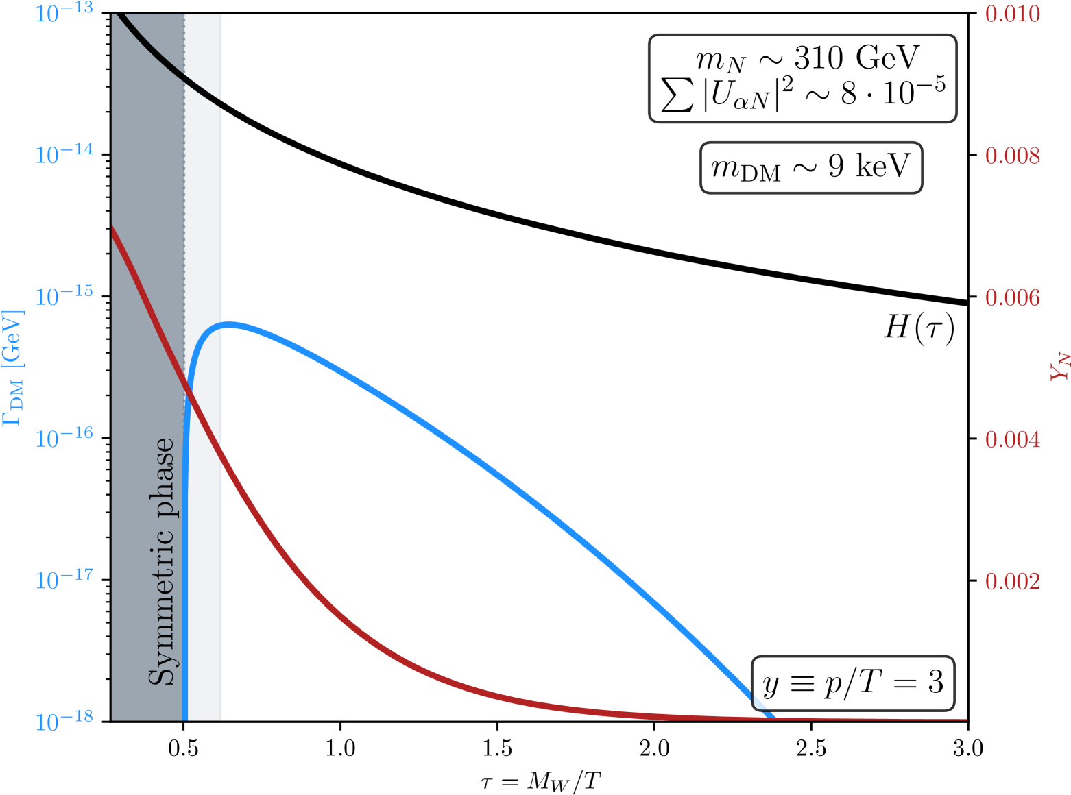
Figure 1: DM production rate (blue line) as a function of $\tau$ for $y=3$. The black line is the Hubble expansion rate, showing $\Gamma_{\mathrm{DM}}\ll H$, while the red one corresponds to the heavy pseudo-Dirac neutrino yield, $Y_{N}$. The dark gray area highlights the symmetric Higgs phase, while the light gray region corresponds to $\tau<\tau_{\mathrm{in}}$ (see Eq. (12)).

Once the DM distribution has frozen out, we can integrate its distribution over $y$ to find the number density. The fraction of DM produced compared to the observed one Aghanim et al. (2020) is then Lello and Boyanovsky (2016):

$$\begin{split}\mathcal{F}_{\mathrm{DM}}=&\left(\frac{\Omega_{\mathrm{DM}}^{\mathrm{obs}}h^{2}}{0.1198}\right)\frac{m_{\mathrm{DM}}}{7.4\,\mathrm{eV}}\frac{g_{\mathrm{DM}}}{g_{d}}\times\\ &\sum_{h=\pm 1}\int_{0}^{\infty}y^{2}dy\int_{\tau_{\mathrm{in}}}^{\tau_{\mathrm{fin}}}\frac{df^{h}_{\mathrm{DM}}}{d\tau}d\tau\,,\end{split}$$ (12)

where $g_{\mathrm{DM}}$ and $g_{d}\simeq 100$ are the DM degrees of freedom and the number of relativistic degrees of freedom at decoupling, respectively. In Eq. (12), the upper integration limit over $\tau$ corresponds to late enough times such that $\Gamma_{\mathrm{DM}}^{h}(\tau_{\mathrm{fin}})\rightarrow 0$. Instead, $\tau_{\mathrm{in}}$ corresponds to the time at which the DM production starts to be effective, which we take $\tau_{\mathrm{in}}\simeq 0.6>\tau_{\mathrm{SSB}}\equiv M_{W}/T_{\mathrm{SSB}}\simeq 0.5$.

Existing constraints: From the neutrino sector, we include the latest NuFIT results Esteban et al. (2024), allowing the mass-squared differences to vary in their 95 % CL ranges. Additionally, the size of the active-heavy mixing can be constrained with different experimental results depending on the heavy neutrino mass scale, $m_{N}$. For masses below the $Z$-boson mass, there are strong constraints from collider searches in which these heavy neutrinos can be produced Aad et al. (2019, 2023, 2024); Sirunyan et al. (2018); Tumasyan et al. (2022); Hayrapetyan et al. (2024a, b, c); Kelly and Machado (2021); Abratenko et al. (2024); Fernández-Mart´ınez et al. (2023). For larger masses, deviations from unitarity of the leptonic mixing matrix are the leading constraints. We include the bounds obtained at 95 % CL from a global fit to EWPO and cLFV in Ref. Blennow et al. (2023).

On the other hand, the active-DM mixing can be tightly constrained from indirect detection searches. This DM candidate decays radiatively into a photon and a light neutrino. For the DM masses in the $\mathcal{O}\left(1-100\right)$ keV range that we investigate, its decay produces a monochromatic X-ray signal Boyarsky et al. (2008); Roach et al. (2020); Foster et al. (2021); Roach et al. (2023), the non-observation of which constrains $\sin^{2}\theta_{\alpha\mathrm{DM}}\lesssim 10^{-11}$. Furthermore, light non-cold DM candidates such as sterile neutrinos can alter the primordial power spectrum with respect to the prediction of the standard $\Lambda$CDM model, leaving an imprint on the Ly-$\alpha$ forest Gnedin and Hamilton (2002); Boyarsky et al. (2009). However, these limits are model dependent as they rely on the DM distribution, which is in turn set by the particular production mechanism. Since we consider DM production from the decay of particles in thermal equilibrium, its distribution is related to a thermal one Petraki and Kusenko (2008); Ballesteros et al. (2021). We take the following lower bound on the DM mass Ballesteros et al. (2021):

$$m_{\rm DM}\geq 7.51\,\mbox{KeV}{\left(\frac{m_{\rm WDM}}{3\,\mbox{KeV}}\right)}^{4/3}{\left(\frac{106.75}{g_{d}}\right)}^{1/3}\,,$$ (13)

where $m_{\rm WDM}$ is the bound obtained on the DM mass from Ly-$\alpha$ for a warm dark matter (WDM) candidate Narayanan et al. (2000); Viel et al. (2005, 2013); Baur et al. (2016); Iršič et al. (2017); Palanque-Delabrouille et al. (2020); Garzilli et al. (2021). We will quote the bound using $m_{\mathrm{WDM}}=3$ keV, but we highlight that, given the uncertainties in the rescaling of the WDM limits, weaker constraints can be found using $m_{\mathrm{WDM}}\simeq 1.9$ keV Ballesteros et al. (2021).

Numerical analysis: We have computed $\Gamma_{\mathrm{DM}}^{h}$ over a lattice in $T$ and $p$, with $T\lesssim 130$ GeV, and integrated Eq. (11) to obtain the DM abundance today. The DM production rate is only different from zero after SSB, which in our analysis corresponds to $T_{\mathrm{SSB}}\sim 160$ GeV,as shown in Fig. 1. We explicitly include both the Higgs vev and mass temperature dependence in our study, while approximating gauge boson masses to their values at $T=0$ given that the Higgs vev becomes large soon after SSB.

Regarding the parameters in the neutrino sector, we scan over the whole range of the CP-violating phases entering in the PMNS mixing matrix, both Dirac and Majorana. Given that the DM candidate does not substantially contribute to light neutrino masses, the lightest neutrino is massless. The DM and heavy neutrino masses, as well as the complex angles parameterizing $R$ in Eq. (2), are varied over the ranges summarized in Table 1, where the parameter $\delta\vartheta_{12\,(13)}$ has a different definition depending on the mass ordering: $\delta\vartheta_{12\,(13)}=\vartheta_{12\,(13)}$ for NO or $\delta\vartheta_{12\,(13)}=\vartheta_{12\,(13)}\pm\pi/2$ for IO.

$|\delta\vartheta_{12\,(13)}|$	$\mathrm{Re}\vartheta_{23}$	$\mathrm{Im}\vartheta_{23}$	$m_{\mathrm{DM}}$ [keV]	$m_{N}$ [GeV]
$\left[10^{-7},\,10^{-2}\right]$	$\left[10^{-7},\,10^{-2}\right]$	$[5,\,20]$	$[5,\,100]$	$[10,\,10^{5}]$

Table 1: Parameter ranges for DM and heavy neutrino masses, and the complex angles parameterizing $R$ in Eq. (2). In order to have two almost degenerate heavy neutrinos we need $\vartheta_{12\,(13)}=\mp\pi/2+\delta\vartheta_{12\,(13)}$ for IO and $\vartheta_{12\,(13)}=\delta\vartheta_{12\,(13)}$ for NO, while $\mathrm{Im}\vartheta_{23}\gg 1$.

After checking the compatibility of a given set of parameters with oscillation data Esteban et al. (2024) and constraints from X-ray searches Boyarsky et al. (2008); Roach et al. (2020); Foster et al. (2021); Roach et al. (2023), we compute the DM abundance to obtain viable regions of parameter space accounting for the observed DM. These are then further constrained by Ly-$\alpha$ forest observations using Eq. (13), as well as bounds on the active-heavy mixings Blennow et al. (2023) which we parameterize by $\sum|U_{\alpha N}|^{2}\equiv\sum_{\alpha}\sum_{N=5,\,6}|U_{\alpha N}|^{2}$.

We present the results of our scan in Fig. 2. In the upper panel, we show the DM mixing as a function of its mass. The color code for the points (color bar on the right) corresponds to the generated DM fraction. The light blue area corresponds to current X-ray constraints Boyarsky et al. (2008); Roach et al. (2020); Foster et al. (2021); Roach et al. (2023) while the darker blue dash-dotted line shows the future sensitivity from XRISM Dessert et al. (2024). We show for illustration the region in which the Dodelson-Widrow (DW) mechanism produces all the DM Asaka et al. (2007) as a dotted black line, already ruled out. The gray shaded area corresponds to the bound on $m_{\mathrm{DM}}$ from Ly-$\alpha$. Noticeably, the total observed DM abundance can only be obtained for $m_{\mathrm{DM}}\lesssim 50\,\mathrm{keV}$. In the lower panel of Fig. 2 we show the dependence of the DM fraction on the size of the active-heavy mixing. In this case the color code represents the size of $\sin^{2}{\theta_{\alpha\mathrm{DM}}}$. The red horizontal line sets $\mathcal{F}_{\mathrm{DM}}=1$, while gray squared points correspond to regions of parameter space ruled out by Ly-$\alpha$. Although any region above the red line overcloses the Universe and is effectively ruled out, we show it to better understand the dependence on $\sum|U_{\alpha N}|^{2}$. The gray shaded area corresponds to the bound on $\sum|U_{\alpha N}|^{2}$ from EWPO and cLFV for NO Blennow et al. (2023). While it is obvious that larger Yukawa couplings translate into a larger DM abundance, we note from this plot that the whole parameter space can be probed with future experiments. On the one hand, constraints pertaining the DM such as X-ray searches or Ly-$\alpha$ tend to close the allowed parameter space over the diagonal. On the other hand, bounds from EWPO and cLFV on $\sum|U_{\alpha N}|^{2}$ shut the parameter space in a complementary direction. Similar conclusions are found for the IO case and we do not show the corresponding plots.

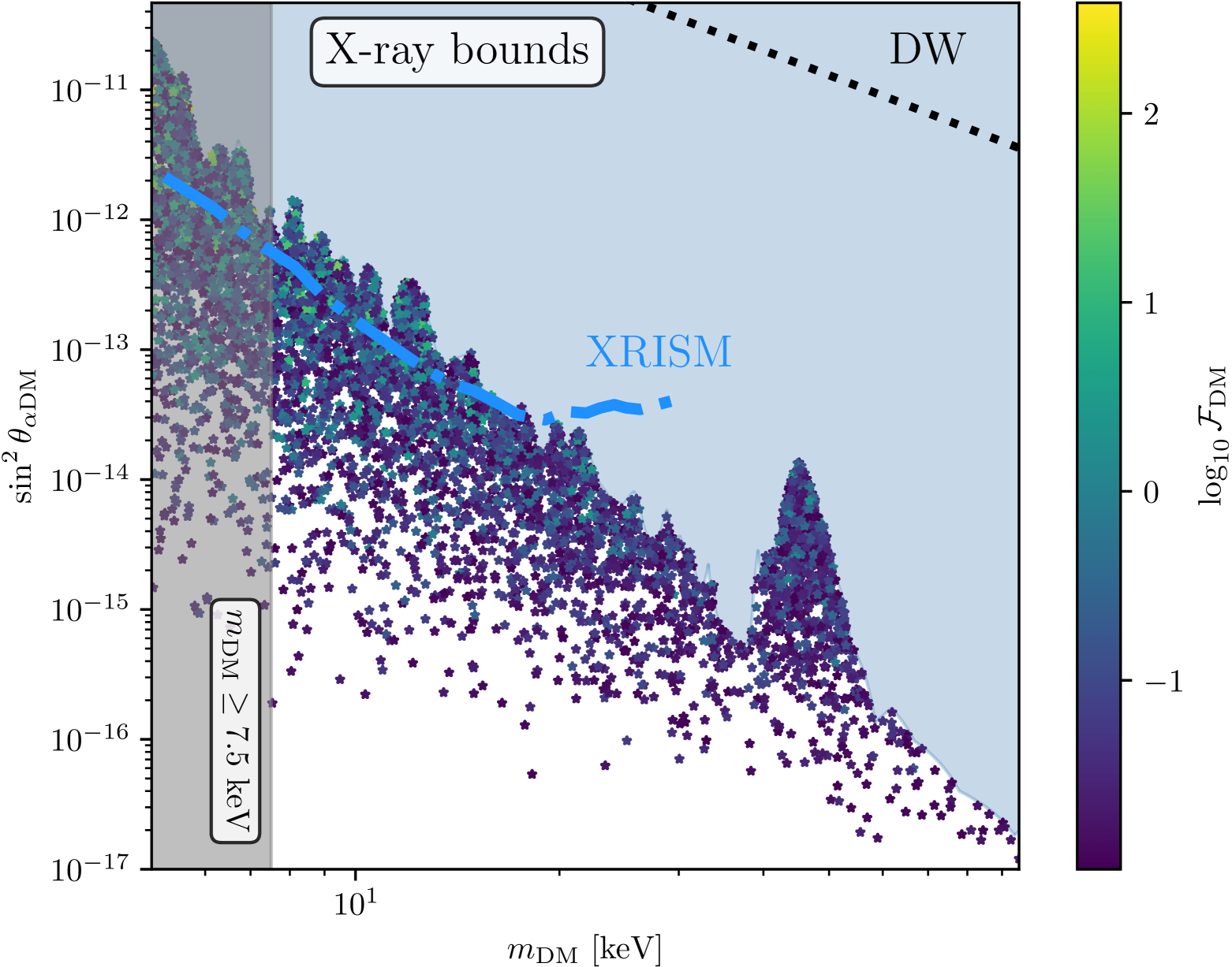
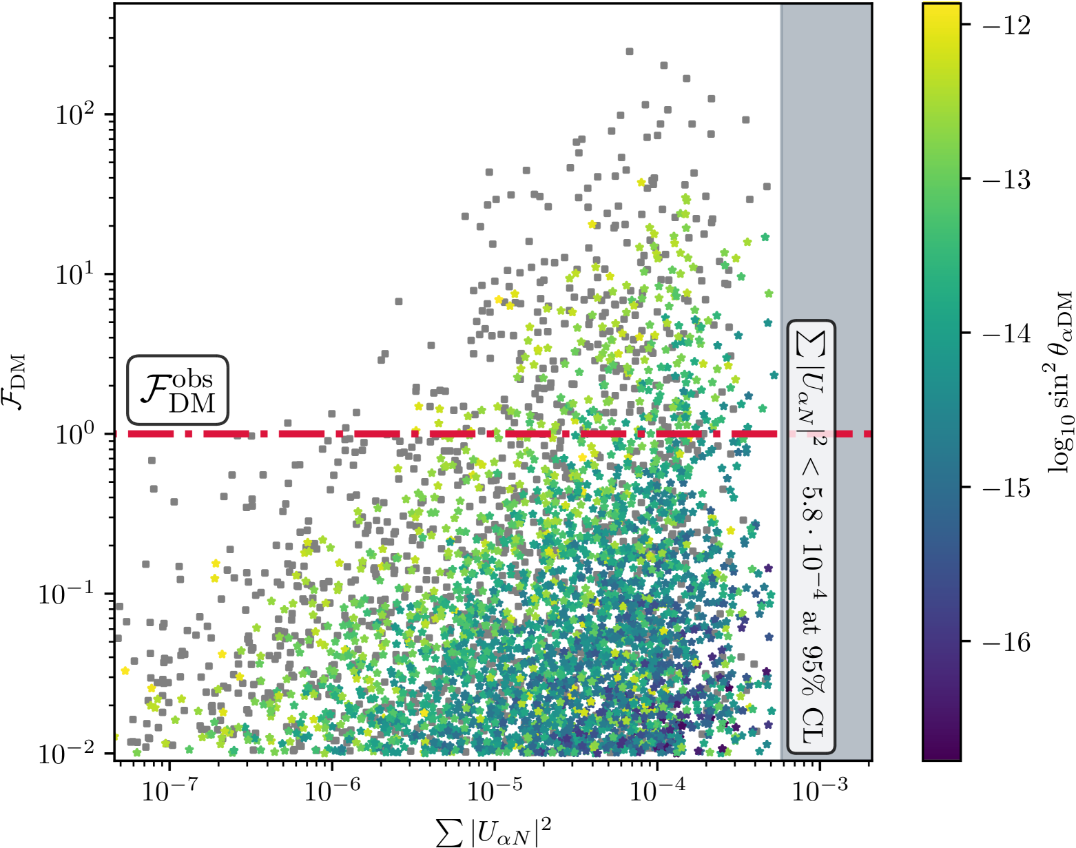
Figure 2: Results for regions of parameter space producing at least $1$ % of the observed DM for NO. The upper panel shows the results on the DM mixing vs DM mass plane, with the color bar representing the DM fraction. The lower panel shows the DM fraction as a function of the active-heavy mixing. The DM mixing is shown in the corresponding color bar. Relevant experimental and observational bounds are shown in each slice of parameter space (see text for details).

Future machines like FCC-ee aim to improve current measurements of EWPO reducing uncertainties by at least one order of magnitude Abada et al. (2019), while the quest to find cLFV is still ongoing with the notable example of MEG-II Baldini et al. (2018, 2021); Afanaciev et al. (2024), searching for $\mu\rightarrow e\gamma$ and currently running. We show in the upper panel of Fig. 3 the consequences large $\sum|U_{\alpha N}|^{2}$ has on the invisible decay width of the $Z$-boson $\Gamma_{\mathrm{inv}}^{Z}$, and on $\mathcal{B}\left(\mu\rightarrow e\gamma\right)$, after taking into account existing constraints. The color code (in both panels) represents once again the DM abundance for each point, with $10^{-1}\lesssim\mathcal{F}_{\mathrm{DM}}\lesssim 5$. The orange dash-dotted line represents the potential lower $1\sigma$ region on $\Gamma_{\mathrm{inv}}^{Z}$ assuming the SM central value and the reduction of current uncertainties by one order of magnitude Navas et al. (2024); Abada et al. (2019). Furthermore, we show the prospects from MEG-II Baldini et al. (2021) with the blue dashed vertical line.

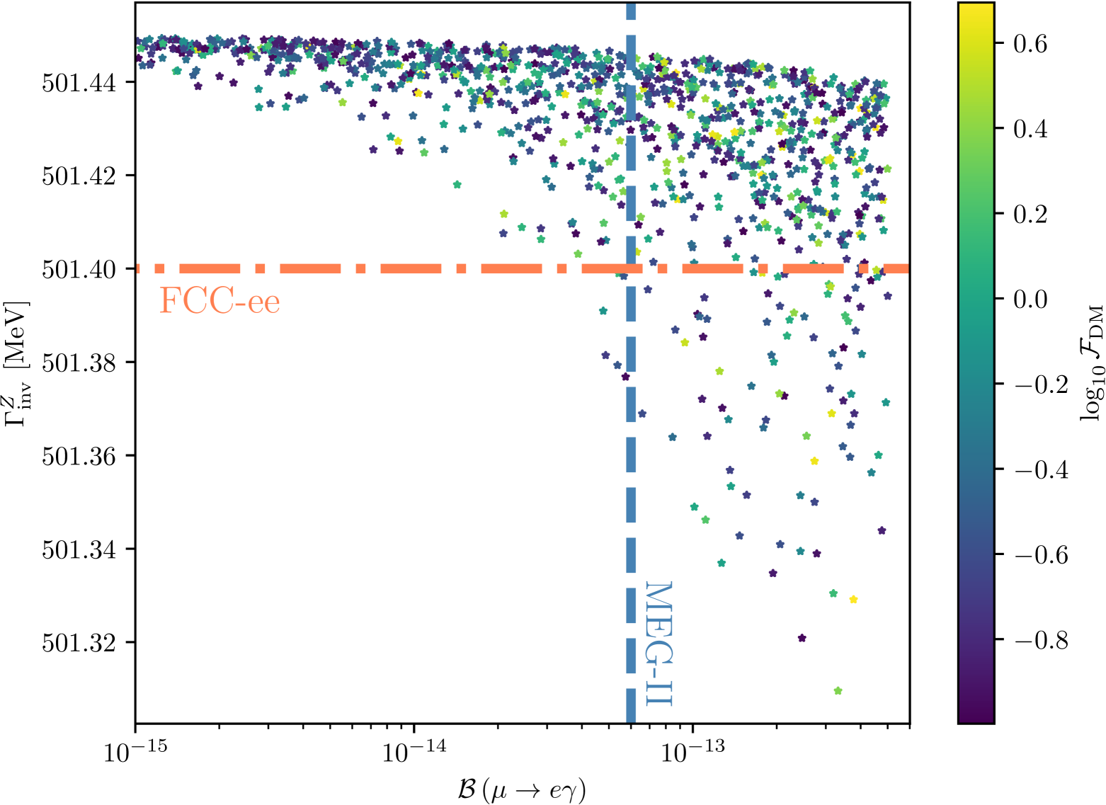
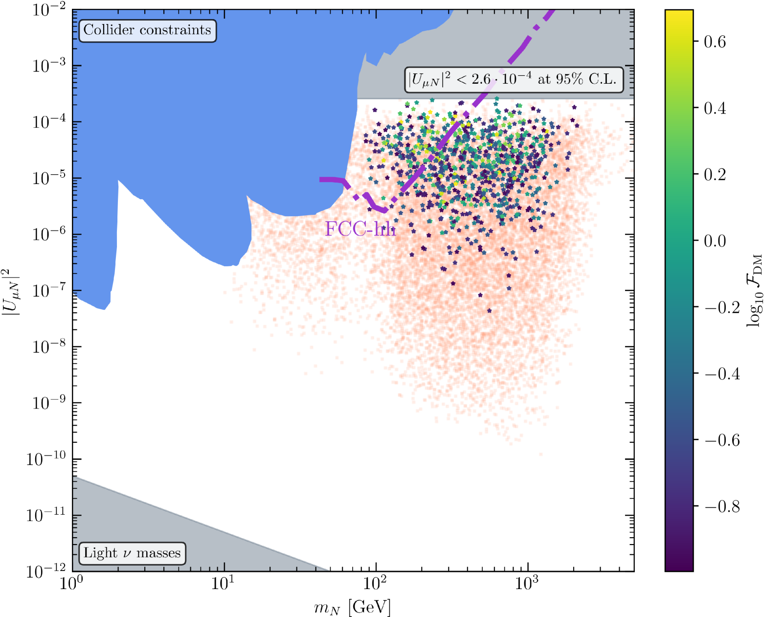
Figure 3: Prospects to probe the parameter space generating $10^{-1}\lesssim\mathcal{F}_{\mathrm{DM}}\lesssim 5$. In the upper panel we show correlations between the invisible decay width of the $Z$-boson and searches for $\mu\rightarrow e\gamma$, together with prospective sensitivities for FCC-ee and MEG-II. In the lower panel we present the relevant parameter space for the active-heavy mixing $|U_{\mu N}|^{2}$ and $m_{N}$ including relevant experimental bounds Fernández-Mart´ınez et al. (2023); Blennow et al. (2023). The purple line corresponds to the sensitivity of FCC-hh Abdullahi et al. (2023).

Finally, we show in the lower panel of Fig. 3 our results as a function of the heavy pseudo-Dirac pair mass and their mixing with the muon-neutrino flavor for NO. The shaded blue area corresponds to current collider bounds at $90$ % CL, obtained using HNLimits Fernández-Mart´ınez et al. (2023). The gray horizontal region corresponds to the bounds on $|U_{\mu N}|^{2}$ from EWPO and cLFV Blennow et al. (2023) while the lower gray area corresponds to the naive lower bound on $|U_{\mu N}|^{2}$ for which the observed mass-squared differences Esteban et al. (2020) are generated. The light red cloud of points shows regions of parameter space for which the produced DM abundance is too small ($10^{-5}\lesssim\mathcal{F}_{\mathrm{DM}}\lesssim 10^{-1}$). In order to produce a non-negligible DM abundance we find $100\,\mathrm{GeV}\lesssim m_{N}\lesssim 1\,\mathrm{TeV}$. Since production is only possible for $T\lesssim 160$ GeV, the DM abundance is exponentially suppressed for $m_{N}\gtrsim 1\,\mathrm{TeV}$ due to the Boltzmann suppression of the heavy neutrino distribution. Prospects from FCC-hh Abdullahi et al. (2023) are shown as a dash-dotted purple line, covering relevant regions of parameter space for $m_{N}\lesssim 300$ GeV.

Conclusions: In this letter we proposed a combined solution for the neutrino masses and DM puzzles based on a minimal low-scale seesaw framework, which might also be compatible with leptogenesis. DM production is accounted for through two-body decays of SM bosons, as well as decays of the heavy neutrinos involving DM and a SM boson, at temperatures below the electroweak crossover. For the first time, we perform a complete computation, based on the evaluation of neutrino self-energies in the context of TFT, consistently accounting for all the available production channels, and analyze the phenomenological consequences of such a scenario.

In order for the production to be efficient, approximate lepton number conservation is necessary. This translates into a heavy neutrino spectrum comprised by the DM candidate, with mass $\mathcal{O}\left(10\right)$ keV and almost decoupled, and two heavy Majorana neutrinos with almost degenerate masses, $m_{N}$, and large mixings with the active ones. We find that the heavy neutrino decay into the DM candidate dominates its production, which translates into the rough upper bound $m_{N}\lesssim 1$ TeV. Above these masses, the heavy neutrinos would not be abundant enough in the thermal plasma after SSB and the generation of mixings.

The phenomenological implications of such a DM production mechanism are very rich, as it introduces strong synergies between the expected signal in the usual indirect DM probes, such as X-ray searches or constraints from structure formation, and the size of the active-heavy neutrino mixings controlling the final DM abundance. Indeed, current EWPO and searches for cLFV place the leading constraints on this scenario. We find that MEG-II, currently taking data, will be able to probe part of the parameter space for which all the observed DM is generated. In the longer term, the simultaneous improvement of indirect DM searches with experiments like XRISM, as well as the measurement of EWPO in FCC-ee together with searches for cLFV (or even direct searches in FCC-hh) has the potential to completely test this DM generation mechanism.

Acknowledgments: S. R. A sincerely thanks E. Fernandez-Martinez for insightful discussions on the non-unitarity bounds of the leptonic mixing matrix. He also appreciates J. Hernandez-Garcia’s assistance with HNLimits and stimulating exchanges with P. Hernandez and N. Rius. Special thanks to Alessandro Granelli for comments on the lepton number conserving limit of the Casas-Ibarra parameterization. M. L. thanks Fermilab for hosting him during the development of this work. M. L. is funded by the European Union under the Horizon Europe’s Marie Sklodowska-Curie project 101068791 — NuBridge. A.A. acknowledges support from the European Union’s Horizon 2020 research and innovation programme under the Marie Skłodowska -Curie grant agreement No 860881-HIDDeN and the Marie Skłodowska-Curie Staff Exchange grant agreement No 101086085 – ASYMMETRY.

¹Pôle Théorie, Laboratoire de Physique des 2 Infinis Irène Joliot Curie (UMR 9012),

CNRS/IN2P3, 15 Rue Georges Clemenceau, 91400 Orsay, France

² Dipartimento di Scienze Matematiche e Informatiche, Scienze Fisiche e Scienze della Terra,

Università degli Studi di Messina, Viale Ferdinando Stagno d’Alcontres 31, I-98166 Messina, Italy

³ INFN Sezione di Catania, Via Santa Sofia 64, I-95123 Catania, Italy

⁴ Dipartimento di Fisica e Astronomia, Università di Bologna, via Irnerio 46, 40126 Bologna, Italy

⁵ INFN, Sezione di Bologna, viale Berti Pichat 6/2, 40127 Bologna, Italy

Appendix A Neutrino self-energy corrections

In this section we specify, for completeness, the lagrangian describing the interactions between massive neutrinos and the SM bosons after SSB as well as the diagrams contributing to the neutrino self-energies. We can write the relation between the active neutrinos $\nu_{\alpha L}$, and the mass neutrino eigenstates $n_{i}$ (with masses $m_{i}$), as

$$\begin{split}\nu_{L,\,\alpha}=\sum_{i=1}^{6}U_{\alpha i}P_{L}n_{i}\,\end{split}$$ (14)

where $\alpha=e,\,\mu,\,\tau$ and $i=1,\,2,\,3$ corresponds to light neutrinos while $i=4,\,5,\,6$ to the heavy mostly-sterile ones. Rewriting the interaction lagrangian in the mass basis, taking into account that $n_{i}$ are Majorana states, we find

$$\begin{split}\mathcal{L}_{W-n}\supset&\frac{g}{\sqrt{2}}W_{\mu}\sum_{i=1}^{6}\sum_{\alpha}U_{\alpha i}\bar{\ell}_{\alpha}\gamma^{\mu}P_{L}n_{i}+h.c.\,,\\ \mathcal{L}_{Z-n}\supset&\frac{g}{4c_{W}}Z_{\mu}\sum_{i,j=1}^{6}\bar{n}_{i}\big{[}C_{ij}\gamma^{\mu}P_{L}-C_{ij}^{*}\gamma^{\mu}P_{R}\big{]}n_{j}\,,\\ \mathcal{L}_{h-n}\supset&-\frac{1}{2v_{H}}h\sum_{i,j=1}^{6}\bar{n}_{i}\big{[}C_{ij}\left(m_{i}P_{L}+m_{j}P_{R}\right)+C^{*}_{ij}\left(m_{i}P_{R}+m_{j}P_{L}\right)\big{]}n_{j}\,,\end{split}$$ (15)

where $\ell_{\alpha}$ are the charged lepton fields, $C_{ij}\equiv\sum_{\alpha}U_{i\alpha}^{\dagger}U_{\alpha j}$, $v_{H}$ is the Higgs vev, $g$ the $SU(2)_{L}$ gauge coupling and $c_{W}$ is a short-hand notation for the cosine of the weak mixing angle. Given these interaction terms, the neutrino self-energy corrections are given by the diagrams in Fig. 4 involving a Higgs or a gauge boson. Following Ref. Weldon (1983), one can relate these self-energy corrections to the different decays we are interested in, namely $n_{k}\rightarrow h\,(Z)+\mathrm{DM}$ with $m_{k}\gtrsim M_{H}\,(M_{Z})$, $h\,(Z)\rightarrow n_{k}+\mathrm{DM}$ with $n_{k}$ a light mostly-active neutrino (or a heavy mostly-sterile one with $m_{k}<M_{H}\,(M_{Z})$), and $W\rightarrow\ell_{\alpha}+\mathrm{DM}$.

Figure 4: Feynman diagrams contributing to the neutrino self-energy. In the SM extension with singlet fermions, there is the Higgs contribution (left) and the gauge contribution from the $W$ and $Z$ bosons (right). The imaginary part of the self-energy is related to the rate at which each species approaches equilibrium.

Appendix B Derivation of the DM production rate

The computation of the DM production rate follows an analogous strategy to Refs. Lello et al. (2017); Abada et al. (2023). We can decompose the neutrino self-energy corrections depicted in Fig. 4 as

$$\not{\Sigma}^{\chi}=\gamma_{0}\Sigma^{\chi\,(0)}-\vec{\gamma}\cdot\hat{p}\Sigma^{\chi\,(1)}+\Sigma^{\chi\,(2)}\,,$$ (16)

where each $\Sigma^{\chi\,(i)}$ depends on $p^{\mu}$ and $T$. Such self-energy corrections have been determined in Abada et al. (2023) using the real time formalism of TFT Schwinger (1961); Keldysh (1964); Le Bellac (1996); Kapusta and Gale (2006); Lundberg and Pasechnik (2021), to which the reader can refer for more details. Projecting the equation of motion with $P_{L,R}=\left(1\mp\gamma_{5}\right)/2$ and expanding the fields in helicity eigenstates:

$$\psi_{\chi}=\sum_{h=\pm 1}v^{h}\otimes\psi_{\chi}^{h},$$ (17)

with $v^{h}$ being the eigenstates of the helicity operator with $h=\pm 1$ and $\chi\in\{L,\,R\}$, one arrives at the full inverse propagator in the medium:

$$\begin{split}\mathcal{S}^{-1}_{h}\equiv&p_{0}^{2}-p^{2}-\Omega_{h}=p_{0}^{2}-p^{2}+\left(p_{0}-hp\right)\left(\Sigma^{L\,(0)}+h\Sigma^{L\,(1)}\right)\\ &-\left(p_{0}-hp\right)\left(\mathcal{M}+\Sigma^{R\,(2)}\right)\left[p_{0}-hp+\Sigma^{R\,(0)}-h\Sigma^{R\,(1)}\right]^{-1}\left(\mathcal{M}+\Sigma^{L\,(2)}\right)\,.\end{split}$$ (18)

Note that this is a matrix equation in “flavor” space, such as $p_{0}$ and $p$ are proportional to the identity matrix, which is not explicitly written. In order to find the propagating states in the medium, one needs to find the simple poles of the propagator, or rather the complex zeroes of its inverse given in Eq. (18). The imaginary part of the complex zeros of $\mathcal{S}_{h}^{-1}$ for each propagating neutrino species will be related to the rate at which they reach equilibrium Weldon (1983).

The first step to obtain $\Gamma_{\mathrm{DM}}^{h}$ is to find the eigenvalue of $\Omega_{h}$ associated to the DM candidate, which we call $\omega_{h}$, such that we can obtain the dispersion relation of the DM in the medium as $p_{0}^{2}-p^{2}-\omega_{h}=0$. We expect it to behave as $\omega_{h}\sim m_{\mathrm{DM}}^{2}+\delta\omega_{h}$ with $|\delta\omega_{h}|\ll m_{\mathrm{DM}}^{2}$. To this purpose, we separate $\Omega_{h}$ into blocks corresponding to the light mostly-active neutrino species (denoted with indexes $l,\,l^{\prime}=1,\,2,\,3$) and the heavy mostly-sterile ones (denoted by $h,\,h^{\prime}=4,\,5,\,6$):

$$\Omega\equiv\begin{pmatrix}\Omega_{ll^{\prime}}&\Omega_{lh^{\prime}}\\ \Omega_{hl^{\prime}}&\Omega_{hh^{\prime}}\end{pmatrix}\,.$$ (19)

We further define $\Sigma^{L}\equiv\Sigma^{L\,(0)}+h\Sigma^{L\,(1)}$ and $\Sigma^{R}\equiv\Sigma^{R\,(0)}-h\Sigma^{R\,(1)}$, whose explicit expressions in therms of the neutrino mixings and couplings are

$$\begin{split}\left(\Sigma^{R}\right)_{ij}=&\frac{1}{4}\sum_{k=1}^{6}\left\{\left(\frac{g}{2c_{W}}\right)^{2}C_{ik}^{*}(\sigma^{(0)}_{k,\,Z}-h\sigma^{(1)}_{k,\,Z})C^{*}_{kj}+\frac{1}{v_{H}^{2}}\left(C^{*}_{ik}m_{i}+C_{ik}m_{k}\right)(\sigma^{(0)}_{k,\,H}-h\sigma^{(1)}_{k,H})\left(C_{kj}m_{j}+C^{*}_{kj}m_{k}\right)\right\}\,,\\ \left(\Sigma^{L}\right)_{ij}=&\frac{g^{2}}{2}C_{ij}(\sigma^{(0)}_{W}+h\sigma^{(1)}_{W})\\ +&\frac{1}{4}\sum_{k=1}^{6}\left\{\left(\frac{g}{2c_{W}}\right)^{2}C_{ik}(\sigma^{(0)}_{k,\,Z}+h\sigma^{(1)}_{k,\,Z})C_{kj}+\frac{1}{v_{H}^{2}}\left(C_{ik}m_{i}+C^{*}_{ik}m_{k}\right)(\sigma^{(0)}_{k,\,H}+h\sigma^{(1)}_{k,H})\left(C^{*}_{kj}m_{j}+C_{kj}m_{k}\right)\right\}\,.\end{split}$$ (20)

In Eq. (20), $\sigma_{k,\,B}^{(i)}$ is the thermal part of the amplitude for the $k^{\mathrm{th}}$-neutrino mass eigenstate and $B$ corresponds to either the Higgs or Z-boson. For the $W$-boson contribution, $\sigma_{W}^{(i)}$, we neglect charged lepton masses. The superscript $(i)$ labels the different projections of the self-energy from Eq. (16). Details on the computation of these thermal parts can be found in Ref. Abada et al. (2023). Using Eq. (9) and neglecting light neutrino masses we find that the dominant contributions to $\Omega$ are given by

$$\Omega=-\left(p_{0}-hp\right)\begin{pmatrix}\Sigma^{L}_{ll^{\prime}}&\Sigma^{L}_{lh^{\prime}}-\Sigma^{R\,(2)}_{lh^{\prime}}P_{h^{\prime}h}^{R}M_{\mathrm{heavy}}\\ \Sigma^{L}_{hl^{\prime}}-M_{\mathrm{heavy}}P_{h^{\prime}h}^{R}\Sigma^{L\,(2)}_{hl^{\prime}}&\Sigma^{L}_{hh^{\prime}}-M_{\mathrm{heavy}}P_{h^{\prime}h}^{R}M_{\mathrm{heavy}}\end{pmatrix}\,,$$ (21)

with $P_{h^{\prime}h}^{R}\equiv\left[p_{0}-hp+\Sigma^{R}_{hh^{\prime}}-\Sigma^{R}_{hl^{\prime}}\left(p_{0}-hp+\Sigma^{R}_{ll^{\prime}}\right)^{-1}\Sigma^{R}_{lh^{\prime}}\right]^{-1}$ and $M_{\mathrm{heavy}}\simeq\mathrm{diag}(m_{\mathrm{DM}},\,m_{N},\,m_{N})$. At this point, we need to specify the helicity in order to do further simplifications.

• Positive helicity $h=+1$:

  We can approximate $p_{0}-hp\simeq m_{\mathrm{DM}}^{2}/(2p)$ for the DM candidate, finding as well that $P_{h^{\prime}h}^{R}\simeq\mathcal{P}^{R}$ as defined in the main text. Terms proportional to $M_{\mathrm{heavy}}$ dominate and thus we have to solve the following eigenvalue problem

  $$\mathrm{det}\begin{pmatrix}-\frac{m_{\mathrm{DM}}^{2}}{2p}\Sigma^{L}_{ll^{\prime}}-\omega_{+1}&\frac{m_{\mathrm{DM}}^{2}}{2p}\Sigma^{R\,(2)}_{lh^{\prime}}\mathcal{P}^{R}M_{\mathrm{heavy}}\\ \frac{m_{\mathrm{DM}}^{2}}{2p}M_{\mathrm{heavy}}\mathcal{P}^{R}\Sigma^{L\,(2)}_{hl^{\prime}}&\frac{m_{\mathrm{DM}}^{2}}{2p}M_{\mathrm{heavy}}\mathcal{P}^{R}M_{\mathrm{heavy}}-\omega_{+1}\end{pmatrix}=0\,.$$ (22)

  Using the fact that $\omega_{+1}\sim m_{\mathrm{DM}}^{2}+\delta\omega_{+1}$, with $|\delta\omega_{+1}|/m_{\mathrm{DM}}^{2}\ll 1$, we can compute the determinant by blocks and focus on the dominant term which is given by

  $$\mathrm{det}\Bigg{[}\frac{m_{\mathrm{DM}}^{2}}{2p}M_{\mathrm{heavy}}\mathcal{P}^{R}M_{\mathrm{heavy}}-\omega_{+1}\Bigg{]}=0\,,$$ (23)

  where we have dropped terms of order $\mathcal{O}\left(m_{\mathrm{DM}}^{2}/p^{2}\right)$. Computing the determinant in Eq. (23) by further dividing the heavy sector into the DM and the heavy pseudo-Dirac pair blocks, we arrive at the rate given in Eq. (5) in the main text by using the relation $\Gamma^{h=+1}_{\mathrm{DM}}=-2\mathrm{Im}\left[\sqrt{p^{2}+\omega_{+1}}\right]$.

• Negative helicity $h=-1$:

  For negative helicity DM we have $p_{0}-hp\simeq 2p$, and thus the eigenvalue problem we need to solve is instead

  $$\mathrm{det}\begin{pmatrix}-2p\Sigma^{L}_{ll^{\prime}}-\omega_{-1}&-2p\Sigma^{L}_{lh^{\prime}}\\ -2p\Sigma^{L}_{hl^{\prime}}&-2p\left(\Sigma^{L}_{hh^{\prime}}-M_{\mathrm{heavy}}P^{R}_{h^{\prime}h}M_{\mathrm{heavy}}\right)-\omega_{-1}\end{pmatrix}=0\,.$$ (24)

  In this case, we can approximate $P^{R}_{h^{\prime}h}\simeq\left(\mathbb{I}_{3}-\Sigma^{R}_{h^{\prime}h}/(2p)\right)/(2p)$, such that we need to solve

  $$\mathrm{det}\Big{[}-2p\left(\Sigma^{L}_{hh^{\prime}}-M_{\mathrm{heavy}}P^{R}_{h^{\prime}h}M_{\mathrm{heavy}}\right)-\omega_{-1}+4p^{2}\Sigma^{L}_{hl^{\prime}}\left[2p\Sigma^{L}_{ll^{\prime}}+\omega_{-1}\right]^{-1}\Sigma^{L}_{lh^{\prime}}\Big{]}=0\,.$$ (25)

  Making use of the fact that $2p\Sigma_{ll^{\prime}}^{L}\gg m_{\mathrm{DM}}^{2}$ and neglecting terms suppressed by powers of the momentum, while further dividing between the DM and heavy pseudo-Dirac pair blocks, we arrive at the production rate given in Eq. (6) of the main text by using the the fact that $\Gamma^{h=-1}_{\mathrm{DM}}=-2\mathrm{Im}\left[\sqrt{p^{2}+\omega_{-1}}\right]$.

Appendix C EW symmetry breaking

In order to follow the evolution of EW symmetry breaking as well as the temperature dependence of the Higgs vev and its mass it is necessary to study the Higgs effective potential at finite temperature. Lattice simulations show that the EW crossover starts at $T_{\mathrm{SSB}}\sim 160$ GeV and that the Higgs vev approaches its zero temperature value soon after D’Onofrio et al. (2014). We study the temperature evolution of the Higgs vev and its mass by analyzing the one-loop effective potential including temperature corrections Quiros (1999):

$$V(\langle h\rangle,T)=2D(T^{2}-T_{0}^{2})\langle h\rangle^{2}-ET\langle h\rangle^{3}+\frac{\lambda}{4}\langle h\rangle^{4}\,.$$ (26)

We explicitly written the potential in Eq. (26) in terms of the background field $\langle h\rangle$, and the constants $D$, $T_{0}^{2}$, and $E$ can be found in Ref. Quiros (1999) in terms of the physical masses of the gauge bosons and the top quark. In particular, $T_{0}^{2}$ sets the temperature at which SSB happens and we set its value to $T_{0}\sim 160$ GeV, in agreement with lattice results D’Onofrio et al. (2014). Compared to Ref. Quiros (1999), we neglect the temperature corrections in the Higgs quartic coupling given that they largely simplify our analysis while introducing a negligible change.

For $T<T_{0}$, the Higgs develops a vev, $\langle h\rangle=v(T)$, given by

$$\begin{split}v(T)=\frac{3ET+\sqrt{9E^{2}T^{2}-16D\lambda(T^{2}-T_{0}^{2})}}{2\lambda}\,,\end{split}$$ (27)

while its mass is found to be

$$M_{H}^{2}(T)\equiv\frac{\partial^{2}V(\langle h\rangle,T)}{\partial\langle h\rangle^{2}}\Bigg{|}_{\langle h\rangle=v(T)}=4D(T^{2}-T_{0}^{2})-6ETv(T)+3\lambda v(T)^{2}\,.$$ (28)

We show in Fig. 5 the temperature evolution of the Higgs vev (left panel) and its mass (blue line in right panel), which are fully taken into account in our analysis. We also show for illustration the gauge boson mass temperature dependence, which is proportional to the Higgs vev. Note however that the gauge boson thermal masses are not included here. The gray region represents the temperatures above which we do not compute the DM production to avoid a strong dependence on the dynamics of the crossover near the critical temperature.

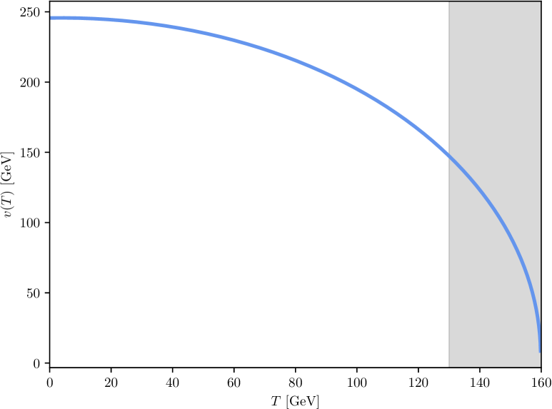
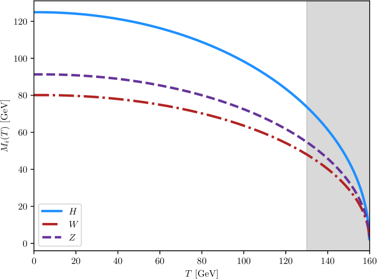
Figure 5: Temperature evolution of the Higgs vev given by Eq. (27) (left panel) and the temperature dependent Higgs mass including the leading thermal corrections (right panel). Additionally, we show the evolution of the gauge boson masses which are proportional to the Higgs vev. The gray shaded area corresponds to temperatures $T\gtrsim 130$ GeV for which we do not compute the DM production.

References

- Fukugita and Yanagida (1986) M. Fukugita and T. Yanagida, Phys. Lett. B174, 45 (1986).
- Akhmedov et al. (1998) E. K. Akhmedov, V. A. Rubakov, and A. Yu. Smirnov, Phys. Rev. Lett. 81, 1359 (1998), arXiv:hep-ph/9803255 [hep-ph] .
- Davidson et al. (2008) S. Davidson, E. Nardi, and Y. Nir, Phys. Rept. 466, 105 (2008), arXiv:0802.2962 [hep-ph] .
- Hernández et al. (2016) P. Hernández, M. Kekic, J. López-Pavón, J. Racker, and J. Salvado, JHEP 08, 157 (2016), arXiv:1606.06719 [hep-ph] .
- Abada et al. (2017) A. Abada, G. Arcadi, V. Domcke, and M. Lucente, JCAP 12, 024 (2017), arXiv:1709.00415 [hep-ph] .
- Sandner et al. (2023) S. Sandner, P. Hernandez, J. Lopez-Pavon, and N. Rius, JHEP 11, 153 (2023), arXiv:2305.14427 [hep-ph] .
- Asaka et al. (2005) T. Asaka, S. Blanchet, and M. Shaposhnikov, Phys. Lett. B 631, 151 (2005), arXiv:hep-ph/0503065 .
- Asaka and Shaposhnikov (2005) T. Asaka and M. Shaposhnikov, Phys. Lett. B620, 17 (2005), arXiv:hep-ph/0505013 [hep-ph] .
- Asaka et al. (2007) T. Asaka, M. Laine, and M. Shaposhnikov, JHEP 01, 091 (2007), [Erratum: JHEP 02, 028 (2015)], arXiv:hep-ph/0612182 .
- Shaposhnikov (2008) M. Shaposhnikov, JHEP 08, 008 (2008), arXiv:0804.4542 [hep-ph] .
- Laine and Shaposhnikov (2008) M. Laine and M. Shaposhnikov, JCAP 06, 031 (2008), arXiv:0804.4543 [hep-ph] .
- Canetti et al. (2013) L. Canetti, M. Drewes, T. Frossard, and M. Shaposhnikov, Phys. Rev. D 87, 093006 (2013), arXiv:1208.4607 [hep-ph] .
- Ghiglieri and Laine (2019) J. Ghiglieri and M. Laine, JHEP 07, 078 (2019), arXiv:1905.08814 [hep-ph] .
- Ghiglieri and Laine (2020) J. Ghiglieri and M. Laine, JCAP 07, 012 (2020), arXiv:2004.10766 [hep-ph] .
- Minkowski (1977) P. Minkowski, Phys. Lett. 67B, 421 (1977).
- Mohapatra and Senjanovic (1980) R. N. Mohapatra and G. Senjanovic, Phys. Rev. Lett. 44, 912 (1980), [,231(1979)].
- Yanagida (1979) T. Yanagida, Proceedings: Workshop on the Unified Theories and the Baryon Number in the Universe: Tsukuba, Japan, February 13-14, 1979, Conf. Proc. C7902131, 95 (1979).
- Gell-Mann et al. (1979) M. Gell-Mann, P. Ramond, and R. Slansky, Conf. Proc. C 790927, 315 (1979), arXiv:1306.4669 [hep-th] .
- Esteban et al. (2024) I. Esteban, M. C. Gonzalez-Garcia, M. Maltoni, I. Martinez-Soler, J. a. P. Pinheiro, and T. Schwetz, JHEP 12, 216 (2024), arXiv:2410.05380 [hep-ph] .
- Branco et al. (1989) G. C. Branco, W. Grimus, and L. Lavoura, Nucl. Phys. B312, 492 (1989).
- Kersten and Smirnov (2007) J. Kersten and A. Yu. Smirnov, Phys. Rev. D76, 073005 (2007), arXiv:0705.3221 [hep-ph] .
- Abada et al. (2007) A. Abada, C. Biggio, F. Bonnet, M. B. Gavela, and T. Hambye, JHEP 12, 061 (2007), arXiv:0707.4058 [hep-ph] .
- Moffat et al. (2017) K. Moffat, S. Pascoli, and C. Weiland, (2017), arXiv:1712.07611 [hep-ph] .
- Lucente (2023) M. Lucente, Phys. Lett. B 846, 138206 (2023), arXiv:2103.03253 [hep-ph] .
- Schechter and Valle (1980) J. Schechter and J. W. F. Valle, Phys. Rev. D 22, 2227 (1980).
- Gronau et al. (1984) M. Gronau, C. N. Leung, and J. L. Rosner, Phys. Rev. D 29, 2539 (1984).
- Malinsky et al. (2005) M. Malinsky, J. C. Romao, and J. W. F. Valle, Phys. Rev. Lett. 95, 161801 (2005), arXiv:hep-ph/0506296 [hep-ph] .
- Abada and Lucente (2014) A. Abada and M. Lucente, Nucl. Phys. B 885, 651 (2014), arXiv:1401.1507 [hep-ph] .
- Abada et al. (2014) A. Abada, G. Arcadi, and M. Lucente, JCAP 10, 001 (2014), arXiv:1406.6556 [hep-ph] .
- Mohapatra (1986) R. N. Mohapatra, Phys. Rev. Lett. 56, 561 (1986).
- Mohapatra and Valle (1986) R. N. Mohapatra and J. W. F. Valle, Sixty years of double beta decay: From nuclear physics to beyond standard model particle physics, Phys. Rev. D34, 1642 (1986), [,235(1986)].
- Barr (2004) S. M. Barr, Phys. Rev. Lett. 92, 101601 (2004), arXiv:hep-ph/0309152 .
- Shaposhnikov (2007) M. Shaposhnikov, Nucl. Phys. B 763, 49 (2007), arXiv:hep-ph/0605047 .
- Boyarsky et al. (2008) A. Boyarsky, D. Malyshev, A. Neronov, and O. Ruchayskiy, Mon. Not. Roy. Astron. Soc. 387, 1345 (2008), arXiv:0710.4922 [astro-ph] .
- Roach et al. (2020) B. M. Roach, K. C. Y. Ng, K. Perez, J. F. Beacom, S. Horiuchi, R. Krivonos, and D. R. Wik, Phys. Rev. D 101, 103011 (2020), arXiv:1908.09037 [astro-ph.HE] .
- Foster et al. (2021) J. W. Foster, M. Kongsore, C. Dessert, Y. Park, N. L. Rodd, K. Cranmer, and B. R. Safdi, Phys. Rev. Lett. 127, 051101 (2021), arXiv:2102.02207 [astro-ph.CO] .
- Roach et al. (2023) B. M. Roach, S. Rossland, K. C. Y. Ng, K. Perez, J. F. Beacom, B. W. Grefenstette, S. Horiuchi, R. Krivonos, and D. R. Wik, Phys. Rev. D 107, 023009 (2023), arXiv:2207.04572 [astro-ph.HE] .
- Blennow et al. (2023) M. Blennow, E. Fernández-Martínez, J. Hernández-García, J. López-Pavón, X. Marcano, and D. Naredo-Tuero, (2023), arXiv:2306.01040 [hep-ph] .
- Aad et al. (2019) G. Aad et al. (ATLAS), JHEP 10, 265 (2019), arXiv:1905.09787 [hep-ex] .
- Aad et al. (2023) G. Aad et al. (ATLAS), Phys. Rev. Lett. 131, 061803 (2023), arXiv:2204.11988 [hep-ex] .
- Aad et al. (2024) G. Aad et al. (ATLAS), Phys. Rev. D 110, 112004 (2024), arXiv:2408.05000 [hep-ex] .
- Sirunyan et al. (2018) A. M. Sirunyan et al. (CMS), Phys. Rev. Lett. 120, 221801 (2018), arXiv:1802.02965 [hep-ex] .
- Tumasyan et al. (2022) A. Tumasyan et al. (CMS), JHEP 07, 081 (2022), arXiv:2201.05578 [hep-ex] .
- Hayrapetyan et al. (2024a) A. Hayrapetyan et al. (CMS), Phys. Rev. D 110, 012004 (2024a), arXiv:2402.18658 [hep-ex] .
- Hayrapetyan et al. (2024b) A. Hayrapetyan et al. (CMS), JHEP 06, 183 (2024b), arXiv:2403.04584 [hep-ex] .
- Hayrapetyan et al. (2024c) A. Hayrapetyan et al. (CMS), JHEP 06, 123 (2024c), arXiv:2403.00100 [hep-ex] .
- Kelly and Machado (2021) K. J. Kelly and P. A. N. Machado, Phys. Rev. D 104, 055015 (2021), arXiv:2106.06548 [hep-ph] .
- Abratenko et al. (2024) P. Abratenko et al. (MicroBooNE), Phys. Rev. Lett. 132, 041801 (2024), arXiv:2310.07660 [hep-ex] .
- Ghiglieri and Laine (2016) J. Ghiglieri and M. Laine, JCAP 07, 015 (2016), arXiv:1605.07720 [hep-ph] .
- Schwinger (1961) J. S. Schwinger, J. Math. Phys. 2, 407 (1961).
- Keldysh (1964) L. V. Keldysh, Zh. Eksp. Teor. Fiz. 47, 1515 (1964).
- Le Bellac (1996) M. Le Bellac, Thermal Field Theory, Cambridge Monographs on Mathematical Physics (Cambridge University Press, 1996).
- Kapusta and Gale (2006) J. I. Kapusta and C. Gale, Finite-Temperature Field Theory: Principles and Applications, 2nd ed., Cambridge Monographs on Mathematical Physics (Cambridge University Press, 2006).
- Lundberg and Pasechnik (2021) T. Lundberg and R. Pasechnik, Eur. Phys. J. A 57, 71 (2021), arXiv:2007.01224 [hep-th] .
- Lello et al. (2017) L. Lello, D. Boyanovsky, and R. D. Pisarski, Phys. Rev. D 95, 043524 (2017), arXiv:1609.07647 [hep-ph] .
- Abada et al. (2023) A. Abada, G. Arcadi, M. Lucente, G. Piazza, and S. Rosauro-Alcaraz, JHEP 11, 180 (2023), arXiv:2308.01341 [hep-ph] .
- Datta et al. (2021) A. Datta, R. Roshan, and A. Sil, Phys. Rev. Lett. 127, 231801 (2021), arXiv:2104.02030 [hep-ph] .
- Aghanim et al. (2020) N. Aghanim et al. (Planck), Astron. Astrophys. 641, A6 (2020), [Erratum: Astron.Astrophys. 652, C4 (2021)], arXiv:1807.06209 [astro-ph.CO] .
- Lello and Boyanovsky (2016) L. Lello and D. Boyanovsky, JCAP 06, 011 (2016), arXiv:1508.04077 [astro-ph.CO] .
- Fernández-Mart´ınez et al. (2023) E. Fernández-Martínez, M. González-López, J. Hernández-García, M. Hostert, and J. López-Pavón, JHEP 09, 001 (2023), arXiv:2304.06772 [hep-ph] .
- Gnedin and Hamilton (2002) N. Y. Gnedin and A. J. S. Hamilton, Mon. Not. Roy. Astron. Soc. 334, 107 (2002), arXiv:astro-ph/0111194 .
- Boyarsky et al. (2009) A. Boyarsky, J. Lesgourgues, O. Ruchayskiy, and M. Viel, JCAP 05, 012 (2009), arXiv:0812.0010 [astro-ph] .
- Petraki and Kusenko (2008) K. Petraki and A. Kusenko, Phys. Rev. D 77, 065014 (2008), arXiv:0711.4646 [hep-ph] .
- Ballesteros et al. (2021) G. Ballesteros, M. A. G. Garcia, and M. Pierre, JCAP 03, 101 (2021), arXiv:2011.13458 [hep-ph] .
- Narayanan et al. (2000) V. K. Narayanan, D. N. Spergel, R. Dave, and C.-P. Ma, Astrophys. J. Lett. 543, L103 (2000), arXiv:astro-ph/0005095 .
- Viel et al. (2005) M. Viel, J. Lesgourgues, M. G. Haehnelt, S. Matarrese, and A. Riotto, Phys. Rev. D 71, 063534 (2005), arXiv:astro-ph/0501562 .
- Viel et al. (2013) M. Viel, G. D. Becker, J. S. Bolton, and M. G. Haehnelt, Phys. Rev. D 88, 043502 (2013), arXiv:1306.2314 [astro-ph.CO] .
- Baur et al. (2016) J. Baur, N. Palanque-Delabrouille, C. Yèche, C. Magneville, and M. Viel, JCAP 08, 012 (2016), arXiv:1512.01981 [astro-ph.CO] .
- Iršič et al. (2017) V. Iršič et al., Phys. Rev. D 96, 023522 (2017), arXiv:1702.01764 [astro-ph.CO] .
- Palanque-Delabrouille et al. (2020) N. Palanque-Delabrouille, C. Yèche, N. Schöneberg, J. Lesgourgues, M. Walther, S. Chabanier, and E. Armengaud, JCAP 04, 038 (2020), arXiv:1911.09073 [astro-ph.CO] .
- Garzilli et al. (2021) A. Garzilli, A. Magalich, O. Ruchayskiy, and A. Boyarsky, Mon. Not. Roy. Astron. Soc. 502, 2356 (2021), arXiv:1912.09397 [astro-ph.CO] .
- D’Onofrio et al. (2014) M. D’Onofrio, K. Rummukainen, and A. Tranberg, Phys. Rev. Lett. 113, 141602 (2014), arXiv:1404.3565 [hep-ph] .
- Dessert et al. (2024) C. Dessert, O. Ning, N. L. Rodd, and B. R. Safdi, Phys. Rev. Lett. 132, 211002 (2024), arXiv:2305.17160 [astro-ph.CO] .
- Abada et al. (2019) A. Abada et al. (FCC), Eur. Phys. J. ST 228, 261 (2019).
- Baldini et al. (2018) A. M. Baldini et al. (MEG II), Eur. Phys. J. C 78, 380 (2018), arXiv:1801.04688 [physics.ins-det] .
- Baldini et al. (2021) A. M. Baldini et al. (MEG II), Symmetry 13, 1591 (2021), arXiv:2107.10767 [hep-ex] .
- Afanaciev et al. (2024) K. Afanaciev et al. (MEG II), Eur. Phys. J. C 84, 216 (2024), [Erratum: Eur.Phys.J.C 84, 1042 (2024)], arXiv:2310.12614 [hep-ex] .
- Navas et al. (2024) S. Navas et al. (Particle Data Group), Phys. Rev. D 110, 030001 (2024).
- Abdullahi et al. (2023) A. M. Abdullahi et al., J. Phys. G 50, 020501 (2023), arXiv:2203.08039 [hep-ph] .
- Esteban et al. (2020) I. Esteban, M. C. Gonzalez-Garcia, M. Maltoni, T. Schwetz, and A. Zhou, JHEP 09, 178 (2020), arXiv:2007.14792 [hep-ph] .
- Weldon (1983) H. A. Weldon, Phys. Rev. D 28, 2007 (1983).
- Quiros (1999) M. Quiros, in ICTP Summer School in High-Energy Physics and Cosmology (1999) pp. 187–259, arXiv:hep-ph/9901312 .