DESY-25-045
The High-Temperature Limit of the SM(EFT)
Mikael Chalaa and Guilherme Guedesb
a Departamento de Física Teórica y del Cosmos, Universidad de Granada, Campus de Fuentenueva, E–18071 Granada, Spain
b Deutsches Elektronen-Synchrotron DESY, Notkestr. 85, 22607 Hamburg, Germany
Abstract
We derive the one-loop effective 3-dimensional Lagrangian that describes the high-temperature limit of the electroweak theory, to order in coupling constants , including corrections due to Matsubara modes of both fermionic and bosonic degrees of freedom. We clarify certain aspects of the gauge-independence of physical parameters. We also extend the calculation to the Standard Model effective field theory, paving the way, in particular, for a precise study of the electroweak phase transition within this framework.
1 Introduction
The modern study of equilibrium phenomena within quantum field theory at high temperature relies on the so called dimensional reduction (DR) formalism [1, 2]. This approach exploits the hierarchy of scales between the temperature, , and the masses, , of light fields to split the dynamics of a given system into simpler single-scale problems. In practice, effective field theory (EFT) methods are employed; the high-mass Matsubara modes [3] arising upon compactification of the time dimension of the full 4-dimensional theory over a radius are integrated out and their effects are captured by the Wilson Coefficients (WC) of an Euclidean 3-dimensional EFT involving only the zero modes of bosonic fields [4, 5].
Advantages of this approach include, among others, (i) a well-defined local effective action even when evaluated at momentum-dependent field configurations [6, 7, 8]; (ii) a better convergence of perturbation theory near phase transition (PT) temperatures, with limited dependence on the renormalization scale [8, 9, 10]; (iii) large-logarithms resummation, , using renormalization group techniques [11]; (iv) the possibility of simulating the non-perturbative dynamics on the lattice [12, 13, 14, 15, 16, 17, 18, 19, 20, 21, 22, 23]. DR techniques have been widely applied to the study of hot QCD [24, 4, 25, 26, 27, 28, 29]; more recently, they are being utilized with increasing interest, precision and sophistication, in the computation of first-order PT parameters [30, 31, 32, 33, 34, 35, 36, 37, 38, 39, 40, 41, 42, 43, 23, 44, 45, 46, 47, 48, 49, 50, 51, 52, 53, 54, 55]. This endeavor has been boosted significantly in view of current [56, 57] and future [58, 59, 60, 61] observatories of gravitational waves (GW) produced during this sort of PTs, smoking guns of physics beyond the Standard Model (SM).
Extensions of the SM studied within DR include the singlet [39, 30, 41, 50, 54], doublet [31, 33, 34] and triplet [32] extensions and, more recently, the SM EFT [8, 62, 63]; see also Ref. [64] for a tool aimed at computing the 3-dimensional EFT of arbitrary models of weakly-coupled particles. Most of these works concentrate on the effects of the leading interactions in the 3-dimensional EFT, often neglecting higher-dimensional operators. However, recent studies have showed evidence that higher-order corrections [65, 66, 28, 67] can be very important for accurately describing the signatures of very strong PTs and the resulting GWs [51, 68]. (Moreover, the breaking of certain symmetries, e.g. charge-parity (CP), only manifests itself in high-order EFT terms [69].)
Hence, in this article we compute the one-loop next-to-leading-order terms in the 3-dimensional EFT of the electroweak (EW) sector of the SM, which includes operators of up to dimension 6 in 4-dimensional units. We incorporate the effects of bosonic Matsubara modes, thus extending previous calculations where only the top quark was considered [66]. We also clarify certain issues related to the gauge-dependency of dimension-6 interactions, pointed out in Ref. [8]. Furthermore, we go beyond the SM by including dimension-6 SMEFT interactions in the full 4-dimensional theory, hence complementing recent works towards understanding the phase structure of this theory [62, 63]; see also Refs. [70, 71, 72, 73, 74, 75, 76, 77, 78, 79, 80, 81, 82, 83, 84, 85, 86, 87, 88]. Our results might be also relevant for precise computations of other thermal parameters, e.g. the SM pressure at high temperature [89].
The article is organized as follows. We introduce our conventions in section 2, where we also describe precisely the full set of independent Green’s functions necessary for the matching computations of our work. We provide our main findings in section 3, which includes the matching corrections to all 3-dimensional parameters, resulting from equating off-shell correlators computed within both the 4-dimensional and 3-dimensional theories. We dedicate section 4 to discuss different cross-checks of our results, including comparison to previous calculations in the literature as well as more formal aspects such as gauge-independence of physical parameters. We close in section 5, where we also comment on an immediate application of our work and on future directions.
2 Conventions
Our main goal is deriving the 3-dimensional effective theory describing the high-temperature limit of the EW sector of the SM as well as of its extension with dimension-6 operators, also known as SMEFT [90, 91, 92, 93].
The former is described by the following 4-dimensional Lagrangian, written in Minkowski space:
| (1) | ||||
where and . We use and for the EW and gauge bosons, with gauge couplings and , respectively. The Higgs doublet is represented by , with , while is the second Pauli matrix. We adopt the minus-sign convention for the covariant derivative.
For the SMEFT, we have:
| (2) |
That is, we only consider those effective interactions that arise at tree-level in UV completions of the SM. (4-fermions are also disregarded, because they do not appear in one-loop calculations of 3-dimensional parameters.)
In the 3-dimensional EFT, gauge bosons split into temporal components and spatial ones . The most generic Lagrangian can be written as
| (3) |
where contains the operators that can be generated at order , assuming the usual power counting , where represents a physical momentum, as well as , and . Thus, the number coincides with the dimension of the corresponding operators in 4-dimensional units. In what follows, we disregard odd powers of because they are not generated in our computation, in agreement with previous findings in the literature [66, 69].
With a little abuse of notation, we use the same name for 4-dimensional fields and for their zero modes. With the help of Basisgen [94], Sym2Int [95] and ABC4EFT [96], we obtain, in Euclidean form:
| (4) |
| (5) |
and
| (6) |
where
| (7) |
| (8) |
| (9) |
| (10) |
| (11) |
| (12) |
| (13) |
Finally, we include the following operators with no 4-dimensional analog, namely involving the 3-dimensional Levi-Civita tensor (others are absent in our calculation):
| (14) |
where . Some of these operators were studied in Ref. [69] in the context of parity violation. Therein, other operators are also considered (such as those including only gauge bosons) but we neglect them as they are not generated in our work.
Operators in gray, whose WCs we name with , are redundant; they can be removed in favor of shifts on the WCs named with using field redefinitions. For brevity, we highlight here those shifts that will be relevant for later discussion:
| (15) | ||||
| (16) | ||||
| (17) |
We refer to the set of operators in which redundant ones are removed following these shifts as physical basis.
3 Results
In order to determine the static 3-dimensional limit of the Lagrangian in Eqs. (1) and (2), we first compute the hard region of 1-particle irreducible off-shell correlators, namely Green’s functions in the regime , where and refer to loop and external momenta, respectively. We do so by iterating the following identity:
| (18) |
We subsequently split 4-momenta into temporal and spatial components, . For external momenta, vanishes. The result can be projected onto the EFT defined by Eqs. (4)–(6). We work in dimensional regularization with space-time dimension , with , and employ the background-field method [97] in the Feynman gauge 111This implies that gauge couplings do not have to be matched separately. Likewise, wave-function renormalization factors are different from those derived without the background-field method; but matching conditions agree upon normalizing canonically all fields.; see section 4 though for comments in general gauge. We use Feynrules [98] for the generation of Feynman rules (with the modifications explained in Ref. [51] to account for Euclidean space-time), as well as Feynarts [99] and FeynCalc [100] for the computation of Feynman diagrams and amplitude manipulations.
We write our results in terms of the sum-integrals , that we obtain from the following expressions:
| (19) | ||||
| (20) |
upon using the recursion relations [30]
| (21) | ||||
| (22) |
In the equations above, is the Euler-Mascheroni constant and represents the renormalization scale.
We provide the full set of relations determining how the 3-dimensional EFT WCs depend on the UV parameters in the ancillary files matching_fer.txt and matching_bos.txt, which include fermionic and bosonic modes contributions, respectively. For illustration, we show below the results for the Higgs operators:
| (23) | ||||
| (24) | ||||
| (25) | ||||
| (26) |
| (27) |
| (28) |
| (29) | ||||
| (30) | ||||
| (31) |
where stands for the number of fermion colors. Note that the WC corresponds to a CP-violating operator and as such is not generated by considering only SM interactions (the SM CP-violating phase does not appear at this order) but it is instead induced by new sources of CP-violation captured by the SMEFT; the result is proportional to the leading invariants introduced in Ref. [101].
4 Cross checks
We have compared our results to order with previous works in the literature [30, 8], with full agreement. Moreover, we have verified that the UV divergences arising in the computation of the hard region of the one-loop processes involving SMEFT operators match those obtained at zero temperature [102]. Likewise, we have checked that 3-dimensional Ward-identities hold, and that certain Green’s functions for which there is no 3-dimensional operator vanish; e.g. the one with six vectors, despite the fact that the counterpart with temporal components is non-zero.
Beyond this, there is little to cross-check against existing results, as we discuss further below.
4.1 Comparison with Ref. [66]
To our knowledge, it is only in Ref. [66] that a non-negligible part of our computations were performed before. However, only loops of fermions and only within the SM were included, and (and correspondingly and operators) was neglected. The results of Ref. [66] are expressed in terms of operators different from ours. Explicitly, using for the WCs therein:
| (32) |
This Lagrangian can be projected onto our Green’s basis simply using integration by parts and certain algebraic identities. In practice, we do so by equating off-shell amplitudes at tree level [103]. We obtain the following relations:
| (33) | ||||
| (34) | ||||
| (35) | ||||
| (36) | ||||
| (37) | ||||
| (38) | ||||
| (39) | ||||
| (40) |
| (41) | ||||
| (42) | ||||
| (43) | ||||
| (44) | ||||
| (45) | ||||
| (46) | ||||
| (47) |
all others vanish.
Using the matching conditions in Ref. [66] and Eqs. (33)–(47), we obtain that all results agree with ours (in the limit of no bosons and ) with the exception of the following ones: , , and .
It seems to us that this discrepancy lies in that 3-point functions with a single were not computed in Ref. [66]. This amounts to assuming that and vanish. Since these operators enter into the matching conditions for Green’s functions relevant for fixing (e.g. ), as well as into those relevant for and (e.g. ), with one of the s coming from the covariant derivative, then the matching conditions of these WCs get spoiled. The fact that operators like are absent in Ref. [66] seems to contradict also similar calculations in hot QCD [65, 28]. Of course, nothing of the above changes any of the conclusions drawn in Ref. [66].
4.2 Gauge independence
The results presented in section 3 were obtained in the Feynman gauge. However, as a consistency check of our computations, we have also performed some calculations in arbitrary gauge, and tested that physical quantities are independent of 222Right before the submission of this work, Ref. [68] appeared on the arXiv and shows gauge dependence canceling in the Abelian Higgs model..
We have paid particular attention to the computation of , since Ref. [8] found that the one-loop matching of this parameter was seemingly gauge dependent. As it was also correctly anticipated there, the problem stems from the fact that certain redundant interactions contribute to this parameter upon field redefinitions; see Eq. (15). Indeed, in gauge and considering only SM contributions ensuing from bosonic loops, the matching conditions are given by:
| (48) |
where the superscript in serves to specify that the WC is defined in the Green’s basis and we set the gauge parameter associated to all gauge bosons to be the same, , for simplicity. The gauge-dependent result for agrees with what was obtained in Ref. [8].
Hence, following Eq. (15), we obtain that
| (49) |
which, as expected given that is related to a physical quantity, is independent of . The fact that more coefficients are necessary to be considered (besides just computing the correlator of ) not only cancels the unphysical gauge-dependence but also changes the numerical factors of and introduces new terms, such as those scaling as which were absent for .
At , we also obtain that and are gauge-dependent in the Green’s basis; after canonically normalizing the Higgs field, in gauge we obtain:
| (50) |
This dependence is once again canceled when going to the physical basis following the shifts of Eqs. (15). The same cancellation is obtained for .
5 Discussion and outlook
We have computed the one-loop effective action describing the high-temperature limit of the EW sector of the SM and of the SMEFT at the soft scale to order . To this aim, we have worked out for the first time a basis of independent 3-dimensional Green’s functions involving the zero-temperature modes of the Higgs, the EW gauge bosons and their temporal components, including the removal of some unphysical terms via field redefinitions. Our work extends previous results in the literature, that include the full as well as the one-loop corrections in the SM only, and elucidates the seemingly gauge-dependence of certain physical parameters.
Our work is technical in nature, but it finds immediate applications to different aspects of thermal field theory. To highlight one, we very roughly estimate the size of the higher-order corrections in the determination of PT transition parameters in the SMEFT when the only non-vanishing dimension-6 WC is . The 3-dimensional tree-level scalar potential, ignoring light Yukawas and for , reads:
| (51) |
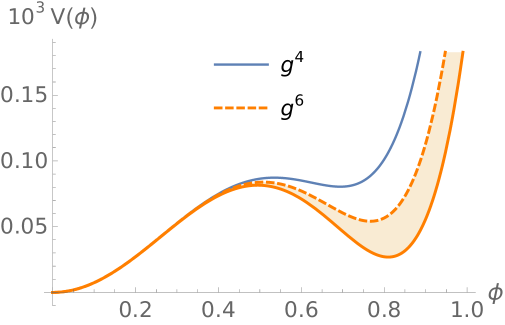
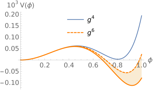
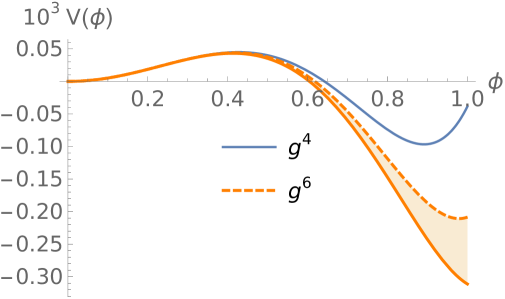
In Fig. 1, we depict this quantity at temperatures around the critical temperature , defined as that at which the scalar potential presents two degenerated minima. In Fig. 2, we show the nucleation temperature, the strength and the inverse duration time of the PT computed with the help of FindBounce [104], all derivative interactions being neglected 333A proper computation of the PT parameters should include the non-negligible effect of derivative interactions in the EFT, via appropriate perturbative functional analysis as worked out in Ref. [51]; see also Refs. [105, 106, 107]. It should also include higher-loop corrections [89, 108, 109, 110], to quartic and mass terms, as well as quantum corrections in the EFT [111, 112, 113, 114, 115, 116, 117] (e.g. the effective potential). This is beyond of the scope of our work though, and our naive estimation suffices to demonstrate the importance of terms in the SMEFT PT.. For each value of , we fix and to fit the Higgs vaccum expectation value GeV and the mass GeV at zero temperature.
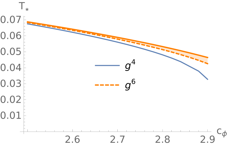
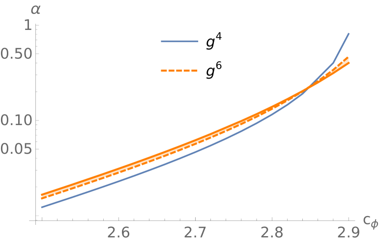
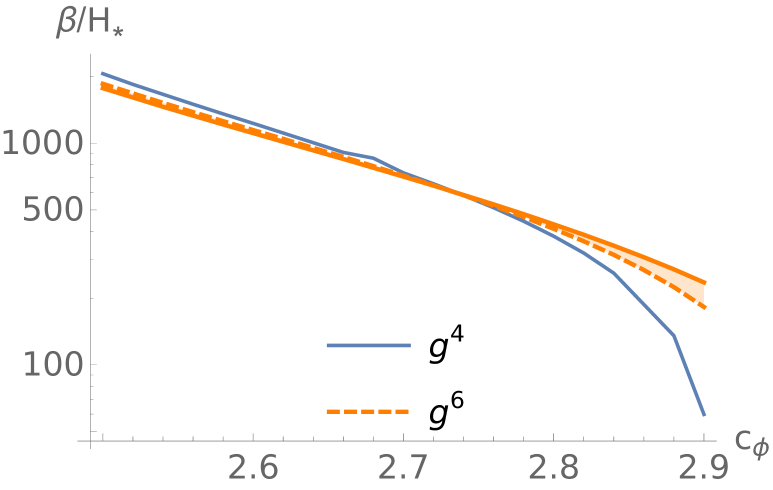
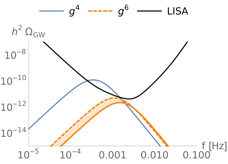
We also show the GW spectrum for , obtained with PTPlot [118, 61] (for simplicity we have simply assumed the bubble wall velocity to be . The sensitivity curve of LISA is drawn too. It is evident from the figure that corrections can modify the leading-order results by 50 % in the strongest PTs. This reflects in sizable changes in the GW spectrum. We have also checked that non-vanishing values for or reduce the allowed range of values for where a PT takes place. (We acknowledge that the large values of require a rather low cut-off. While the phenomenological viability of this has been discussed elsewhere [79, 84, 85, 76], here we simply use it as a toy example.)
Our work paves the way for accurate computations of thermal parameters (and most precisely of PT and GW ones) in the SMEFT, and so within any extension of the SM in which there is a gap between the new physics and the EW scales, and provided that . Still, achieving full requires a substantial amount of further computations. This includes, among others: (i) the extension of the 3-dimensional basis with gluonic operators [65, 28] (they do not intervene in the leading soft-scale Higgs potential, but they contribute at one loop); (ii) the computation of relevant 2- and 3-loop matching corrections, which would then involve 4-fermion SMEFT (see Ref. [89] for results within the SM); (iii) 2- and 3-loop running within the 3-dimensional theory; (iv) the EFT at the ultrasoft scale, resulting from integrating out the temporal components of 3-dimensional gauge fields with Debye masses; (v) the computation of the 3-loop effective potential. We plan to address some of these points in future works.
Acknowledgments
We are enormously grateful to Andreas Ekstedt for collaboration during the first stages of this project and for very detailed feedback on the manuscript. We thank L. Gil, J. López-Miras, P. Olgoso and J. Santiago for useful discussions. We are particularly thankful to Z. Ren for helping us with the generation of certain Green’s functions using an unpublished version of ABC4EFT [96]. MC acknowledges support from the MCIN/AEI (10.13039/501100011033) and ERDF (grants PID2021-128396NB-I00 and PID2022-139466NB-C22), from the Junta de Andalucía grants FQM 101 and P21-00199 and from Consejería de Universidad, Investigación e Innovación, Gobierno de España and Unión Europea – NextGenerationEU under grants AST22 6.5 and CNS2022-136024, as well as from the RyC program under contract number RYC2019-027155-I. The work of GG is supported by the Deutsche Forschungsgemeinschaft under Germany’s Excellence Strategy EXC 2121 “Quantum Universe” – 390833306, as well as by the grant 491245950.
References
- [1] P. H. Ginsparg, First Order and Second Order Phase Transitions in Gauge Theories at Finite Temperature, Nucl. Phys. B 170 (1980) 388–408.
- [2] T. Appelquist and R. D. Pisarski, High-Temperature Yang-Mills Theories and Three-Dimensional Quantum Chromodynamics, Phys. Rev. D 23 (1981) 2305.
- [3] T. Matsubara, A New approach to quantum statistical mechanics, Prog. Theor. Phys. 14 (1955) 351–378.
- [4] E. Braaten and A. Nieto, Effective field theory approach to high temperature thermodynamics, Phys. Rev. D 51 (1995) 6990–7006, [hep-ph/9501375].
- [5] K. Kajantie, M. Laine, K. Rummukainen and M. E. Shaposhnikov, Generic rules for high temperature dimensional reduction and their application to the standard model, Nucl. Phys. B 458 (1996) 90–136, [hep-ph/9508379].
- [6] A. Strumia and N. Tetradis, A Consistent calculation of bubble nucleation rates, Nucl. Phys. B 542 (1999) 719–741, [hep-ph/9806453].
- [7] J. Berges, N. Tetradis and C. Wetterich, Coarse graining and first order phase transitions, Phys. Lett. B 393 (1997) 387–394, [hep-ph/9610354].
- [8] D. Croon, O. Gould, P. Schicho, T. V. I. Tenkanen and G. White, Theoretical uncertainties for cosmological first-order phase transitions, JHEP 04 (2021) 055, [2009.10080].
- [9] O. Gould and T. V. I. Tenkanen, On the perturbative expansion at high temperature and implications for cosmological phase transitions, JHEP 06 (2021) 069, [2104.04399].
- [10] O. Gould and T. V. I. Tenkanen, Perturbative effective field theory expansions for cosmological phase transitions, JHEP 01 (2024) 048, [2309.01672].
- [11] K. Farakos, K. Kajantie, K. Rummukainen and M. E. Shaposhnikov, 3-D physics and the electroweak phase transition: Perturbation theory, Nucl. Phys. B 425 (1994) 67–109, [hep-ph/9404201].
- [12] K. Farakos, K. Kajantie, K. Rummukainen and M. E. Shaposhnikov, 3-d physics and the electroweak phase transition: A Framework for lattice Monte Carlo analysis, Nucl. Phys. B 442 (1995) 317–363, [hep-lat/9412091].
- [13] K. Kajantie, M. Laine, K. Rummukainen and M. E. Shaposhnikov, The Electroweak phase transition: A Nonperturbative analysis, Nucl. Phys. B 466 (1996) 189–258, [hep-lat/9510020].
- [14] M. Laine, Exact relation of lattice and continuum parameters in three-dimensional SU(2) + Higgs theories, Nucl. Phys. B 451 (1995) 484–504, [hep-lat/9504001].
- [15] M. Laine and A. Rajantie, Lattice continuum relations for 3-D SU(N) + Higgs theories, Nucl. Phys. B 513 (1998) 471–489, [hep-lat/9705003].
- [16] M. Gurtler, E.-M. Ilgenfritz and A. Schiller, Where the electroweak phase transition ends, Phys. Rev. D 56 (1997) 3888–3895, [hep-lat/9704013].
- [17] K. Rummukainen, M. Tsypin, K. Kajantie, M. Laine and M. E. Shaposhnikov, The Universality class of the electroweak theory, Nucl. Phys. B 532 (1998) 283–314, [hep-lat/9805013].
- [18] M. Laine and K. Rummukainen, What’s new with the electroweak phase transition?, Nucl. Phys. B Proc. Suppl. 73 (1999) 180–185, [hep-lat/9809045].
- [19] G. D. Moore and K. Rummukainen, Electroweak bubble nucleation, nonperturbatively, Phys. Rev. D 63 (2001) 045002, [hep-ph/0009132].
- [20] P. B. Arnold and G. D. Moore, Monte Carlo simulation of O(2) phi**4 field theory in three-dimensions, Phys. Rev. E 64 (2001) 066113, [cond-mat/0103227].
- [21] X.-p. Sun, Monte Carlo studies of three-dimensional O(1) and O(4) phi**4 theory related to BEC phase transition temperatures, Phys. Rev. E 67 (2003) 066702, [hep-lat/0209144].
- [22] M. D’Onofrio and K. Rummukainen, Standard model cross-over on the lattice, Phys. Rev. D 93 (2016) 025003, [1508.07161].
- [23] O. Gould, S. Güyer and K. Rummukainen, First-order electroweak phase transitions: A nonperturbative update, Phys. Rev. D 106 (2022) 114507, [2205.07238].
- [24] E. Braaten, Solution to the perturbative infrared catastrophe of hot gauge theories, Phys. Rev. Lett. 74 (1995) 2164–2167, [hep-ph/9409434].
- [25] E. Braaten and A. Nieto, Free energy of QCD at high temperature, Phys. Rev. D 53 (1996) 3421–3437, [hep-ph/9510408].
- [26] K. Kajantie, M. Laine, K. Rummukainen and M. E. Shaposhnikov, 3-D SU(N) + adjoint Higgs theory and finite temperature QCD, Nucl. Phys. B 503 (1997) 357–384, [hep-ph/9704416].
- [27] M. Laine, P. Schicho and Y. Schröder, A QCD Debye mass in a broad temperature range, Phys. Rev. D 101 (2020) 023532, [1911.09123].
- [28] M. Laine, P. Schicho and Y. Schröder, Soft thermal contributions to 3-loop gauge coupling, JHEP 05 (2018) 037, [1803.08689].
- [29] J. Ghiglieri, G. D. Moore, P. Schicho and N. Schlusser, The force-force-correlator in hot QCD perturbatively and from the lattice, JHEP 02 (2022) 058, [2112.01407].
- [30] T. Brauner, T. V. I. Tenkanen, A. Tranberg, A. Vuorinen and D. J. Weir, Dimensional reduction of the Standard Model coupled to a new singlet scalar field, JHEP 03 (2017) 007, [1609.06230].
- [31] J. O. Andersen, T. Gorda, A. Helset, L. Niemi, T. V. I. Tenkanen, A. Tranberg et al., Nonperturbative Analysis of the Electroweak Phase Transition in the Two Higgs Doublet Model, Phys. Rev. Lett. 121 (2018) 191802, [1711.09849].
- [32] L. Niemi, H. H. Patel, M. J. Ramsey-Musolf, T. V. I. Tenkanen and D. J. Weir, Electroweak phase transition in the real triplet extension of the SM: Dimensional reduction, Phys. Rev. D 100 (2019) 035002, [1802.10500].
- [33] T. Gorda, A. Helset, L. Niemi, T. V. I. Tenkanen and D. J. Weir, Three-dimensional effective theories for the two Higgs doublet model at high temperature, JHEP 02 (2019) 081, [1802.05056].
- [34] K. Kainulainen, V. Keus, L. Niemi, K. Rummukainen, T. V. I. Tenkanen and V. Vaskonen, On the validity of perturbative studies of the electroweak phase transition in the Two Higgs Doublet model, JHEP 06 (2019) 075, [1904.01329].
- [35] O. Gould, J. Kozaczuk, L. Niemi, M. J. Ramsey-Musolf, T. V. I. Tenkanen and D. J. Weir, Nonperturbative analysis of the gravitational waves from a first-order electroweak phase transition, Phys. Rev. D 100 (2019) 115024, [1903.11604].
- [36] L. Niemi, M. J. Ramsey-Musolf, T. V. I. Tenkanen and D. J. Weir, Thermodynamics of a Two-Step Electroweak Phase Transition, Phys. Rev. Lett. 126 (2021) 171802, [2005.11332].
- [37] O. Gould and J. Hirvonen, Effective field theory approach to thermal bubble nucleation, Phys. Rev. D 104 (2021) 096015, [2108.04377].
- [38] O. Gould, Real scalar phase transitions: a nonperturbative analysis, JHEP 04 (2021) 057, [2101.05528].
- [39] P. M. Schicho, T. V. I. Tenkanen and J. Österman, Robust approach to thermal resummation: Standard Model meets a singlet, JHEP 06 (2021) 130, [2102.11145].
- [40] J. Löfgren, M. J. Ramsey-Musolf, P. Schicho and T. V. I. Tenkanen, Nucleation at Finite Temperature: A Gauge-Invariant Perturbative Framework, Phys. Rev. Lett. 130 (2023) 251801, [2112.05472].
- [41] L. Niemi, P. Schicho and T. V. I. Tenkanen, Singlet-assisted electroweak phase transition at two loops, Phys. Rev. D 103 (2021) 115035, [2103.07467].
- [42] L. Niemi, K. Rummukainen, R. Seppä and D. J. Weir, Infrared physics of the 3D SU(2) adjoint Higgs model at the crossover transition, JHEP 02 (2023) 212, [2206.14487].
- [43] A. Ekstedt, Convergence of the nucleation rate for first-order phase transitions, Phys. Rev. D 106 (2022) 095026, [2205.05145].
- [44] A. Ekstedt, O. Gould and J. Löfgren, Radiative first-order phase transitions to next-to-next-to-leading order, Phys. Rev. D 106 (2022) 036012, [2205.07241].
- [45] S. Biondini, P. Schicho and T. V. I. Tenkanen, Strong electroweak phase transition in t-channel simplified dark matter models, JCAP 10 (2022) 044, [2207.12207].
- [46] P. Schicho, T. V. I. Tenkanen and G. White, Combining thermal resummation and gauge invariance for electroweak phase transition, JHEP 11 (2022) 047, [2203.04284].
- [47] O. Gould and C. Xie, Higher orders for cosmological phase transitions: a global study in a Yukawa model, JHEP 12 (2023) 049, [2310.02308].
- [48] M. Kierkla, B. Swiezewska, T. V. I. Tenkanen and J. van de Vis, Gravitational waves from supercooled phase transitions: dimensional transmutation meets dimensional reduction, JHEP 02 (2024) 234, [2312.12413].
- [49] G. Aarts et al., Phase Transitions in Particle Physics: Results and Perspectives from Lattice Quantum Chromo-Dynamics, Prog. Part. Nucl. Phys. 133 (2023) 104070, [2301.04382].
- [50] L. Niemi, M. J. Ramsey-Musolf and G. Xia, Nonperturbative study of the electroweak phase transition in the real scalar singlet extended standard model, Phys. Rev. D 110 (2024) 115016, [2405.01191].
- [51] M. Chala, J. C. Criado, L. Gil and J. L. Miras, Higher-order-operator corrections to phase-transition parameters in dimensional reduction, JHEP 10 (2024) 025, [2406.02667].
- [52] R. Qin and L. Bian, First-order electroweak phase transition at finite density, JHEP 08 (2024) 157, [2407.01981].
- [53] O. Gould and P. Saffin, Perturbative gravitational wave predictions for the real-scalar extended Standard Model, 2411.08951.
- [54] L. Niemi and T. V. I. Tenkanen, Investigating two-loop effects for first-order electroweak phase transitions, 2408.15912.
- [55] M. Kierkla, P. Schicho, B. Swiezewska, T. V. I. Tenkanen and J. van de Vis, Finite-temperature bubble nucleation with shifting scale hierarchies, 2503.13597.
- [56] LIGO Scientific collaboration, J. Aasi et al., Advanced LIGO, Class. Quant. Grav. 32 (2015) 074001, [1411.4547].
- [57] NANOGrav collaboration, Z. Arzoumanian et al., The NANOGrav 12.5 yr Data Set: Search for an Isotropic Stochastic Gravitational-wave Background, Astrophys. J. Lett. 905 (2020) L34, [2009.04496].
- [58] G. M. Harry, P. Fritschel, D. A. Shaddock, W. Folkner and E. S. Phinney, Laser interferometry for the big bang observer, Class. Quant. Grav. 23 (2006) 4887–4894.
- [59] S. Kawamura et al., The Japanese space gravitational wave antenna DECIGO, Class. Quant. Grav. 23 (2006) S125–S132.
- [60] W.-H. Ruan, Z.-K. Guo, R.-G. Cai and Y.-Z. Zhang, Taiji program: Gravitational-wave sources, Int. J. Mod. Phys. A 35 (2020) 2050075, [1807.09495].
- [61] C. Caprini et al., Detecting gravitational waves from cosmological phase transitions with LISA: an update, JCAP 03 (2020) 024, [1910.13125].
- [62] J. E. Camargo-Molina, R. Enberg and J. Löfgren, A new perspective on the electroweak phase transition in the Standard Model Effective Field Theory, JHEP 10 (2021) 127, [2103.14022].
- [63] E. Camargo-Molina, R. Enberg and J. Löfgren, A Catalog of First-Order Electroweak Phase Transitions in the Standard Model Effective Field Theory, 2410.23210.
- [64] A. Ekstedt, P. Schicho and T. V. I. Tenkanen, DRalgo: A package for effective field theory approach for thermal phase transitions, Comput. Phys. Commun. 288 (2023) 108725, [2205.08815].
- [65] S. Chapman, A New dimensionally reduced effective action for QCD at high temperature, Phys. Rev. D 50 (1994) 5308–5313, [hep-ph/9407313].
- [66] G. D. Moore, Fermion determinant and the sphaleron bound, Phys. Rev. D 53 (1996) 5906–5917, [hep-ph/9508405].
- [67] J. Chakrabortty and S. Mohanty, One Loop Thermal Effective Action, 2411.14146.
- [68] F. Bernardo, P. Klose, P. Schicho and T. V. I. Tenkanen, Higher-dimensional operators at finite-temperature affect gravitational-wave predictions, 2025.
- [69] K. Kajantie, M. Laine, K. Rummukainen and M. E. Shaposhnikov, High temperature dimensional reduction and parity violation, Phys. Lett. B 423 (1998) 137–144, [hep-ph/9710538].
- [70] X.-m. Zhang, Operators analysis for Higgs potential and cosmological bound on Higgs mass, Phys. Rev. D 47 (1993) 3065–3067, [hep-ph/9301277].
- [71] D. Bodeker, L. Fromme, S. J. Huber and M. Seniuch, The Baryon asymmetry in the standard model with a low cut-off, JHEP 02 (2005) 026, [hep-ph/0412366].
- [72] C. Grojean, G. Servant and J. D. Wells, First-order electroweak phase transition in the standard model with a low cutoff, Phys. Rev. D 71 (2005) 036001, [hep-ph/0407019].
- [73] S. W. Ham and S. K. Oh, Electroweak phase transition in the standard model with a dimension-six Higgs operator at one-loop level, Phys. Rev. D 70 (2004) 093007, [hep-ph/0408324].
- [74] C. Delaunay, C. Grojean and J. D. Wells, Dynamics of Non-renormalizable Electroweak Symmetry Breaking, JHEP 04 (2008) 029, [0711.2511].
- [75] B. Grinstein and M. Trott, Electroweak Baryogenesis with a Pseudo-Goldstone Higgs, Phys. Rev. D 78 (2008) 075022, [0806.1971].
- [76] P. H. Damgaard, A. Haarr, D. O’Connell and A. Tranberg, Effective Field Theory and Electroweak Baryogenesis in the Singlet-Extended Standard Model, JHEP 02 (2016) 107, [1512.01963].
- [77] J. de Vries, M. Postma, J. van de Vis and G. White, Electroweak Baryogenesis and the Standard Model Effective Field Theory, JHEP 01 (2018) 089, [1710.04061].
- [78] R.-G. Cai, M. Sasaki and S.-J. Wang, The gravitational waves from the first-order phase transition with a dimension-six operator, JCAP 08 (2017) 004, [1707.03001].
- [79] M. Chala, C. Krause and G. Nardini, Signals of the electroweak phase transition at colliders and gravitational wave observatories, JHEP 07 (2018) 062, [1802.02168].
- [80] J. Ellis, M. Lewicki and J. M. No, On the Maximal Strength of a First-Order Electroweak Phase Transition and its Gravitational Wave Signal, JCAP 04 (2019) 003, [1809.08242].
- [81] J. Ellis, M. Lewicki, J. M. No and V. Vaskonen, Gravitational wave energy budget in strongly supercooled phase transitions, JCAP 06 (2019) 024, [1903.09642].
- [82] J. Ellis, M. Fairbairn, M. Lewicki, V. Vaskonen and A. Wickens, Intergalactic Magnetic Fields from First-Order Phase Transitions, JCAP 09 (2019) 019, [1907.04315].
- [83] V. Q. Phong, P. H. Khiem, N. P. D. Loc and H. N. Long, Sphaleron in the first-order electroweak phase transition with the dimension-six Higgs field operator, Phys. Rev. D 101 (2020) 116010, [2003.09625].
- [84] M. Postma and G. White, Cosmological phase transitions: is effective field theory just a toy?, JHEP 03 (2021) 280, [2012.03953].
- [85] K. Hashino and D. Ueda, SMEFT effects on the gravitational wave spectrum from an electroweak phase transition, Phys. Rev. D 107 (2023) 095022, [2210.11241].
- [86] S. Kanemura, R. Nagai and M. Tanaka, Electroweak phase transition in the nearly aligned Higgs effective field theory, JHEP 06 (2022) 027, [2202.12774].
- [87] R. Alonso, J. C. Criado, R. Houtz and M. West, Walls, bubbles and doom — the cosmology of HEFT, JHEP 05 (2024) 049, [2312.00881].
- [88] V. K. Oikonomou and A. Giovanakis, Electroweak phase transition in singlet extensions of the standard model with dimension-six operators, Phys. Rev. D 109 (2024) 055044, [2403.01591].
- [89] A. Gynther and M. Vepsalainen, Pressure of the standard model at high temperatures, JHEP 01 (2006) 060, [hep-ph/0510375].
- [90] W. Buchmuller and D. Wyler, Effective Lagrangian Analysis of New Interactions and Flavor Conservation, Nucl. Phys. B 268 (1986) 621–653.
- [91] B. Grzadkowski, M. Iskrzynski, M. Misiak and J. Rosiek, Dimension-Six Terms in the Standard Model Lagrangian, JHEP 10 (2010) 085, [1008.4884].
- [92] I. Brivio and M. Trott, The Standard Model as an Effective Field Theory, Phys. Rept. 793 (2019) 1–98, [1706.08945].
- [93] G. Isidori, F. Wilsch and D. Wyler, The standard model effective field theory at work, Rev. Mod. Phys. 96 (2024) 015006, [2303.16922].
- [94] J. C. Criado, BasisGen: automatic generation of operator bases, Eur. Phys. J. C 79 (2019) 256, [1901.03501].
- [95] R. M. Fonseca, The Sym2Int program: going from symmetries to interactions, J. Phys. Conf. Ser. 873 (2017) 012045, [1703.05221].
- [96] H.-L. Li, Z. Ren, M.-L. Xiao, J.-H. Yu and Y.-H. Zheng, Operators for generic effective field theory at any dimension: on-shell amplitude basis construction, JHEP 04 (2022) 140, [2201.04639].
- [97] L. F. Abbott, Introduction to the Background Field Method, Acta Phys. Polon. B 13 (1982) 33.
- [98] A. Alloul, N. D. Christensen, C. Degrande, C. Duhr and B. Fuks, FeynRules 2.0 - A complete toolbox for tree-level phenomenology, Comput. Phys. Commun. 185 (2014) 2250–2300, [1310.1921].
- [99] T. Hahn, Generating Feynman diagrams and amplitudes with FeynArts 3, Comput. Phys. Commun. 140 (2001) 418–431, [hep-ph/0012260].
- [100] V. Shtabovenko, R. Mertig and F. Orellana, New Developments in FeynCalc 9.0, Comput. Phys. Commun. 207 (2016) 432–444, [1601.01167].
- [101] Q. Bonnefoy, E. Gendy, C. Grojean and J. T. Ruderman, Beyond Jarlskog: 699 invariants for CP violation in SMEFT, JHEP 08 (2022) 032, [2112.03889].
- [102] M. Chala, G. Guedes, M. Ramos and J. Santiago, Towards the renormalisation of the Standard Model effective field theory to dimension eight: Bosonic interactions I, SciPost Phys. 11 (2021) 065, [2106.05291].
- [103] M. Chala, A. Díaz-Carmona and G. Guedes, A Green’s basis for the bosonic SMEFT to dimension 8, JHEP 05 (2022) 138, [2112.12724].
- [104] V. Guada, M. Nemevšek and M. Pintar, FindBounce: Package for multi-field bounce actions, Comput. Phys. Commun. 256 (2020) 107480, [2002.00881].
- [105] J. Baacke and A. Surig, Computing numerically the functional derivative of an effective action, Z. Phys. C 73 (1997) 369–378, [hep-ph/9511231].
- [106] J. Hirvonen, J. Löfgren, M. J. Ramsey-Musolf, P. Schicho and T. V. I. Tenkanen, Computing the gauge-invariant bubble nucleation rate in finite temperature effective field theory, JHEP 07 (2022) 135, [2112.08912].
- [107] B. Hua and J. Zhu, VacuumTunneling: A package to solve bounce equation with renormalization factor, 2501.15236.
- [108] I. Ghisoiu and Y. Schroder, A new three-loop sum-integral of mass dimension two, JHEP 09 (2012) 016, [1207.6214].
- [109] Y. Schroder, A fresh look on three-loop sum-integrals, JHEP 08 (2012) 095, [1207.5666].
- [110] A. I. Davydychev, P. Navarrete and Y. Schröder, Factorizing two-loop vacuum sum-integrals, JHEP 02 (2024) 104, [2312.17367].
- [111] J. Baacke and V. G. Kiselev, One loop corrections to the bubble nucleation rate at finite temperature, Phys. Rev. D 48 (1993) 5648–5654, [hep-ph/9308273].
- [112] G. V. Dunne and H. Min, Beyond the thin-wall approximation: Precise numerical computation of prefactors in false vacuum decay, Phys. Rev. D 72 (2005) 125004, [hep-th/0511156].
- [113] W.-Y. Ai, B. Garbrecht and P. Millington, Radiative effects on false vacuum decay in Higgs-Yukawa theory, Phys. Rev. D 98 (2018) 076014, [1807.03338].
- [114] W.-Y. Ai, J. S. Cruz, B. Garbrecht and C. Tamarit, Gradient effects on false vacuum decay in gauge theory, Phys. Rev. D 102 (2020) 085001, [2006.04886].
- [115] A. Ekstedt, O. Gould and J. Hirvonen, BubbleDet: a Python package to compute functional determinants for bubble nucleation, JHEP 12 (2023) 056, [2308.15652].
- [116] W.-Y. Ai, J. Alexandre and S. Sarkar, False vacuum decay rates, more precisely, Phys. Rev. D 109 (2024) 045010, [2312.04482].
- [117] M. Matteini, M. Nemevšek, Y. Shoji and L. Ubaldi, False Vacuum Decay Rate From Thin To Thick Walls, 2404.17632.
- [118] D. J. Weir, PTPlot: a tool for exploring the gravitational wave power spectrum from first-order phase transitions, Zenodo (2022) .