A Cartesian catalog of 30 million Gaia sources based on second-order and Monte Carlo error propagation

Abstract

Accurate measurements of stellar positions and velocities are crucial for studying galactic and stellar dynamics. We aim to create a Cartesian catalog from Gaia DR3 to serve as a high-precision database for further research using stellar coordinates and velocities. To avoid the negative parallax values, we select 31,129,169 sources in Gaia DR3 with radial velocity, where the fractional parallax error is less than 20% ($0<\sigma_{\varpi}/\varpi<0.2$). To select the most accurate and efficient method of propagating mean and covariance, we use the Monte Carlo results with $10^{7}$ samples (MC7) as the benchmark, and compare the precision of linear, second-order, and Monte Carlo error propagation methods. By assessing the accuracy of propagated mean and covariance, we observe that second-order error propagation exhibits mean deviations of at most 0.5% compared to MC7, with variance deviations of up to 10%. Overall, this outperforms linear transformation. Though Monte Carlo method with $10^{4}$ samples (MC4) is an order of magnitude slower than second-order error propagation, its covariances propagation accuracy reaches 1% when $\sigma_{\varpi}/\varpi$ is below 15%. Consequently, we employ second-order error propagation to convert the mean astrometry and radial velocity into Cartesian coordinates and velocities in both equatorial and galactic systems for 30 million Gaia sources, and apply MC4 for covariance propagation. The Cartesian catalog and source code are provided for future applications in high-precision stellar and galactic dynamics.

1 Introduction

The demand for high-precision reconstruction of stellar orbits has gained prominence, particularly with the emergence of advanced astrometric missions like Gaia (Gaia Collaboration et al. 2016b, 2018). Gaia Data Release 3 (DR3) offers the largest collection of all-sky spectrophotometry, radial velocities, and astrophysical parameters for stars. It is highly accurate in astrometric measurements for $\rm{G<15~mag}$, with median position uncertainties ranging from 0.01 to 0.02 mas, median parallax uncertainties between 0.02 and 0.03 mas, median proper motion uncertainties from 0.02 to 0.03 mas/yr, and the radial velocity uncertainty of approximately 1 km/s (Gaia Collaboration et al. 2021, 2023). Such extraordinary precision in data has become a cornerstone in Galactic and stellar dynamics research, unlocking new possibilities for understanding the intricacies of celestial motion and providing unprecedented insights into the structures and dynamics of our galaxy.

We can resolve individual stars in and around our host Galaxy, the Milky Way (MW). These include the stars in tidal debris or stellar streams, which are stripped by tidal forces from dwarf galaxies and globular clusters orbiting around the MW. In the field of galactic dynamics, the modeling of stellar streams often combines an approximate treatment of the stream formation to a high resolution simulation of galaxy formation. For streams whose progenitor galaxy or globular cluster are not fully disrupted by tides, the currently observed position and velocity of the progenitor can be integrated back in time with a fiducial MW potential model. It is then integrated forward in time, with tracer particles released from the two Lagrangian points to simulate the formation and evolution of the stream in the galactic tidal field. By comparing the simulated stream to the observation, one can constrain the underlying dark matter distribution (e.g. Küpper et al. 2012; Bonaca et al. 2014; Küpper et al. 2015; Gibbons et al. 2017; Palau & Miralda-Escudé 2023). The modeling of stream orbit strongly depends on the initial condition set up by the Cartesian coordinates of the progenitors, and is often achieved in action and action-frequency space (e.g. Sanders & Binney 2013; Bovy 2014; Sanders 2014; Bovy et al. 2016), hence sensitive to error propagation.

In the pursuit of understanding wide binaries, achieving precise error propagation is paramount, given the subtle velocity differences, often as minimal as $\sim$1 kms^-1, exhibited by these binary systems. Harnessing the high-precision astrometric data generously provided by Gaia (Gaia Collaboration et al. 2016a), millions of wide binaries are identified through the meticulous examination of their common proper motion and parallax (e.g., El-Badry & Rix 2018; Tian et al. 2020; El-Badry et al. 2021). Particularly noteworthy is the utilization of the relative velocity and relative position angle of wide binaries to explore their eccentricity distribution (Hwang et al. 2022). Given that these investigations heavily rely on the accurate Cartesian coordinates and velocities of stars, the precise transformation of coordinates from Gaia astrometry, coupled with meticulous error propagation, becomes imperative. This is not only crucial for avoiding false positives in wide binary selection but also for enhancing the reliability of statistical studies concerning their properties.

Unlike wide binaries, stellar encounters encompass the serendipitous alignment of stars, occurring when they come into close proximity over a relatively short period. Notably, stellar encounters within the solar system significantly contribute to shaping the structure of the Oort Cloud (e.g., García-Sánchez et al. 2001; Dones et al. 2004; Rickman et al. 2008, 2012; Feng & Bailer-Jones 2015; Dybczyński et al. 2022) . The exploration of slow and close encounters, involving interstellar objects like ‘Oumuamua, yields valuable insights into identifying their home systems and understanding their dynamical history (e.g., Feng & Jones 2018b; Bailer-Jones et al. 2018; Zwart et al. 2018; Loeb 2022). Accurate stellar orbital integration proves essential in pinpointing stellar encounters, necessitating the precise propagation of stellar motion from an initial epoch to millions of years in the past or future. Given the nonlinear nature of stellar orbits over a million-year time scale, the encounter time and distance are highly sensitive to the initial Cartesian state of the stars (Dybczyński & Berski 2015).

Recognizing the critical role of error propagation in numerous astrophysical applications, we undertake a comparative analysis of different methodologies for error propagation in the transformation of Gaia astrometry into Cartesian positions and velocities of stars. Specifically, we investigate the linear, second-order, and Monte Carlo (MC) error propagation methods. While advanced techniques such as the Kalman filter and unscented transformation (e.g., Smith et al. 1962; Schmidt 1966; Julier & Uhlmann 2004; Chen et al. 2017; Michelotti et al. 2024) are commonly applied in nonlinear-system tracking and navigation, second-order error propagation consistently achieves precision comparable to these approaches. This is exemplified by Feng & Jones (2018a), who conducted a comprehensive comparison of various methods in the orbital integration of stars. Our study reaffirms that second-order error propagation surpasses linear propagation in accuracy. Consequently, we use second-order error propagation to derive Cartesian positions and velocities in both Equatorial and Galactic coordinate systems from Gaia astrometry, and apply MC with $10^{4}$ samples for covariance conversion. This approach not only enhances the efficiency and accuracy of coordinate transformation but also establishes a robust foundation for research across diverse astrophysical fields.

The structure of this paper unfolds as follows: In section 2, we provide a detailed overview of the research analysis, elucidating the data employed for error propagation. Section 3 delves into the techniques utilized for coordinate transformation and covariance propagation, encompassing MC, linear, and second-order error propagation methods. Transitioning to section 4, we present and discuss the extensive outcomes derived from our methodology, focusing on approximately 30 million sources in the Gaia DR3. Lastly, section 5 encapsulates a succinct discussion and conclusion.

2 Data

Gaia Data Release 3 (DR3; Gaia Collaboration et al. 2023) encompasses 33,812,183 sources, providing the measurements of radial velocities ($v_{r}$) and five-parameter astrometric data, including Right Ascension (R.A.; $\alpha$), Declination (decl.; $\delta$), parallaxes ($\varpi$), proper motions in R.A. ($\mu_{\alpha}$) and proper motions in decl. ($\mu_{\delta}$). Due to more observational data and improved data reduction pipeline, Gaia DR3 provides much more targets with radial velocity data than the 7,224,631 sources provided by Gaia Data Release 2 (DR2; Gaia Collaboration et al. 2018), and the accuracy of radial velocity has also been significantly improved Katz, D. et al. (2023).

While distance is inherently a positive quantity, in some instances, sources may exhibit negative parallaxes due to various reasons. Bayesian inference has been adopted to estimate the distances for stars with negative parallax measurements (e.g., Astraatmadja & Bailer-Jones 2016; Luri, X. et al. 2018; Bailer-Jones et al. 2018, 2021). Following the recommendation of Bailer-Jones (2015), incorporating appropriate priors becomes crucial for Gaia sources with fractional parallax error ($\sigma_{\varpi}/\varpi$) exceeding 20% for distance inference. However, targets with precise parallax measurements ($0<\sigma_{\varpi}/\varpi<0.2$) and high signal to noise ($S/N>5$) are not sensitive to priors (e.g., Bromley et al. 2018).

Consequently, after correcting for zero-point offset in parallax (Lindegren et al. 2021; Ding et al. 2024), as well as magnitude and color-dependent proper motion bias (Cantat-Gaudin, Tristan & Brandt, Timothy D. 2021), we select a subset of 31,129,169 stars from Gaia DR3, which have valid radial velocity measurements and have fractional parallax error satisfying $0<\sigma_{\varpi}/\varpi<0.2~.$ This allows distance to be directly represented by the reciprocal of parallax, ensuring reliability and accuracy while minimizing potential bias from priors.

3 Error propagation

In this section, we delineate three error propagation methods utilized in this study. Our approach involves converting the five-parameter astrometry and radial velocities of Gaia sources to Cartesian coordinates and velocities in both the Equatorial and Galactic coordinate systems. Additional details regarding the transformation of galactic coordinates can be found in Appendix B.

3.1 Linear error propagation

Linear error propagation is the default method used by the most astronomical data analyses. Considering that linear error propagation is broadly used in the community (e.g. Butkevich & Lindegren 2014), we only briefly introduce the linear error propagation as follows.

First of all, we define the vectors and matrices that will be used in error propagation. The spherical ($\rm sph$) position and velocity vector in the equatorial coordinate system is defined as:

$${\bm{\xi}}_{\rm sph}\equiv\begin{bmatrix}\alpha\\ \delta\\ \varpi\\ \mu_{\alpha^{*}}\\ \mu_{\delta}\\ v_{r}\end{bmatrix}~.$$ (1)

The distance $r$ is derived from the parallax according to $r=\frac{\rm A}{\varpi}~$, where $\rm{A}=1\,\rm{AU}$. The position and velocity vector in Cartesian equatorial ($\rm eqt$) coordinates is linked to the spherical coordinates as:

$${\bm{\xi}}_{\rm eqt}\equiv\begin{bmatrix}x\\ y\\ z\\ v_{x}\\ v_{y}\\ v_{z}\end{bmatrix}=\begin{bmatrix}r\cos{\delta}\cos{\alpha}\\ r\cos{\delta}\sin{\alpha}\\ r\sin{\delta}\\ v_{r}\cos{\delta}\cos{\alpha}-r\mu_{\alpha^{*}}\sin{\alpha}-r\mu_{\delta}\sin{\delta}\cos{\alpha}\\ v_{r}\cos{\delta}\sin{\alpha}+r\mu_{\alpha^{*}}\cos{\alpha}-r\mu_{\delta}\sin{\delta}\sin{\alpha}\\ r\mu_{\delta}\cos{\delta}+v_{r}\sin{\delta}\end{bmatrix}~.$$ (2)

The Gaia DR3 catalog provides the uncertainties, the corresponding correlation coefficients of the five-parameter astrometric solutions, and the errors of radial velocities. Considering that the radial velocity and the five-parameter astrometry are measured independently, we treat the five astrometric parameters as independent of the radial velocity. Hence the correlation coefficients between $v_{r}$ and the five astrometric parameters are zero. From Gaia DR3, we change $\sigma_{\alpha^{*}}$ to $\sigma_{\alpha}$, and use $\vec{\sigma}=(\sigma_{\alpha},\sigma_{\delta},\sigma_{\varpi},\sigma_{\mu_{\alpha^{*}}},\sigma_{\mu_{\delta}},\sigma_{v_{r}})$ to denote the errors in the position and velocity vectors for sources, and $\rho_{ij}\,(=\rho_{ji})$ to denote the corresponding correlation coefficient, with i or j representing $\alpha$, $\delta$, $\varpi$, $\mu_{\alpha^{*}}$, $\mu_{\delta}$, or $v_{r}$. The six-dimensional variance-covariance matrix (or covariance matrix) is:

$$\bm{C}_{\rm sph}=\begin{bmatrix}\sigma^{2}_{\alpha}&\sigma_{\alpha}\sigma_{\delta}\rho_{\alpha\delta}&\cdots&\sigma_{\alpha}\sigma_{\mu_{\delta}}\rho_{\alpha\mu_{\delta}}&0\\ \sigma_{\delta}\sigma_{\alpha}\rho_{\alpha\delta}&\sigma_{\delta}^{2}&\cdots&\sigma_{\delta}\sigma_{\mu_{\delta}}\rho_{\delta\mu_{\delta}}&0\\ \vdots&\vdots&\ddots&\vdots&\vdots\\ \sigma_{\mu_{\delta}}\sigma_{\alpha}\rho_{\alpha\mu_{\delta}}&\sigma_{\mu_{\delta}}\sigma_{\delta}\rho_{\delta\mu_{\delta}}&\cdots&\sigma_{\mu_{\delta}}^{2}&0\\ 0&0&\cdots&0&\sigma_{v_{r}}^{2}\end{bmatrix}~.$$ (3)

The transformation from spherical coordinates to Cartesian coordinates requires the utilization of the Jacobian matrix:

$$\bm{J}=\frac{\partial{(x,y,z,v_{x},v_{y},v_{z})}}{\partial{(\alpha,\delta,\varpi,\mu_{\alpha^{*}},\mu_{\delta},v_{r})}}=\begin{bmatrix}\frac{\partial{x}}{\partial{\alpha}}&\frac{\partial{x}}{\partial{\delta}}&\cdots&\frac{\partial{x}}{\partial{v_{r}}}\\ \frac{\partial{y}}{\partial{\alpha}}&\frac{\partial{y}}{\partial{\delta}}&\cdots&\frac{\partial{y}}{\partial{v_{r}}}\\ \vdots&\vdots&\ddots&\vdots\\ \frac{\partial{v_{z}}}{\partial{\alpha}}&\frac{\partial{v_{z}}}{\partial{\delta}}&\cdots&\frac{\partial{v_{z}}}{\partial{v_{r}}}\end{bmatrix}~,$$ (4)

see Appendix C for details of the Jacobian matrix. Therefore, the conversion from a covariance matrix in spherical coordinates to one in Cartesian equatorial coordinates can be expressed as:

$$\bm{C}_{\rm eqt}=\bm{J}\bm{C}_{\rm sph}\bm{J}^{T}~.$$ (5)

3.2 Second-order error propagation

Although linear propagation is widely used, it may not always yield the best results for accurate error propagation (e.g. Ilyin 2012). Therefore, higher order error propagation is necessary to ensure optimal performance in certain cases. Specifically, when dealing with measurements that have relatively large errors, the truncation errors of the Taylor series can become significant. In such scenarios, the use of a linear transformation may result in decreased accuracy. To solve this problem and achieve enhanced precision, it is necessary to employ a second-order Taylor series for propagating statistical errors.

Second-order error propagation is commonly used in science and engineering, especially for precise calculations and data processing (Wang & Chirikjian 2008; Le Dimet et al. 2014). In astronomy, second-order error propagation is frequently applied to measure the position and motion of celestial bodies, such as satellite orbit calculations (e.g., Sengupta et al. 2007; Li & Sang 2020).

Following Putko et al. (2001), the second-order mean and variance of the output vector $\bm{F}$, transformed from those of the input vector $\bm{b}$, can be expressed as follows:

$$\bm{\bar{F}}=\bm{F(\bar{b})}+\frac{1}{2!}\sum_{j=1}^{n}\sum_{i=1}^{n}\frac{\partial^{2}{\bm{F}}}{\partial{b_{i}}\partial{b_{j}}}\sigma_{b_{i}}\sigma_{b_{j}}~,$$ (6)

$$\sigma_{F}^{2}=\sum_{i=1}^{n}(\frac{\partial{\bm{F}}}{\partial{b_{i}}}\sigma_{b_{i}})^{2}+\frac{1}{2!}\sum_{j=1}^{n}\sum_{i=1}^{n}(\frac{\partial^{2}{\bm{F}}}{\partial{b_{i}}\partial{b_{j}}}\sigma_{b_{i}}\sigma_{b_{j}})^{2}~,$$ (7)

where $\bm{F(\bar{b})}$ and $\sum_{i=1}^{n}(\frac{\partial{\bm{F}}}{\partial{b_{i}}}\sigma_{b_{i}})^{2}$ are the first-order mean and variance.

When the Hessian matrix $\bm{H}$ and the covariance matrix $\bm{C}$ are available, calculations of the second-order moments about vector $\bm{F}$ and variables $b_{i}$, where i=1,…,n, can be performed using matrix operations (see Zhang et al. (2011) for detailed definitions and derivation).

In matrix form, the second-order terms in the aforementioned equations can be expressed as:

$$\sum_{j=1}^{n}\sum_{i=1}^{n}\frac{\partial^{2}{\bm{F}}}{\partial{b_{i}}\partial{b_{j}}}\sigma_{b_{i}}\sigma_{b_{j}}=tr(\bm{HC})~,$$ (8)

$$\sum_{j=1}^{n}\sum_{i=1}^{n}(\frac{\partial^{2}{\bm{F}}}{\partial{b_{i}}\partial{b_{j}}}\sigma_{b_{i}}\sigma_{b_{j}})^{2}=tr(\bm{HCHC})~.$$ (9)

Performing a Taylor series expansion at a particular point provides results that hold true only in the immediate proximity of that point. Consequently, the precision of the approximation tends to diminish as the deviation from the mean grows, particularly when dealing with a non-Gaussian distribution of the output vector. While it is feasible to analytically derive the higher moments of a non-Gaussian distribution, reconstructing the distribution itself uniquely from these higher moments poses a considerable challenge. Given that many astronomical applications primarily focus on the mean and covariance, we opt not to undertake error propagation for higher moments in this study.

3.3 Monte Carlo (MC) error propagation

To determine the precision of linear and second-order error propagation methods, we use the MC error propagation method as the reference for comparisons. Instead of directly sampling the absolute positions ($\alpha_{0}$, $\delta_{0}$), we sample the deviations relative to the observed positions according to the observational errors. In order to prevent a bias toward the equatorial poles, we generate samples of coordinates and velocities ($\Delta\alpha^{*}$, $\Delta\delta$, $\varpi$, $\mu_{\alpha^{*}}$, $\mu_{\delta}$, $v_{r}$) from 6-dimensional joint Gaussian distributions centered on the observed values of (0 ,0 , $\varpi_{0}$, $\mu_{\alpha^{*}0}$, $\mu_{\delta 0}$, $v_{r0}$). The covariance matrix is defined using the standard derivations ($\sigma_{\alpha^{*}},\sigma_{\delta},\sigma_{\varpi},\sigma_{\mu_{\alpha^{*}}},\sigma_{\mu_{\delta}},\sigma_{v_{r}}$). To obtain samples of spherical positions, we add the sampled position deviations to the observed positions:

$$\alpha=\frac{\Delta\alpha^{*}}{\cos{\delta_{0}}}+\alpha_{0}~,\\$$ (10)

$$\delta=\Delta\delta+\delta_{0}~.$$ (11)

This aims to avoid rounding errors, because the corresponding observational errors ($\sigma_{\alpha},\sigma_{\delta}$) are very small compared with $\alpha_{0}$ and $\delta_{0}$ themselves.

For Gaia DR3 with radial velocity and fractional parallax error satisfying $0<\sigma_{\varpi}/\varpi<0.2$, only about 0.001% of the data show negative parallaxes in MC samples. We resample until we achieve the MC sample with positive parallaxes. This resampling has minimal impact on the mean and covariance, as the fractional bias caused by this process is approximately 0.01%. We calculate the Cartesian coordinates for each MC sample according to Eq. 2, and get the distribution of Cartesian coordinates.

To more accurately evaluate the error propagation methods, we generate a reference set of 10 million Monte Carlo samples (referred to as MC7) for comparison. Additionally, we employ Monte Carlo simulations with $10^{3}$ (MC3), $10^{4}$ (MC4), $10^{5}$ (MC5), and $10^{6}$ (MC6) samples. Transforming each sample from spherical to Cartesian coordinates in the Equatorial system and using their means as the MC propagation results, we then define the fractional deviations of coordinates and velocities ($\frac{\Delta r}{r},\frac{\Delta v}{v}$) and the fractional deviations of their variances ($\frac{\sigma_{\Delta_{r}}}{\sigma_{r}},\frac{\sigma_{\Delta_{v}}}{\sigma_{v}}$) relative to MC7 using various methods:

$$\frac{\Delta r}{r}=\frac{\sqrt{(x-x_{\rm MC7})^{2}+(y-y_{\rm MC7})^{2}+(z-z_{\rm MC7})^{2}}}{\sqrt{x_{\rm MC7}^{2}+y_{\rm MC7}^{2}+z_{\rm MC7}^{2}}}~,$$ (12)

$$\frac{\Delta v}{v}=\frac{\sqrt{(v_{x}-v_{x,{\rm MC7}})^{2}+(v_{y}-v_{y,{\rm MC7}})^{2}+(v_{z}-v_{z,{\rm MC7}})^{2}}}{\sqrt{v_{x,{\rm MC7}}^{2}+v_{y,{\rm MC7}}^{2}+v_{z,{\rm MC7}}^{2}}}~,$$ (13)

$$\frac{\sigma_{\Delta_{r}}}{\sigma_{r}}=\frac{\sqrt{(\sigma_{x}-\sigma_{x,{\rm MC7}})^{2}+(\sigma_{y}-\sigma_{y,{\rm MC7}})^{2}+(\sigma_{z}-\sigma_{z,{\rm MC7}})^{2}}}{\sqrt{\sigma_{x,{\rm MC7}}^{2}+\sigma_{y,{\rm MC7}}^{2}+\sigma_{z,{\rm MC7}}^{2}}}~,$$ (14)

$$\frac{\sigma_{\Delta_{v}}}{\sigma_{v}}=\frac{\sqrt{(\sigma_{v_{x}}-\sigma_{v_{x,{\rm MC7}}})^{2}+(\sigma_{v_{y}}-\sigma_{v_{y,{\rm MC7}}})^{2}+(\sigma_{v_{z}}-\sigma_{v_{z,{\rm MC7}}})^{2}}}{\sqrt{\sigma_{v_{x,{\rm MC7}}}^{2}+\sigma_{v_{y,{\rm MC7}}}^{2}+\sigma_{v_{z,{\rm MC7}}}^{2}}}~.$$ (15)

4 Results

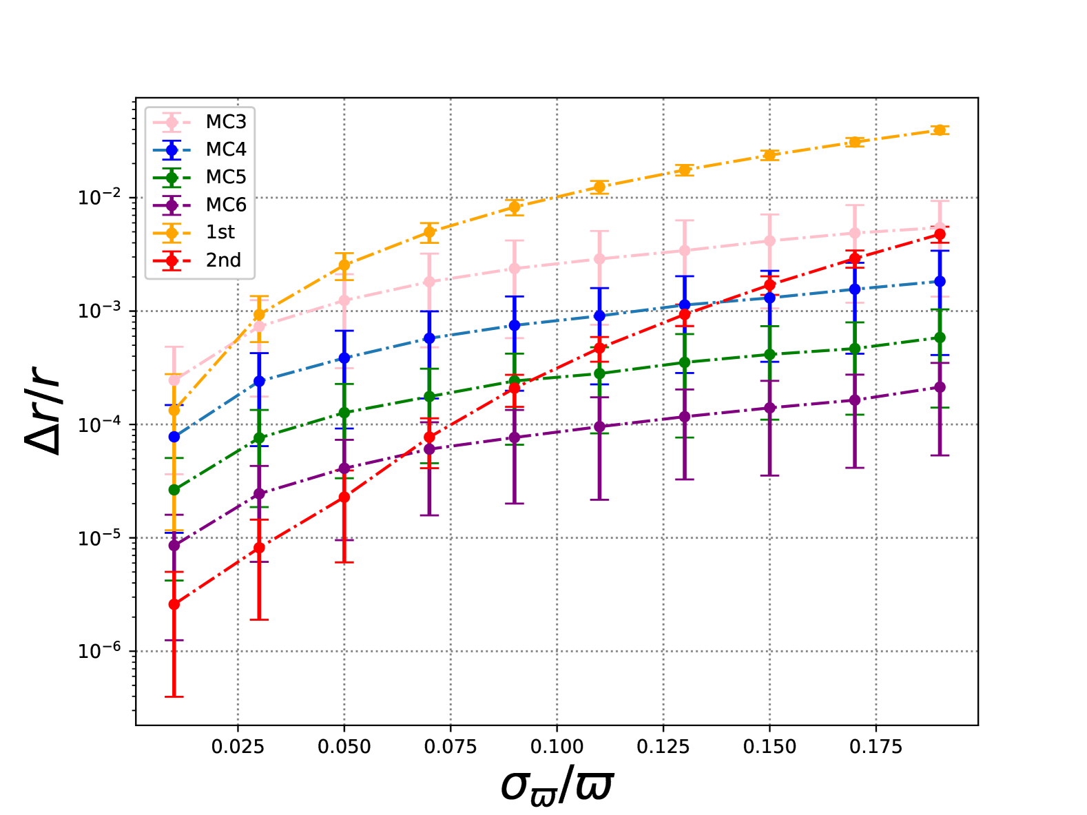
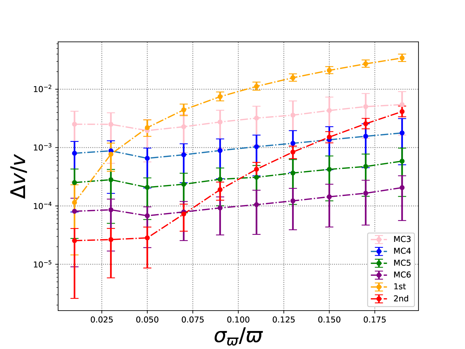
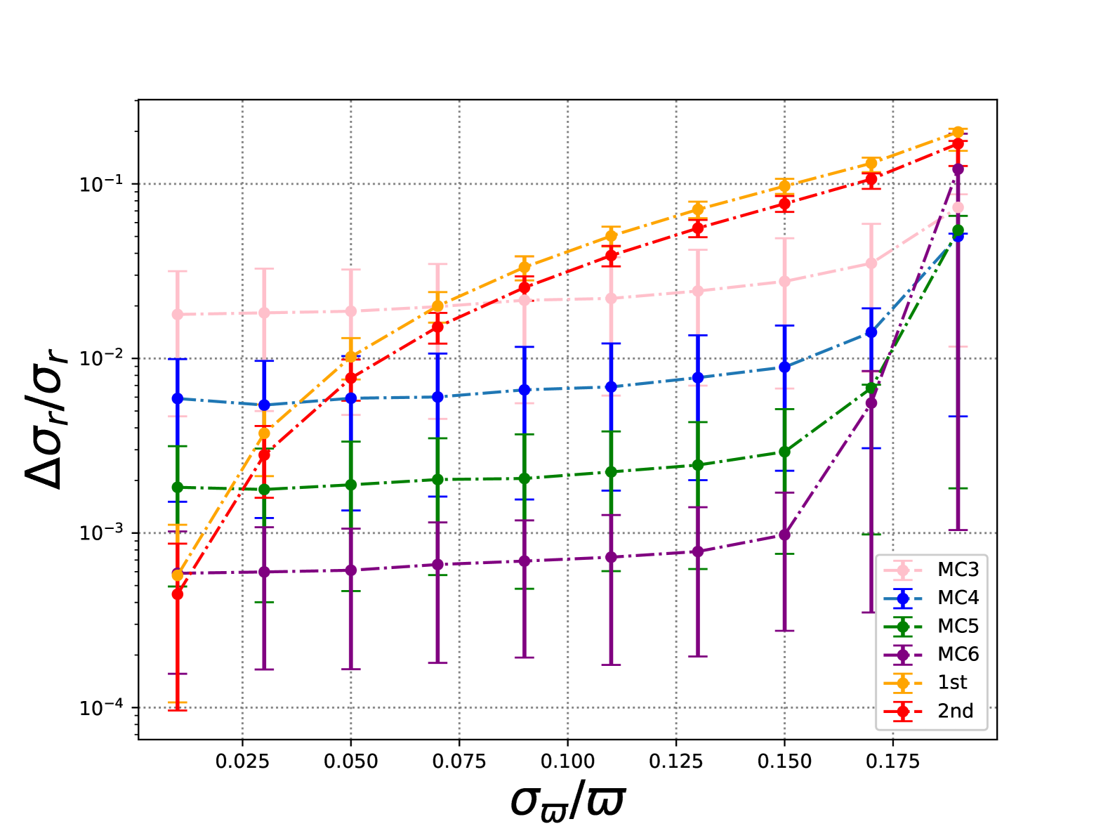
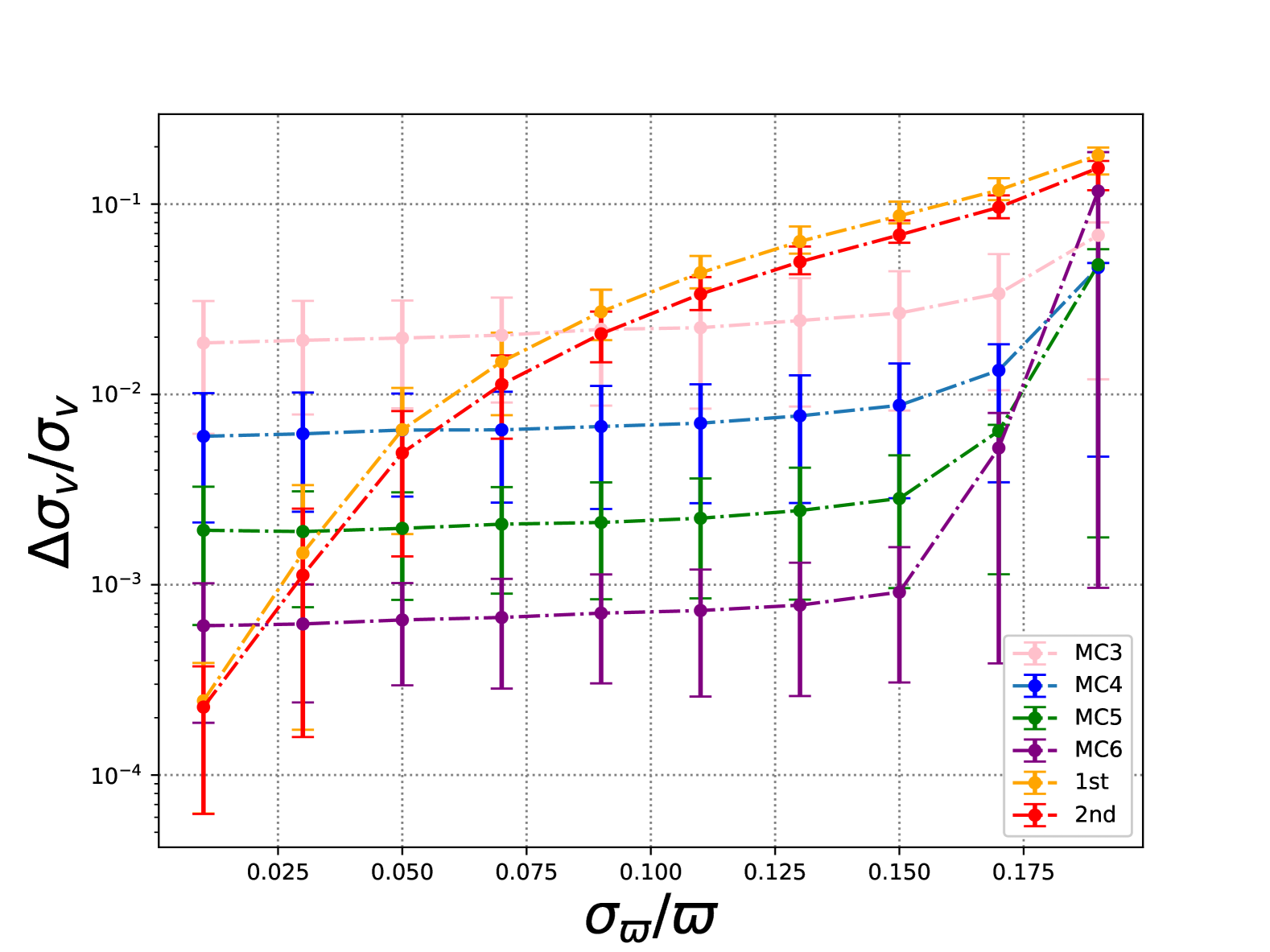
Figure 1: Comparison of first-order ($\rm{1st}$), second-order ($\rm{2nd}$), and MC error propagation methods. Top panels: the fractional deviations of coordinate (left) and velocity (right) propagated with various methods relative to MC7. Bottom panels: the fractional deviations of the variances of coordinate (left) and velocity (right) propagated with various methods relative to $\rm MC7$. The x axis shows the fractional parallax error ($\sigma_{\varpi}/\varpi$) and 10 bins are used to divide the range of $0<\sigma_{\varpi}/\varpi<0.2$. Each dot and error bar respectively represent the average and scatter of the values of 1000 samples. The error bars correspond to quantiles of 16% and 84%.

To investigate the dependence of error propagation on the fractional parallax error, we evenly divide $\sigma_{\varpi}/\varpi$ (with a range of (0, 0.2)) into 10 bins and randomly select 1000 stars from Gaia DR3 for each bin. We employ the linear, second-order, and MC error propagation methods with different sample sizes to transform stars from spherical coordinates and velocities to Cartesian coordinates and velocities in the Equatorial system. We compare the fractional deviations of the mean and variance of various methods relative to MC7 in Fig. 1.

By analyzing the results, we find the following features:

• Propagation of coordinate and velocity: According to the top panels of Fig. 1, the linear error propagation will lead to larger than 1% fractional deviations of mean coordinate and velocity for targets with $\sigma_{\varpi}/\varpi>0.11$. The propagation of mean coordinate and velocity using the second-order error propagation and the MC propagation method with more than 10,000 samples achieves less than 0.2% precision for sources with $0<\sigma_{\varpi}/\varpi<0.15$. The second-order error propagation achieves less than 0.5% precision for sources with $0<\sigma_{\varpi}/\varpi<0.2$.

• Propagation of the variance: As seen from the bottom panels of Fig. 1, the linear and second-order variance propagation can achieve 10% precision for sources with less than 15% fractional parallax error. In contrast, MC method with more than 10,000 samples propagates variance with less than 1% precision for sources with $0<\sigma_{\varpi}/{\varpi}<0.15$. While the second-order error propagation can achieve higher precision for mean transformation than the MC4 method for sources with small fractional parallax error, it fails to propagate variance as precise as MC4. The reason for this is that Gaussian distributions in the spherical coordinate systems are transformed into non-Gaussian distributions in the Cartesian coordinate system. Because the higher moments are not taken into account in calculating the variance of non-Gaussian distributions, the second-order error propagation is less accurate in propagating the variance (and covariance) than propagating the mean.

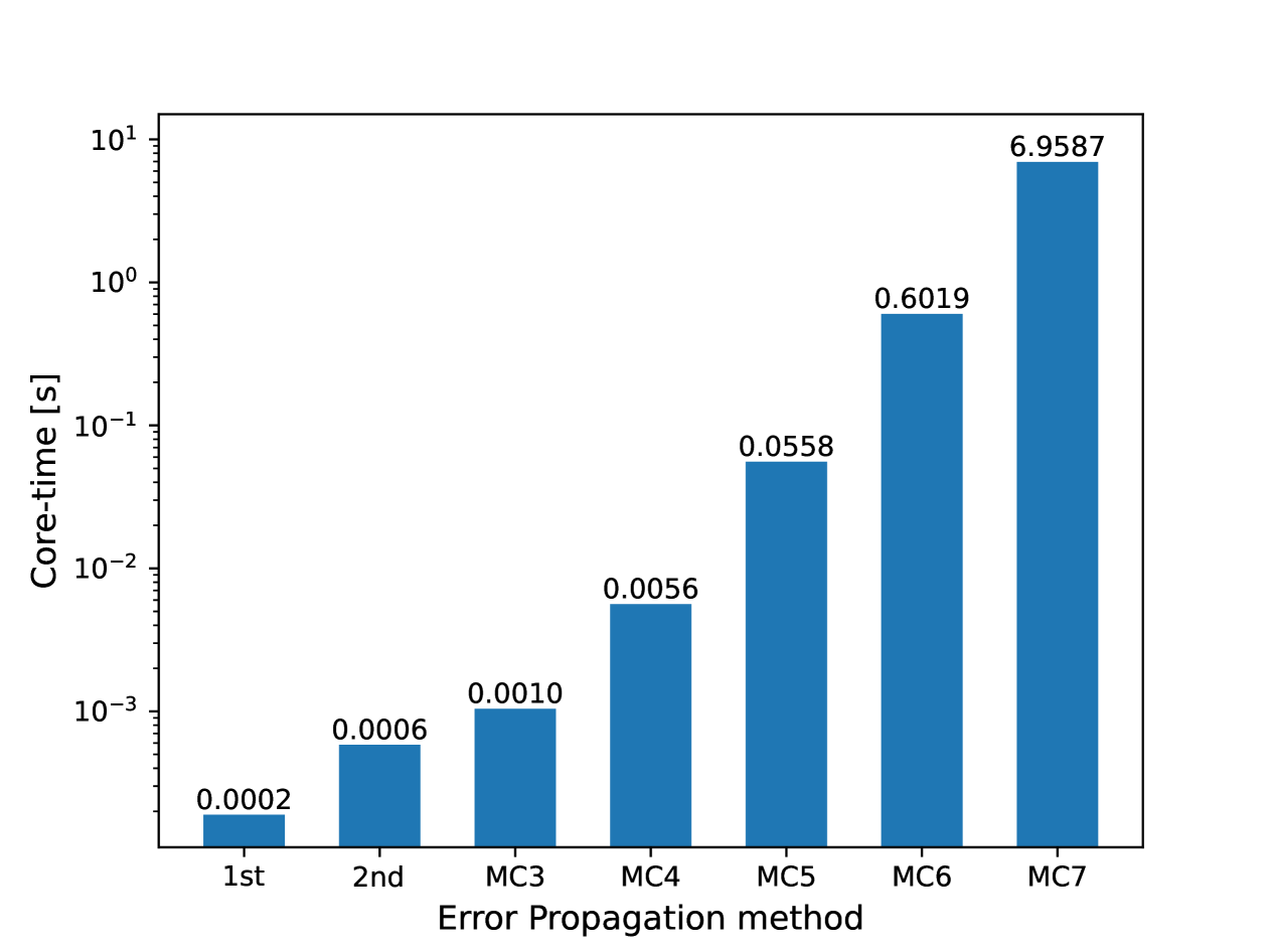
Figure 2: Comparison of the CPU time of the various propagation methods. Each bar in the chart shows a single run time for the equatorial Cartesian coordinate and covariance transformation of the respective propagation method, which is taken as an average of 10,000 runs. The CPU model is Intel(R) Xeon(R) Silver 4210R CPU @ 2.40GHz .

To evaluate the efficiency of various propagation methods, we calculate the computational time of mean and covariance for each method in Fig. 2. The time consumed by MC method is linearly proportional to the number of MC samples. Meanwhile the execution time for second-order error propagation is one order of magnitude lower than that of MC4. Although MC3 requires a comparable amount of time as second-order error propagation, the latter exhibits significantly higher precision in propagation, as illustrated in Fig. 1.

Therefore, considering the efficiency and precision of error propagation, we recommend the second-order error propagation for mean transformation with approximately 0.5% precision and for covariance propagation with 10% precision. If higher precision of variance propagation is needed, we recommend using the MC4 method. Combining the advantages of both methods, we apply the second-order error propagation to convert the means, and employ MC4 to propagate the covariance of astrometric parameters and radial velocities of 30 million Gaia sources with $0<\sigma_{\varpi}/{\varpi}<0.2$ into Cartesian coordinates and velocities in both the Equatorial and Galactic coordinate systems. In this way, the average CPU time required for a single calculation of a set of Cartesian catalog data (including both galactic and equatorial coordinate systems) is only 0.0065 s.

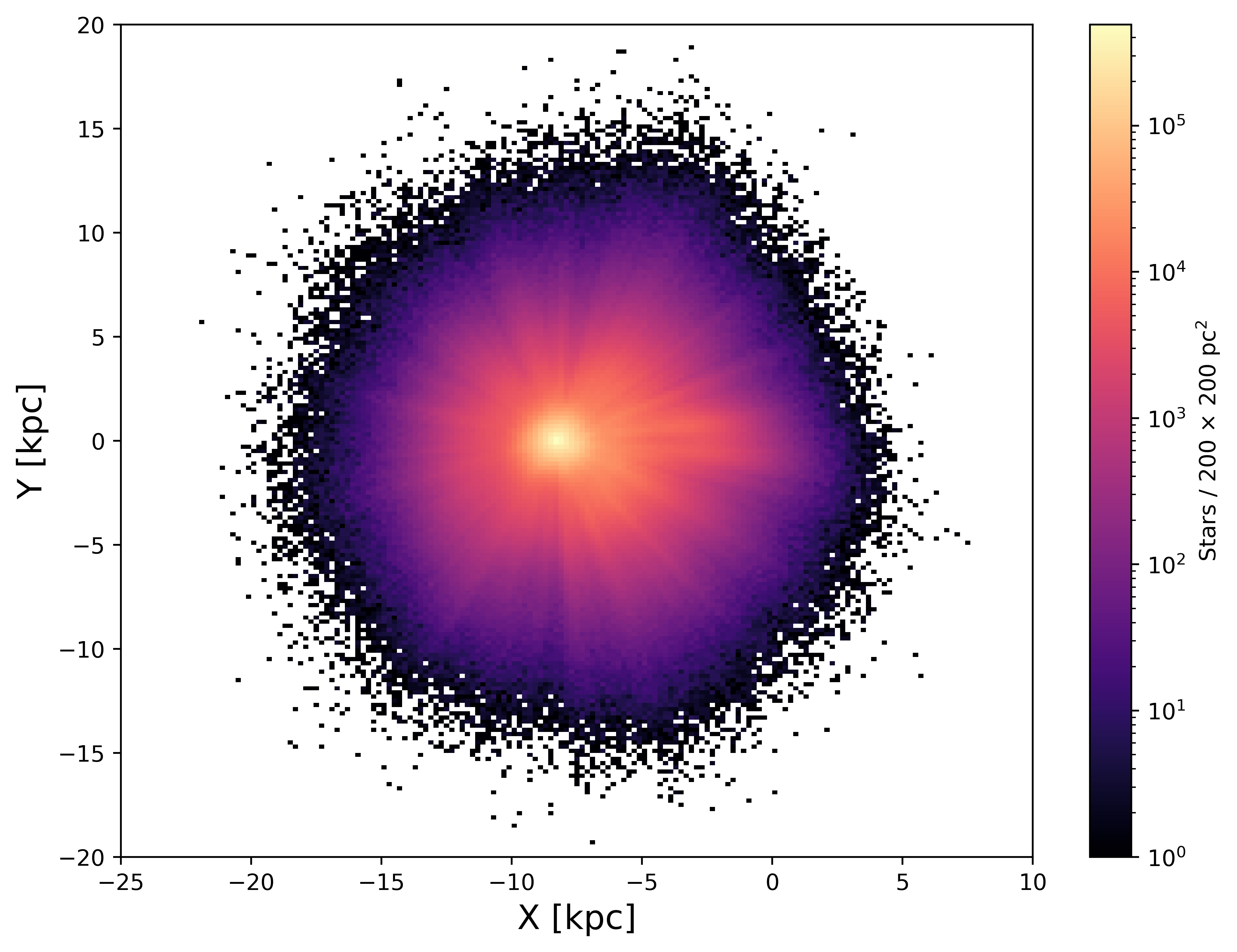
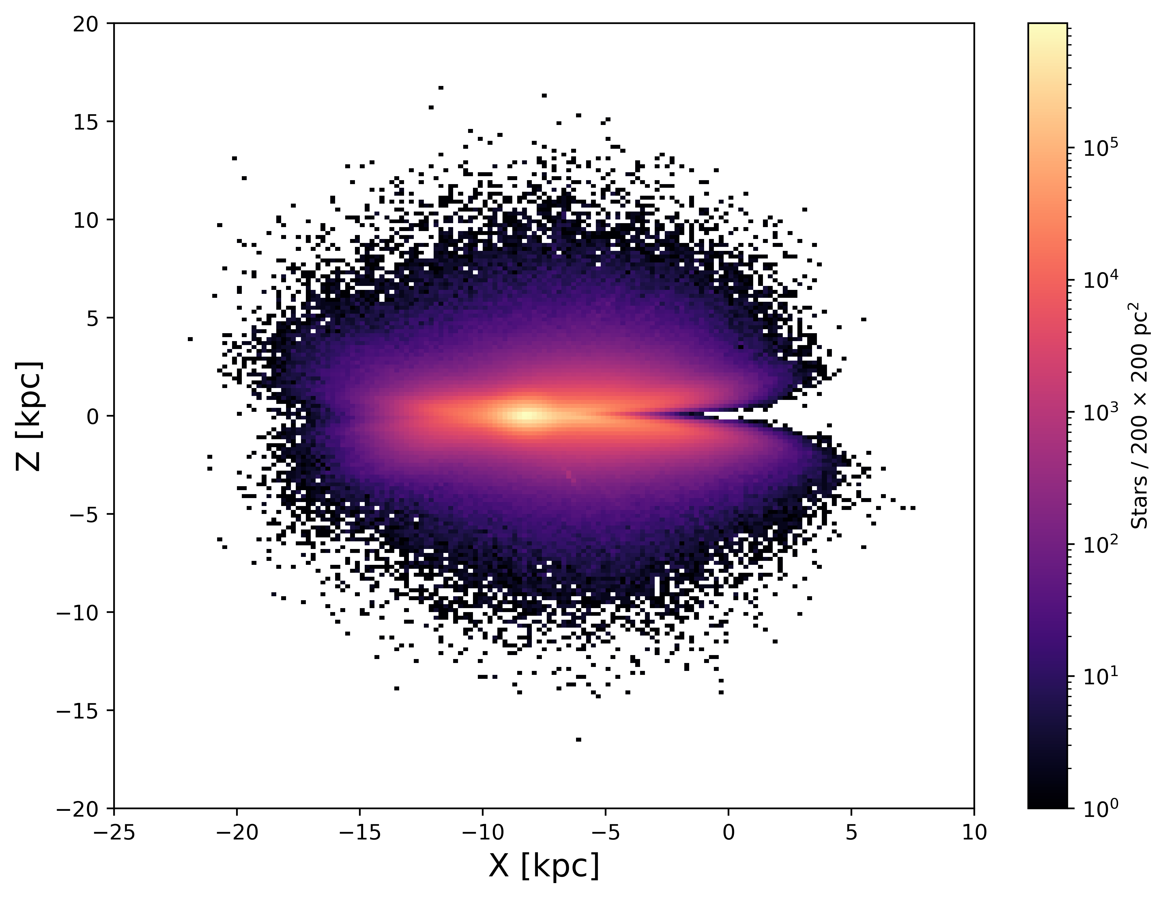
Figure 3: Spatial distributions of stars from our Cartesian catalog (similar to Fig. 2 in Katz, D. et al. (2023)). Left: a face-on view of catalog stars in galactocentric Cartesian coordinates (X, Y). Right: an edge-on view of the same data in galactocentric Cartesian coordinates (X, Z). The Galactic center is at X = Y = 0 kpc, with the Sun positioned at X = -8.277 kpc GRAVITY Collaboration et al. (2022), Y = 0 kpc, and Z = 20.8 pc Bennett & Bovy (2018). The Milky Way is viewed from the Galactic north pole and rotates clockwise, with the Z-axis positive towards the north pole. The stars are binned by a 200 pc $\times$ 200 pc grid.

Fig. 3 shows the galactocentric Cartesian coordinate distribution of stars. The figure displays a sample of 31,066,855 stars from Gaia DR3 with radial velocity, where the parallax satisfies $0<\sigma_{\varpi}/\varpi<0.2$ and duplicated sources are removed. Although the face-on view (XY plane) is similar to Fig. 2 in Katz, D. et al. (2023), Fig. 3 doesn’t have elongated features in face-on and edge-on views, because the catalog doesn’t contain Large and Small Magellanic Cloud stars due to their fractional parallax errors larger than 20% (as discussed in Bailer-Jones et al. (2021)).

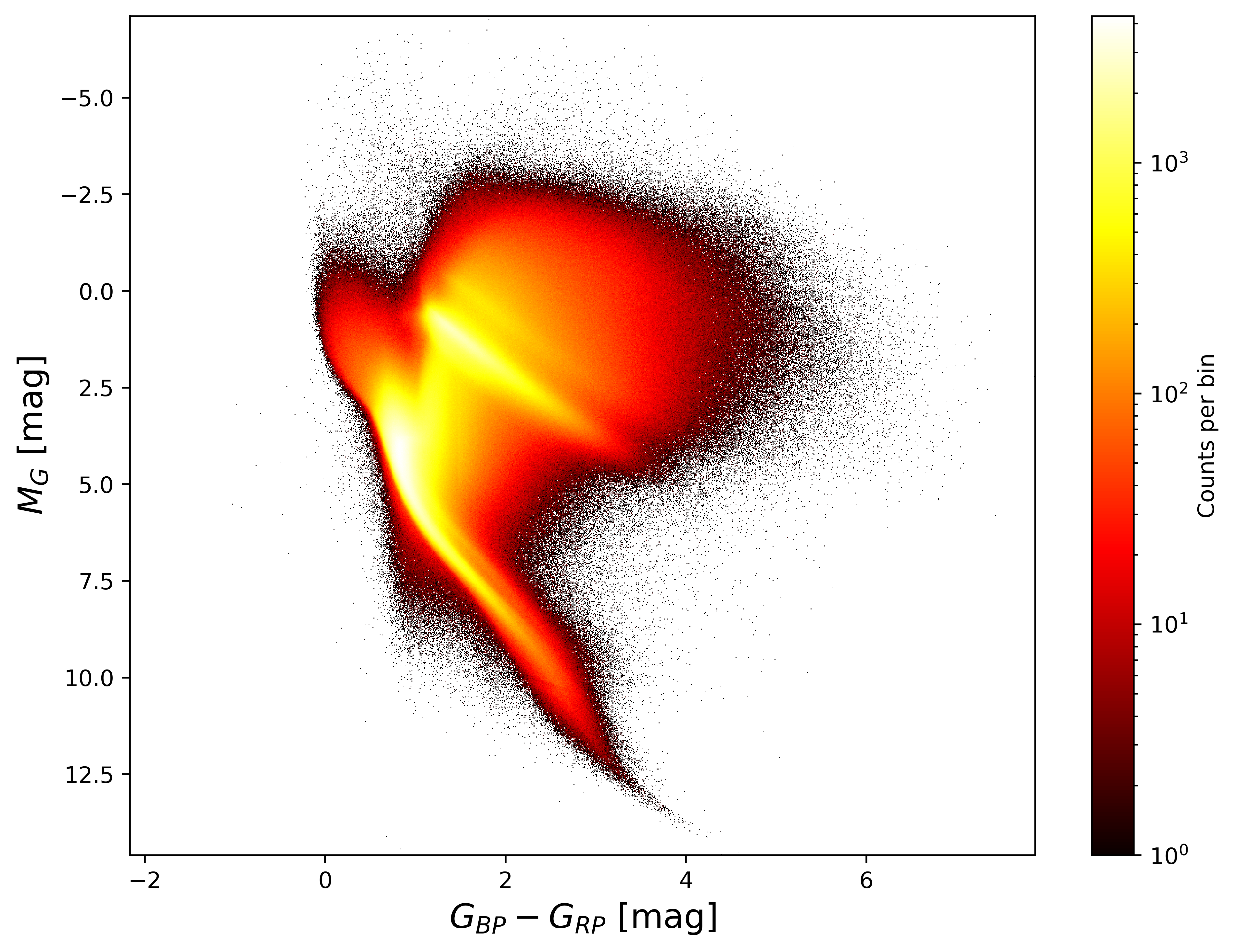
Figure 4: Hertzsprung-Russell diagram of the Cartesian catalog. The colorbar represents the frequency of stars in Gaia DR3 with radial velocity and fractional parallax error satisfying $0<\sigma_{\varpi}/\varpi<0.2$.

The Hertzsprung-Russell (HR) diagram of the Cartesian catalog is shown in Fig. 4, which includes only data with $M_{G}$ and $G_{BP}-G_{RP}$. The figure shows that the Cartesian catalog contains stars with absolute magnitudes ranging from 15 to -5, including a large number of red giants and main-sequence stars, but no white dwarfs. The spectroscopic pipeline of Gaia lacks an appropriate template for white dwarfs, and the mismatch between the observed spectra and the templates can lead to significant systematic errors in radial velocity measurements (Katz, D. et al. 2023). Consequently, white dwarfs lack radial velocity data and are not included in this catalog.

The Cartesian catalog in Appendix A contains the mean of Cartesian coordinates determined by the second-order error propagation and the covariance of Cartesian coordinates determined by the MC4 method. We also include the values of transversal velocity and distance in the catalog.

5 Discussion and conclusion

In our study based on Gaia DR3 data, we compare various error propagation methods and identify second-order error propagation as the most efficient for achieving nearly 0.5% precision in propagating mean coordinates and velocities. Linear propagation commonly used fails to achieve 1% precision in coordinate and velocity mean when the fractional parallax error exceeds 10%.

However, the precision of second-order error propagation for variance is inferior to that for mean transformation. This discrepancy arises due to the nonlinear coordinate transformation introducing non-Gaussian errors in new coordinate systems. Although the MC4 method is about 10 times more computationally expensive than the second-order method, it achieves more accurate covariance propagation than the latter. Therefore, for propagating covariance with nearly 1% precision, we suggest employing the MC propagation method with a minimum of 10,000 samples.

Balancing efficiency and precision, we employ second-order error propagation for the mean values of 31,129,169 Gaia sources with radial velocity and fractional parallax error below 20%, and utilize MC4 for covariance conversion. We present the Cartesian coordinates, velocities, and their covariances in both Equatorial and Galactic coordinate systems. This catalog offers highly precise mean coordinates and velocities, facilitating applications such as the accurate integration of stellar orbits and the study of wide binaries.

Subsequent investigations into precise error propagation should address the non-Gaussian nature of errors and incorporate higher moments, including skewness and kurtosis, in the propagation process. Advanced techniques such as the Kalman and unscented filters (mentioned in Section 1) may offer more efficient and accurate results for error propagation in stellar motions.

Data availability

The complete data in Appendix 1 will be available on Vizier and the source code could be found on github (https://github.com/LuyaoZhang-sjtu/GaiaDR3-error-propagation).

Appendix A Data sample

Table 1: Examples of the catalog of coordinates and velocities in Equatorial and Galactic coordinate systems based on second-order error propagation and their covariances based on MC4. The correlation coefficients between Cartesian coordinates are explained in section D.

Gaia DR3 source_id	r_eqt	r_eqt_error	vt_eqt	vt_eqt_error	x_eqt	x_eqt_error	x_gal	x_gal_error	y_eqt	y_eqt_error
	[$\,\rm{pc}$]	[$\,\rm{pc}$]	[$\,\rm{km}\,\rm{s}^{-1}$]	[$\,\rm{km}\,\rm{s}^{-1}$]	[$\,\rm{pc}$]	[$\,\rm{pc}$]	[$\,\rm{pc}$]	[$\,\rm{pc}$]	[$\,\rm{pc}$]	[$\,\rm{pc}$]
200030787485939968	647.031553	8.665063	20601.543326	287.025171	134.532389	1.801530	-624.933163	8.368510	475.844692	6.372059
243131265338696960	1467.466212	44.418498	41853.421674	1250.012167	627.700148	18.996902	-1231.688678	37.276189	773.748036	23.416938
171961316481695872	2046.674971	86.670104	10185.771205	462.796237	594.034343	25.149937	-1978.215127	83.752711	1606.417789	68.011736
55616669682429568	255.495582	15.084233	11847.245619	815.448020	159.844142	9.448656	-206.101795	12.183024	183.827943	10.866379
159237767925095808	4389.670253	396.858380	14210.820602	1362.759362	1334.125320	120.634047	-4240.114346	383.398880	3524.523748	318.693871
228161685104953472	3157.411196	351.706897	41874.578692	4738.891542	937.323592	104.518807	-2955.617920	329.574186	2165.808759	241.504375
176758313916240384	3546.819656	457.715455	34882.973858	4490.540202	1146.974741	148.282909	-3352.638332	433.434972	2589.499195	334.775004
110527723485651328	5401.092771	817.497730	62859.597739	9489.374298	3252.277495	493.056627	-4472.803410	678.092618	3735.441241	566.305938
266107794183243392	3948.204353	707.938159	30907.151439	5587.757422	539.050640	97.015368	-3559.286905	640.580872	2298.168517	413.611724
199834524659602560	6300.091255	1130.725447	47534.769063	8538.895743	1533.934200	276.429692	-6018.874085	1084.658983	4569.422215	823.453820

y_gal	y_gal_error	z_eqt	z_eqt_error	z_gal	z_gal_error	vx_eqt	vx_eqt_error	vx_gal	vx_gal_error	vy_eqt	vy_eqt_error
[$\,\rm{pc}$]	[$\,\rm{pc}$]	[$\,\rm{pc}$]	[$\,\rm{pc}$]	[$\,\rm{pc}$]	[$\,\rm{pc}$]	[$\,\rm{km}\,\rm{s}^{-1}$]	[$\,\rm{km}\,\rm{s}^{-1}$]	[$\,\rm{km}\,\rm{s}^{-1}$]	[$\,\rm{km}\,\rm{s}^{-1}$]	[$\,\rm{km}\,\rm{s}^{-1}$]	[$\,\rm{km}\,\rm{s}^{-1}$]
166.559433	2.230405	417.353424	5.588799	-20.676366	0.276878	-15.519831	1.084849	55.609456	5.022529	-32.056864	3.828528
770.979814	23.333160	1077.687511	32.615452	-206.487278	6.249192	-12.399473	3.329478	-7.575050	6.562881	27.484758	4.250384
416.508218	17.633923	1121.275231	47.472006	-322.333480	13.646798	-14.309175	0.556296	14.814779	1.215064	-9.772316	1.004909
53.973826	3.190484	75.993056	4.492078	-140.451711	8.302337	28.158682	3.147573	-20.936957	4.014908	15.095567	3.607896
771.830412	69.790315	2249.637881	203.416364	-829.901657	75.041223	-2.715690	0.974283	-23.395144	0.424860	25.014346	0.805159
1062.875886	118.518856	2092.622279	233.343518	-288.077519	32.122864	-8.070650	2.798039	-1.796631	8.596169	22.500453	7.092617
1001.847367	129.520587	2124.552047	274.665820	-539.348314	69.727897	-2.250695	2.588164	51.817585	3.789200	-25.652130	3.466915
1538.102217	233.181668	2132.255005	323.257306	-2589.519802	392.580246	-32.000688	5.176726	44.659904	7.084487	-6.910449	7.502853
1594.456714	286.961546	3146.528012	566.294797	511.837053	92.117616	-21.123758	3.874245	-12.776766	8.054188	20.769009	6.272847
1725.990732	311.040126	4017.062578	723.913302	-404.321664	72.862652	-28.188661	6.384590	-41.533855	3.926764	48.115034	5.407343

vy_gal	vy_gal_error	vz_eqt	vz_eqt_error	vz_gal	vz_gal_error	x_y_eqt_corr	x_y_gal_corr	x_z_eqt_corr	x_z_gal_corr	x_vx_eqt_corr	x_vx_gal_corr
[$\,\rm{km}\,\rm{s}^{-1}$]	[$\,\rm{km}\,\rm{s}^{-1}$]	[$\,\rm{km}\,\rm{s}^{-1}$]	[$\,\rm{km}\,\rm{s}^{-1}$]	[$\,\rm{km}\,\rm{s}^{-1}$]	[$\,\rm{km}\,\rm{s}^{-1}$]
-34.719950	1.363982	-55.304265	3.361144	-5.402112	0.213469	1.0	-1	1.0	1.0	-0.025778	0.007938
-42.669929	4.195569	-32.553917	5.735937	-9.529537	1.173857	1.0	-1	1.0	1.0	-0.029167	0.108153
-11.205423	0.432668	-11.355213	0.701772	9.173458	0.384982	1.0	-1	1.0	1.0	-0.613767	0.089652
16.780904	1.228443	12.828138	1.502041	-21.572986	2.748034	1.0	-1	1.0	1.0	0.167898	-0.092520
-9.850999	1.288472	3.504734	0.731835	-1.000336	0.540765	1.0	-1	1.0	1.0	-0.824537	0.634052
-40.880532	5.207441	-35.989984	6.824120	-13.865027	1.921271	1.0	-1	1.0	1.0	-0.201012	0.159771
-34.919209	2.647298	-60.534173	4.225765	-20.568671	3.899867	1.0	-1	1.0	1.0	0.819537	0.015970
-69.657557	8.532614	-76.199526	8.954340	-5.611040	6.346341	1.0	-1	1.0	1.0	0.026984	0.004039
-26.167317	6.096840	-8.689895	7.205121	10.252069	2.056878	1.0	-1	1.0	-1.0	-0.922549	0.252909
-33.702068	7.640647	2.181059	3.766084	15.922425	3.222852	1.0	-1	1.0	1.0	-0.981286	0.608243

x_vy_eqt_corr	x_vy_gal_corr	x_vz_eqt_corr	x_vz_gal_corr	y_z_eqt_corr	y_z_gal_corr	y_vx_eqt_corr	y_vx_gal_corr	y_vy_eqt_corr	y_vy_gal_corr	y_vz_eqt_corr	y_vz_gal_corr
0.044574	0.187635	-0.066197	0.519949	1.0	-1.0	-0.025778	-0.007938	0.044574	-0.187635	-0.066197	-0.519949
0.264101	0.228089	-0.095608	0.330662	1.0	-1.0	-0.029167	-0.108153	0.264101	-0.228089	-0.095608	-0.330662
0.170093	0.642822	-0.063692	-0.628638	1.0	-1.0	-0.613767	-0.089652	0.170093	-0.642822	-0.063692	0.628638
-0.149765	-0.498075	0.098375	0.103394	1.0	-1.0	0.167898	0.092520	-0.149765	0.498075	0.098375	-0.103394
0.885004	0.924225	-0.872434	-0.489577	1.0	-1.0	-0.824537	-0.634052	0.885004	-0.924225	-0.872434	0.489577
0.479148	0.807361	-0.473696	0.863558	1.0	-1.0	-0.201012	-0.159771	0.479148	-0.807361	-0.473696	-0.863558
0.531466	0.884858	-0.814464	0.967916	1.0	-1.0	0.819537	-0.015970	0.531466	-0.884858	-0.814464	-0.967916
0.613966	0.956273	-0.923856	0.757251	1.0	-1.0	0.026984	-0.004039	0.613966	-0.956273	-0.923856	-0.757251
0.589206	0.811314	-0.285452	-0.695849	1.0	1.0	-0.922549	-0.252909	0.589206	-0.811314	-0.285452	0.695849
0.894921	0.988857	-0.820157	-0.952284	1.0	-1.0	-0.981286	-0.608243	0.894921	-0.988857	-0.820157	0.952284

z_vx_eqt_corr	z_vx_gal_corr	z_vy_eqt_corr	z_vy_gal_corr	z_vz_eqt_corr	z_vz_gal_corr	vx_vy_eqt_corr	vx_vy_gal_corr	vx_vz_eqt_corr	vx_vz_gal_corr	vy_vz_eqt_corr	vy_vz_gal_corr
-0.025778	0.007938	0.044574	0.187635	-0.066197	0.519949	0.994716	-0.979444	0.996427	0.786199	0.993584	-0.674004
-0.029167	0.108153	0.264101	0.228089	-0.095608	0.330662	0.954551	-0.942633	0.995686	0.960283	0.934157	-0.830872
-0.613767	0.089652	0.170093	0.642822	-0.063692	-0.628638	0.501601	-0.504215	0.666283	0.433038	0.921174	-0.798679
0.167898	-0.092520	-0.149765	-0.498075	0.098375	0.103394	0.941081	-0.794564	0.969693	0.968901	0.952575	-0.889424
-0.824537	0.634052	0.885004	0.924225	-0.872434	-0.489577	-0.842508	0.664945	0.742314	-0.497302	-0.817323	-0.592257
-0.201012	0.159771	0.479148	0.807361	-0.473696	0.863558	0.745502	-0.447692	0.939536	0.563474	0.543182	0.438997
0.819537	0.015970	0.531466	0.884858	-0.814464	0.967916	0.844144	-0.406029	-0.402566	0.160099	0.040033	0.785306
0.026984	0.004039	0.613966	0.956273	-0.923856	0.757251	0.791982	-0.279000	0.344724	0.640388	-0.271265	0.540706
-0.922549	-0.252909	0.589206	-0.811314	-0.285452	0.695849	-0.299324	-0.343299	0.547329	-0.697581	0.590029	-0.254861
-0.981286	0.608243	0.894921	0.988857	-0.820157	-0.952284	-0.827424	0.514619	0.863911	-0.535484	-0.505155	-0.953220

Appendix B Transformation from Equatorial to Galactic coordinate system

The following relationship exists between coordinates in Equatorial and Galactic coordinate systems:

$$\cos{b}\cos{(l_{\rm NEP}-l)}=\cos{(\delta_{\rm NGP})}\sin{\delta}-\sin{(\delta_{\rm NGP})}\cos{\delta}\cos{(\alpha-\alpha_{\rm NGP})}~,$$ (16)

$$\cos{b}\sin{(l_{\rm NEP}-l)}=\cos{\delta}\sin{(\alpha-\alpha_{\rm NGP})}~,$$

$$\sin{b}=\sin{(\delta_{\rm NGP})}\sin{\delta}+\cos{(\delta_{\rm NGP})}\cos{\delta}\cos{(\alpha-\alpha_{\rm NGP})}~.$$

During the calculation process, the galactic pole coordinates are consistent with those in the Python package astropy, where

$$l_{\rm NGP}=122.93192526\degree~,$$ (17)

$$\alpha_{\rm NGP}=192.85947789\degree~,$$

$$\delta_{\rm NGP}=27.12825241\degree~.$$

The position coordinate matrices of coordinates in Equatorial ($\rm eqt$) and Galactic ($\rm gal$) coordinate systems are defined as follows:

$$\bm{P}^{\rm eqt}=\begin{bmatrix}x^{\rm eqt}\\ y^{\rm eqt}\\ z^{\rm eqt}\\ \end{bmatrix}=\begin{bmatrix}\cos{\delta}\cos{\alpha}\\ \cos{\delta}\sin{\alpha}\\ \sin{\delta}\\ \end{bmatrix},\bm{P}^{\rm gal}=\begin{bmatrix}x^{\rm gal}\\ y^{\rm gal}\\ z^{\rm gal}\\ \end{bmatrix}=\begin{bmatrix}\cos{b}\cos{l}\\ \cos{b}\sin{l}\\ \sin{b}\\ \end{bmatrix}~.$$ (18)

By separating the position coordinate matrices from the equations LABEL:eq:gal, we extract the rotation matrix $\bm{R}$:

$$\bm{R}=\begin{bmatrix}-\sin{(\delta_{\rm NGP})}\cos{(\alpha_{\rm NGP})}&-\sin{(\delta_{\rm NGP})}\sin{(\alpha_{\rm NGP})}&\cos{(\delta_{\rm NGP})}\\ -\sin{(\alpha_{\rm NGP})}&\cos{(\alpha_{\rm NGP})}&0\\ \cos{(\delta_{\rm NGP})}\cos{(\alpha_{\rm NGP})}&\cos{(\delta_{\rm NGP})}\sin{(\alpha_{\rm NGP})}&\sin{(\delta_{\rm NGP})}\end{bmatrix}~.$$ (19)

The velocity coordinate matrix $\bm{V}^{\rm eqt}$ is the derivative of the equatorial position coordinate matrix with respect to time. Therefore, for both position and velocity propagation, it just needs to multiply by the rotation matrix as follows:

$$\bm{P}^{\rm gal}=\bm{R}\bm{P}^{\rm eqt}~,$$ (20)

$$\bm{V}^{\rm gal}=\bm{R}\dot{\bm{P}}^{\rm eqt}=\bm{R}\bm{V}^{\rm eqt}~.$$

Hence, the linear and non-linear calculation of galactic coordinates only depends on the matrices of Cartesian coordinates $\bm{P}$ and velocities $\bm{V}$ in the Equatorial coordinate system. The galactic variance-covariance matrix is calculated as follows:

$$\bm{C}^{\rm gal}_{\rm car}=\bm{R}\bm{C}^{\rm eqt}_{\rm car}\bm{R}^{T}~.$$ (21)

Appendix C Jacobian matrix

The elements of the Jacobian matrix are given below, where $\rm{A}=1\,\rm{AU}$:

$$\ \bm{J}_{11}=\frac{\partial\rm x}{\partial\alpha}=-\frac{\rm{A}\sin{\alpha}\cos{\delta}}{\varpi}$$ (22)

$$\ \bm{J}_{12}=\frac{\partial\rm x}{\partial\delta}=-\frac{\rm{A}\cos{\alpha}\sin{\delta}}{\varpi}$$ (23)

$$\ \bm{J}_{13}=\frac{\partial\rm x}{\partial\varpi}=-\frac{\rm{A}\cos{\alpha}\cos{\delta}}{\varpi^{2}}$$ (24)

$$\bm{J}_{14}=\frac{\partial\rm x}{\partial\mu_{\alpha^{*}}}=0$$ (25)

$$\bm{J}_{15}=\frac{\partial\rm x}{\partial\mu_{\delta}}=0$$ (26)

$$\bm{J}_{16}=\frac{\partial\rm x}{\partial{v_{r}}}=0$$ (27)

$$\bm{J}_{21}=\frac{\partial\rm y}{\partial\alpha}=\frac{\rm{A}\cos{\alpha}\cos{\delta}}{\varpi}$$ (28)

$$\bm{J}_{22}=\frac{\partial\rm y}{\partial\delta}=-\frac{\rm{A}\sin{\alpha}\sin{\delta}}{\varpi}$$ (29)

$$\bm{J}_{23}=\frac{\partial\rm y}{\partial\varpi}=-\frac{\rm{A}\sin{\alpha}\cos{\delta}}{\varpi^{2}}$$ (30)

$$\bm{J}_{24}=\frac{\partial\rm y}{\partial\mu_{\alpha^{*}}}=0$$ (31)

$$\bm{J}_{25}=\frac{\partial\rm y}{\partial\mu_{\delta}}=0$$ (32)

$$\bm{J}_{26}=\frac{\partial\rm y}{\partial{v_{r}}}=0$$ (33)

$$\bm{J}_{31}=\frac{\partial\rm z}{\partial\alpha}=0$$ (34)

$$\bm{J}_{32}=\frac{\partial\rm z}{\partial\delta}=\frac{\rm{A}\cos{\delta}}{\varpi}$$ (35)

$$\bm{J}_{33}=\frac{\partial\rm z}{\partial\varpi}=-\frac{\rm{A}\sin{\delta}}{\varpi^{2}}$$ (36)

$$\bm{J}_{34}=\frac{\partial\rm z}{\partial\mu_{\alpha^{*}}}=0$$ (37)

$$\bm{J}_{35}=\frac{\partial\rm z}{\partial\mu_{\delta}}=0$$ (38)

$$\bm{J}_{36}=\frac{\partial\rm z}{\partial{v_{r}}}=0$$ (39)

$$\bm{J}_{41}=\frac{\partial\rm v_{x}}{\partial\alpha}=-v_{r}\sin{\alpha}\cos{\delta}+\frac{\rm{A}\mu_{\delta}\sin{\alpha}\sin{\delta}}{\varpi}-\frac{\rm{A}\mu_{\alpha^{*}}\cos{\alpha}}{\varpi}$$ (40)

$$\bm{J}_{42}=\frac{\partial\rm v_{x}}{\partial\delta}=-v_{r}\cos{\alpha}\sin{\delta}-\frac{\rm{A}\mu_{\delta}\cos{\alpha}\cos{\delta}}{\varpi}$$ (41)

$$\bm{J}_{43}=\frac{\partial\rm v_{x}}{\partial\varpi}=\frac{\rm{A}\mu_{\delta}\cos{\alpha}\sin{\delta}}{\varpi^{2}}+\frac{\rm{A}\mu_{\alpha^{*}}\sin{\alpha}}{\varpi^{2}}$$ (42)

$$\bm{J}_{44}=\frac{\partial\rm v_{x}}{\partial\mu_{\alpha^{*}}}=-\frac{\rm{A}\sin{\alpha}}{\varpi}$$ (43)

$$\bm{J}_{45}=\frac{\partial\rm v_{x}}{\partial\mu_{\delta}}=-\frac{\rm{A}\cos{\alpha}\sin{\delta}}{\varpi}$$ (44)

$$\bm{J}_{46}=\frac{\partial\rm v_{x}}{\partial v_{r}}=\cos{\alpha}\cos{\delta}$$ (45)

$$\bm{J}_{51}=\frac{\partial\rm v_{y}}{\partial\alpha}=v_{r}\cos{\alpha}\cos{\delta}-\frac{\rm{A}\mu_{\delta}\cos{\alpha}\sin{\delta}}{\varpi}-\frac{\rm{A}\mu_{\alpha^{*}}\sin{\alpha}}{\varpi}$$ (46)

$$\bm{J}_{52}=\frac{\partial\rm v_{y}}{\partial\delta}=-v_{r}\sin{\alpha}\sin{\delta}-\frac{\rm{A}\mu_{\delta}\sin{\alpha}\cos{\delta}}{\varpi}$$ (47)

$$\bm{J}_{53}=\frac{\partial\rm v_{y}}{\partial\varpi}=\frac{\rm{A}\mu_{\delta}\sin{\alpha}\sin{\delta}}{\varpi^{2}}-\frac{\rm{A}\mu_{\alpha^{*}}\cos{\alpha}}{\varpi^{2}}$$ (48)

$$\bm{J}_{54}=\frac{\partial\rm v_{y}}{\partial\mu_{\alpha^{*}}}=\frac{\rm{A}\cos{\alpha}}{\varpi}$$ (49)

$$\bm{J}_{55}=\frac{\partial\rm v_{y}}{\partial\mu_{\delta}}=-\frac{\rm{A}\sin{\alpha}\sin{\delta}}{\varpi}$$ (50)

$$\bm{J}_{56}=\frac{\partial\rm v_{y}}{\partial v_{r}}=\sin{\alpha}\cos{\delta}$$ (51)

$$\bm{J}_{61}=\frac{\partial\rm v_{z}}{\partial\alpha}=0$$ (52)

$$\bm{J}_{62}=\frac{\partial\rm v_{z}}{\partial\delta}=v_{r}\cos{\delta}-\frac{\rm{A}\mu_{\delta}\sin{\delta}}{\varpi}$$ (53)

$$\bm{J}_{63}=\frac{\partial\rm v_{z}}{\partial\varpi}=-\frac{\rm{A}\mu_{\delta}\cos{\delta}}{\varpi^{2}}$$ (54)

$$\bm{J}_{64}=\frac{\partial\rm v_{z}}{\partial\mu_{\alpha^{*}}}=0$$ (55)

$$\bm{J}_{65}=\frac{\partial\rm v_{z}}{\partial\mu_{\delta}}=\frac{\rm{A}\cos{\delta}}{\varpi}$$ (56)

$$\bm{J}_{66}=\frac{\partial\rm v_{z}}{\partial v_{r}}=\sin{\delta}$$ (57)

Appendix D Correlation coefficient

In the Eq. 5, the correlation coefficient of $x$ and $y$ is:

$$\bm{k}_{\rm xy}=\frac{\sigma_{xy}}{\sigma_{x}\sigma_{y}}=\frac{\sum_{j=1}^{6}\sum_{i=1}^{6}\frac{\partial{\rm{F_{x}}}}{\partial{b_{i}}}\frac{\partial{\rm{F_{y}}}}{\partial{b_{j}}}\sigma_{b_{i}}\sigma_{b_{j}}k_{ij}}{\sqrt{\sum_{i=1}^{6}(\frac{\partial{\rm{F_{x}}}}{\partial{b_{i}}}\sigma_{b_{i}})^{2}}\sqrt{\sum_{j=1}^{6}(\frac{\partial{\rm{F_{y}}}}{\partial{b_{j}}}\sigma_{b_{j}})^{2}}}~.$$ (58)

This equation for $x$ and $y$ is only related to $\alpha$, $\delta$ and $r$ (see Eq. 2, and $r=\frac{\rm A}{\varpi}~$, where $\rm{A}=1\,\rm{AU}$), so $b_{i},b_{j}=\alpha,\delta,\varpi$. Because $\sigma_{\alpha},\sigma_{\delta}$ is too small compared to the values of $\alpha$ and $\delta$, as $\sigma_{\alpha},\sigma_{\delta}$ approaches 0, the correlation coefficient of $x$ and $y$ simplifies to:

$$\bm{k}_{\rm xy}\approx\frac{\frac{\partial{\rm{F_{x}}}}{\partial{\varpi}}\frac{\partial{\rm{F_{y}}}}{\partial{\varpi}}\sigma_{\varpi}^{2}}{(\frac{\partial{\rm{F_{x}}}}{\partial{\varpi}}\sigma_{\varpi})(\frac{\partial{\rm{F_{y}}}}{\partial{\varpi}}\sigma_{\varpi})}~.$$ (59)

The same is true for the correlation coefficients $k_{xz}$ and $k_{yz}$. As a result, there are many $x$, $y$ and $z$ correlation coefficients approaching $\pm~1$ in the resulting Cartesian catalog.

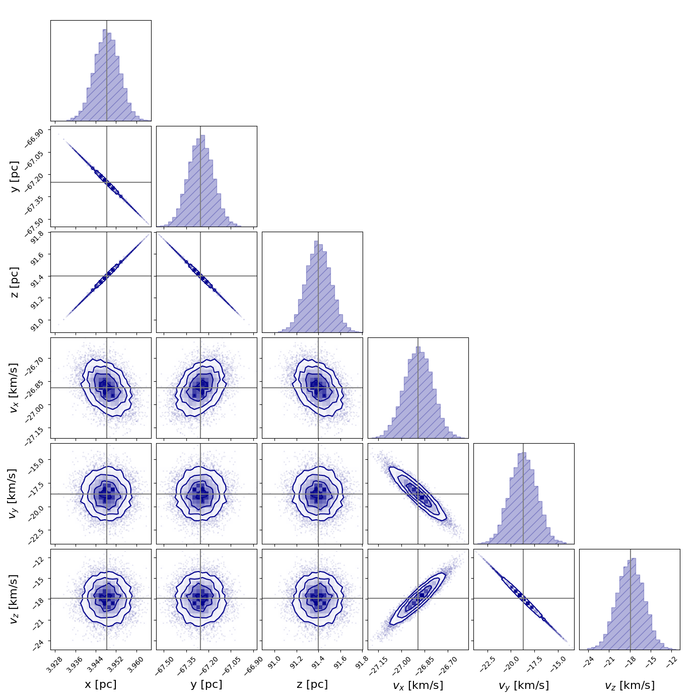
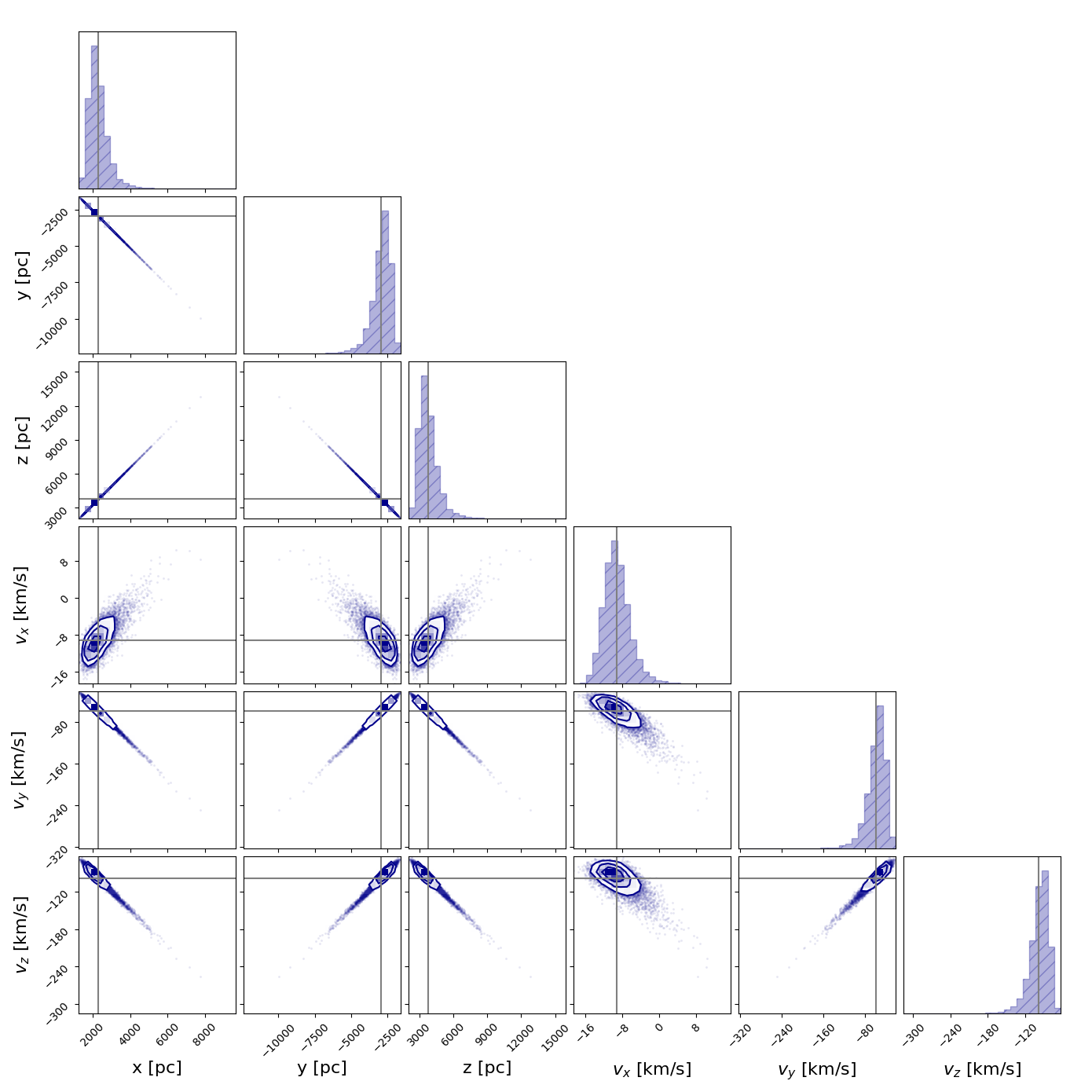
Figure 5: Cornerplots showing the distributions of the MC4 method. The MC4 distribution for the equatorial Cartesian coordinates for Gaia DR3 2149392370122774528 (top) and Gaia DR3 2070799897454308224 (bottom), which have fractional parallax errors of 0.001 and 0.199, respectively. Blue dots represent MC4 samples while the contours represent 0.5, 1, 1.5 and 2 $\sigma$ confidence levels. The mean is shown by horizontal and vertical grey lines.

Fig. 5 shows the sample distributions from the MC4 method. For Gaia DR3 2149392370122774528 and Gaia DR3 2070799897454308224, the correlation coefficient between $x$, $y$, and $z$ is approximately $\pm~1$, regardless of fractional parallax errors. Higher fractional parallax errors lead to a more skewed distribution of the six-dimensional parameters, indicating the significant impact of fractional parallax error on higher-order moments.

Appendix E Acronyms and variables

Table 2: Glossary of main acronyms and variables.

Symbol	Definition
$\alpha$	Right ascension
$\delta$	Declination
$\varpi$	Parallax
$\mu_{\alpha^{*}}$	Proper motion in Right ascension, $\mu_{\alpha^{*}}=\mu_{\alpha}\cos{\delta}$
$\mu_{\delta}$	Proper motion in Declination
$v_{r}$	radial velocity
$k_{ij}$	Correlation coefficient between i and j
$\bm{C}$	Variance-Covariance matrix
$\bm{H}$	Hessian matrix
tr($\bm{I}$)	Trace of matrix $\bm{I}$
$\rm MCi$	MC error propagation method in sample of $10^{i}$
$\rm{1st}$	Linear (first-order) propagation
$\rm{2nd}$	Second-order error propagation
$r$	distance
$\sigma_{i}$	Error (uncertainty) of i
$M_{G}$	Absolute magnitude in the G-band
$G_{BP}-G_{RP}$	BP-RP colour
$l_{\rm NGP}$	Galactic longitude of the north galactic pole
$l_{\rm NEP}$	Galactic longitude of the north equatorial pole
$b$	Galactic latitude
$\rm car$	Cartesian coordinates
$\rm sph$	Spherical coordinates
$\rm eqt$	Equatorial coordinate system
$\rm gal$	Galactic coordinate system

References

- Astraatmadja & Bailer-Jones (2016) Astraatmadja, T. L., & Bailer-Jones, C. A. L. 2016, ApJ, 832, 137
- Bailer-Jones (2015) Bailer-Jones, C. A. L. 2015, PASP, 127, 994
- Bailer-Jones et al. (2018) Bailer-Jones, C. A. L., Farnocchia, D., Meech, K. J., et al. 2018, The Astronomical Journal, 156, 205
- Bailer-Jones et al. (2021) Bailer-Jones, C. A. L., Rybizki, J., Fouesneau, M., Demleitner, M., & Andrae, R. 2021, AJ, 161, 147
- Bailer-Jones et al. (2018) Bailer-Jones, C. A. L., Rybizki, J., Fouesneau, M., Mantelet, G., & Andrae, R. 2018, AJ, 156, 58
- Bennett & Bovy (2018) Bennett, M., & Bovy, J. 2018, Monthly Notices of the Royal Astronomical Society, 482, 1417
- Bonaca et al. (2014) Bonaca, A., Geha, M., Küpper, A. H. W., et al. 2014, ApJ, 795, 94
- Bovy (2014) Bovy, J. 2014, ApJ, 795, 95
- Bovy et al. (2016) Bovy, J., Bahmanyar, A., Fritz, T. K., & Kallivayalil, N. 2016, ApJ, 833, 31
- Bromley et al. (2018) Bromley, B. C., Kenyon, S. J., Brown, W. R., & Geller, M. J. 2018, ApJ, 868, 25
- Butkevich & Lindegren (2014) Butkevich, A. G., & Lindegren, L. 2014, A&A, 570, A62
- Cantat-Gaudin, Tristan & Brandt, Timothy D. (2021) Cantat-Gaudin, Tristan, & Brandt, Timothy D. 2021, A&A, 649, A124
- Chen et al. (2017) Chen, L., Bai, X.-Z., Liang, Y.-G., & Li, K.-B. 2017, Orbital Prediction Error Propagation of Space Objects, Orbital Data Applications for Space Objects: Conjunction Assessment and Situation Analysis (Singapore: Springer Singapore), 23
- Ding et al. (2024) Ding, Y., Liao, S., Wu, Q., Qi, Z., & Tang, Z. 2024, A&A, 691, A81
- Dones et al. (2004) Dones, L., Weissman, P. R., Levison, H. F., & Duncan, M. J. 2004, in Astronomical Society of the Pacific Conference Series, Vol. 323, Star Formation in the Interstellar Medium: In Honor of David Hollenbach, ed. D. Johnstone, F. C. Adams, D. N. C. Lin, D. A. Neufeeld, & E. C. Ostriker, 371
- Dybczyński & Berski (2015) Dybczyński, P. A., & Berski, F. 2015, MNRAS, 449, 2459
- Dybczyński et al. (2022) Dybczyński, P. A., Berski, F., Tokarek, J., et al. 2022, A&A, 664, A123
- El-Badry & Rix (2018) El-Badry, K., & Rix, H.-W. 2018, MNRAS, 480, 4884
- El-Badry et al. (2021) El-Badry, K., Rix, H.-W., & Heintz, T. M. 2021, MNRAS, 506, 2269
- Feng & Bailer-Jones (2015) Feng, F., & Bailer-Jones, C. A. L. 2015, Monthly Notices of the Royal Astronomical Society, 454, 3267
- Feng & Jones (2018a) Feng, F., & Jones, H. R. A. 2018a, Monthly Notices of the Royal Astronomical Society, 483, 3971
- Feng & Jones (2018b) Feng, F., & Jones, H. R. A. 2018b, The Astrophysical Journal Letters, 852, L27
- Gaia Collaboration et al. (2016a) Gaia Collaboration, Prusti, T., de Bruijne, J. H. J., et al. 2016a, A&A, 595, A1
- Gaia Collaboration et al. (2016b) Gaia Collaboration, Brown, A. G. A., Vallenari, A., et al. 2016b, A&A, 595, A2
- Gaia Collaboration et al. (2018) Gaia Collaboration, Brown, A. G. A., Vallenari, A., et al. 2018, A&A, 616, A1
- Gaia Collaboration et al. (2021) Gaia Collaboration, Brown, A. G. A., Vallenari, A., et al. 2021, A&A, 649, A1
- Gaia Collaboration et al. (2023) Gaia Collaboration, Vallenari, A., Brown, A. G. A., et al. 2023, A&A, 674, A1
- García-Sánchez et al. (2001) García-Sánchez, J., Weissman, P. R., Preston, R. A., et al. 2001, A&A, 379, 634
- Gibbons et al. (2017) Gibbons, S. L. J., Belokurov, V., & Evans, N. W. 2017, MNRAS, 464, 794
- GRAVITY Collaboration et al. (2022) GRAVITY Collaboration, Abuter, R., Aimar, N., et al. 2022, A&A, 657, L12
- Hwang et al. (2022) Hwang, H.-C., Ting, Y.-S., & Zakamska, N. L. 2022, MNRAS, 512, 3383
- Ilyin (2012) Ilyin, I. 2012, Astronomische Nachrichten, 333, 213
- Julier & Uhlmann (2004) Julier, S. J., & Uhlmann, J. K. 2004, Proceedings of the IEEE, 92, 401
- Katz, D. et al. (2023) Katz, D., Sartoretti, P., Guerrier, A., et al. 2023, A&A, 674, A5
- Küpper et al. (2015) Küpper, A. H. W., Balbinot, E., Bonaca, A., et al. 2015, ApJ, 803, 80
- Küpper et al. (2012) Küpper, A. H. W., Lane, R. R., & Heggie, D. C. 2012, MNRAS, 420, 2700
- Le Dimet et al. (2014) Le Dimet, F., Gejadze, I., & Shutyaev, V. 2014, Advanced Data Assimilation for Geosciences: Lecture Notes of the Les Houches School of Physics: Special Issue, June 2012, 319
- Li & Sang (2020) Li, B., & Sang, J. 2020, Advances in Space Research, 65, 285
- Lindegren et al. (2021) Lindegren, L., Bastian, U., Biermann, M., et al. 2021, A&A, 649, A4
- Loeb (2022) Loeb, A. 2022, Astrobiology, 22, 1392
- Luri, X. et al. (2018) Luri, X., Brown, A. G. A., Sarro, L. M., et al. 2018, A&A, 616, A9
- Michelotti et al. (2024) Michelotti, N., Rizza, A., Giordano, C., & Topputo, F. 2024, Comparison of uncertainty propagation techniques in small-body environment, arXiv:2408.05970
- Palau & Miralda-Escudé (2023) Palau, C. G., & Miralda-Escudé, J. 2023, MNRAS, 524, 2124
- Putko et al. (2001) Putko, M., III, A. T., Newman, P., & Green, L. 2001, Journal of Fluids Engineering, 124, 60
- Rickman et al. (2008) Rickman, H., Fouchard, M., Froeschlé, C., & Valsecchi, G. B. 2008, Celestial Mechanics and Dynamical Astronomy, 102, 111
- Rickman et al. (2012) Rickman, H., Fouchard, M., Froeschlé, C., & Valsecchi, G. 2012, Planetary and Space Science, 73, 124, solar System science before and after Gaia
- Sanders (2014) Sanders, J. L. 2014, MNRAS, 443, 423
- Sanders & Binney (2013) Sanders, J. L., & Binney, J. 2013, MNRAS, 433, 1826
- Schmidt (1966) Schmidt, S. F. 1966, in Advances in control systems, Vol. 3 (Elsevier), 293
- Sengupta et al. (2007) Sengupta, P., Vadali, S. R., & Alfriend, K. T. 2007, Celestial Mechanics and Dynamical Astronomy, 97, 101
- Smith et al. (1962) Smith, G. L., Schmidt, S. F., & McGee, L. A. 1962, Application of statistical filter theory to the optimal estimation of position and velocity on board a circumlunar vehicle (National Aeronautics and Space Administration)
- Tian et al. (2020) Tian, H.-J., El-Badry, K., Rix, H.-W., & Gould, A. 2020, ApJS, 246, 4
- Wang & Chirikjian (2008) Wang, Y., & Chirikjian, G. S. 2008, The International journal of robotics research, 27, 1258
- Zhang et al. (2011) Zhang, M., Hol, J. D., Slot, L., & Luinge, H. 2011, in 14th International Conference on Information Fusion, 1
- Zwart et al. (2018) Zwart, S. P., Torres, S., Pelupessy, I., Bé dorf, J., & Cai, M. X. 2018, Monthly Notices of the Royal Astronomical Society: Letters, 479, L17