Bayesian Measures of Leverage and Influence
Abstract
Local sensitivity diagnostics for Bayesian models are described that are analogues of frequentist measures of leverage and influence. The diagnostics are simple to calculate using MCMC. A comparison between leverage and influence allows a general purpose definition of an outlier based on local perturbations. These outliers may indicate areas where the model does not fit well even if they do not influence model fit. The sensitivity diagnostics are closely related to predictive information criteria that are commonly used for Bayesian model choice. A diagnostic for prior-data conflict is proposed that may also be used to measure cross-conflict between different parts of the data.
1 Introduction
Leverage and influence are two closely related concepts in regression model diagnostics. Influence is the effect of deleting an observation on the fit of the model or, more generally, the effect of perturbing its case weight (Cook,, 1986). Leverage is the sensitivity of fitted values to changes in the values of the corresponding observations. Leverage is distinguished from influence by being a function of only the predictor variables. An observation with high leverage has an unusual pattern of predictor variables compared with the other observations. This tends to pull the model fit closer to the observed outcome, whatever its value. Thus, models with high leverage can also be influential.
In frequentist inference for linear models, Cook’s statistic is widely used to assess influence (Cook and Weisberg,, 1982). Leverage in linear models is measured by hat-values, which are the diagonal elements of the hat matrix that projects observed values onto fitted values. Approximate versions of these diagnostics can be calculated for generalized linear models (GLMs) via the iterative weighted least squares algorithm, which represents the fitted GLM as a weighted linear model (Nelder and Wedderburn,, 1972). Leverage diagnostics have been extended to linear mixed models (Demidenko and Stukel,, 2005; Nobre and Singer,, 2011). Influence measures based on case deletion have also been extended to linear mixed models (Christensen et al.,, 1992). However, a more popular approach to frequentist influence analysis has been the local influence approach of Cook, (1986) that perturbs the case weights of each observation. This has led to the development of local influence diagnostics for linear mixed models (Beckman et al.,, 1987; Lesaffre and Verbeke,, 1998) and generalized linear mixed models (Ouwens et al.,, 2001; Rakhmawati et al.,, 2017) as well as models with missing data (Zhu and Lee,, 2001).
In Bayesian modelling, influence is assessed by changes to either the posterior distribution of the parameters or the posterior predictive distribution for new data. These changes are typically summarized by a divergence measure such as Kullback-Leibler divergence. Bayesian model diagnostics can be broadly classified into two groups: global and local. In global sensitivity analysis, quantities of interest are re-assessed after making a discrete change to the model, such as deleting one or more observations. In local sensitivity analysis, the effects of small perturbations to the model are assessed. In this article, a local sensitivity approach is used to characterize Bayesian influence and leverage. This reveals a surprising connection with predictive information criteria, which are used to assess goodness of fit in Bayesian modelling (Gelman et al.,, 2014). The title of this article is a self-conscious reference to Bayesian Measures of Model Complexity and Fit, the paper that introduced the deviance information criterion (DIC) (Spiegelhalter et al., 2002b, ; Spiegelhalter et al.,, 2014). Since the DIC was introduced, various other predictive information criteria have been proposed (Gelman et al.,, 2004; Plummer,, 2008; Watanabe,, 2010). All of these combine a measure of model fit or adequacy with a complexity penalty. The penalties can be reinterpreted as measures of either leverage or influence. At the risk of pouring new wine into old bottles, one purpose of this article is to highlight the connections between local influence diagnostics and predictive information criteria, and to give insight into how and when the various information criteria will behave differently.
The rest of the article proceeds as follows: Section 2 introduces notation that will be used throughout the article and a simple linear model that can be used to illustrate some of the diagnostics. Section 3 discusses Bayesian influence diagnostics and their relation to the Widely Applicable Information Criterion (WAIC) (Watanabe,, 2009, 2010). Section 4 discusses Bayesian leverage diagnostics and their relation to DIC. Section 5 discusses multivariate perturbations and introduces a proposal to detect outlying observations. Section 7 uses a selection of real-world and artificial datasets to illustrate these ideas. In section 9, the complexity penalty proposed by Gelman et al., (2004, p. 182) is examined as a possible diagnostic for prior-data conflict. Section 10 ends with a discussion.
2 Notation
Suppose that the data consist of pairs for , where the outcome variables are conditionally independent given the predictor variables . Consider a parametric probability model for given parameterized by . The likelihood function for is
| (1) |
A commonly used framework for Bayesian local influence is the weighted pseudo-likelihood
| (2) |
where are non-negative real-valued case weights. If is an integer, then the weighted likelihood (2) corresponds to observing identical copies of observation . This includes , which corresponds to observing no copies or, equivalently, deleting the observation.
If is the prior density function of then the pseudo-posterior is derived by applying Bayes theorem using the weighted likelihood
| (3) |
The effect on the posterior of using the weighted pseudo-likelihood (2) instead of the likelihood (1) can be measured using phi-divergences. A phi-divergence between two density functions can be written in integral form as
| (4) |
where is a convex function such that . Phi-divergences are always non-negative and are exactly equal to zero only if the two densities are equal. The family of phi-divergences includes the Kullback-Leibler divergence (for ), the reverse Kullback-Leibler divergence (for ),the squared Hellinger distance (for ), and the total variation distance (for ). However, attention will be restricted to divergences where is twice differentiable at , which excludes the total variation distance.
2.1 Normal linear model
None of the diagnostics discussed in this article depend on simplyfing assumptions such as linearity. Nevertheless, it can be helpful to illustrate how measures of leverage and influence behave in simple models. This will be done throughout the text with the normal-normal linear model.
| (5) | ||||
For simplicity, the residual variance is assumed known. The non-informative limiting prior is obtained when the largest eigenvalue of the prior precision tends to zero. Under this limit, the posterior expectation of coincides with the maximum likelihood estimate .
Let be the design matrix, an matrix such that row is . Then the fitted values for are defined by , where is the hat matrix
The diagonal elements of the hat matrix are the hat-values which are the frequentist measures of leverage for each observation since .
The residual for observation is the difference between the observed and fitted values
3 Local Influence
If all case weights are close to 1 then, assuming sufficient regularity conditions, the divergence between and can be approximated by a Taylor series expansion
| (6) |
where is the posterior variance-covariance matrix of the log-likelihood contributions:
Thus all phi-divergences have the same local behaviour up to a constant of proportionality .
In the case when only observation is perturbed (i.e. for ), the divergence is
| (7) |
Based on this approximation, Millar and Stewart, (2007) proposed that could be used as a Bayesian influence diagnostic. Further theoretical elaboration of this idea was provided by van der Linde, (2007). Following Millar and Stewart, (2007), let
be the local influence of observation .
3.1 Local influence and WAIC
The Widely Applicable Information Criterion (WAIC) Watanabe, (2010) is a predictive information criterion derived from singular learning theory (Watanabe,, 2009). In fact, there are two versions of WAIC which use different loss functions to assess the goodness of fit of a Bayesian model. The first version is based on the Bayes generalization loss function
| (8) |
where the outer expectation is over the true distribution of give . Since this distribution is unknown, we replace with its empirical estimate to get the Bayes training loss.
| (9) |
The second version of WAIC is derived from the Gibbs generalization loss
| (10) |
and its empirical estimate, the Gibbs training loss:
| (11) |
In both cases, the training loss systematically underestimates the generalization loss because it uses the data twice: once to estimate the parameters and again to estimate the expectation of the loss. This bias can be corrected by adding a penalty to give Widely Applicable Information Criteria
| (12) | ||||
| (13) |
where the WAIC penalty is
| (14) |
In singular learning theory, is an estimate of the singular fluctuation, one of two bilateral invariants that define the dimensions of a model (Watanabe,, 2009). The other bilateral invariant is the real log canonical threshold, which is used in the construction of the Bayesian Information Criterion (BIC) for singular models Drton and Plummer, (2017).
Both and are asymptotically unbiased estimates of their respective generalization losses to order even when the model is misspecified, i.e. when the true data-generating distribution of is not one of the distributions parametrized by (Watanabe,, 2010).
The WAIC penalty can be rewritten as the sum of the local influence values for individual observations.
Thus observations that are more influential contribute more to the WAIC penalty.
Watanabe, (2009) also proposed an alternate penalty based on the difference between the Gibbs and Bayes training losses:
This alternative WAIC penalty can also be interpreted in terms of sensitivity. If the quadratic approximation (7) holds in the interval then we can, paradoxically, estimate the effect of deleting an observation by doubling its weight instead . This is represented by the weight vector , where . This not a local perturbation, so different phi-divergences will give different expressions. Choosing the Kullback-Leibler divergence gives
which is the difference between the contributions of observation to the Gibbs training loss and the Bayes training loss. Hence, if we define the doubling influence for observation as
then the alternate WAIC penalty can be written as
3.2 Influence in the linear model
For the linear model of section 2.1, the local influence of observation can be expressed in terms of its residual and hat-value . We can do the same for the doubling influence , as well as the zeroing influence which sets the weight of observation to zero, equivalent to deleting the observation.
Asymptotically these influence measures are all equivalent as . In small samples they may be quite different for observations with large hat-values. In particular there is a strict ordering for . If the aim is to estimate the influence of deleting an observation (ZINF) then LINF is a better approximation than DINF. This is consistent with the finding of Gelman et al., (2014) that gives a better approximation than to cross-validation loss.
In the non-informative limit, all three Bayesian influence measures may be compared with Cook’s distance
For high-leverage observations, as the hat-value approaches its maximum value of 1, both and tend to infinity, whereas and do not.
4 Leverage
As noted in the introduction, the leverage of an observation is a function of its predictor variables and does not depend directly on the observed outcome , although it may depend indirectly via the contribution of to parameter estimation. In Bayesian inference, this direct dependence on the outcome can be attained by adopting a posterior predictive approach. Consider a replicate observation , which is conditionally independent of given but has the same predictors and the same distribution as given . The expected effect of observing on the posterior distribution of can be assessed using the expected divergence:
| (15) |
Although (15) is conceptually useful for understanding how to define leverage in a Bayesian context, it is of limited practical value. Each phi-divergence gives a different value of and the double integral cannot be easily calculated, even for the Kullback-Leibler divergence. See Ryan et al., (2016) who discuss the difficulty of estimating these divergences in the context of Bayesian experimental design. For sensitivity analysis, these problems can be overcome by returning to the idea of local perturbations. Instead of using all the information from the replicate measurement, consider using partial information with the pseudo-likelihood
where are non-negative case weights for the replicate outcomes . Defining the pseudo-posterior
the expected local divergence given is
| (16) |
Assuming sufficient regularity conditions, a Taylor expansion for values of close to zero gives
| (17) |
where is the Bayesian hat-value
| (18) |
As with local influence, all phi-divergences have the same local behaviour up to a constant of proportionality. In contrast to equation (6), which is quadratic in terms of the case weights for the observations , equation (18) is linear in the replicate case weights .
In the case when only one replicate is introduced (i.e. for ), the expected local divergence is
This suggests that the Bayesian hat-value can be used as a measure of leverage for observation .
The double expectation on the right hand side of equation (18) can be expressed in a more computationally tractable integral form (Plummer,, 2002, 2008) as
| (19) |
Hence can be estimated by drawing two independent samples from the posterior distribution. For example, when using MCMC this can be done using parallel chains. The integrand in (19) is the Kullback-Leibler divergence between the predictive distributions for a replicate measurement . If this is not available in algebraic form then it can be estimated empirically by drawing replicate samples to get an unbiased estimate of .
4.1 Local leverage and DIC
Spiegelhalter et al., 2002b introduced the Deviance Information Criterion (DIC) as a Bayesian generalization of the Akaike Information Criterion (Akaike,, 1973). Let be the deviance, and let be the posterior expectation of . Then
DIC combines a measure of model fit or adequacy with a complexity penalty
| (20) |
where is the posterior expectation of . Other variants of DIC are possible using different plug-in estimates of such as the posterior median or mode.
Spiegelhalter et al., 2002b called the effective number of parameters, noting that if there is a non-informative limit for the prior distribution then , the dimension of the parameter space .
The penalty has some theoretical problems which were the subject of vigorous discussion when the DIC was introduced (Brooks et al.,, 2002). Firstly, is not parametrization invariant, e.g. for a variance parameter the value of changes depending on whether it is parametrized as a variance, a standard deviation, or a precision parameter. This can be mitigated by using the posterior median instead of the mean. Secondly, may be negative when the likelihood is not log-concave in . This is not consistent with its interpretation as the effective number of parameters. To address these problems, Plummer, (2008) suggested an alternative definition of the effective number of parameters
| (21) |
The derivation of is based on an explicit attempt to measure the optimism of the expected log likelihood which is a scaled version of the Gibbs training loss (11), and hence is biased due to using the data twice. Equation (21) compares the expected log likelihood of a new observation under two posteriors: one that only uses the current observations , and one that incorporates information from into the posterior of . The difference between these two expectations is an approximation to the rational penalty that should be paid for using the observation twice (Plummer,, 2008).
The summand on the right hand side of equation (21) is recognizable as the Bayesian hat-value from equation (18). Hence we can write
In the same way that and can be expressed as the sum of influence values, can be expressed as the sum of local leverage values.
Local leverage has an interesting connection with Value-of-Information (VoI) analysis, a branch of decision theory that is concerned the cost-effectiveness of collecting additional data. Jackson et al., (2022) discuss how VoI can assess the sensitivity of models to different sources of uncertainty and also how it can be applied to estimation problems. Suppose that the utility of the posterior distribution is measured by the expected log-likelihood of a replicate data set . The Bayesian hat-value is the expected increase in utility from observing before calculating the posterior distribution. In VoI terms this is called the expected value of sample information (EVSI). Likewise, is the EVSI for observing the whole replicate data set .
4.2 Leverage in the linear model
In the linear model of section 2.1, the Bayesian hat-value of observation is the th diagonal element of the hat matrix, i.e. and hence coincides with the frequentist measure of leverage. Additionally, the alternate definition of the effective number of parameters (21) coincides with the original definition (20) and both are equal to the trace of the hat matrix
The connection between and the trace of the hat matrix in the linear model was highlighted by Spiegelhalter et al., 2002b , who also noted that there had been previous proposals to characterize the effective number of parameters as the trace of the hat matrix in spline models (Wahba,, 1990), generalized additive models (Hastie and Tibshirani,, 1990) and hierarchical linear models (Hodges and Sargent,, 2001). They also suggested that individual contributions to could be used as leverages. The derivation of the Bayesian hat-value from the expected local divergence (16) formalizes this relationship and justifies its application to general Bayesian models.
5 Multivariate perturbations
While the diagnostics and may be useful ways to characterize the leverage and influence of individual observations, these diagnostics are derived from a much richer set of model perturbations in equations (6) and (17). More useful diagnostic information may be obtained by considering this larger perturbation set. This presents a problem that the local influence and leverage perturbations are not directly comparable. The case weights allow both positive and negative perturbations, whereas only positive perturbations of the replicate weights are allowed. Moreover, the divergence used to measure influence is locally quadratic in but the expected divergence used to measure leverage is locally linear in . In order to make the local behaviour of these divergences comparable, we consider perturbations of the form
| (22) |
so that both divergences are locally quadratic in . This is a redundant parametrization of the possible perturbations of the replicate weights. Nevertheless, it can be a useful way to construct a set of complementary perturbations. If is an orthonormal basis of then the corresponding replicate weights represent a factorization of the likelihood for the replicate observations
where so that each vector represents a perturbation to the model equivalent to one observation on a linear scale.
Two important developments in frequentist inference provide a model for multivariate perturbations of Bayesian models. Firstly,Cook, (1986) developed local influence diagnostics based on the likelihood displacement
where is the estimate of obtained by maximizing the weighted likelihood . For case weights close to 1, the likelihood displacement is
where is the Hessian matrix
Eigenvalue decomposition of indicates the multivariate perturbations of the case weights that correspond to maximum influence.
Cook, (1986) suggested that this approach could be adapted to Bayesian inference by substituting the Kullback-Leibler divergence for the the likelihood displacement and this idea was taken up by McCulloch, (1989). Similarly, Lavine, (1992) looked at multivariate perturbations of case-weights but looked at divergence of the posterior predictive distribution instead of the poster distribution of the parameters. In the linear model of section 2.1, this gives a measure of local influence that takes the same algebraic form as but with replaced by and hence more closely resembles the doubling influence
The observation by Millar and Stewart, (2007) that the Hessian matrix of the posterior divergence with respect to the case weights is the variance-covariance matrix cuts through the algebraic complexity of this approach and enables straightforward estimation when using simulation-based Bayesian inference. The eigenvector of corresponding to the largest eigenvalue indicates the maximally influential perturbation. More generally, multivariate analysis techniques applied to can reveal clusters of influential points that may otherwise be hidden by masking and swamping effects as shown by Thomas et al., (2018).
The second key development in frequentist inference was the proposal of Poon and Poon, (1999) to summarize the influence of a perturbation in terms of the conformal normal curvature.
which depends on the direction but not the magnitude of the perturbation, and is invariant under conformal transformations of the perturbation space. A simplified definition of conformal normal curvature suitable for positive definite matrices is given by Zhu and Lee, (2001)
Using this definition, we can define the conformal local influence
and conformal local leverage
where .
If form an orthogonal basis for then
So that the conformal local influence measures the proportion of total influence attributable to a perturbation in direction . Likewise the conformal local leverage measures the proportion of total leverage. Univariate perturbations give conformal local influence and leverage statistics for each observation
which are the proportional contributions of observation to and , respectively.
Millar and Stewart, (2007) proposed a similar standardization of the local influence statistic to . Noting that the influence statistic tends to grow with model complexity, and that Gelman et al., (2004, p. 182) had proposed as an alternative estimate of model complexity, Millar and Stewart, (2007) proposed a standardized influence measure . At the time, it was not widely understood that is also a measure of model dimension as this preceded the work of Watanabe, (2009, 2010). The connection between local influence and the WAIC penalty was made later by Millar, (2018).
6 Outlier detection
Separation of the concepts of leverage and influence allows a more fine-grained analysis of anomalous observations. If an observation has high leverage then we may consider it influential by design and look more closely at its predictor variables . If an observation has high influence but low leverage then we may investigate whether its outcome has an unusual or extreme value, in which case it would be classified as an outlier. Outliers represent observations that are not well predicted by the model – regardless of whether they are influential or not – and may point to possible elaborations of the model that would improve the fit.
Formalising this notion, define the conformal local outlier statistic
as the ratio between conformal local influence and leverage. Observations with high values of may be considered outliers. The CLOUT diagnostic is non-directional. For scalar outcomes it does not tell us if is unusually high or low. On the other hand, it has the advantage of applying to multivariate outcomes.
The idea of comparing leverage and influence diagnostics in order to identify outliers was proposed by Parsons and Bao, (2022), who developed a general decision-theoretic framework based on value-of-information (VoI) analysis (Jackson et al.,, 2022). Under VoI, the value of sample information (VSI) is the change in loss due to observing new data. Parsons and Bao, (2022) proposed a measure of leverage – the prospective expected VSI of – based on the leave-one-out posterior , and a measure of influence – the retrospective expected VSI of – based on the full posterior . The ratio between these two statistics give expected value of information ratio , which has the property
Hence observations with are more influential than expected given the other data.
While CLOUT has a similar purpose to EVOIR, it does not have the same decision-theoretic foundation. The lack of rigorous justification is compensated by ease of computation since CLOUT statistics can be calculated from the full posterior for all observations. In addition, since CLOUT is based on local influence, it may be extended to multivariate perturbations.
6.1 Multivariate outliers
Generalizing the CLOUT diagnostic to multivariate perturbations of the form (22), define the outlier matrix.
| (23) |
and the generalized CLOUT diagnostic
The diagonal elements of then correspond to univariate perturbations of individual observations, i.e. .
Eigenvalue decomposition of the outlier matrix indicates which multivariate perturbations are informative about outlying observations. If are the eigenvalues and are the corresponding eigenvectors of then . Hence the principal eigenvector is the perturbation that is maximally outlying and the observations that contribute to this perturbation can be identified by inspecting the elements of .
Focusing on the principal eigenvalue works best when has a large spectral gap so that the principal eigenvector accounts for most of the anomalous observations. In high-dimensional problems it is possible for to have multiple large eigenvalues that all correspond to perturbations of interest. One approach to this situation is to use clustering methods to identify groups of observations as in Thomas et al., (2018). Another possibility, which will be used in section 8, is to look at the aggregate effect of multiple perturbations. This can be done by noting that the univariate CLOUT statistics can be written
Hence we can define a truncated CLOUT statistic that only considers contributions from the largest eigenvalues
In the limit
which is equivalent to inspecting the squared elements of the principal eigenvector.
7 Examples
7.1 Abalone data
The data set Abalone (Nash et al., 1994a, ), from the UCI Machine Learning Repository (Kelly et al.,, 2023), contains data on the edible marine shellfish commonly known as Abalone. The Abalone were caught by the Marine Research Laboratories of the Tasmanian State Government during a marine survey in 1988 (Nash et al., 1994b, ). The data set contains a small number of anomalous observations which can be readily found using exploratory data analysis. The aim of this example is to show how these anomalous observations can be found after model fitting using local influence diagnostics.
Waugh, (1995) used the data to predict the age of an abalone from physical measurements. Here we consider a different problem of predicting the amount of meat (the “shucked weight”) obtained from an abalone based on length, diameter, height, weight, and sex.
After removing the immature individuals, there are n=2835 abalone in the data set. A gamma GLM with log link was fitted to the data with log link
Figure 1 shows the three conformal diagnostics for each observation indexed by row number: leverage (CLLEV), influence (CLINF), and the ratio of leverage to influence (CLOUT). Observations 1175 and 2052 have unusually high leverage. Both are also highly influential with 2052 accounting for nearly half of the conformal influence. The ratio of influence/leverage shows that 1175 is not an outlier, but reveals observation 2241, which does not appear outstanding in either the leverage plot or the influence plot.

Table 1 shows data for the three anomalous observations. High-leverage observations 1175 and 2052 have unusual height compared with their other dimensions: 1175 is very flat and 2052 is very tall. These values are so far outside the range of veriation in the rest of the data that they are most likely data errors. Outlying observation 2241 has unusually low shucked weight. The median ratio of shucked weight to whole weight in the whole data set is 0.43 with a lower 5th percentile of 0.33. Observation 2241 has a ratio of 0.17 which is the lowest in the data set.
| row | sex | length | diameter | height | whole | shucked |
|---|---|---|---|---|---|---|
| number | weight | weight | ||||
| 1175 | F | 127 | 99 | 3 | 231.3 | 102.3 |
| 2052 | F | 91 | 71 | 226 | 118.8 | 66.4 |
| 2241 | M | 83 | 63 | 25 | 77.6 | 13.6 |
8 Bike sharing data
The data set Bike Sharing (Fanaee-T,, 2013), from the UCI Machine Learning Repository (Kelly et al.,, 2023), contains hourly data on the number of bicycles rented out by the company Capital Bikeshare DC in the years 2011 and 2012. This is a useful data set for illustrating outlier analysis because an explanation for anomalous observations can be found in public media sources.
The number of bicycles hired by users without a subscription – known as “casual users” – was modelled using Poisson regression with predictors based on time of day, season, and various weather indicators. Full details of the model are given in the supplementary materials. The linear predictor also included indicator variables for weekends and for public holidays. The model training data was restricted to the year 2011.
The model is based on hourly rental data, with a separate outcome for each hour of the day giving independent observations. For the purposes of evaluating local sensitivity, we are not constrained to keep this fine-grained view of the data. Instead, local influence for each day was assessed using the sum of the log-likelihood contributions from each 24-hour period. Local leverage for each day was obtained by summing the hat-values for each hour.
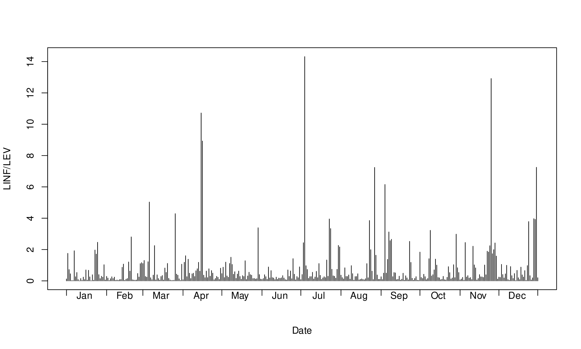
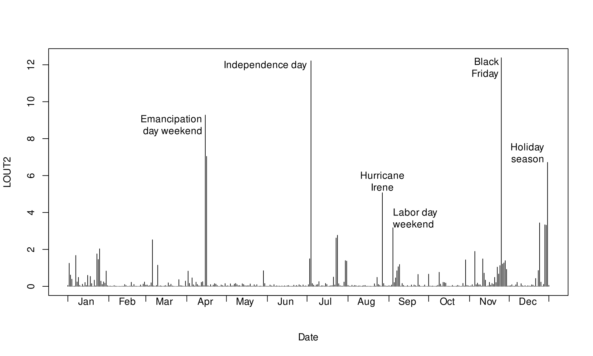
Figure 3 shows conformal local influence for each day of 2011. There are two outstandingly influential periods which are identified below. There were no days with outstandingly high leverage so a leverage plot is not shown. Figure 4 shows potential outliers based on . In addition to the highly influential days identified by figure 3, this figure highlights several other periods where the model does not fit well. A cleaner version of figure 4 can be obtained by truncating the eigenvalue expansion of the outlier matrix , as described in section 5. A scree plot (not shown) suggests that the first 7 principal components of may be sufficient to capture the most interesting variation. Figure 5 shows only the sum of the contributions to from these 7 principal components. The text labels identify the most important outliers, most of which are associated with public holidays. Interestingly, outlying days do not necessarily coincide with the public holiday but may occur the day before (e.g. the Sunday before Labor Day) or after (e.g. the Friday following Thanksgiving, popularly known as “Black Friday”). A cluster of outlying days is also visible at the end of the year, and to a lesser extent in the period around Thanksgiving. Figure 5 also highlights 27 August 2011 as an outlier. On this day, hurricane Irene hit the North Eastern United States. Anticipation of the incoming storm led to under-use of the Capital Bikeshare scheme until it was shutdown at 18:00.
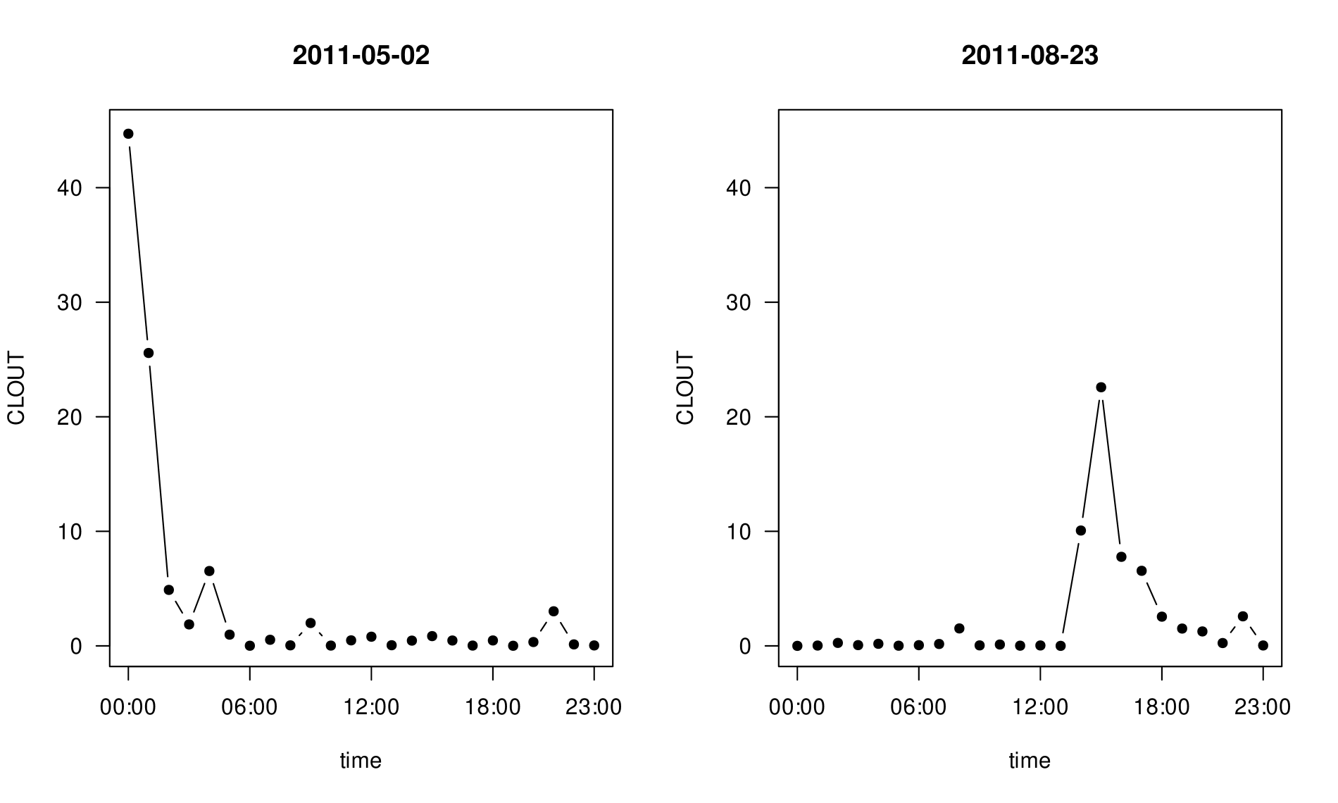
The analysis of daily influence and leverage captures important differences in user behaviour that extend across whole days, but misses more short term changes. These can be detected by analysing the data at its original hourly scale. The most outlying hour, as measured by the CLOUT statistic was from 0:00 to 1:00 on 2 May. The second most outlying hour, excluding previously identified holiday periods, was 15:00 to 16:00 on 23 August. Figure 2 shows hourly CLOUT statistics for these two days. The reason for these outliers can be readily identified from the public record. On 1 May 2011 at 23:35, President Obama announced the death of Osama Bin Laden on live television. In the following hours, there were spontaneous gatherings in the centre of Washington, leading to an increase in the number of bicycles hired in the small hours of the morning when the network is typically very quiet. On 26 August at 13:51, there was a magnitude 5.8 earthquake in the Piedmont region of Virginia. This severely disrupted transport networks in Washington DC, leading to an increase in bicycle hiring as commuters sought alternative forms of transport.

8.1 Hawkins-Bradu-Kass data
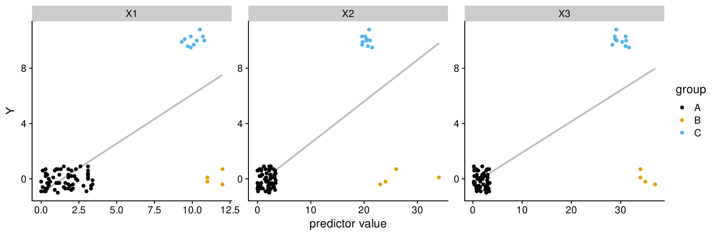
The Hawkins-Bradu-Kass (HBK) data is an artificial data set (Hawkins et al.,, 1984) that challenges outlier detection methods based on perturbing a single observation. Figure 6 illustrates the pairwise relationships between the three predictor variables and outcome in the HBK data. The observations can be clustered into 3 groups: group A, which constitutes the majority of the observations, shows no relationship between the predictor variables and the outcome; group B consists of observations that have high-leverage with respect to group A but maintain the same null relationship with ; group C are all outliers that pull the fitted least squares line away from the null.
The masking effect of multiple outliers makes the detection of the outlying group impossible using univariate methods that consider only one observation at a time. Thomas et al., (2018) show how the 3 clusters of observations can be detected after fitting a Bayesian linear model by applying multivariate analysis methods to the posterior variance matrix of the log likelihood contributions.
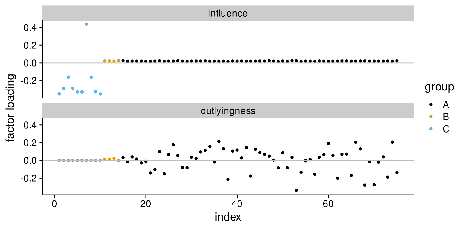
In a frequentist analysis, outlier-robust linear regression methods can be used to identify group C as a set of outliers and, after down-weighting their influence, reveal the underlying null relationship in groups A and B. In a Bayesian analysis, one way to improve robustness of a linear model is to use a 2-component normal mixture for the outcome variable . This allows a small proportion of the data to be contaminated with observations with a distinct mean and variance from the rest. Details of the mixture model are given in the supplementary materials. After fitting the mixture model, figure 7 shows the loadings for the first principal component of (top panel) and (bottom panel). The top panel shows the direction of the perturbation that is maximally influential. This perturbation puts the highest loads on observations in group C. The bottom panel shows the maximally outlying perturbation, where observations in group C are given almost zero weight. The observations in group C are collectively influential but are not considered outliers in a mixture model that explicitly accounts for the presence of anomalous observations.
9 Prior-data conflict
Gelman et al., (2004, p. 182) suggested an alternative penalty for DIC that avoids some of the known problems of discussed in section 4.1. Their penalty is based on the posterior variance of the log-likelihood.
This superficially resembles the WAIC penalty . However is based on the variance of the sum of the log-likelihood contributions from each observations, whereas is the sum of the variances. Moreover is scaled by a factor of 2 to ensure in the non-informative limit. In a retrospective review of DIC, Spiegelhalter et al., (2014) reported that they had considered as an alternative penalty to , but rejected it.
Like all of the previously considered penalty functions can be interpreted in terms of local influence. From equation (6), is local influence associated with the perturbation for small values of . The conformal local influence of this perturbation is
Informally, measures the sensitivity of the posterior to the addition of new data that are similar to the observed data. High sensitivity to this perturbation would indicate a problem with the model fit, suggesting that the ratio could be used directly as a model diagnostic.
9.1 pV in the linear model
Returning to the linear model of section 2.1, the two penalties can be written in terms of residuals and the hat matrix
| (24) | ||||
| (25) |
Equation (25) is a multivariate version of (24), with an additional calibration factor of 2. However, the two expressions behave quite differently in the non-informative limit. In this case, the first term in (24) is and the second term is . Conversely, the first term in (25) vanishes for a non-informative prior, and the second term is since is an idempotent matrix of rank in this case. Thus, although both and tend to for a non-informative prior, they do so in different ways. This suggests that they are measuring different underlying quantities.
The first term in (25) can be rewritten as
where is the information sandwich
and is the Fisher information. Hence grows when the posterior mean is far from the maximum likelihood estimate according to the metric . This distance can only be large when there is an informative prior that is pulling the posterior mean away from the maximum likelihood estimate . Hence in the linear model measures conflict between the prior and the data. It is plausible that could be used as a diagnostic for prior-data conflict in a wider class of models, especially those with a local linear representation.
9.2 Examples of prior-data conflict
Three examples below illustrate the use of as a diagnostic for prior-data conflict. Two of the examples use the binomial distribution where . There is some ambiguity in the definition of for binomial data. If is considered the smallest unit of observation, then its contribution to is
| (26) |
Conversely, if is considered as the sum of independent Bernoulli trials, each of which can be individually perturbed, then their aggregate contribution to is
| (27) |
The appropriate expression to use depends on the context. If a binomial outcome is obtained by repeated Bernoulli trials on the same observational unit then is more appropriate. Conversely, if a binomial random variable is created by aggregating Bernoulli outcomes on different observational units that share the same predictor variables then is more appropriate. These two scenarios give the same likelihood under the model, but suggest different perturbations to the data. In the examples used below, the latter penalty is used.
9.2.1 UNOS data
The first example is adapted from Gelfand, (2003) using data from the United Network for Organ Sharing (UNOS). The data concerns heart transplants that took place in 10 centres across 5 age groups. Let represent the number of adverse outomes – organ rejections or deaths – out of transplants in centre , age group . This is modelled by a mixed-effects logistic regression model
| (28) |
where is the midpoint age in group , centred and scaled so that a unit increase in represents a 10-year age difference.
The parameters are fixed effects and are centre-specific random effects for the intercept and slope.
with a sum-to-zero constraint .
Figure 8 shows the posterior distributions of the fixed effects from a reference model that uses diffuse normal priors for and weakly informative half- priors on (Full details of the model are given in the supplementary materials). The posteriors from this model are consistent with maximum likelihood estimates given by the glmer function in the R package lme4 (Bates et al.,, 2015), shown by the vertical grey lines. Figure 8 also shows alternative informative priors represented by the red dotted lines:
| (29) |
The informative priors take the prior probability mass further away from the maximum likelihood estimates. Focusing on , we consider the effect of increasing the prior-data conflict in two ways: firstly by shifting the prior mean further away from , and secondly by concentrating the prior distribution about a fixed mean. The results are shown in table 2.
| Prior on | |||||
| mean | sd | ||||
| Reference | 11.5 | 11.6 | 18.8 | 1.6 | |
| Mean shift | |||||
| -0.9 | 0.20 | 10.7 | 10.6 | 19.4 | 1.8 |
| -0.7 | 0.20 | 10.4 | 10.2 | 20.3 | 2.0 |
| -0.5 | 0.20 | 10.1 | 9.8 | 21.8 | 2.2 |
| -0.3 | 0.20 | 10.0 | 9.6 | 23.4 | 2.4 |
| -0.1 | 0.20 | 9.8 | 9.3 | 26.2 | 2.8 |
| Concentration | |||||
| -0.9 | 0.20 | 10.6 | 10.5 | 19.4 | 1.8 |
| -0.9 | 0.10 | 9.8 | 9.4 | 21.2 | 2.3 |
| -0.9 | 0.05 | 8.6 | 8.0 | 20.7 | 2.6 |
| -0.9 | 0.02 | 7.7 | 7.0 | 15.9 | 2.3 |
| -0.9 | 0.01 | 7.6 | 6.9 | 13.9 | 2.0 |
The first row of table 2 shows the results for the reference model. The ratio may seem surprisingly high for model with a weakly informative prior. Note however that we only expect asymptotically for large . In this example there are binomial observations with an effective number of parameters so the sample size may not be large enough for this asymptotic result to hold.
Row 2 of table 2 shows results for the informative prior (29) which shows a modest increase in to 1.8. Rows 3-6 show the effect of shifting the prior mean further away from . Each shift, equal to 1 prior standard deviation, leads to a further increase in .
Rows 7-11 of table 2 show the effect of fixing the prior mean at but reducing the prior standard deviation by approximately half each time. The ratio is not a monotonic function of the concentration. It reaches a maximum of 2.6 for a prior standard deviation sd=0.05, then decreases to 2.3 for sd=0.02 and 2.0 for sd=0.01. This phenomenon may be explained by the fact that a sufficiently strong prior resolves prior-data conflict in favour of the prior, so that the posterior becomes insensitive to perturbations to the data.
9.2.2 Bristol Royal Infirmary inquiry data
In addition to detecting global prior-data conflict, the ratio may be used to investigate divergent behaviour at different levels of a hierarchical model. This is illustrated with data from the Bristol Royal Infirmary inquiry presented by Marshall and Spiegelhalter, (2007). The inquiry investigated claims of excess mortality in paediatric cardiac surgery carried out at the Bristol Royal Infirmary prior to 1995 (Spiegelhalter et al., 2002a, ). Panel A of figure 9 shows mortality in 12 hospitals where comparable cardiac surgeries took place.
Let be the number of deaths among operations carried out at hospital . Then the data can be analysed using a random effects model
| (30) |
with uniform priors on the hyper-parameters .
Taking a cross-validation approach, let be the data for all hospitals except hospital . If the focus of interest is on hospital then we can consider as the likelihood and as a prior distribution for that subsumes all information from the other hospitals. Then there are 12 sets of paired statistics , one for each hospital, where is defined by perturbing each of the operations individually as in equation (27) and is defined by a single common perturbation to all operations in hospital as in equation (26).
Rather than measuring prior-data conflict, the ratio measures cross-conflict between different hospitals, since the cross-validation prior incorporates information from all other hospitals. Note that the ratio does not require an explicit calculation of of the cross-validation prior, nor does it require that be expressed in closed form.
The results are shown in panel B of figure 9. As might be expected from the context, the Bristol Royal Infirmary shows the largest cross-conflict with . This is roughly double the cross-conflict for Leeds , where mortality was lower than average (Panel A). The remaining hospitals show cross-conflict values close to 1.

9.2.3 HBK data
The artificial HBK data from section 8.1 illustrates extreme cross-conflict. If any one of the observation groups A,B, or C is removed, then the omitted data will be in contradiction with a linear regression line fitted to the remaining two groups (See Figure 6). To quantify this, the cross-conflict ratio was calculated for each group in turn. The results are shown in table 3. The top row shows the results for a linear model with a normal error distribution. This shows very high cross-conflict ratios for all groups with group A having the highest ratio with . The second row shows results for the mixture model fitted in section 8.1. Cross-conflict ratios are substantially reduced compared to the linear model but still high for groups A (4.4) and C (7.9). The use of an outlier-robust mixture model does not eliminate the cross-conflict, which is a feature of the data, not the model.
| Model | Group | ||
|---|---|---|---|
| A | B | C | |
| Normal | 59.5 | 4.89 | 17.6 |
| Normal mixture | 4.4 | 1.81 | 7.9 |
10 Discussion
Bayesian sensitivity analysis has often concentrated on prior sensitivity (Roos et al.,, 2015) since the presence of a prior distribution distinguishes Bayesian from frequentist inference. Bayesian and frequentist models share a common problem that they may be sensitive to changes in the data. The sensitivity diagnostics discussed here do not test any specific deviation from the working model, and hence may point to a variety of different issues, including: errors in the data, failure to capture certain data features in the working model, and conflict between the data and an informative prior.
The project management triangle is a theory that competing constraints of cost, scope, and time cannot be simultaneously satisfied. It is often expressed as “Good, fast, cheap. Choose two.” The diagnostics discussed here are fast, since they can be derived from the same MCMC run used to estimate the model parameters. They are cheap, since they involve monitoring quantities that are easy to calculate. The question arises of whether they are good. I hope that the examples show they can be useful. However, there is no guarantee that these diagnostics will work across the entire spectrum of Bayesian modelling. I do not suggest that they can replace more formal diagnostics when the investigator suspects the risk of a particular departure from the model assumptions. Moreover, when they reveal previously unsuspected problems, this should be the start of a more comprehensive diagnostic work-up.
One issue with the conformal diagnostics CLINF, CLLEV and CLOUT is that they are not calibrated. There is no rule that gives a cut-off for anomalous observations. This is a problem that is shared with frequentist measures of leverage and influence. Although some heuristic rules have been suggested for frequentist diagnostics, my view is that the answer will depend on the context and we can only distinguish observations that have relatively high leverage, influence, or outlyingness compared with the others. Some kind of threshold is however required for the use of as a diagnostic for prior-data conflict since this analysis produces only a single number. Based on the limited exploration in section 9, I would tentatively suggest that could be used as a threshold for further investigation.
There is a strong connection between local influence and predictive information criteria. All information criteria are based on the same principle that aims to correct for optimism in a numeric assessment of model fit by adding a complexity penalty. Over-fitted models are likely to be both highly optimistic – hence requiring a large penalty – and be sensitive to small changes to the data. So intuitively it is not surprising to find this connection. It is interesting that the penalties used by WAIC and DIC can be derived in a rigorous way from the same local sensitivity framework based on phi-divergences. This connection may also help to understand the differences between WAIC and DIC. The WAIC penalty penalizes an aggregate measure of influence whereas the alternative DIC penalty penalizes an aggregate measure of leverage. The Bayesian concept of leverage is derived from a posterior predictive framework and is closely related to Value of Information analysis, in which decisions are guided by the assumption that the model is true. Hence the main difference between WAIC and DIC is that the latter incorporates an explicit “good model” assumption.
The alternative DIC penalty measures sensitivity to a particular perturbation of the data that may reveal prior-data conflict. Whereas and are often numerically very similar, section 9 shows that may penalize models much more strongly in the presence of prior-data conflict. This phenomenon might actually make a more attractive penalty for model choice since ceteris paribus we would normally want to choose a model without prior-data conflict. However, currently only has a heuristic justification in the model choice context. The ratio may be re-purposed to diagnose cross-conflict between different parts of the data. This may have interesting applications in modular inference, where the presence of cross-conflict is the justification for departing from the standard rules of Bayesian updating (Jacob et al.,, 2017; Carmona and Nicholls,, 2020).
Appendix A Supplementary Material
R and JAGS code for all examples is available at
The examples require JAGS 5.0.0 or later.
References
- Akaike, (1973) Akaike, H. (1973). Information theory and an extension of the maximum likelihood principle. Proceedings of the Second International Symposium on Information Theory, pages 267–281.
- Bates et al., (2015) Bates, D., Mächler, M., Bolker, B., and Walker, S. (2015). Fitting linear mixed-effects models using lme4. Journal of Statistical Software, 67(1):1–48.
- Beckman et al., (1987) Beckman, R. J., Nachtsheim, C. J., and Cook, R. D. (1987). Diagnostics for mixed-model analysis of variance. Technometrics, 29(4):413.
- Brooks et al., (2002) Brooks, S. P., Smith, J., Vehtari, A., Plummer, M., Stone, M., Robert, C. P., Titterington, D. M., Nelder, J. A., Atkinson, A., Dawid, A. P., et al. (2002). Discussion on the paper by spiegelhalter, best, carlin and van der linde. Journal of the Royal Statistical Society: Series B (Statistical Methodology), 64(4):616–639.
- Carmona and Nicholls, (2020) Carmona, C. and Nicholls, G. (2020). Semi-modular inference: enhanced learning in multi-modular models by tempering the influence of components. In Chiappa, S. and Calandra, R., editors, Proceedings of the Twenty Third International Conference on Artificial Intelligence and Statistics, volume 108 of Proceedings of Machine Learning Research, pages 4226–4235. PMLR.
- Christensen et al., (1992) Christensen, R., Pearson, L. M., and Johnson, W. (1992). Case-deletion diagnostics for mixed models. Technometrics, 34(1):38–45.
- Cook, (1986) Cook, R. D. (1986). Assessment of local influence. Journal of the Royal Statistical Society. Series B, Methodological, 48(2):133–169.
- Cook and Weisberg, (1982) Cook, R. D. and Weisberg, S. (1982). Residuals and influence in regression. Chapman and Hall, London;New York;.
- Demidenko and Stukel, (2005) Demidenko, E. and Stukel, T. A. (2005). Influence analysis for linear mixed-effects models. Statistics in medicine, 24(6):893–909.
- Drton and Plummer, (2017) Drton, M. and Plummer, M. (2017). A Bayesian information criterion for singular models. Journal of the Royal Statistical Society. Series B, Statistical methodology, 79(2):323–380.
- Fanaee-T, (2013) Fanaee-T, H. (2013). Bike Sharing. UCI Machine Learning Repository.
- Gelfand, (2003) Gelfand, A. E. (2003). Some comments on model criticism. In Green, P. J., Hjort, N. L., and Richardson, S., editors, Highly Structured Stochastic Systems, pages 449–454. Oxford University Press, Oxford, UK.
- Gelman et al., (2004) Gelman, A., Carlin, J. B., and Stern, Hal S. Rubin, D. B. (2004). Bayesian Data Analysis. Chapman and Hall/CRC, 2 edition.
- Gelman et al., (2014) Gelman, A., Hwang, J., and Vehtari, A. (2014). Understanding predictive information criteria for bayesian models. Statistics and computing, 24(6):997–1016.
- Hastie and Tibshirani, (1990) Hastie, T. and Tibshirani, R. (1990). Generalized additive models, volume 43. Chapman and Hall, London.
- Hawkins et al., (1984) Hawkins, D. M., Bradu, D., and Kass, G. V. (1984). Location of several outliers in multiple-regression data using elemental sets. Technometrics, 26(3):197–208.
- Hodges and Sargent, (2001) Hodges, J. S. and Sargent, D. J. (2001). Counting degrees of freedom in hierarchical and other richly‐parameterised models. Biometrika, 88(2):367–379.
- Jackson et al., (2022) Jackson, C. H., Baio, G., Heath, A., Strong, M., Welton, N. J., and Wilson, E. C. F. (2022). Value of information analysis in models to inform health policy. Annual review of statistics and its application, 9(1):95–118.
- Jacob et al., (2017) Jacob, P., Murray, L., Holmes, C., and Robert, C. (2017). Better together? statistical learning in models made of modules. arXiv.
- Kelly et al., (2023) Kelly, M., Longjohn, R., and Nottingham, K. (2023). The UCI machine learning repository. Accessed: 2024-02-18.
- Lavine, (1992) Lavine, M. (1992). Local predictive influence in Bayesian linear models with conjugate priors. Communications in statistics. Simulation and computation, 21(1):269–283.
- Lesaffre and Verbeke, (1998) Lesaffre, E. and Verbeke, G. (1998). Local influence in linear mixed models. Biometrics, 54(2):570–582.
- Marshall and Spiegelhalter, (2007) Marshall, E. C. and Spiegelhalter, D. J. (2007). Identifying outliers in Bayesian hierarchical models: a simulation-based approach. Bayesian analysis, 2(2).
- McCulloch, (1989) McCulloch, R. E. (1989). Local model influence. Journal of the American Statistical Association, 84(406):473–478.
- Millar, (2018) Millar, R. B. (2018). Conditional vs marginal estimation of the predictive loss of hierarchical models using waic and cross-validation. STATISTICS AND COMPUTING, 28(2):375–385.
- Millar and Stewart, (2007) Millar, R. B. and Stewart, W. S. (2007). Assessment of locally influential observations in Bayesian models. Bayesian Analysis, 2(2):365 – 383.
- (27) Nash, W., Sellers, T., Talbot, S., Cawthorn, A., and Ford, W. (1994a). Abalone. UCI Machine Learning Repository.
- (28) Nash, W., Sellers, T., Talbot, S., Cawthorn, A., and Ford, W. (1994b). The population biology of abalone (haliotis species) in tasmania. i. blacklip abalone (h. rubra) from the north coast and islands of bass strait. Technical Report 48, Sea Fisheries Division.
- Nelder and Wedderburn, (1972) Nelder, J. A. and Wedderburn, R. W. M. (1972). Generalized linear models. Journal of the Royal Statistical Society. Series A (General), 135(3):370–384.
- Nobre and Singer, (2011) Nobre, J. S. and Singer, J. M. (2011). Leverage analysis for linear mixed models. Journal of applied statistics, 38(5):1063–1072.
- Ouwens et al., (2001) Ouwens, M. J. N. M., Tan, F. E. S., and Berger, M. P. F. (2001). Local influence to detect influential data structures for generalized linear mixed models. Biometrics, 57(4):1166–1172.
- Parsons and Bao, (2022) Parsons, J. and Bao, L. (2022). A unified approach for outliers and influential data detection: The value of information in retrospect. Stat (International Statistical Institute), 11(1):e442.
- Plummer, (2002) Plummer, M. (2002). Discussion on the paper by spiegelhalter, best, carlin and van der linde. Journal of the Royal Statistical Society: Series B (Statistical Methodology), 64(4):620 –621.
- Plummer, (2008) Plummer, M. (2008). Penalized loss functions for bayesian model comparison. Biostatistics, 9(3):523–539.
- Poon and Poon, (1999) Poon, W.-Y. and Poon, Y. S. (1999). Conformal normal curvature and assessment of local influence. Journal of the Royal Statistical Society. Series B, Statistical methodology, 61(1):51–61.
- Rakhmawati et al., (2017) Rakhmawati, T. W., Molenberghs, G., Verbeke, G., and Faes, C. (2017). Local influence diagnostics for generalized linear mixed models with overdispersion. Journal of Applied Statistics, 44(4):620–641.
- Roos et al., (2015) Roos, M., Martins, T. G., Held, L., and Rue, H. (2015). Sensitivity analysis for bayesian hierarchical models. Bayesian analysis, 10(2).
- Ryan et al., (2016) Ryan, E. G., Drovandi, C. C., McGree, J. M., and Pettitt, A. N. (2016). A review of modern computational algorithms for bayesian optimal design. International Statistical Review / Revue Internationale de Statistique, 84(1):128–154.
- (39) Spiegelhalter, D. J., Aylin, P., Best, N. G., Evans, S. J. W., and Murray, G. D. (2002a). Commissioned analysis of surgical performance using routine data: lessons from the bristol inquiry. Journal of the Royal Statistical Society. Series A, Statistics in society, 165(2):191–221.
- (40) Spiegelhalter, D. J., Best, N. G., Carlin, B. P., and van der Linde, A. (2002b). Bayesian measures of model complexity and fit. Journal of the Royal Statistical Society: Series B (Statistical Methodology), 64(4):583–639.
- Spiegelhalter et al., (2014) Spiegelhalter, D. J., Best, N. G., Carlin, B. P., and van der Linde, A. (2014). The deviance information criterion: 12 years on. Journal of the Royal Statistical Society: Series B (Statistical Methodology), 76(3):485–493.
- Thomas et al., (2018) Thomas, Z. M., MacEachern, S. N., and Peruggia, M. (2018). Reconciling curvature and importance sampling based procedures for summarizing case influence in bayesian models. Journal of the American Statistical Association, 113(524):1669–1683.
- van der Linde, (2007) van der Linde, A. (2007). Local influence on posterior distributions under multiplicative modes of perturbation. Bayesian Analysis, 2(2):319 – 332.
- Wahba, (1990) Wahba, G. (1990). Spline models for observational data, volume 59. Society for Industrial and Applied Mathematics, Philadelphia, Pa.
- Watanabe, (2009) Watanabe, S. (2009). Algebraic Geometry and Statistical Learning Theory. Cambridge University Press.
- Watanabe, (2010) Watanabe, S. (2010). Asymptotic equivalence of bayes cross validation and widely applicable information criterion in singular learning theory. Journal of Machine Learning Research, 11(116):3571–3594.
- Waugh, (1995) Waugh, S. (1995). Extending and benchmarking Cascade-Correlation : extensions to the Cascade-Correlation architecture and benchmarking of feed-forward supervised artificial neural networks. PhD thesis, University of Tasmania.
- Zhu and Lee, (2001) Zhu, H.-T. and Lee, S.-Y. (2001). Local influence for incomplete data models. Journal of the Royal Statistical Society. Series B, Statistical methodology, 63(1):111–126.