Weak Convergence Analysis for the Finite Element Approximation to Stochastic Allen-Cahn Equation Driven by Multiplicative White Noise

Abstract

In this paper, we aim to study the optimal weak convergence order for the finite element approximation to a stochastic Allen-Cahn equation driven by multiplicative white noise. We first construct an auxiliary equation based on the splitting-up technique and derive prior estimates for the corresponding Kolmogorov equation and obtain the strong convergence order of 1 in time between the auxiliary and exact solutions. Then, we prove the optimal weak convergence order of the finite element approximation to the stochastic Allen-Cahn equation by deriving the weak convergence order between the finite element approximation and the auxiliary solution via the theory of Kolmogorov equation and Malliavin calculus. Finally, we present a numerical experiment to illustrate the theoretical analysis.

MSC Classification]60H15, 60H35, 65C30

1 Introduction

Over the past decades, numerical analysis of stochastic partial differential equations (SPDEs) has attracted increasing attention [1, 2, 3, 4, 5, 6, 7]. Both strong and weak convergence rates of the numerical approximation for SPDEs under globally Lipschitz continuity condition have been widely studied [8, 9, 10, 11, 12]. However, many practical models, such as the stochastic Allen-Cahn equation to be discussed in this work, fail to satisfy such a condition, which motivates studies on SPDEs with non-globally Lipschitz coefficient [13, 14, 15, 16].

The stochastic Allen-Cahn equation models the effect of thermal perturbations, and plays an important role in phase-field theory and the simulations of rare events in infinite dimensional stochastic systems [17]. Numerical approximations for the stochastic Allen-Cahn equations have been studied extensively in the last decade. Initial studies focused on the strong convergence of numerical approximation to the stochastic Allen-Cahn equation driven by additive noise. Kovács et al. [18, 19] studied the strong convergence order for a temporal semi-discretization with an implicit Euler method. Bréhier et al. [20, 21] introduced an explicit time discretization scheme based on a splitting strategy and analyzed its strong convergence order. Qi and Wang [22] analyzed the optimal strong convergence order of a full discretization using the FEM and the implicit Euler method. Wang [23] applied a spectral Galerkin method and a tamed accelerated exponential Euler method to set up a full discretization and proved the strong convergence order. Recently, the stochastic Allen-Cahn equation driven by multiplicative noise has also been studied. Liu and Qiao [24] constructed a drift-implicit Euler-Galerkin scheme and derived the optimal strong convergence order. Huang and Shen [25] applied the spectral Galerkin method and tamed semi-implicit Euler method to set up a fully discretized approximation, and analyze its strong convergence order as well as unconditional stability. Yang et al. [26] discretized stochastic Allen-Cahn equation by the implicit Euler scheme in time and the discontinuous Galerkin method in space and obtained its optimal strong convergence rate.

In this paper, we are concerned with the weak convergence of numerical approximations of the stochastic Allen Cahn equation driven by multiplicative noise. The weak error, sometimes more relevant in various fields such as finance and engineering, concerns with the approximation of the probability distribution of solutions to SPDEs [27, 28]. It measures the error made by sampling from an approximate probability law of the exact solution, rather than the deviation from trajectory of the exact solution, as for the strong error [8, 29]. In recent years, several stratgies have been proposed to analyze weak errors of numerical approximation to SPDEs with Lipschitz continuous coefficients. These stratgies include Kolmogorov equation method [8, 30, 31, 32], the mild Itô formula [33, 34] and others [35, 36]. Cui et al.  constructed a full discretization scheme by FEM and backward Euler method, and obtained the optimal weak convergence order for spatial semi-discretization [37] and for full discretization [38]. Cai et al. [39] discretized the stochastic Allen-Cahn equation driven by an additive noise using a spectral Galerkin method and a tamed exponential Euler method and then investigated the weak convergence order.

To the best of our knowledge, there has been no prior work on weak error estimates for the finite element method (FEM) applied to the stochastic Allen-Cahn equation driven by multiplicative noise. Addressing this gap is the primary focus of this work. The main analytical challenge lies in deriving high-order, uniform a priori estimates for the Fréchet derivatives of the solution to the associated Kolmogorov equation. In case where the nonlinear forcing term of a SPDE satisfies a uniform Lipschitz condition [8], the Fréchet derivatives of Kolmogorov equation with respect to initial value under the action of a fractional power of the Laplacian operator satisfies an SPDE with uniform bounded coefficient functions, which can be easily dealt with. For the Allen-Cahn equation driven by an additive noise [37], the counterpart satisfies a PDE without a noise forcing term. In this case, The techniques for deterministic PDE can be applied to obtain uniform estimates for the Fréchet derivatives under the action of a fractional power of the Laplacian operator, and these estimates directly yield the weak convergence order.

The Allen-Cahn equation driven by multiplicative noise introduces additional challenges in analyzing prior estimates for the solution of the Kolmogorov equation. Specifically, the Fréchet derivatives of the Kolmogorov equation’s solution with respect to the initial value satisfy an SPDE driven by multiplicative noise, characterized by a one-sided Lipschitz coefficient function. A key innovation of our work is the application of the mild Itô formula [40] to the Kolmogorov equation. This approach enables us to establish the uniform boundedness of the first- and second-order Fréchet derivatives. Furthermore, to achieve the desired weak convergence order, we introduce a novel method that transfers the action of the fractional power of the Laplacian operator from the Kolmogorov equation’s solution to the mild solution of the FEM approximation. This technique allows us to rigorously prove the weak convergence order for the stochastic FEM approximation.

Our strategy for obtaining the optimal weak convergence order consists of two main steps:

1. Temporal Splitting and Auxiliary SPDE: We construct a temporal splitting approximation for the stochastic Allen-Cahn equation and define an auxiliary SPDE. We establish a strong convergence order of 1 in time between the exact solution and the auxiliary solution and derive the regularity estimates for the corresponding Kolmogorov equation.

2. Weak Convergence Analysis: Using Malliavin calculus and the Kolmogorov equation, we analyze the weak convergence order between the FEM approximation and the auxiliary solution. The optimal weak convergence order between the FEM approximation and the exact solution follows as a direct result.

We note that while we achieve a first-order convergence rate in the weak sense, only a half-order convergence rate is attainable in the strong sense ([23, 39]).

The rest of this paper is organized as follows. In section 2, we introduce some preliminaries and main assumptions, and give a brief introduction to Malliavin calculus. In section 3, we construct an auxiliary equation based on splitting-up technique, and investigate the strong convergence order in time between the exact and auxiliary solutions. In section 4, we construct an FEM semi-discretization, and present a regularity estimate of its Malliavin derivative. In section 5, we analyze the weak convergence order of the finite element semi-discretization to the auxiliary equation. In section 6, we carry out a numerical experiment to demonstrate the theoretical analysis.

2 Preliminaries

2.1 Some spaces and properties

Let $(U,(\cdot,\cdot)_{U})$ and $(V,(\cdot,\cdot)_{V})$ be two real separable Hilbert spaces and $(\Omega,\mathcal{F},\mathbb{P})$ be a complete probability space. By $\mathcal{L}(U,V)$ we denote the Banach space of all bounded linear operators from $U$ to $V$ endowed with operator norm. For simplicity, we write $\mathcal{L}(U)=\mathcal{L}(U,U)$. If $T\in\mathcal{L}(U)$, then $\|T\|_{\mathcal{L}(U)}=\|T^{*}\|_{\mathcal{L}(U)}$.

For any $T\in\mathcal{L}(U)$, let $\{\sigma_{k}\}_{k\in\mathbb{N}}$ be eigenvalues of $(TT^{*})^{\frac{1}{2}}$. For any $1\leq p<\infty$, define a Banach space of linear operators

$$\mathcal{L}_{p}(U)=\big{\{}T\in\mathcal{L}(U):\ \|T\|_{\mathcal{L}_{p}(U)}=\big{(}\sum_{k=1}^{\infty}\sigma_{k}^{p}\big{)}^{\frac{1}{p}}<\infty\big{\}}.$$

Let $\{e_{k}\}_{k=1}^{\infty}$ be an orthonormal basis of $U$. Define $\mathrm{Tr}(T)=\sum_{k=1}^{\infty}(Te_{k},e_{k})_{U}$ if the summation is finite. Obviously, $\mathcal{L}_{1}(U)$ is the space of trace class operators. For any $T\in\mathcal{L}_{1}(U)$, we have $|\mathrm{Tr}(T)|\leq\|T\|_{\mathcal{L}_{1}(U)}$ and the equality holds if $T$ is positive semidefinite. Furthermore, for any $S\in\mathcal{L}(U)$, there hold [41, 9]

$$\mathrm{Tr}(T)=\mathrm{Tr}(T^{*}),\ \mathrm{Tr}(TS)=\mathrm{Tr}(ST),$$ (1)

$$\mathrm{Tr}(ST)\leq\|ST\|_{\mathcal{L}_{1}(U)}\leq\|S\|_{\mathcal{L}(U)}\|T\|_{\mathcal{L}_{1}(U)},$$

$$\mathrm{Tr}(TS)\leq\|TS\|_{\mathcal{L}_{1}(U)}\leq\|S\|_{\mathcal{L}(U)}\|T\|_{\mathcal{L}_{1}(U)}.$$

By $\mathcal{L}_{2}(U,V)$ we denote the space of Hilbert-Schmidt operators from $U$ to $V$, which is also a Hilbert space with inner product and norm

$$(S,T)_{\mathcal{L}_{2}(U,V)}=\sum_{k=1}^{\infty}(Se_{k},Te_{k})_{V}=\mathrm{Tr}(T^{*}S),\ \|T\|^{2}_{\mathcal{L}_{2}(U,V)}=\mathrm{Tr}(TT^{*}).$$ (2)

For simplifying notations, we denote by $\mathcal{L}_{2}(U)=\mathcal{L}_{2}(U,U)$. Then for any $S\in\mathcal{L}(U)$, $T_{1},T_{2}\in\mathcal{L}_{2}(U)$, there hold that [41, 9]

$$\|T_{1}\|_{\mathcal{L}(U)}\leq\|T_{1}\|_{\mathcal{L}_{2}(U)},$$ (3)

$$\|ST_{1}\|_{\mathcal{L}_{2}(U)}\leq\|S\|_{\mathcal{L}(U)}\|T_{1}\|_{\mathcal{L}_{2}(U)},$$

$$\|T_{1}S\|_{\mathcal{L}_{2}(U)}\leq\|S\|_{\mathcal{L}(U)}\|T_{1}\|_{\mathcal{L}_{2}(U)},$$

$$\|T_{1}T_{2}\|_{\mathcal{L}_{1}(U)}\leq\|T_{1}\|_{\mathcal{L}_{2}(U)}\|T_{2}\|_{\mathcal{L}_{2}(U)}.$$

For any integer $m\geq 1$, by $\mathcal{C}_{b}^{m}(U)$ we denote the space of not necessarily bounded functions $\phi:U\rightarrow\mathbb{R}$ having $m$-th continuous and bounded Fréchet derivatives $D\phi,D^{2}\phi,\cdots,D^{m}\phi$. We endow it with the seminorm $|\cdot|_{\mathcal{C}_{b}^{m}(U)}$, defined as the smallest constant $C\geq 0$ satisfying

$$\sup_{u\in U}|D^{m}\phi(u)(h_{1},\cdots,h_{m})|\leq C\|h_{1}\|_{U}\cdots\|h_{m}\|_{U},\quad\forall h_{1},\cdots,h_{m}\in U.$$

Let $D\phi(u)$ denote the first order Fréchet derivative of $\phi$ at $u\in U$, which is a bounded linear functional on $U$. According to Riesz representation theorem, there exists a unique element in $U$, still denoted by $D\phi(u)$, such that for any $h\in U$

$$D\phi(u)h=(D\phi(u),h)_{U},\quad|D\phi(u)h|\leq|\phi|_{\mathcal{C}_{b}^{1}(U)}\|h\|_{U}.$$ (4)

2.2 Stochastic Allen-Cahn equation and assumptions

In this section, we first describe the stochastic Allen-Cahn equation driven by multiplicative white noise and assumptions, and then collect some properties of its solution.

Let $L$ be a positive number and define $\mathcal{D}=(0,L)$. By $H=L^{2}(\mathcal{D})$ we denote the standard Sobolev space with inner product $(\cdot,\cdot)$ and norm $\|\cdot\|$. Let $V=\mathcal{C}(\bar{\mathcal{D}})$ be the space of continuous functions endowed with maximum norm $\|\cdot\|_{V}$.

Consider a semilinear parabolic SPDE with homogeneous Dirichlet boundary condition driven by multiplicative white noise

$$dX(t,x)-\Delta X(t,x)dt= \ F(X(t,x))dt+G(X(t,x))dW(t),\ t\in(0,T],x\in\mathcal{D},$$ (5)

$$X(t,x)= \ 0,\ t\in(0,T],x\in\partial\mathcal{D},$$

$$\quad X(0,x)= \ \xi(x),\ x\in\mathcal{D},$$

where $T>0$ is fixed. By $X(t,x,\xi)$ we denote the mild solution of (5) satisfying $X(0,x,\xi)=\xi(x)$. For simplifying notations, we abbreviate it to $X(t,\xi)$.

Denote by $A=-\Delta:\mathrm{Dom}(A)\subset H\to H$ the Laplacian operator under homogeneous Dirichlet boundary condition, where $\operatorname{Dom}(A)=H_{0}^{1}(\mathcal{D})\cap H^{2}(\mathcal{D})$. Then, the operator $A$ possesses a family of eigenvalues $\lambda_{i}=\pi^{2}i^{2}$ with complete orthonormal eigenbases $\varphi_{i}(x)=\sqrt{2}\sin(i\pi x)\in H$. For any $\alpha\in\mathbb{R}$, we define the fractional powers of $A$ by

$$A^{\alpha}v=\sum_{i=1}^{\infty}\lambda_{i}^{\alpha}(v,\varphi_{i})\varphi_{i}.$$

Let $\dot{H}^{\alpha}=\{v\in H:\|v\|_{\alpha}=\|A^{\frac{\alpha}{2}}v\|=\big{(}\sum_{i=1}^{\infty}\lambda_{i}^{\alpha}(v,\varphi_{i})^{2}\big{)}^{\frac{1}{2}}<\infty\}$. Then $(\dot{H}^{\alpha},\|\cdot\|_{\alpha})$ is a Hilbert space. Especially, we have $\dot{H}^{0}=H$, $\dot{H}^{1}(\mathcal{D})=H_{0}^{1}(\mathcal{D})$ and $\dot{H}^{2}(\mathcal{D})=H_{0}^{1}(\mathcal{D})\cap H^{2}(\mathcal{D})$, cf. [42]. For any $\beta>\frac{1}{4}$, direct computation leads to

$$\|A^{-\beta}\|^{2}_{\mathcal{L}_{2}(H)}=\sum_{j=1}^{\infty}\|(\pi^{2}j^{2})^{-\beta}\varphi_{j}\|^{2}\leq\sum_{j=1}^{\infty}j^{-4\beta}<\infty,$$ (6)

which implies $A^{-\beta}$ is a Hilbert-Schmidt operator.

The operator $A$ generates an analytic semigroup $S(t)=e^{tA}$ on $H$. According to [42], for any $\alpha\geq 0$, there hold

$$A^{\alpha}S(t)=S(t)A^{\alpha}\ \text{ on }\dot{H}^{2\alpha}\text{ and }\|A^{\alpha}S(t)\|_{\mathcal{L}(H)}\leq Ct^{-\alpha},\quad t>0.$$ (7)

where $C=C(\alpha)>0$ is a constant.

Now we introduce assumptions used in this article.

• $F:L^{6}(\mathcal{D})\rightarrow H$ is a Nemytskii operator defined by

  $$F(u)(x)=f(u(x))=u(x)-u^{3}(x),\ \forall x\in\mathcal{D},u\in L^{6}(\mathcal{D})$$

According to [39], there hold estimates

$$\|F(u)\|_{1}\leq C_{F}(1+\|u\|_{V}^{2})\|u\|_{1},\quad\forall u\in\dot{H}^{1},$$ (8)

$$\|F(u)-F(v)\|\leq C_{F}(1+\|u\|_{V}^{2}+\|v\|_{V}^{2})\|u-v\|,\quad\forall u,v\in V,$$

$$(DF(u)v,v)\leq C_{F}\|v\|^{2},\quad\forall u,v\in L^{6}(\mathcal{D}),$$

$$\|DF(u)v\|\leq C_{F}(1+\|u\|_{V}^{2})\|v\|,\quad\forall u\in V,v\in L^{6}(\mathcal{D}),$$

$$\|D^{2}F(u)(v,w)\|\leq C_{F}\|u\|_{V}\|v\|\|w\|,\quad\forall u\in V,v,w\in L^{6}(\mathcal{D}),$$

where $C_{F}>0$ is a constant.

• $G(u)=B_{0}+B_{1}u+g(u)$, where $B_{0}\in\mathcal{L}(H)$, $B_{1}\in\mathcal{L}(\dot{H}^{-\frac{1}{2}-\delta},\mathcal{L}(H))$, $g(0)=0$ and $g\in\mathcal{C}_{b}^{2}(\dot{H}^{-\frac{1}{2}-\delta},\mathcal{L}(H))$ for a small $\delta>0$.

Remark 1.

The requirement $g(0)=0$ is natural, otherwise we can simultaneously replace $B_{0}$ and $g(u)$ by $B_{0}+g(0)$ and $g(u)-g(0)$, respectively.

The following lemma collects some properties about $G$.

Lemma 1.

For any $u\in\dot{H}^{-\frac{1}{2}-\delta}$ and $v,w\in H$, there exists a constant $C>0$, such that

$$\|G(u)\|_{\mathcal{L}(H)}\leq C(1+\|u\|_{-\frac{1}{2}-\delta}),$$

$$\|DG(u)v\|_{\mathcal{L}_{2}(H)}\leq C\|v\|,$$

$$\|D^{2}G(u)(v,w)\|_{\mathcal{L}_{2}(H)}\leq C\|v\|\|w\|.$$

Moreover, for any $u\in\dot{H}^{1}$, there exists a constant $C>0$, such that

$$\|A^{\frac{1}{2}}G(u)\|_{\mathcal{L}_{2}(H)}\leq C\|u\|_{1}.$$

Proof.

According to (A2), for any $u\in\dot{H}^{-\frac{1}{2}-\delta}$, there exists a constant $C_{G}>0$, such that $\|B_{0}\|_{\mathcal{L}(H)}\leq C_{G}$, $\|B_{1}u\|_{\mathcal{L}(H)}\leq C_{G}\|u\|_{-\frac{1}{2}-\delta}$, $\|Dg(u)\|_{\mathcal{L}(\dot{H}^{-\frac{1}{2}-\delta},\mathcal{L}(H))}\leq C_{G}$ and

$$\|g(u)\|_{\mathcal{L}(H)}=\|g(u)-g(0)\|_{\mathcal{L}(H)}=\|\int_{0}^{1}Dg(\theta u)ud\theta\|_{\mathcal{L}(H)}\leq C_{G}\|u\|_{-\frac{1}{2}-\delta}$$

Thus we have

$$\ \|G(u)\|_{\mathcal{L}(H)}\leq\|B_{0}\|_{\mathcal{L}(H)}+\|B_{1}u\|_{\mathcal{L}(H)}+\|g(u)\|_{\mathcal{L}(H)}\leq C(1+\|u\|_{-\frac{1}{2}-\delta}).$$

Furthermore, if $u\in H$ and noticing $H\hookrightarrow\dot{H}^{-\frac{1}{2}-\delta}$, there holds

$$\|G(u)\|_{\mathcal{L}(H)}\leq C_{G}(1+\|u\|_{-\frac{1}{2}-\delta})\leq C(1+\|u\|).$$ (9)

Noticing that $A^{\frac{1}{4}+\frac{1}{2}\delta}\in\mathcal{L}(H,\dot{H}^{-\frac{1}{2}-\delta})$, then we have

$$\|B_{1}A^{\frac{1}{4}+\frac{1}{2}\delta}\|_{\mathcal{L}(H,\mathcal{L}(H))}= \ \sup_{u\in H}\frac{\|B_{1}A^{\frac{1}{4}+\frac{1}{2}\delta}u\|_{\mathcal{L}(H)}}{\|u\|}$$

$$= \ \sup_{v\in\dot{H}^{-\frac{1}{2}-\delta}}\frac{\|B_{1}v\|_{\mathcal{L}(H)}}{\|v\|_{-\frac{1}{2}-\delta}}=\|B_{1}\|_{\mathcal{L}(\dot{H}^{-\frac{1}{2}-\delta},\mathcal{L}(H))}\leq C_{G},$$

and similarly we obtain for $u\in\dot{H}^{-\frac{1}{2}-\delta}$

$$\|Dg(u)A^{\frac{1}{4}+\frac{1}{2}\delta}\|_{\mathcal{L}(H,\mathcal{L}(H))}=\|Dg(u)\|_{\mathcal{L}(\dot{H}^{-\frac{1}{2}-\delta},\mathcal{L}(H))}\leq C_{G},$$

which implies

$$\|DG(u)A^{\frac{1}{4}+\frac{1}{2}\delta}\|_{\mathcal{L}(H,\mathcal{L}(H))}=\|(B_{1}+Dg(u))A^{\frac{1}{4}+\frac{1}{2}\delta}\|_{\mathcal{L}(H,\mathcal{L}(H))}\leq C_{G}.$$

By (3) and (6) we have for any $v,w\in H$

$$\|DG(u)v\|_{\mathcal{L}_{2}(H)}= \ \|DG(u)A^{\frac{1}{4}+\frac{1}{2}\delta}A^{-\frac{1}{4}-\frac{1}{2}\delta}v\|_{\mathcal{L}_{2}(H)}$$

$$\leq \ \|DG(u)A^{\frac{1}{4}+\frac{1}{2}\delta}\|_{\mathcal{L}(H,\mathcal{L}(H))}\|A^{-\frac{1}{4}-\frac{1}{2}\delta}\|_{\mathcal{L}_{2}(H)}\|v\|\leq C\|v\|.$$

In a similar way, we get $\|D^{2}G(u)(v,w)\|_{\mathcal{L}_{2}(H)}\leq C\|v\|\|w\|$.

Moreover, if $u\in\dot{H}^{1}$, by (3) and (6) again, we have

$$\ \|A^{\frac{1}{2}}G(u)\|_{\mathcal{L}_{2}(H)}=\|DG(u)A^{\frac{1}{2}}u\|_{\mathcal{L}_{2}(H)}=\|DG(u)A^{\frac{1}{4}+\frac{1}{2}\delta}A^{-\frac{1}{4}-\frac{1}{2}\delta}A^{\frac{1}{2}}u\|_{\mathcal{L}_{2}(H)}$$

$$\leq \ \|DG(u)A^{\frac{1}{4}+\frac{1}{2}\delta}\|_{\mathcal{L}(H,\mathcal{L}(H))}\|A^{-\frac{1}{4}-\frac{1}{2}\delta}\|_{\mathcal{L}_{2}(H)}\|A^{\frac{1}{2}}u\|\leq C\|u\|_{1}.$$

Thus the proof is completed. ∎

• $W(t)$ is an $H$-valued space-time white noise.

Define a filtration $\mathcal{W}_{t}=\sigma(W(s),0\leq s\leq t)$ for $0\leq t\leq T$. Let $\beta_{j}(t)$ be a sequence of $i.i.d.$ standard scalar Brownian motion, then $W(t)$ can be formally expressed as

$$W(t)=\sum_{j=1}^{\infty}\beta_{j}\varphi_{j},$$

and this series converges in $L^{2}(\Omega,\dot{H}^{-\alpha})$ with any $\alpha>\frac{1}{2}$ uniformly for $t\in[0,T]$.

• The initial value $\xi\in\dot{H}^{1}$ is a deterministic function.

Now we study the regularity estimate for solution to (5).

Theorem 1.

Assume (A1)-(A4). Then, (5) possesses a unique mild solution $X(t)\in\dot{H}^{1}$ adapted to $\mathcal{W}_{t}$ for $t\in[0,T]$

$$X(t)=S(t)\xi+\int_{0}^{t}S(t-s)F(X(s))ds+\int_{0}^{t}S(t-s)G(X(s))dW(s).$$ (10)

Moreover, for any $p\geq 2$, there exists a postive constant $C=C(T,p)$, such that

$$\mathbb{E}\|X(t)\|_{1}^{p}\leq C(1+\|\xi\|_{1}^{p}),\quad\forall t\in[0,T].$$ (11)

Proof.

Applying $A^{\frac{1}{2}}$ on both sides of (5), we obtain

$$A^{\frac{1}{2}}X(t)= \ S(t)A^{\frac{1}{2}}\xi+\int_{0}^{t}S(t-s)DF(X(s))A^{\frac{1}{2}}X(s)ds+\int_{0}^{t}S(t-s)DG(X(s))A^{\frac{1}{2}}X(s)dW(s).$$

Let $Y(t)=A^{\frac{1}{2}}X(t)$, then it satisfies $Y(0)=A^{\frac{1}{2}}\xi$ and

$$dY(t)+AY(t)dt=DF(X(t))Y(t)dt+DG(X(t))Y(t)dW(t).$$

For any integer $p\geq 1$, define a functional on $H$ by $\rho(u)=\|u\|^{2p}$. Applying the mild Itô formula for SPDEs [40, Theorem 1] to $\rho(Y(t))$, we have

$$\rho(Y(t))= \ \rho(Y(0))+\int_{0}^{t}\big{(}D\rho(Y(s)),-AY(s)+DF(X(s))Y(s)\big{)}ds$$ (12)

$$\ +\int_{0}^{t}\big{(}D\rho(Y(s)),DG(X(s))Y(s)dW(s)\big{)}$$

$$\ +\frac{1}{2}\int_{0}^{t}\!\mathrm{Tr}\{D^{2}\rho(Y(s))(DG(X(s))Y(s))(DG(X(s))Y(s))^{*}\}ds.$$

Here, $(D\rho(Y(s),u)=2p\|Y(s)\|^{2p-2}(Y(s),u)$ for any $u\in H$, cf. [43, (3.22)], therefore we have $(D\rho(Y(s)),-AY(s))\leq 0$. Moreover

$$\|D^{2}\rho(u)\|_{\mathcal{L}(H)}=\|D^{2}\rho(u)\|_{\mathcal{L}(H\times H,\mathbb{R})}\leq 2p(2p-1)\|u\|^{2(p-1)}.$$ (13)

Taking expectation on both sides of (12), by (8), Lemma 1 and (13), we obtain

$$\ \mathbb{E}\rho(Y(t))$$

$$\leq \ \mathbb{E}\rho(A^{\frac{1}{2}}\xi)+\mathbb{E}\int_{0}^{t}2p\|Y(s)\|^{2p-2}(Y(s),DF(X(s))Y(s))ds$$

$$\ +\frac{1}{2}\mathbb{E}\int_{0}^{t}2p(2p-1)\|Y(s)\|^{2(p-1)}\|DG(X(s))Y(s)\|^{2}_{\mathcal{L}_{2}(H)}ds$$

$$\leq \ \mathbb{E}\rho(A^{\frac{1}{2}}\xi)+\mathbb{E}\int_{0}^{t}2p\|Y(s)\|^{2p-2}C_{F}\|Y(s)\|^{2}ds$$

$$\ +\frac{1}{2}\mathbb{E}\int_{0}^{t}2p(2p-1)\|Y(s)\|^{2(p-1)}C\|Y(s)\|^{2}ds$$

$$\leq \ \mathbb{E}\rho(A^{\frac{1}{2}}\xi)+C\mathbb{E}\int_{0}^{t}\|Y(s)\|^{2p}ds.$$

From Gronwall inequality, it follows that for any $t\in[0,T]$

$$\mathbb{E}\|X(t)\|_{1}^{2p}\leq C\|\xi\|_{1}^{2p}.$$

This completes the proof. ∎

By the Sobolev embedding property $\dot{H}^{1}(\mathcal{D})\hookrightarrow\mathcal{C}(\bar{\mathcal{D}})$, we have

$$\mathbb{E}\|X(t)\|_{V}^{p}\leq C(1+\|\xi\|^{p}_{1}),\quad\forall t\in[0,T].$$ (14)

2.3 Malliavin calculus

In order to proceed weak convergence analysis, we recall some properties on Malliavin calculus, cf. [8, Section 2.4] and [44, Section 2]. For any $h\in$ $L^{2}((0,T),H)$, define $W(h)=\int_{0}^{T}(h(t),dW(t))$, which is a centered isonormal Gaussian process on $H$, i.e.

$$\mathbb{E}[W(h)W(g)]=(h,g)_{L^{2}((0,T),H)},\quad\forall h,g\in L^{2}((0,T),H).$$

For any integer $n\geq 1$, let $\mathcal{C}_{p}^{\infty}(\mathbb{R}^{n})$ denote the space of all real-valued $\mathcal{C}^{\infty}$-functions defined on $\mathbb{R}^{n}$ with polynomial growth. We define a family of smooth cylindrical random variables with values in $\mathbb{R}$ by

$$\mathcal{S}= \ \{X=f(W(h_{1}),\cdots,W(h_{n})):f\in\mathcal{C}_{p}^{\infty}(\mathbb{R}^{n}),$$

$$\qquad h_{1},\cdots,h_{n}\in L^{2}((0,T),H),\ n=1,2,\cdots\},$$

and a family of counterparts with values in $H$ by

$$\mathcal{S}(H)=\{F=\sum_{i=1}^{m}X_{i}\varphi_{i}:X_{i}\in\mathcal{S},m=1,2,\cdots\},$$

where $\varphi_{i}\in H$ is defined in previous section.

For any $X\in\mathcal{S}$, define its Malliavin derivative by

$$\mathcal{D}X=\sum_{i=1}^{n}\partial_{i}f(W(h_{1}),\cdots,W(h_{n}))h_{i},$$

which is an $L^{2}((0,T),H)$-valued random variable. Equivalently, $(\mathcal{D}_{t}X)_{t\in(0,T)}$ is an $H$-valued stochastic process. Furthermore, for any $F\in\mathcal{S}(H)$, its Malliavin derivative is given by

$$\mathcal{D}F=\sum_{i=1}^{m}\sum_{j=1}^{n}\partial_{j}f_{i}(W(h_{1}),\cdots,W(h_{n}))(\varphi_{i}\otimes h_{j}),$$

where the tensor product $\varphi_{i}\otimes h_{j}$ denotes a bounded bilinear map from $\!H\times L^{2}((0,T),H)\!$ to $\mathbb{R}$ defined by

$$(\varphi_{i}\otimes h_{j})(u,g)=(\varphi_{i},u)(h_{j},g)_{L^{2}((0,T),H)},\quad\forall(u,g)\in H\times L^{2}((0,T),H).$$

Noticing

$$H\otimes L^{2}((0,T),H)\simeq\mathcal{L}_{2}(L^{2}((0,T),H),H)\simeq L^{2}((0,T),\mathcal{L}_{2}(H)),$$

then $(\mathcal{D}_{t}F)_{t\in(0,T)}$ can be regarded as an $\mathcal{L}_{2}(H)$-valued stochastic process. By $\mathcal{D}_{t}^{u}F$ we denote the Malliavin derivative of $F$ in direction $u\in H$ at time $t$, i.e.

$$\mathcal{D}_{t}^{u}F=\mathcal{D}_{t}Fu=\sum_{i=1}^{m}\sum_{j=1}^{n}\partial_{j}f_{i}(W(h_{1}),\cdots,W(h_{n}))(u,h_{j}(t))\varphi_{i}.$$

We define a Watanabe-Sobolev space $\mathbb{D}^{1,2}(H)$ as the closure of $\mathcal{S}(H)$ with respect to the norm

$$\|F\|^{2}_{\mathbb{D}^{1,2}(H)}=\mathbb{E}\|F\|^{2}+\mathbb{E}\int_{0}^{T}\|\mathcal{D}_{t}F\|_{\mathcal{L}_{2}(H)}^{2}dt.$$

The following lemma gives the integration by parts formula in Malliavin sense, which plays an important role in weak error analysis.

Lemma 2.

[8, Lemma 2.2] For any given random variable $F\in\mathbb{D}^{1,2}(H)$ and any $\Phi\in L^{2}((0,T)\times\Omega,\mathcal{L}_{2}(H))$ adapted to $\mathcal{W}_{t}$, there holds the integration by parts formula

$$\mathbb{E}(F,\int_{0}^{T}\Phi(t)dW(t))=\mathbb{E}\int_{0}^{T}(\mathcal{D}_{t}F,\Phi(t))_{\mathcal{L}_{2}(H)}dt.$$

3 Auxiliary equation and regularity estimates

In this section, we first construct a temporal splitting-up approximation to (5), which might be regarded as the exponential Euler method applied to an auxiliary SPDE [45, 21, 37]. Then, we investigate the strong convergence order in time between the exact and auxiliary solutions. Finally, we provide a priori estimates for the corresponding Kolmogorov equation.

3.1 Construction of auxiliary equation and strong convergence rate

According to the splitting-up strategy, we first decompose (5) into an abstract ODE and an SPDE

$$dX(t)= \ F(X(t))dt,$$ (15)

$$dX(t)+AX(t)dt= \ G(X(t))dW(t).$$ (16)

Let $\Phi_{t}$ with $\Phi_{0}=I$ be the solution operator of (15), then $X(t)=\Phi_{t}(\xi)$ is a solution satisfiying initial value condition $X(0)=\xi$ of (15). According to [30], we have an explicit formula

$$X(t)=\Phi_{t}(\xi)=\frac{\xi}{\sqrt{\xi^{2}+(1-\xi^{2})e^{-2t}}},\quad t\geq 0.$$ (17)

The following lemma gives the differentiablility of the phase flow of (15) with respect to initial value.

Lemma 3.

[37, Lemma 4.1] Assume (A1). Then the phase flow $\Phi_{t}$ satisfies for all $x\in\mathbb{R}$

$$|\Phi_{t}(x)|\leq e^{t}|x|,\quad|D\Phi_{t}(x)|\leq e^{t},\quad|D^{2}\Phi_{t}(x)|\leq e^{Ct}|x|,$$

where $C>0$ is a constant.

For any given positive integer $N>0$, let $\tau=\frac{T}{N}$ be time step size and $t_{k}=k\tau$ $(k=0,1,\cdots,N)$ be the uniform partition of interval $[0,T]$. Let $\widetilde{X}_{0}=\xi$ and assume $\widetilde{X}_{k}$ $(k=0,1,\cdots,N)$ is an approximation to (5) at $t_{k}$. In terms of the splitting-up strategy, we will define next approximation at $t_{k+1}$ by first solving (15) to get $X_{k+1}^{*}=\ \Phi_{\tau}(\widetilde{X}_{k})$, and then applying an exponential Euler method to (16) to compute

$$\widetilde{X}_{k+1}=\ S_{\tau}^{expo}X_{k+1}^{*}+S_{\tau}^{expo}G(X_{k+1}^{*})\Delta W_{k},$$ (18)

where the linear operator $S_{\tau}^{expo}=e^{\tau A}$, $\Delta W_{k}=W((k+1)\tau)-W(k\tau)$.

Define two auxiliary maps

$$F_{\tau}(\xi):=\frac{\Phi_{\tau}(\xi)-\xi}{\tau},\quad G_{\tau}(\xi):=G(\Phi_{\tau}(\xi)),\quad\forall\xi\in H.$$ (19)

Then, the splitting-up approximation in (18) can be written as

$$\widetilde{X}_{k+1}=S_{\tau}^{expo}\widetilde{X}_{k}+S_{\tau}^{expo}F_{\tau}(\widetilde{X}_{k})\tau+S_{\tau}^{expo}G_{\tau}(\widetilde{X}_{k})\Delta W_{k}.$$ (20)

Obviously, $\widetilde{X}_{k}$ $(k=0,1,\cdots,N)$ can be regarded as exponential Euler approximation to the solution $X_{\tau}(t)$ at $t=t_{k}$ of the following auxiliary equation

$$dX_{\tau}(t)+AX_{\tau}(t)dt= \ F_{\tau}(X_{\tau}(t))dt+G_{\tau}(X_{\tau}(t))dW(t),$$ (21)

$$X_{\tau}(0)= \ \xi.$$

The following lemma collect some properties on $F_{\tau}(u)$ together with its Fréchet derivatives.

Lemma 4.

[37, Lemma 4.2] For any $\tau_{0}\in(0,1)$, there exists a positive constant $C=C(\tau_{0})$, such that for all $\tau\in(0,\tau_{0})$, $x\in\mathbb{R}$, there hold

$$|F_{\tau}(x)|\leq C(1+|x|^{3}),$$

$$DF_{\tau}(x)\leq e^{C\tau_{0}},\quad|DF_{\tau}(x)|\leq C(1+|x|^{2}),$$

$$|D^{2}F_{\tau}(x)|\leq C(1+|x|^{3}),$$

$$|F_{\tau}(x)-F(x)|\leq C\tau(1+|x|^{5}).$$

From this lemma, it follows that for all $u\in V$ and $v,w\in H$

$$\|F_{\tau}(u)\|\leq C(1+\|u\|^{3}_{V}),$$ (22)

$$(DF_{\tau}(u)v,v)\leq C\|v\|^{2},$$

$$\|DF_{\tau}(u)v\|\leq C(1+\|u\|^{2}_{V})\|v\|,$$

$$\|D^{2}F_{\tau}(u)(v,w)\|\leq C(1+\|u\|^{3}_{V})\|v\|\|w\|,$$

$$\|F_{\tau}(u)-F(u)\|\leq C\tau(1+\|u\|_{V}^{5}).$$

We emphasize that $DF_{\tau}$ satisfies a one-sided Lipschitz continuity.

Lemma 5.

For any $\tau_{0}\in(0,1)$, there exists a positive constant $C=C(\tau_{0})$, such that for all $\tau\in(0,\tau_{0})$, $u\in V$ and $v,w\in H$, there hold

$$\|G_{\tau}(u)\|_{\mathcal{L}(H)} \leq C(1+\|u\|_{V}),$$

$$\|DG_{\tau}(u)v\|_{\mathcal{L}_{2}(H)} \leq C\|v\|,$$

$$\|D^{2}G_{\tau}(u)(v,w)\|_{\mathcal{L}_{2}(H)} \leq C(1+\|u\|_{V})\|v\|\|w\|,$$

$$\|G_{\tau}(u)-G_{\tau}(v)\|_{\mathcal{L}_{2}(H)} \leq C\|u-v\|,$$

$$\|G_{\tau}(u)-G(u)\|_{\mathcal{L}_{2}(H)} \leq C\tau(1+\|u\|^{3}_{V}).$$

Proof.

For any $u\in V$, we have $\Phi_{\tau}(u)\in H$. Then, by (19), (9) and Lemma 3, there holds

$$\|G_{\tau}(u)\|_{\mathcal{L}(H)}=\|G(\Phi_{\tau}(u))\|_{\mathcal{L}(H)}\leq C(1+\|\Phi_{\tau}(u)\|)\leq C(\tau_{0})(1+\|u\|_{V}).$$

Similarly, for any $v,w\in H$

$$\ \|DG_{\tau}(u)v\|_{\mathcal{L}_{2}(H)}=\|D(G(\Phi_{\tau}(u)))v\|_{\mathcal{L}_{2}(H)}=\|DG(\Phi_{\tau}(u))\big{(}D\Phi_{\tau}(u)v\big{)}\|_{\mathcal{L}_{2}(H)}$$

$$\leq \ \|DG(\Phi_{\tau}(u))\|_{\mathcal{L}_{2}(H)}\|D\Phi_{\tau}(u)v\|\leq Ce^{C\tau_{0}}\|v\|.$$

Furthermore,

$$\ \|D^{2}G_{\tau}(u)(v,w)\|_{\mathcal{L}_{2}(H)}=\|D^{2}(G(\Phi_{\tau}(u)))(v,w)\|_{\mathcal{L}_{2}(H)}$$

$$\leq \ \|DG(\Phi_{\tau}(u))\big{(}D^{2}\Phi_{\tau}(u)(v,w)\big{)}\|_{\mathcal{L}_{2}(H)}+\|D^{2}G(\Phi_{\tau}(u))\big{(}D\Phi_{\tau}(u)v,D\Phi_{\tau}(u)w\big{)}\|_{\mathcal{L}_{2}(H)}$$

$$\leq \ C\|D^{2}\Phi_{\tau}(u)(v,w)\|+C\|D\Phi_{\tau}(u)v\|\|D\Phi_{\tau}(u)w\|$$

$$\leq \ C(\tau_{0})(1+\|u\|_{V})\|v\|\|w\|.$$

By (3), (19), the mean value theorem and Lemma 1, we have

$$\ \|G_{\tau}(u)-G_{\tau}(v)\|_{\mathcal{L}_{2}(H)}=\|G(\Phi_{\tau}(u))-G(\Phi_{\tau}(v))\|_{\mathcal{L}_{2}(H)}$$

$$= \ \|\int_{0}^{1}DG(\theta\Phi_{\tau}(u)+(1-\theta)\Phi_{\tau}(v))d\theta(\Phi_{\tau}(u)-\Phi_{\tau}(v))\|_{\mathcal{L}_{2}(H)}$$

$$\leq \ \|\int_{0}^{1}DG(\theta\Phi_{\tau}(u)+(1-\theta)\Phi_{\tau}(v))d\theta\|_{\mathcal{L}_{2}(H)}\|\Phi_{\tau}(u)-\Phi_{\tau}(v)\|$$

$$\leq \ \int_{0}^{1}\|DG(\theta\Phi_{\tau}(u)+(1-\theta)\Phi_{\tau}(v))\|_{\mathcal{L}_{2}(H)}d\theta\cdot C(\tau_{0})\|u-v\|\leq C\|u-v\|.$$

Noticing (22) and in a similar way, we obtain

$$\|G_{\tau}(u)-G(u)\|_{\mathcal{L}_{2}(H)}= \ \|G(\Phi_{\tau}(u))-G(u)\|_{\mathcal{L}_{2}(H)}$$

$$\leq \ C\|\Phi_{\tau}(u)-u\|=C\|\tau F_{\tau}(u)\|\leq C\tau(1+\|u\|^{3}_{V}).$$

This completes the proof. ∎

In [46], it is pointed out that the coefficient functions $F_{\tau}(\cdot)$ and $G_{\tau}(\cdot)$ are globally Lipschitz continuous for any fixed $\tau\in(0,\tau_{0})$. According to [43, Theorem 3.3], for any given $\tau\in(0,\tau_{0})$, (21) possesses a unique mild solution $X_{\tau}(t)$. Moreover, by virtue of the uniform estimates for $F_{\tau}(\cdot)$ and $G_{\tau}(\cdot)$ with respect to $\tau\in(0,\tau_{0})$ in (22) and Lemma 5, there exists a constant $C=C(\xi,T,\tau_{0},p)>0$ such that

$$\mathbb{E}\|X_{\tau}(t)\|_{1}^{p}\leq C(1+\|\xi\|_{1}^{p}),\quad\forall t\in[0,T],p\geq 2.$$ (23)

This together with Sobolev embedding property $\dot{H}^{1}(\mathcal{D})\hookrightarrow\mathcal{C}(\bar{\mathcal{D}})$ leads to

$$\mathbb{E}\|X_{\tau}(t)\|_{V}^{p}\leq C(1+\|\xi\|_{1}^{p}).$$ (24)

The main result of this section is the strong convergence rate between $X_{\tau}(t)$ and $X(t)$.

Theorem 2.

Assume (A1)-(A4). Then, for any $\tau_{0}\in(0,1)$, the auxiliary solution $X_{\tau}(t)$ converges to the solution $X(t)$ of (5) with order of 1 as $\tau\to 0$, i.e.

$$\mathbb{E}\|X_{\tau}(t)-X(t)\|^{2}\leq\ C\tau^{2},\quad\forall t\in[0,T],\tau\in(0,\tau_{0}).$$

where $C=C(\xi,T,\tau_{0})>0$ is a constant.

Proof.

Define an error function $R(t)=X(t)-X_{\tau}(t)$, then $R(0)=0$ and there holds

$$dR(t)+AR(t)dt=(F(X(t))-F_{\tau}(X_{\tau}(t)))dt+(G(X(t))-G_{\tau}(X_{\tau}(t)))dW(t).$$

From the mild Itô formula, it follows that

$$\|R(t)\|^{2}= \ 2\int_{0}^{t}(R(s),-AR(s)+F(X(s))-F_{\tau}(X_{\tau}(s)))ds$$

$$+2\int_{0}^{t}\big{(}R(s),(G(X(s))-G_{\tau}(X_{\tau}(s)))dW(s)\big{)}$$

$$+\int_{0}^{t}\|G(X(s))-G_{\tau}(X_{\tau}(s))\|^{2}_{\mathcal{L}_{2}(H)}ds.$$

Taking expectation on both sides, we have

$$\mathbb{E}\|R(t)\|^{2}= \ 2\mathbb{E}\int_{0}^{t}(R(s),-AR(s))ds+2\mathbb{E}\int_{0}^{t}(R(s),F(X(s))-F_{\tau}(X_{\tau}(s)))ds$$

$$+\mathbb{E}\int_{0}^{t}\|G(X(s))-G_{\tau}(X_{\tau}(s))\|^{2}_{\mathcal{L}_{2}(H)}ds$$

$$:= \ I_{1}+I_{2}+I_{3}.$$

Obviously, we get

$$I_{1}=-2\mathbb{E}\int_{0}^{t}(A^{\frac{1}{2}}R(s),A^{\frac{1}{2}}R(s))ds\leq 0.$$

By (22) and (14), we have

$$I_{2}= \ 2\mathbb{E}\!\int_{0}^{t}\!(R(s),F(X(s))-F_{\tau}(X(s)))ds\!+\!2\mathbb{E}\!\int_{0}^{t}\!(R(s),F_{\tau}(X(s))-F_{\tau}(X_{\tau}(s)))ds$$

$$\leq \ \mathbb{E}\int_{0}^{t}\|R(s)\|^{2}ds+\mathbb{E}\int_{0}^{t}\|F(X(s))-F_{\tau}(X(s))\|^{2}ds$$

$$+2\mathbb{E}\int_{0}^{t}\big{(}R(s),\int_{0}^{1}DF_{\tau}(\theta X(s)+(1-\theta)X_{\tau}(s))R(s)d\theta\big{)}ds$$

$$= \ \mathbb{E}\int_{0}^{t}\|R(s)\|^{2}ds+\mathbb{E}\int_{0}^{t}\|F(X(s))-F_{\tau}(X(s))\|^{2}ds$$

$$+2\mathbb{E}\int_{0}^{t}\int_{0}^{1}\big{(}R(s),DF_{\tau}(\theta X(s)+(1-\theta)X_{\tau}(s))R(s)\big{)}d\theta ds$$

$$\leq \ \mathbb{E}\int_{0}^{t}\|R(s)\|^{2}ds+C\tau^{2}\mathbb{E}\int_{0}^{t}(1+\|X(s)\|_{V}^{5})^{2}ds+\!C\mathbb{E}\int_{0}^{t}\|R(s)\|^{2}ds$$

$$\leq \ CT(1+\|\xi\|_{1}^{5})^{2}\tau^{2}+C\int_{0}^{t}\mathbb{E}\|R(s)\|^{2}ds.$$

In a similar way and by Lemma 5, we have

$$I_{3}\leq \ \mathbb{E}\int_{0}^{t}\|G(X(s))-G_{\tau}(X(s))\|^{2}_{\mathcal{L}_{2}(H)}+\|G_{\tau}(X(s))-G_{\tau}(X_{\tau}(s))\|^{2}_{\mathcal{L}_{2}(H)}ds$$

$$\leq \ C\tau^{2}\mathbb{E}\int_{0}^{t}(1+\|X(s)\|^{3}_{V})^{2}ds+C\mathbb{E}\int_{0}^{t}\|R(s)\|^{2}ds$$

$$\leq \ CT(1+\|\xi\|^{3}_{1})^{2}\tau^{2}+C\int_{0}^{t}\mathbb{E}\|R(s)\|^{2}ds.$$

Above all, we have proved

$$\mathbb{E}\|R(t)\|^{2}\leq C\tau^{2}+C\int_{0}^{t}\mathbb{E}\|R(s)\|^{2}ds.$$

By Gronwall’s inequality, we get $\mathbb{E}\|R(t)\|^{2}\leq C\tau^{2}$, where $C=C(\xi,T,\tau_{0})>0$ is a constant. ∎

3.2 Kolmogorov equation and a priori estimates

For any given $\phi\in\mathcal{C}_{b}^{2}(H)$, define $U_{\tau}(t,\xi)=\mathbb{E}[\phi(X_{\tau}(t,\xi))]$. According to [41, Chap 9], $U_{\tau}(t,\xi)$ is a solution of the initial value problem of Kolmogorov equation associated with (21)

$$\frac{\partial U_{\tau}(t,\xi)}{\partial t}= \ \mathcal{L}_{\tau}U_{\tau}(t,\xi)$$ (25)

$$:= \ (-A\xi+F_{\tau}(\xi),DU_{\tau}(t,\xi))+\frac{1}{2}\mathrm{Tr}\{D^{2}U_{\tau}(t,\xi)G_{\tau}(\xi)G_{\tau}^{*}(\xi)\},$$

$$U_{\tau}(0,\xi)= \ \phi(\xi).$$

Now, we study the regularity of $U_{\tau}(t,\xi)$. For any given $t\in[0,T]$ and $\xi\in\dot{H}^{1}$, noticing that

$$D^{2}U_{\tau}(t,\xi)\in\mathcal{L}(H\times H,\mathbb{R})\simeq\mathcal{L}(H,\mathcal{L}(H,\mathbb{R}))\simeq\mathcal{L}(H,H),$$

then $D^{2}U_{\tau}(t,\xi)$ can be regarded as a bounded linear map from $H$ to $H$.

Lemma 6.

Assume (A1)-(A4). For any $\tau_{0}\in(0,1)$ and $\phi\in\mathcal{C}_{b}^{2}(H)$, there exists a positive constant $C=C(T,\tau_{0},\phi)$ such that for all $\tau\in(0,\tau_{0})$, $\xi\in\dot{H}^{1}$ and $t\in[0,T]$

$$\|DU_{\tau}(t,\xi)\|\leq \ C,$$

$$\|D^{2}U_{\tau}(t,\xi)\|_{\mathcal{L}(H)}\leq \ C(1+\|\xi\|_{1}^{3}).$$

Proof.

Differentiating $U_{\tau}(t,\xi)$ with respect to $\xi$ along direction $y\in H$, according to [41, Theorem 9.8], we obtain

$$DU_{\tau}(t,\xi)y=\mathbb{E}[D\phi(X_{\tau}(t,\xi))\eta^{y,\xi}(t)],$$ (26)

where $\eta^{y,\xi}(t)=DX_{\tau}(t,\xi)y$ satisfies $\eta^{y,\xi}(0)=y$ and

$$d\eta^{y,\xi}(t)=\ -A\eta^{y,\xi}(t)dt+DF_{\tau}(X_{\tau}(t))\eta^{y,\xi}(t)dt+DG_{\tau}(X_{\tau}(t))\eta^{y,\xi}(t)dW(t).$$ (27)

For simplifying notations, we will write $DF_{\tau}(X_{\tau}(t))$ and $DG_{\tau}(X_{\tau}(t))$ as $DF_{\tau}(t)$ and $DG_{\tau}(t)$ when no confusion occurs, respectively.

Let $p\geq 1$ be an integer and define a functional on $H$ by $\rho(u)=\|u\|^{2p}$. Applying the mild Itô formula to $\rho(\eta^{y,\xi}(t))$, we have

$$\rho(\eta^{y,\xi}(t))= \ \rho(\eta^{y,\xi}(0))+\int_{0}^{t}\big{(}D\rho(\eta^{y,\xi}(s)),-A\eta^{y,\xi}(s)+DF_{\tau}(s)\eta^{y,\xi}(s)\big{)}ds$$

$$+\int_{0}^{t}\big{(}D\rho(\eta^{y,\xi}(s)),DG_{\tau}(s)\eta^{y,\xi}(s)dW(s)\big{)}$$

$$+\frac{1}{2}\int_{0}^{t}\mathrm{Tr}\{D^{2}\rho(\eta^{y,\xi}(s))(DG_{\tau}(s)\eta^{y,\xi}(s))(DG_{\tau}(s)\eta^{y,\xi}(s))^{*}\}ds.$$

Here, $(D\rho(\eta^{y,\xi}(s)),u)=2p\|\eta^{y,\xi}(s)\|^{2p-2}(\eta^{y,\xi}(s),u)$ for any $u\in H$, cf. [43, (3.22)], therefore we have $(D\rho(\eta^{y,\xi}(s)),-A\eta^{y,\xi}(s))\leq 0$. Applying (1), (3), (13), (22), and Lemma 5, we get

$$\ \mathbb{E}\|\eta^{y,\xi}(t)\|^{2p}=\mathbb{E}\rho(\eta^{y,\xi}(t))$$

$$\leq \ \mathbb{E}\rho(h)+\mathbb{E}\int_{0}^{t}2p\|\eta^{y,\xi}(s)\|^{2p-2}(\eta^{y,\xi}(s),DF_{\tau}(s)\eta^{y,\xi}(s))ds$$

$$+\!\frac{1}{2}\mathbb{E}\!\int_{0}^{t}\!\|D^{2}\rho(\eta^{y,\xi}(s))(DG_{\tau}(s)\eta^{y,\xi}(s))(DG_{\tau}(s)\eta^{y,\xi}(s))^{*}\|_{\mathcal{L}_{1}(H)}ds$$

$$\leq \ \mathbb{E}\rho(h)+\mathbb{E}\int_{0}^{t}2p\|\eta^{y,\xi}(s)\|^{2p-2}\cdot C\|\eta^{y,\xi}(s)\|^{2}ds$$

$$+\!\frac{1}{2}\mathbb{E}\!\int_{0}^{t}\!\|D^{2}\rho(\eta^{y,\xi}(s))\|_{\mathcal{L}(H)}\!\|(DG_{\tau}(s)\eta^{y,\xi}(s))(DG_{\tau}(s)\eta^{y,\xi}(s))^{*}\|_{\mathcal{L}_{1}(H)}ds$$

$$\leq \ \mathbb{E}\rho(h)+\mathbb{E}\int_{0}^{t}C\|\eta^{y,\xi}(s)\|^{2p}ds$$

$$\ +\frac{1}{2}\mathbb{E}\int_{0}^{t}2p(2p-1)\|\eta^{y,\xi}(s)\|^{2(p-1)}\|DG_{\tau}(s)\eta^{y,\xi}(s)\|^{2}_{\mathcal{L}_{2}(H)}ds$$

$$\leq \ \mathbb{E}\rho(h)+\mathbb{E}\int_{0}^{t}C\|\eta^{y,\xi}(s)\|^{2p}ds+\frac{1}{2}\mathbb{E}\int_{0}^{t}2Cp(2p-1)\|\eta^{y,\xi}(s)\|^{2(p-1)}\|\eta^{y,\xi}(s)\|^{2}ds$$

$$\leq \ \mathbb{E}\rho(h)+C\mathbb{E}\int_{0}^{t}\|\eta^{y,\xi}(s)\|^{2p}ds.$$

By Gronwall’s inequality, we have

$$\mathbb{E}\|\eta^{y,\xi}(t)\|^{2p}\leq C\|y\|^{2p},$$ (28)

where $C=C(T,\tau_{0})>0$ is a constant.

By (26), Hölder inequality and (28) with $p=1$, we obtain

$$\ |DU_{\tau}(t,\xi)y|=|\mathbb{E}(D\phi(X_{\tau}(t,\xi)),\eta^{y,\xi}(t))|$$

$$\leq \ C|\phi|_{\mathcal{C}_{b}^{1}(H)}\mathbb{E}\|\eta^{y,\xi}(t)\|\leq C|\phi|_{\mathcal{C}_{b}^{1}(H)}(\mathbb{E}\|\eta^{y,\xi}(t)\|^{2})^{\frac{1}{2}}\leq C\|y\|,$$

which implies the first estimate.

Next we investigate the second inequality. Differentiating $U_{\tau}(t,\xi)$ twice with respect to $\xi$ and by [41, Theorem 9.9], we obtain for $y,z\in H$

$$D^{2}U_{\tau}(t,\xi)(y,z)=\ \mathbb{E}[D^{2}\phi(X_{\tau}(t,\xi))\big{(}\eta^{y,\xi}(t),\eta^{z,\xi}(t)\big{)}]+\mathbb{E}[D\phi(X_{\tau}(t,\xi))\zeta^{y,z,\xi}(t)],$$ (29)

where $\zeta^{y,z,\xi}(t)=D^{2}X_{\tau}(t,\xi)(y,z)=D\eta^{y,\xi}(t)z$ satisfies $\zeta^{y,z,\xi}(0)=0$ and

$$d\zeta^{y,z,\xi}(t)= \ \big{(}-A\zeta^{y,z,\xi}(t)+D^{2}F_{\tau}(t)\big{(}\eta^{y,\xi}(t),\eta^{z,\xi}(t)\big{)}+DF_{\tau}(t)\zeta^{y,z,\xi}(t)\big{)}dt$$ (30)

$$+\big{(}D^{2}G_{\tau}(t)\big{(}\eta^{y,\xi}(t),\eta^{z,\xi}(t)\big{)}+DG_{\tau}(t)\zeta^{y,z,\xi}(t)\big{)}dW(t)$$

$$:= \ (a_{11}(t)+a_{12}(t)+a_{13}(t))dt+(a_{21}(t)+a_{22}(t))dW(t).$$

Obviously, the estimates for $a_{11}$, $a_{13}$ and $a_{22}$ follows from previous analysis with $p=1$. According to (22), Lemma 5 and Hölder inequality, we have

$$\ \mathbb{E}\|a_{12}(t)\|^{2}\leq C\mathbb{E}\big{(}(1+\|X_{\tau}(t)\|_{V}^{3})^{2}\|\eta^{y,\xi}(t)\|^{2}\|\eta^{z,\xi}(t)\|^{2}\big{)}$$

$$\leq \ C\big{(}\mathbb{E}(1+\|X_{\tau}(t)\|_{V}^{3})^{4}\big{)}^{\frac{1}{2}}\big{(}\mathbb{E}\|\eta^{y,\xi}(t)\|^{8}\big{)}^{\frac{1}{4}}\big{(}\mathbb{E}\|\eta^{z,\xi}(t)\|^{8}\big{)}^{\frac{1}{4}}\leq C(1+\|\xi\|_{1}^{6})\|y\|^{2}\|z\|^{2}$$

and

$$\mathbb{E}\|a_{21}(t)\|_{\mathcal{L}_{2}(H)}^{2}\leq C\mathbb{E}\big{(}(1+\|X_{\tau}(t)\|_{V})^{2}\|\eta^{y,\xi}(t)\|^{2}\|\eta^{z,\xi}(t)\|^{2}\big{)}\leq C(1+\|\xi\|^{2}_{1})\|y\|^{2}\|z\|^{2}.$$

For any $u\in H$, define $\rho(u)=\|u\|^{2}$ and apply the mild Itô formula to $\rho(\zeta^{y,z,\xi}(t))$, we obtain

$$\rho(\zeta^{y,z,\xi}(t))= \ \rho(\zeta^{y,z,\xi}(0))+2\int_{0}^{t}(a_{11}(s)+a_{12}(s)+a_{13}(s),\zeta^{y,z,\xi}(s))ds$$

$$+2\int_{0}^{t}(\zeta^{y,z,\xi}(s),(a_{21}(s)+a_{22}(s))dW(s))$$

$$+\frac{1}{2}\int_{0}^{t}\mathrm{Tr}\{D^{2}\rho(\zeta^{y,z,\xi}(s))(a_{21}(s)+a_{22}(s))(a_{21}(s)+a_{22}(s))^{*}\}ds.$$

Inequality (13) implies $\|D^{2}\rho(u)\|_{\mathcal{L}(H)}\leq 2$, then by (3) and (28) we have

$$\ \mathbb{E}\|\zeta^{y,z,\xi}(t)\|^{2}$$

$$\leq \ 2\mathbb{E}\int_{0}^{t}(a_{11}(s)+a_{12}(s)+a_{13}(s),\zeta^{y,z,\xi}(s))ds$$

$$\ +\mathbb{E}\int_{0}^{t}\|(a_{21}(s)+a_{22}(s))(a_{21}(s)+a_{22}(s))^{*}\|_{\mathcal{L}_{1}(H)}ds$$

$$\leq \ 2\mathbb{E}\int_{0}^{t}(a_{11}(s)+a_{13}(s),\zeta^{y,z,\xi}(s))ds+\mathbb{E}\int_{0}^{t}\|a_{12}(s)\|^{2}ds+\mathbb{E}\int_{0}^{t}\|\zeta^{y,z,\xi}(s))\|^{2}ds$$

$$\ +2\mathbb{E}\int_{0}^{t}\|a_{21}(s)\|_{\mathcal{L}_{2}(H)}^{2}+\|a_{22}(s)\|_{\mathcal{L}_{2}(H)}^{2}ds$$

$$\leq \ C(1+\|\xi\|_{1}^{6})\|y\|^{2}\|z\|^{2}+C(1+\|\xi\|^{2}_{1})\|y\|^{2}\|z\|^{2}+C\mathbb{E}\int_{0}^{t}\|\zeta^{y,z,\xi}(s)\|^{2}ds.$$

From Gronwall’s inequality, it follows that

$$\mathbb{E}\|\zeta^{y,z,\xi}(t)\|^{2}\leq C(1+\|\xi\|^{6}_{1})\|y\|^{2}\|z\|^{2}.$$ (31)

By (28), (31) and Hölder inequality, we have

$$\ |D^{2}U_{\tau}(t,\xi)(y,z)|$$

$$\leq \ |\mathbb{E}[D^{2}\phi(X_{\tau}(t,\xi))\big{(}\eta^{y,\xi}(t),\eta^{z,\xi}(t)\big{)}]|+|\mathbb{E}[D\phi(X_{\tau}(t,\xi))\zeta^{y,z,\xi}(t)]|$$

$$\leq \ |\phi|_{\mathcal{C}_{b}^{2}(H)}\mathbb{E}\big{[}\|\eta^{y,\xi}(t)\|\cdot\|\eta^{z,\xi}(t)\|\big{]}+C|\phi|_{\mathcal{C}_{b}^{1}(H)}\mathbb{E}\|\zeta^{y,z,\xi}(t)\|$$

$$\leq \ |\phi|_{\mathcal{C}_{b}^{2}(H)}(\mathbb{E}\|\eta^{y,\xi}(t)\|^{2})^{\frac{1}{2}}(\mathbb{E}\|\eta^{z,\xi}(t)\|^{2})^{\frac{1}{2}}+C|\phi|_{\mathcal{C}_{b}^{1}(H)}(\mathbb{E}\|\zeta^{y,z,\xi}(t)\|^{2})^{\frac{1}{2}}$$

$$\leq \ |\phi|_{\mathcal{C}_{b}^{2}(H)}\|y\|\|z\|+C|\phi|_{\mathcal{C}_{b}^{1}(H)}(1+\|\xi\|_{1}^{3})\|y\|\|z\|$$

$$\leq \ C(1+\|\xi\|_{1}^{3})\|y\|\|z\|,$$

where $C=C(T,\tau_{0},\phi)>0$ is a constant. ∎

4 Finite element approximation and regularity estimates

4.1 Semi-disretized finite element approximation

Let $h>0$ and $T_{h}$ be a family of regular partition of $\mathcal{D}$ with mesh size $h$. Let $V_{h}^{0}\subset\dot{H}^{1}$ denote a family of finite element spaces of continuous piecewise linear functions with vanishing value at $\partial\mathcal{D}$. By $P^{h}:H\to V_{h}^{0}$ we denote the $L^{2}$-orthogonal projection operator. Let $A_{h}:V_{h}^{0}\rightarrow V_{h}^{0}$ be the discrete Laplacian operator defined by

$$(A_{h}\psi,\chi)=(\nabla\psi,\nabla\chi),\quad\forall\psi,\chi\in V_{h}^{0}.$$

Then take $\chi=\psi$, we get

$$\|A_{h}^{\frac{1}{2}}\psi\|^{2}=\|\nabla\psi\|^{2}=\|A^{\frac{1}{2}}\psi\|^{2}=\|\psi\|^{2}_{1}.$$ (32)

We will often use the equivalence of the two norms with $\alpha\in[-\frac{1}{2},\frac{1}{2}]$, cf. [8]

$$C_{1}\|A_{h}^{\alpha}v^{h}\|\leq\|A^{\alpha}v^{h}\|\leq C_{2}\|A_{h}^{\alpha}v^{h}\|,\quad\forall v^{h}\in V_{h}^{0},$$ (33)

where $C_{i}=C_{i}(\alpha)$ is a positive constant for $i=1,2$.

Let $S^{h}(t)$ be an analytic semigroup generated by $A_{h}$ and define a Ritz projection operator $R^{h}:\dot{H}^{1}\to V_{h}^{0}$ by

$$(\nabla R^{h}\psi,\nabla\chi)=(\nabla\psi,\nabla\chi),\quad\forall\psi\in\dot{H}^{1},\chi\in V_{h}^{0}.$$

Then, there exists an $h_{0}\in(0,1)$ such that for $h\in(0,h_{0})$ there holds, cf. [8]

$$\|A^{\frac{s}{2}}(I-R^{h})A^{-\frac{r}{2}}\|_{\mathcal{L}(H)}\leq Ch^{r-s},\quad 0\leq s\leq 1\leq r\leq 2,$$ (34)

$$\|A^{\frac{s}{2}}(I-P^{h})A^{-\frac{r}{2}}\|_{\mathcal{L}(H)}\leq Ch^{r-s},\quad 0\leq s\leq 1,\ 0\leq s\leq r\leq 2,$$

$$\|A_{h}^{\alpha}S^{h}(t)P^{h}\|_{\mathcal{L}(H)}\leq Ct^{-\alpha},\quad 0\leq\alpha,\ 0<t,$$

where $C=C(h_{0},s,r,\alpha)$ is a positive constant.

The semi-discretized finite element approximation to (5) is defined as seeking $X^{h}(t)\in V_{h}^{0}$ such that

$$dX^{h}(t)+A_{h}X^{h}(t)dt= \ P^{h}F(X^{h}(t))dt+P^{h}G(X^{h}(t))dW(t),\ t\in(0,T],$$ (35)

$$X^{h}(0)= \ P^{h}\xi.$$

Its mild solution $X^{h}(t)=X^{h}(t,\xi)$ is given by

$$X^{h}(t)=S^{h}(t)P^{h}\xi+\int_{0}^{t}S^{h}(t-s)P^{h}F(X^{h}(s))ds+\int_{0}^{t}S^{h}(t-s)P^{h}G(X^{h}(s))dW(s).$$ (36)

We can apply the same argument in proving Theorem 1 to obtain a prior estimate for $X^{h}(t)$ in $\dot{H}^{1}$-norm, which is presented in next lemma and the proof is omitted.

Lemma 7.

Assume (A1)-(A4). Then, for any $p\geq 2$, there exists a postive constant $C=C(\xi,T,p,h_{0})$ such that for all $h\in(0,h_{0})$ and $t\in[0,T]$

$$\mathbb{E}\|X^{h}(t)\|_{1}^{p}+\mathbb{E}\|X^{h}(t)\|_{V}^{p}\leq C.$$

For any $\phi\in C_{b}^{2}(H)$, define $U^{h}(t,\xi)=\mathbb{E}[\phi(X^{h}(t,\xi))]$ with $U^{h}(0,\xi)=\phi(\xi)$, which is a solution of an initial value problem of Kolmogorov equation associated with (35), cf. [8, Chap 4]

$$\ \frac{\partial U^{h}(t,\xi)}{\partial t}=\ \mathcal{L}^{h}U^{h}(t,\xi)$$ (37)

$$= \ (-A_{h}\xi+P^{h}F(\xi),DU^{h}(t,\xi))+\frac{1}{2}\mathrm{Tr}\{D^{2}U^{h}(t,\xi)P^{h}G(\xi)(P^{h}G(\xi))^{*}\}.$$

4.2 Regularity estimate

In this section, we investigate the regularity of the solution $X^{h}(t)$.

Theorem 3.

Assume (A1)-(A4). Then for any $\beta\in[0,\frac{1}{2})$, there exists a positive constant $C=C(\xi,T,h_{0},\beta)$ such that for all $h\in(0,h_{0})$, there holds

$$\mathbb{E}\|A_{h}^{\beta}\mathcal{D}_{s}X^{h}(t)\|_{\mathcal{L}(H)}^{2}\leq C,\quad\forall 0\leq s<t\leq T.$$

Proof.

We first prove the case of $\beta=0$. For any given $u\in H$, let $\mathcal{D}_{s}^{u}X^{h}(t,\xi)=\mathcal{D}_{s}X^{h}(t)u$ denote the Malliavin derivative of $X^{h}(t,\xi)$ in direction $u$. Taking Malliavin derivative in direction $u$ on both sides of (36), we get for $0\leq s\leq t\leq T$

$$\mathcal{D}_{s}^{u}X^{h}(t)= \ \int_{s}^{t}S^{h}(t-r)P^{h}DF(X^{h}(r))\mathcal{D}_{s}^{u}X^{h}(r)dr\ +$$ (38)

$$\ S^{h}(t-s)P^{h}G(X^{h}(s))u+\int_{s}^{t}S^{h}(t-r)P^{h}DG(X^{h}(r))\mathcal{D}_{s}^{u}X^{h}(r)dW(r),$$

and for other $s$ and $t$, $\mathcal{D}_{s}^{u}X^{h}(t)=0$. According to [11, Chapter 5], $\mathcal{D}_{s}^{u}X^{h}(t)$ is a mild solution to the following equation for $0\leq s\leq t\leq T$

$$d\mathcal{D}_{s}^{u}X^{h}(t)= \ -A_{h}\mathcal{D}_{s}^{u}X^{h}(t)dt+P^{h}DF(X^{h}(t))\mathcal{D}_{s}^{u}X^{h}(t)dt$$

$$\ +P^{h}DG(X^{h}(t))\mathcal{D}_{s}^{u}X^{h}(t)dW(t).$$

Let $t=s$ in (38), then we get $\mathcal{D}_{s}^{u}X^{h}(s)=P^{h}G(X^{h}(s))u$. For later use, we will directly estimate $\mathbb{E}\|\mathcal{D}_{s}^{u}X^{h}(t)\|^{4}$ instead of $\mathbb{E}\|\mathcal{D}_{s}^{u}X^{h}(t)\|^{2}$. Define a functional $\rho(u)=\|u\|^{4}$ on $H$ and apply the mild Itô formula, we obtain

$$\ \|\mathcal{D}_{s}^{u}X^{h}(t)\|^{4}=\rho(\mathcal{D}_{s}^{u}X^{h}(t))$$

$$= \ \|P^{h}G(X^{h}(s))u\|^{4}+\int_{s}^{t}\big{(}D\rho(\mathcal{D}_{s}^{u}X^{h}(r)),(-A_{h}+P^{h}DF(X^{h}(r)))\mathcal{D}_{s}^{u}X^{h}(r)\big{)}dr$$

$$\ +\int_{s}^{t}\big{(}D\rho(\mathcal{D}_{s}^{u}X^{h}(r)),P^{h}DG(X^{h}(r))\mathcal{D}_{s}^{u}X^{h}(r)dW(r)\big{)}$$

$$\ +\frac{1}{2}\int_{s}^{t}\!\!\mathrm{Tr}\{D^{2}\rho(\mathcal{D}_{s}^{u}X^{h}(r))(P^{h}DG(X^{h}(r))\mathcal{D}_{s}^{u}X^{h}(r))(P^{h}DG(X^{h}(r))\mathcal{D}_{s}^{u}X^{h}(r))^{*}\}dr.$$

Here $(D\rho(\mathcal{D}_{s}^{u}X^{h}(r)),u)=4\|\mathcal{D}_{s}^{u}X^{h}(r)\|^{2}(\mathcal{D}_{s}^{u}X^{h}(r),u)$ for any $u\in H$, therefore

$$(D\rho(\mathcal{D}_{s}^{u}X^{h}(r)),-A_{h}\mathcal{D}_{s}^{u}X^{h}(r))\leq 0.$$

By (8), (9), (13) and Lemma 7, we have

$$\mathbb{E}\|\mathcal{D}_{s}^{u}X^{h}(t)\|^{4}\leq \ \mathbb{E}\|P^{h}G(X^{h}(s))u\|^{4}+4C\mathbb{E}\int_{s}^{t}\|\mathcal{D}_{s}^{u}X^{h}(r)\|^{4}dr$$

$$\ +6\mathbb{E}\int_{s}^{t}\|\mathcal{D}_{s}^{u}X^{h}(r)\|^{2}\cdot\|P^{h}DG(X^{h}(r))\mathcal{D}_{s}^{u}X^{h}(r)\|^{2}_{\mathcal{L}_{2}(H)}dr$$

$$\leq \ C\mathbb{E}(1+\|X^{h}(s)\|)^{4}\|u\|^{4}+C\mathbb{E}\int_{s}^{t}\|\mathcal{D}_{s}^{u}X^{h}(r)\|^{4}dr$$

$$\leq \ C\|u\|^{4}+C\mathbb{E}\int_{s}^{t}\|\mathcal{D}_{s}^{u}X^{h}(r)\|^{4}dr,$$

By Gronwall’s inequality, we have

$$\mathbb{E}\|\mathcal{D}_{s}^{u}X^{h}(t)\|^{4}\leq C\|u\|^{4},$$ (39)

where $C=C(\xi,T,h_{0})>0$ is a constant. By Hölder inequality, we can deduce that

$$\mathbb{E}\|\mathcal{D}_{s}^{u}X^{h}(t)\|^{2}\leq(\mathbb{E}\|\mathcal{D}_{s}^{u}X^{h}(t)\|^{4})^{\frac{1}{2}}\leq C\|u\|^{2}.$$

Now we investigate the case of $\beta\in(0,\frac{1}{2})$. Applying $A_{h}^{\beta}$ to both sides of (38), we obtain

$$A_{h}^{\beta}\mathcal{D}_{s}^{u}X^{h}(t)= \ A_{h}^{\beta}S^{h}(t-s)P^{h}G(X^{h}(s))u+\!\!\int_{s}^{t}\!\!A_{h}^{\beta}S^{h}(t-r)P^{h}DF(X^{h}(r))\mathcal{D}_{s}^{u}X^{h}(r)dr$$ (40)

$$+\int_{s}^{t}A_{h}^{\beta}S^{h}(t-r)P^{h}DG(X^{h}(r))\mathcal{D}_{s}^{u}X^{h}(r)dW(r).$$

By Hölder inequality and Itô isometry, we obtain

$$\mathbb{E}\|A_{h}^{\beta}\mathcal{D}_{s}^{u}X^{h}(t)\|^{2}\leq \ 3\mathbb{E}\|A_{h}^{\beta}S^{h}(t-s)P^{h}G(X^{h}(s))u\|^{2}$$

$$\ +3(t-s)\mathbb{E}\int_{s}^{t}\|A_{h}^{\beta}S^{h}(t-r)P^{h}DF(X^{h}(r))\mathcal{D}_{s}^{u}X^{h}(r)\|^{2}dr$$

$$\ +3\mathbb{E}\int_{s}^{t}\|A_{h}^{\beta}S^{h}(t-r)P^{h}DG(X^{h}(r))\mathcal{D}_{s}^{u}X^{h}(r)\|_{\mathcal{L}_{2}(H)}^{2}dr$$

$$= \ I+II+III.$$

According to (33) and the Sobolev embedding property $\dot{H}^{1}\hookrightarrow\dot{H}^{2\beta}$, we have

$$\ \|A_{h}^{\beta}P^{h}G(X^{h}(s))u\|\leq C\|A^{\beta}P^{h}G(X^{h}(s))u\|=C\|P^{h}G(X^{h}(s))u\|_{2\beta}$$

$$\leq \ C\|P^{h}G(X^{h}(s))u\|_{1}=C\|A^{\frac{1}{2}}P^{h}G(X^{h}(s))u\|\leq C\|A_{h}^{\frac{1}{2}}P^{h}G(X^{h}(s))u\|.$$

Therefore, by Lemma 1 and 7, we get

$$I= \ 3\mathbb{E}\|S^{h}(t-s)A_{h}^{\beta}P^{h}G(X^{h}(s))u\|^{2}$$

$$\leq \ 3\mathbb{E}(\|S^{h}(t-s)\|^{2}_{\mathcal{L}(H)}\cdot\|A_{h}^{\beta}P^{h}G(X^{h}(s))u\|^{2})\leq C\mathbb{E}\|A_{h}^{\frac{1}{2}}P^{h}G(X^{h}(s))u\|^{2}$$

$$\leq \ C\mathbb{E}\|A^{\frac{1}{2}}G(X^{h}(s))u\|^{2}\leq C\mathbb{E}(\|X^{h}(s)\|_{1}^{2}\cdot\|u\|^{2})\leq C\|u\|^{2}.$$

By (8), (34), Hölder inequality, Lemma 7 and (39), we have

$$II\leq \ 3T\mathbb{E}\int_{s}^{t}\|A_{h}^{\beta}S^{h}(t-r)P^{h}\|^{2}_{\mathcal{L}(H)}\|DF(X^{h}(r))\mathcal{D}_{s}^{u}X^{h}(r)\|^{2}dr$$

$$\leq \ 3T\mathbb{E}\int_{s}^{t}C(t-r)^{-2\beta}(1+\|X^{h}(r)\|_{V}^{2})^{2}\|\mathcal{D}_{s}^{u}X^{h}(r)\|^{2}dr$$

$$\leq \ 3T\int_{s}^{t}C(t-r)^{-2\beta}(\mathbb{E}(1+\|X^{h}(r)\|_{V}^{2})^{4})^{\frac{1}{2}}(\mathbb{E}\|\mathcal{D}_{s}^{u}X^{h}(r)\|^{4})^{\frac{1}{2}}dr$$

$$\leq \ 3T\int_{s}^{t}C(t-r)^{-2\beta}\cdot C\cdot C\|u\|^{2}dr\leq C\|u\|^{2},$$

here we use the fact that $\int_{s}^{t}(t-r)^{-2\beta}dr<\infty$. Similarly, we get

$$III\leq C\|u\|^{2}.$$

Thus we have proved that

$$\mathbb{E}\|A_{h}^{\beta}\mathcal{D}_{s}^{u}X^{h}(t)\|^{2}\leq C\|u\|^{2},$$

where $C=C(\xi,T,h_{0},\beta)$ is a positive constant. ∎

5 Weak convergence analysis for spatial semi-discretization

In this section, we turn to analyze the weak convergence order of the semi-discretized FEM approximation. For any given $\phi\in\mathcal{C}_{b}^{2}(H)$, define a weak error

$$e_{w}= \ |\mathbb{E}[\phi(X(T))]-\mathbb{E}[\phi(X^{h}(T))]|$$

$$\leq \ |\mathbb{E}[\phi(X(T))]-\mathbb{E}[\phi(X_{\tau}(T))]|+|\mathbb{E}[\phi(X_{\tau}(T))]-\mathbb{E}[\phi(X^{h}(T))]|.$$

An estimate for the first term has been obtained in Theorem 2. Now we focus on the second term.

Theorem 4.

Assume (A1)-(A4). Then for any given $0<\varepsilon<1$ and $\phi\in\mathcal{C}_{b}^{2}(H)$, there exists a positive constant $C=C(\xi,T,h_{0},\tau_{0},\varepsilon,\phi)$, such that for all $h\in(0,h_{0})$ and $\tau\in(0,\tau_{0})$

$$|\mathbb{E}[\phi(X_{\tau}(T))]-\mathbb{E}[\phi(X^{h}(T))]|\leq C(\tau+h^{1-\varepsilon}).$$

Proof.

Obviously, for any given $\phi\in\mathcal{C}_{b}^{2}(H)$ and $\mathcal{F}_{T}$-measurable, $H$-valued random variable $\eta$, there holds [8, (5.1)]

$$\mathbb{E}[\phi(\eta)]=\mathbb{E}[\mathbb{E}[\phi(\eta)|\mathcal{F}_{T}]]=\mathbb{E}[\mathbb{E}[\phi(X_{\tau}(0,\eta))|\mathcal{F}_{T}]]=\mathbb{E}[U_{\tau}(0,\eta)].$$

Then we can split the weak error as

$$\ |\mathbb{E}[\phi(X_{\tau}(T))]-\mathbb{E}[\phi(X^{h}(T))]|=|\mathbb{E}[U_{\tau}(T,X(0))]-\mathbb{E}[U_{\tau}(0,X^{h}(T))]|$$

$$\leq \ |\mathbb{E}[U_{\tau}(T,X(0))]-\mathbb{E}[U_{\tau}(T,X^{h}(0))]|+|\mathbb{E}[U_{\tau}(T,X^{h}(0))]-\mathbb{E}[U_{\tau}(0,X^{h}(T))]|,$$

where $X(0)=\xi$ and $X^{h}(0)=P^{h}\xi$.

By the mean value theorem, (4), (34) and Lemma 6, we can bound the first term

$$\ |\mathbb{E}[U_{\tau}(T,X(0))]-\mathbb{E}[U_{\tau}(T,X^{h}(0))]|$$

$$= \ \big{|}\mathbb{E}\int_{0}^{1}DU_{\tau}(T,\theta\xi+(1-\theta)P^{h}\xi)(I-P^{h})\xi d\theta\big{|}$$

$$= \ \big{|}\mathbb{E}\int_{0}^{1}\big{(}DU_{\tau}(T,\theta\xi+(1-\theta)P^{h}\xi),(I-P^{h})\xi\big{)}d\theta\big{|}$$

$$\leq \ \mathbb{E}\int_{0}^{1}\big{|}\big{(}DU_{\tau}(T,\theta\xi+(1-\theta)P^{h}\xi),(I-P^{h})A^{-\frac{1}{2}}A^{\frac{1}{2}}\xi\big{)}\big{|}d\theta$$

$$\leq \ \mathbb{E}\int_{0}^{1}\|DU_{\tau}(T,\theta\xi+(1-\theta)P^{h}\xi)\|\cdot\|(I-P^{h})A^{-\frac{1}{2}}\|_{\mathcal{L}(H)}\|A^{\frac{1}{2}}\xi\|d\theta$$

$$\leq \ C(T,\tau_{0},\phi)\|(I-P^{h})A^{-\frac{1}{2}}\|_{\mathcal{L}(H)}\|\xi\|_{1}$$

$$\leq \ C(\xi,T,h_{0},\tau_{0},\phi)h.$$

Now we aim to estimate the second term $|\mathbb{E}[U_{\tau}(T,X^{h}(0))-U_{\tau}(T,X^{h}(T))]|$. Applying the mild Itô formula to $U_{\tau}(T-t,X^{h}(t))$ for $t\in[0,T]$, we get

$$\ U_{\tau}(0,X^{h}(T))-U_{\tau}(T,X^{h}(0))$$ (41)

$$= \ \int_{0}^{T}\!-\frac{\partial U_{\tau}}{\partial t}(T-t,X^{h}(t))+\big{(}DU_{\tau}(T-t,X^{h}(t)),-A_{h}X^{h}(t)+P^{h}F(X^{h}(t))\big{)}dt$$

$$+\int_{0}^{T}\big{(}DU_{\tau}(T-t,X^{h}(t)),P^{h}G(X^{h}(t))dW(t)\big{)}$$

$$+\frac{1}{2}\int_{0}^{T}\mathrm{Tr}\{D^{2}U_{\tau}(T-t,X^{h}(t))P^{h}G(X^{h}(t))(P^{h}G(X^{h}(t)))^{*}\}dt.$$

According to the Kolmogorov equation (25), we have

$$\frac{\partial U_{\tau}}{\partial t}(T-t,X^{h}(t))= \ (DU_{\tau}(T-t,X^{h}(t)),-AX^{h}(t)+F_{\tau}(X^{h}(t)))$$

$$\ +\frac{1}{2}\mathrm{Tr}\{D^{2}U_{\tau}(T-t,X^{h}(t))G_{\tau}(X^{h}(t))G_{\tau}^{*}(X^{h}(t))\}.$$

Substitute this into (41), we obtain

$$\ |\mathbb{E}[U_{\tau}(T,X^{h}(0))]-\mathbb{E}[\phi(X^{h}(T))]|$$

$$\leq \ \big{|}\mathbb{E}\int_{0}^{T}((A-A_{h})X^{h}(t),DU_{\tau}(T-t,X^{h}(t)))dt\big{|}$$

$$\ +\big{|}\mathbb{E}\int_{0}^{T}(F_{\tau}(X^{h}(t))-P^{h}F(X^{h}(t)),DU_{\tau}(T-t,X^{h}(t)))dt\big{|}$$

$$\ +\frac{1}{2}\big{|}\mathbb{E}\int_{0}^{T}\mathrm{Tr}\big{\{}D^{2}U_{\tau}(T-t,X^{h}(t))G_{\tau}(X^{h}(t))G_{\tau}^{*}(X^{h}(t))$$

$$\quad\quad\quad-D^{2}U_{\tau}(T-t,X^{h}(t))P^{h}G(X^{h}(t))(P^{h}G(X^{h}(t)))^{*}\big{\}}dt\big{|}$$

$$:= \ e^{1}+e^{2}+e^{3}.$$

First we estimate $e^{1}$. In [42], it is pointed out that $R^{h}=A_{h}^{-1}P^{h}A$ on $\dot{H}^{1}$ and $P^{h}A_{h}=A_{h}P^{h}$, $P^{h}A=AP^{h}$ on $V_{h}^{0}$. Then we have

$$P^{h}A-A_{h}P^{h}=A_{h}(A_{h}^{-1}P^{h}A-P^{h})=A_{h}P^{h}(A_{h}^{-1}P^{h}A-I)=A_{h}P^{h}(R^{h}-I),\ \text{on }V_{h}^{0}$$

Thus we have

$$\ ((A-A_{h})X^{h}(t),DU_{\tau}(T-t,X^{h}(t)))$$

$$= \ ((AP^{h}-P^{h}A_{h})X^{h}(t),DU_{\tau}(T-t,X^{h}(t)))$$

$$= \ (X^{h}(t),(P^{h}A-A_{h}P^{h})DU_{\tau}(T-t,X^{h}(t)))$$

$$= \ (X^{h}(t),A_{h}P^{h}(A_{h}^{-1}P^{h}A-I)DU_{\tau}(T-t,X^{h}(t)))$$

$$= \ (X^{h}(t),A_{h}P^{h}(R^{h}-I)DU_{\tau}(T-t,X^{h}(t))).$$

Substitute the mild solution $X^{h}(t)$ in (36) into above equation, we obtain

$$e^{1}\leq \ \mathbb{E}\int_{0}^{T}\big{|}(S^{h}(t)X^{h}(0),A_{h}P^{h}(R^{h}-I)DU_{\tau}(T-t,X^{h}(t)))\big{|}dt+$$

$$\ \mathbb{E}\int_{0}^{T}\big{|}\big{(}\!\int_{0}^{t}S^{h}(t-s)P^{h}F(X^{h}(s))ds,A_{h}P^{h}(R^{h}-I)DU_{\tau}(T-t,X^{h}(t))\big{)}\big{|}dt+$$

$$\ \big{|}\mathbb{E}\int_{0}^{T}\big{(}\int_{0}^{t}S^{h}(t-s)P^{h}G(X^{h}(s))dW(s),A_{h}P^{h}(R^{h}-I)DU_{\tau}(T-t,X^{h}(t))\big{)}dt\big{|}$$

$$:= \ e^{1,1}+e^{1,2}+e^{1,3}.$$

Applying Cauchy-Schwartz inequality, (32), (34) and Lemma 6, we have for $0<\varepsilon<1$

$$e^{1,1}= \ \mathbb{E}\int_{0}^{T}|(A_{h}^{1-\frac{1}{2}\varepsilon}S^{h}(t)A_{h}^{\frac{1}{2}}X^{h}(0),A_{h}^{-\frac{1}{2}+\frac{1}{2}\varepsilon}P^{h}(R^{h}-I)DU_{\tau}(T-t,X^{h}(t)))|dt$$

$$\leq \ \mathbb{E}\int_{0}^{T}\|A_{h}^{1-\frac{1}{2}\varepsilon}S^{h}(t)A_{h}^{\frac{1}{2}}P^{h}\xi\|\cdot\|A_{h}^{-\frac{1}{2}+\frac{1}{2}\varepsilon}P^{h}(R^{h}-I)DU_{\tau}(T-t,X^{h}(t))\|dt$$

$$\leq \ \mathbb{E}\!\!\int_{0}^{T}\!\!\|A_{h}^{1-\frac{1}{2}\varepsilon}S^{h}(t)\|_{\mathcal{L}(H)}\|A_{h}^{\frac{1}{2}}P^{h}\xi\|\!\cdot\!\|A_{h}^{-\frac{1}{2}+\frac{1}{2}\varepsilon}P^{h}(R^{h}-I)\|_{\mathcal{L}(H)}\|DU_{\tau}(T-t,X^{h}(t))\|dt$$

$$\leq \ \int_{0}^{T}C(h_{0},\varepsilon)t^{-1+\frac{1}{2}\varepsilon}\cdot\|\xi\|_{1}\cdot C(h_{0},\varepsilon)h^{1-\varepsilon}\cdot\mathbb{E}\|DU_{\tau}(T-t,X^{h}(t))\|dt$$

$$\leq \ \int_{0}^{T}C(h_{0},\varepsilon)t^{-1+\frac{1}{2}\varepsilon}\cdot\|\xi\|_{1}\cdot C(h_{0},\varepsilon)h^{1-\varepsilon}\cdot C(T,\tau_{0},\phi)dt$$

$$\leq \ C(\xi,T,h_{0},\tau_{0},\varepsilon,\phi)h^{1-\varepsilon}.$$

Here we have used the fact that $\int_{0}^{T}t^{-1+\frac{1}{2}\varepsilon}dt=C(T,\varepsilon)<+\infty$. Applying (8) and Lemma 7, we get

$$\mathbb{E}\|F(X^{h}(t))\|_{1}\leq C_{F}\mathbb{E}\big{(}(1+\|X^{h}(t)\|_{V}^{2})\|X^{h}(t)\|_{1}\big{)}\leq C(\xi,T).$$ (42)

Then, in a similar way, we get

$$e^{1,2}\leq C(\xi,T,h_{0},\tau_{0},\varepsilon,\phi)h^{1-\varepsilon}.$$

According to the Malliavin integration by parts formula, Lemmas 1 and 6, Cauchy-Schwartz inequality, (1), (3), (6), (34), Hölder inequality and Theorem 3, we obtain

$$e^{1,3}= \ \big{|}\mathbb{E}\int_{0}^{T}\big{(}\int_{0}^{t}S^{h}(t-s)P^{h}G(X^{h}(s))dW(s),A_{h}P^{h}(R^{h}-I)DU_{\tau}(T-t,X^{h}(t))\big{)}dt\big{|}$$

$$= \ \big{|}\mathbb{E}\int_{0}^{T}\int_{0}^{t}\big{(}S^{h}(t-s)P^{h}G(X^{h}(s)),A_{h}P^{h}(R^{h}-I)D^{2}U_{\tau}(T-t,X^{h}(t))\mathcal{D}_{s}X^{h}(t)\big{)}_{\mathcal{L}_{2}(H)}dsdt\big{|}$$

$$= \ \big{|}\mathbb{E}\int_{0}^{T}\int_{0}^{t}\big{(}A_{h}^{1-\frac{1}{2}\varepsilon}S^{h}(t-s)A_{h}^{\frac{1}{2}}P^{h}G(X^{h}(s)),A_{h}^{-\frac{1}{2}+\frac{1}{2}\varepsilon}P^{h}(R^{h}-I)\cdot$$

$$\quad\quad\quad\quad\quad D^{2}U_{\tau}(T-t,X^{h}(t))A_{h}^{-\frac{1}{2}+\frac{1}{2}\varepsilon}A_{h}^{\frac{1}{2}-\frac{1}{2}\varepsilon}\mathcal{D}_{s}X^{h}(t)\big{)}_{\mathcal{L}_{2}(H)}dsdt\big{|}$$

$$\leq \ \mathbb{E}\int_{0}^{T}\!\int_{0}^{t}\|A_{h}^{1-\frac{1}{2}\varepsilon}S^{h}(t-s)\|_{\mathcal{L}(H)}\|A_{h}^{\frac{1}{2}}P^{h}G(X^{h}(s))\|_{\mathcal{L}_{2}(H)}\|A_{h}^{-\frac{1}{2}+\frac{1}{2}\varepsilon}P^{h}(R^{h}-I)\|_{\mathcal{L}(H)}\cdot$$

$$\quad\quad\quad\quad\quad\|D^{2}U_{\tau}(T-t,X^{h}(t))\|_{\mathcal{L}(H)}\|A_{h}^{-\frac{1}{2}+\frac{1}{2}\varepsilon}\|_{\mathcal{L}_{2}(H)}\|A_{h}^{\frac{1}{2}-\frac{1}{2}\varepsilon}\mathcal{D}_{s}X^{h}(t)\|_{\mathcal{L}(H)}dsdt$$

$$\leq \ \mathbb{E}\int_{0}^{T}\int_{0}^{t}C(h_{0},\varepsilon)(t-s)^{-1+\frac{1}{2}\varepsilon}\cdot C\|X^{h}(s)\|_{1}\cdot C(h_{0},\varepsilon)h^{1-\varepsilon}\cdot$$

$$\quad\quad\quad\quad\quad C(T,\tau_{0},\phi)(1+\|X^{h}(t)\|_{1}^{3})\cdot C\cdot\|A_{h}^{\frac{1}{2}-\frac{1}{2}\varepsilon}\mathcal{D}_{s}X^{h}(t)\|_{\mathcal{L}(H)}dsdt$$

$$\leq \ C(T,h_{0},\tau_{0},\varepsilon,\phi)h^{1-\varepsilon}\int_{0}^{T}\int_{0}^{t}(t-s)^{-1+\frac{1}{2}\varepsilon}\big{(}\mathbb{E}\|X^{h}(s)\|_{1}^{4}\big{)}^{\frac{1}{4}}\cdot$$

$$\quad\quad\quad\quad\quad\big{(}\mathbb{E}(1+\|X^{h}(t)\|_{1}^{3})^{4}\big{)}^{\frac{1}{4}}(\mathbb{E}\|A_{h}^{\frac{1}{2}-\frac{1}{2}\varepsilon}\mathcal{D}_{s}X^{h}(t)\|^{2}_{\mathcal{L}(H)})^{\frac{1}{2}}dsdt$$

$$\leq \ C(\xi,T,h_{0},\tau_{0},\varepsilon,\phi)h^{1-\varepsilon}.$$

Here we use the fact that $\displaystyle\int_{0}^{T}\int_{0}^{t}(t-s)^{-1+\frac{1}{2}\varepsilon}dsdt=(\frac{1}{2}\varepsilon(\frac{1}{2}\varepsilon+1))^{-1}T^{\frac{1}{2}\varepsilon+1}<+\infty$. Thus, we conclude that

$$e^{1}\leq Ch^{1-\varepsilon}.$$

Next, we turn to investigate $e^{2}$. By triangle inequality, we have

$$e^{2}= \ \big{|}\mathbb{E}\int_{0}^{T}\big{(}F_{\tau}(X^{h}(t))\pm F(X^{h}(t))-P^{h}F(X^{h}(t)),DU_{\tau}(T-t,X^{h}(t))\big{)}dt\big{|}$$

$$\leq \ \mathbb{E}\int_{0}^{T}\big{|}\big{(}F_{\tau}(X^{h}(t))-F(X^{h}(t)),DU_{\tau}(T-t,X^{h}(t))\big{)}\big{|}dt$$

$$+\mathbb{E}\int_{0}^{T}\big{|}\big{(}(I-P^{h})F(X^{h}(t)),DU_{\tau}(T-t,X^{h}(t))\big{)}\big{|}dt$$

$$:= \ e^{2,1}+e^{2,2}.$$

By Cauchy-Schwartz inequality, (22), Lemmas 6 and 7, we have

$$e^{2,1}\leq \ \mathbb{E}\int_{0}^{T}\|F_{\tau}(X^{h}(t))-F(X^{h}(t))\|\cdot\|DU_{\tau}(T-t,X^{h}(t))\|dt$$

$$\leq \ \int_{0}^{T}\mathbb{E}(1+\|X^{h}(t)\|_{V}^{5})\tau\cdot C(T,\tau_{0},\phi)dt$$

$$\leq \ C(\xi,T,\tau_{0},\phi)\tau.$$

By Cauchy-Schwartz inequality, (8), (34), (42), Lemmas 6 and 7, we have

$$e^{2,2}= \ \mathbb{E}\int_{0}^{T}\big{|}\big{(}(I-P^{h})A^{-\frac{1}{2}}A^{\frac{1}{2}}F(X^{h}(t)),DU_{\tau}(T-t,X^{h}(t))\big{)}\big{|}dt$$

$$\leq \ \mathbb{E}\int_{0}^{T}\|(I-P^{h})A^{-\frac{1}{2}}\|_{\mathcal{L}(H)}\cdot\|A^{\frac{1}{2}}F(X^{h}(t))\|\cdot\|DU_{\tau}(T-t,X^{h}(t))\|dt$$

$$\leq \ \int_{0}^{T}C(h_{0},\varepsilon)h\cdot\mathbb{E}\|F(X^{h}(t))\|_{1}\cdot C(T,\tau_{0},\phi)dt$$

$$\leq \ C(\xi,T,h_{0},\tau_{0},\phi)h.$$

Thus, we conclude that

$$e^{2}\leq C(\tau+h).$$

At last, we study $e^{3}$. Obviously, we have

$$\ G_{\tau}(\eta)G_{\tau}^{*}(\eta)-P^{h}G(\eta)G^{*}(\eta)P^{h}$$

$$= \ G_{\tau}(\eta)G_{\tau}^{*}(\eta)\pm G_{\tau}(\eta)G^{*}(\eta)\pm G(\eta)G^{*}(\eta)\pm P^{h}G(\eta)G^{*}(\eta)-P^{h}G(\eta)G^{*}(\eta)P^{h}$$

$$= \ G_{\tau}(\eta)(G_{\tau}^{*}(\eta)-G^{*}(\eta))+(G_{\tau}(\eta)-G(\eta))G^{*}(\eta)$$

$$\ +(I-P^{h})G(\eta)G^{*}(\eta)+P^{h}G(\eta)G^{*}(\eta)(I-P^{h}).$$

Then

$$e^{3}\leq \ \frac{1}{2}\mathbb{E}\int_{0}^{T}\big{|}\mathrm{Tr}\{G_{\tau}(X^{h}(t))\big{(}G_{\tau}^{*}(X^{h}(t))-G^{*}(X^{h}(t))\big{)}D^{2}U_{\tau}(T-t,X^{h}(t))\}\big{|}dt$$

$$\ +\frac{1}{2}\mathbb{E}\int_{0}^{T}\big{|}\mathrm{Tr}\{\big{(}G_{\tau}(X^{h}(t))-G(X^{h}(t))\big{)}G^{*}(X^{h}(t))D^{2}U_{\tau}(T-t,X^{h}(t))\}\big{|}dt$$

$$\ +\frac{1}{2}\mathbb{E}\int_{0}^{T}|\mathrm{Tr}\{P^{h}G(X^{h}(t))G^{*}(X^{h}(t))(I-P^{h})D^{2}U_{\tau}(T-t,X^{h}(t))\}|dt$$

$$\ +\frac{1}{2}\mathbb{E}\int_{0}^{T}|\mathrm{Tr}\{(I-P^{h})G(X^{h}(t))G^{*}(X^{h}(t))D^{2}U_{\tau}(T-t,X^{h}(t))\}|dt$$

$$:= \ e^{3,1}+e^{3,2}+e^{3,3}+e^{3,4}.$$

By (1), (3), Lemmas 5, 6, and 7 we have

$$e^{3,1}\leq \ \frac{1}{2}\mathbb{E}\int_{0}^{T}\|G_{\tau}(X^{h}(t))\big{(}G_{\tau}^{*}(X^{h}(t))-G^{*}(X^{h}(t))\big{)}\|_{\mathcal{L}_{1}(H)}\cdot\|D^{2}U_{\tau}(T-t,X^{h}(t))\|_{\mathcal{L}(H)}dt$$

$$\leq \ \frac{1}{2}\mathbb{E}\int_{0}^{T}\|G_{\tau}(X^{h}(t))\|_{\mathcal{L}(H)}\|G_{\tau}(X^{h}(t))-G(X^{h}(t))\|_{\mathcal{L}_{2}(H)}\cdot C(T,\tau_{0},\phi)(1+\|X^{h}(t)\|_{1}^{3})dt$$

$$\leq \ C(T,\tau_{0},\phi)\mathbb{E}\int_{0}^{T}C(1+\|X^{h}(t)\|_{V})\cdot C\tau(1+\|X^{h}(t)\|_{V}^{3})\cdot(1+\|X^{h}(t)\|_{1}^{3})dt$$

$$\leq \ C(\xi,T,\tau_{0},\phi)\tau.$$

Similarly, we obtain $e^{3,2}\leq C(\xi,T,\tau_{0},\phi)\tau$. By (1), (3), (34), Lemmas 1, 6, 7, we have

$$e^{3,3}= \ |\frac{1}{2}\mathbb{E}\int_{0}^{T}\mathrm{Tr}\{P^{h}G(X^{h}(t))G^{*}(X^{h}(t))A^{\frac{1}{2}}(I-P^{h})A^{-\frac{1}{2}}D^{2}U_{\tau}(T-t,X^{h}(t))\}dt|$$

$$\leq \ \frac{1}{2}\mathbb{E}\int_{0}^{T}\|P^{h}G(X^{h}(t))(A^{\frac{1}{2}}G(X^{h}(t)))^{*}\|_{\mathcal{L}_{2}(H)}\cdot\|(I-P^{h})A^{-\frac{1}{2}}D^{2}U_{\tau}(T-t,X^{h}(t))\|_{\mathcal{L}(H)}dt$$

$$\leq \ \frac{1}{2}\mathbb{E}\int_{0}^{T}\|P^{h}G(X^{h}(t))\|_{\mathcal{L}(H)}\cdot\|A^{\frac{1}{2}}G(X^{h}(t))\|_{\mathcal{L}_{2}(H)}\cdot\|(I-P^{h})A^{-\frac{1}{2}}\|_{\mathcal{L}(H)}\cdot$$

$$\quad\quad\quad\quad\|D^{2}U_{\tau}(T-t,X^{h}(t))\|_{\mathcal{L}(H)}dt$$

$$\leq \ \frac{1}{2}\mathbb{E}\int_{0}^{T}C(1+\|X^{h}(t)\|)\cdot C\|X^{h}(t)\|_{1}\cdot C(T,\tau_{0},\phi)(1+\|X^{h}(t)\|_{1}^{3})dt$$

$$\leq \ C(T,h_{0},\tau_{0},\phi)h\cdot\mathbb{E}\int_{0}^{T}(1+\|X^{h}(t)\|)\cdot\|X^{h}(t)\|_{1}\cdot(1+\|X^{h}(t)\|_{1}^{3})dt$$

$$\leq \ C(\xi,T,h_{0},\tau_{0},\phi)h.$$

Similarly, we can prove $e^{3,4}\leq Ch$. Thus, we have proved

$$e^{3}\leq C(\xi,T,h_{0},\tau_{0},\phi)(\tau+h).$$

In terms of the estimates for $e^{1}$, $e^{2}$ and $e^{3}$, we finally obtain

$$|\mathbb{E}[\phi(X_{\tau}(T))]-\mathbb{E}[\phi(X^{h}(T))]|\leq C(\xi,T,h_{0},\tau_{0},\varepsilon,\phi)(\tau+h^{1-\varepsilon}).$$

Thus, the proof is completed. ∎

Now, we are ready to study the weak convergence order for the semi-discretized FEM approximation.

Theorem 5.

Assume (A1)-(A4). Then for any given $0<\varepsilon<1$ and $\phi\in\mathcal{C}_{b}^{2}(H)$, there exists a positive constant $C=C(\xi,T,h_{0},\varepsilon,\phi)$, such that for all $h\in(0,h_{0})$

$$|\mathbb{E}[\phi(X(T))]-\mathbb{E}[\phi(X^{h}(T))]|\leq Ch^{1-\varepsilon}.$$

Proof.

According to Theorems 2 and 4, we obtain

$$\ |\mathbb{E}[\phi(X(T))]-\mathbb{E}[\phi(X^{h}(T))]|$$

$$\leq \ |\mathbb{E}[\phi(X(T))]-\mathbb{E}[\phi(X_{\tau}(T))]|+|\mathbb{E}[\phi(X_{\tau}(T))]-\mathbb{E}[\phi(X^{h}(T))]|$$

$$\leq \ C(\mathbb{E}\|X(T)-X_{\tau}(T)\|^{2})^{\frac{1}{2}}+|\mathbb{E}[\phi(X_{\tau}(T))]-\mathbb{E}[\phi(X^{h}(T))]|$$

$$\leq \ C\tau+C(\tau+h^{1-\varepsilon}).$$

Let $\tau\to 0$ in above equation, then we finish the proof of theorem. ∎

6 Numerical experiments

Consider a stochastic Allen-Cahn equation for $(t,x)\in(0,1)\times(0,1)$

$$dX(t,x)-\Delta X(t,x)dt=(X(t,x)-X^{3}(t,x))dt+G(X(t,x))dW(t),$$

where $G(X)=I+B_{1}X+\sin(X)A^{-\frac{1}{4}-\frac{1}{2}\delta}$ with $\delta=0.001$, $B_{1}$ is a bounded linear operator on $\dot{H}^{-\frac{1}{2}-\delta}$ determined by $B_{1}\varphi_{j}=j^{-1}\varphi_{j}$. Therefore, $G$ satisfies the assumption (A2). We take an initial value function $\xi\in\dot{H}^{1}$ of the form

$$\xi(x)=\begin{cases}x,x\in[0,\frac{1}{2}),\\ 1-x,x\in[\frac{1}{2},1],\end{cases}$$

and choose $\phi(X)=\sin(\|X\|)$ to measure the weak error. Fix time step size $\kappa=\frac{1}{1000}$, we compute $M=20000$ independent sample trajectories for each spatial step size $h_{i}=2^{-i}$ $(i=5,6,7,8,12)$, respectively, and regard the numerical solution computed with step size $h_{12}=2^{-12}$ as the reference ’real’ solution. In order to emphasize the feature of weak convergence, we simultaneously calculate strong and weak errors and corresponding convergence orders, which are shown in Table 1. We also plot the errors versus $h$ in log-log scale to observe the convergence order, see Figure 1.

Table 1: Errors and convergence orders

$h$	strong error	order	weak error	order
$2^{-5}$	7.3009 $\times 10^{-3}$		3.0341 $\times 10^{-3}$
$2^{-6}$	4.6211 $\times 10^{-3}$	0.6184	1.3887 $\times 10^{-3}$	1.1275
$2^{-7}$	2.9596 $\times 10^{-3}$	0.6428	6.3082 $\times 10^{-4}$	1.1385
$2^{-8}$	1.9612 $\times 10^{-3}$	0.5937	2.9261 $\times 10^{-4}$	1.1082

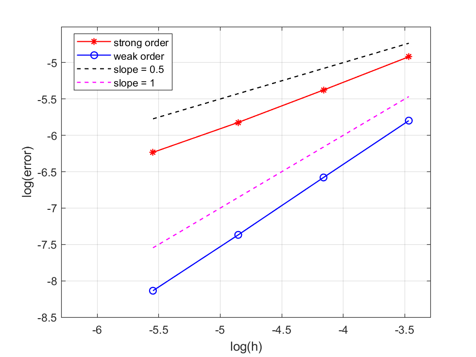
Figure 1: Convergence order in $\log-\log$ scale

7 Conclusion and Discussion

In this paper, we investigated the optimal weak convergence order for an FEM approximation to a stochastic Allen-Cahn equation driven by multiplicative white noise. We first constructed an auxiliary equation based on the splitting-up technique and derived the strong convergence order of 1 in time between the auxiliary and exact solutions. Then, we analyzed the weak errors between the FEM approximation and the exact solution and obtained the optimal weak convergence order in space.

It is well known that high-dimensional SPDEs driven by space-time white noise are generally ill-posed. Consequently, the results presented in this paper do not extend to the high-dimensional stochastic Allen-Cahn equation driven by multiplicative noise. We plan to address this challenge in future work by applying the methodologies developed in this paper.

Compliance with Ethical Standards

The authors declare that there are no conflicts of interest.

References

- \bibcommenthead
- Cai et al. [2024] Cai, M., Gan, S., Wang, X.: Weak approximations of stochastic partial differential equations with fractional noise. J. Comput. Math. 42(3), 735–754 (2024) https://doi.org/10.4208/jcm.2203-m2021-0194
- Cao et al. [2020] Cao, Y., Hong, J., Liu, Z.: Well-posedness and finite element approximations for elliptic SPDEs with Gaussian noises. Commun. Math. Res. 36(2), 113–127 (2020) https://doi.org/10.4208/cmr.2020-0006
- Chai et al. [2018] Chai, S., Cao, Y., Zou, Y., Zhao, W.: Conforming finite element methods for the stochastic Cahn-Hilliard-Cook equation. Appl. Numer. Math. 124, 44–56 (2018) https://doi.org/10.1016/j.apnum.2017.09.010
- Jentzen and Kloeden [2009] Jentzen, A., Kloeden, P.E.: The numerical approximation of stochastic partial differential equations. Milan J. Math. 77, 205–244 (2009) https://doi.org/10.1007/s00032-009-0100-0
- Lord and Tambue [2013] Lord, G.J., Tambue, A.: Stochastic exponential integrators for the finite element discretization of SPDEs for multiplicative and additive noise. IMA J. Numer. Anal. 33(2), 515–543 (2013) https://doi.org/10.1093/imanum/drr059
- Zhang et al. [2022] Zhang, F., Zou, Y., Chai, S., Zhang, R., Cao, Y.: Splitting-up spectral method for nonlinear filtering problems with correlation noises. J. Sci. Comput. 93(1), 25–24 (2022) https://doi.org/10.1007/s10915-022-01994-6
- Zhang et al. [2024] Zhang, F., Zou, Y., Chai, S., Cao, Y.: Numerical analysis of a time discretized method for nonlinear filtering problem with Lévy process observations. Adv. Comput. Math. 50(4), 73–32 (2024) https://doi.org/10.1007/s10444-024-10169-w
- Andersson and Larsson [2016] Andersson, A., Larsson, S.: Weak convergence for a spatial approximation of the nonlinear stochastic heat equation. Math. Comp. 85(299), 1335–1358 (2016) https://doi.org/10.1090/mcom/3016
- Debussche [2011] Debussche, A.: Weak approximation of stochastic partial differential equations: the nonlinear case. Math. Comp. 80(273), 89–117 (2011) https://doi.org/10.1090/S0025-5718-2010-02395-6
- Kovács et al. [2012] Kovács, M., Larsson, S., Lindgren, F.: Weak convergence of finite element approximations of linear stochastic evolution equations with additive noise. BIT 52(1), 85–108 (2012) https://doi.org/10.1007/s10543-011-0344-2
- Kruse [2014] Kruse, R.: Strong and Weak Approximation of Semilinear Stochastic Evolution Equations. Lecture Notes in Mathematics, vol. 2093, p. 177 (2014). https://doi.org/10.1007/978-3-319-02231-4 . https://doi.org/10.1007/978-3-319-02231-4
- Yan [2005] Yan, Y.: Galerkin finite element methods for stochastic parabolic partial differential equations. SIAM J. Numer. Anal. 43(4), 1363–1384 (2005) https://doi.org/10.1137/040605278
- Furihata et al. [2018] Furihata, D., Kovács, M., Larsson, S., Lindgren, F.: Strong convergence of a fully discrete finite element approximation of the stochastic Cahn-Hilliard equation. SIAM J. Numer. Anal. 56(2), 708–731 (2018) https://doi.org/10.1137/17M1121627
- Hutzenthaler and Jentzen [2020] Hutzenthaler, M., Jentzen, A.: On a perturbation theory and on strong convergence rates for stochastic ordinary and partial differential equations with nonglobally monotone coefficients. Ann. Probab. 48(1), 53–93 (2020) https://doi.org/10.1214/19-AOP1345
- Jentzen et al. [2020] Jentzen, A., Lindner, F., Puvsnik, P.: Exponential moment bounds and strong convergence rates for tamed-truncated numerical approximations of stochastic convolutions. Numer. Algorithms 85(4), 1447–1473 (2020) https://doi.org/10.1007/s11075-019-00871-y
- Qi et al. [2023] Qi, X., Zhang, Y., Xu, C.: An efficient approximation to the stochastic Allen-Cahn equation with random diffusion coefficient field and multiplicative noise. Adv. Comput. Math. 49(5), 73–24 (2023) https://doi.org/10.1007/s10444-023-10072-w
- Cerrai [2003] Cerrai, S.: Stochastic reaction-diffusion systems with multiplicative noise and non-Lipschitz reaction term. Probab. Theory Related Fields 125(2), 271–304 (2003) https://doi.org/10.1007/s00440-002-0230-6
- Kovács et al. [2015] Kovács, M., Larsson, S., Lindgren, F.: On the backward Euler approximation of the stochastic Allen-Cahn equation. J. Appl. Probab. 52(2), 323–338 (2015) https://doi.org/%****␣sn-article.bbl␣Line␣325␣****10.1239/jap/1437658601
- Kovács et al. [2018] Kovács, M., Larsson, S., Lindgren, F.: On the discretisation in time of the stochastic Allen-Cahn equation. Math. Nachr. 291(5-6), 966–995 (2018) https://doi.org/10.1002/mana.201600283
- Bréhier et al. [2019] Bréhier, C.-E., Cui, J., Hong, J.: Strong convergence rates of semidiscrete splitting approximations for the stochastic Allen-Cahn equation. IMA J. Numer. Anal. 39(4), 2096–2134 (2019) https://doi.org/10.1093/imanum/dry052
- Bréhier and Goudenège [2019] Bréhier, C.-E., Goudenège, L.: Analysis of some splitting schemes for the stochastic Allen-Cahn equation. Discrete Contin. Dyn. Syst. Ser. B 24(8), 4169–4190 (2019) https://doi.org/10.3934/dcdsb.2019077
- Qi and Wang [2019] Qi, R., Wang, X.: Optimal error estimates of Galerkin finite element methods for stochastic Allen-Cahn equation with additive noise. J. Sci. Comput. 80(2), 1171–1194 (2019) https://doi.org/10.1007/s10915-019-00973-8
- Wang [2020] Wang, X.: An efficient explicit full-discrete scheme for strong approximation of stochastic Allen-Cahn equation. Stochastic Process. Appl. 130(10), 6271–6299 (2020) https://doi.org/10.1016/j.spa.2020.05.011
- Liu and Qiao [2021] Liu, Z., Qiao, Z.: Strong approximation of monotone stochastic partial differential equations driven by multiplicative noise. Stoch. Partial Differ. Equ. Anal. Comput. 9(3), 559–602 (2021) https://doi.org/10.1007/s40072-020-00179-2
- Huang and Shen [2023] Huang, C., Shen, J.: Stability and convergence analysis of a fully discrete semi-implicit scheme for stochastic Allen-Cahn equations with multiplicative noise. Math. Comp. 92(344), 2685–2713 (2023) https://doi.org/10.1090/mcom/3846
- Yang et al. [2024] Yang, X., Zhao, W., Zhao, W.: Optimal error estimates of a discontinuous Galerkin method for stochastic Allen-Cahn equation driven by multiplicative noise. Commun. Comput. Phys. 36(1), 133–159 (2024)
- Kloeden and Platen [1992] Kloeden, P.E., Platen, E.: Numerical Solution of Stochastic Differential Equations. Applications of Mathematics (New York), vol. 23, p. 632 (1992). https://doi.org/10.1007/978-3-662-12616-5 . https://doi.org/10.1007/978-3-662-12616-5
- Milstein and Tretyakov [2004] Milstein, G.N., Tretyakov, M.V.: Stochastic Numerics for Mathematical Physics. Scientific Computation, p. 594 (2004). https://doi.org/%****␣sn-article.bbl␣Line␣475␣****10.1007/978-3-662-10063-9 . https://doi.org/10.1007/978-3-662-10063-9
- Bréhier et al. [2018] Bréhier, C.-E., Hairer, M., Stuart, A.M.: Weak error estimates for trajectories of SPDEs under spectral Galerkin discretization. J. Comput. Math. 36(2), 159–182 (2018) https://doi.org/10.4208/jcm.1607-m2016-0539
- Bréhier and Debussche [2018] Bréhier, C.-E., Debussche, A.: Kolmogorov equations and weak order analysis for SPDEs with nonlinear diffusion coefficient. J. Math. Pures Appl. (9) 119, 193–254 (2018) https://doi.org/10.1016/j.matpur.2018.08.010
- Jacobe de Naurois et al. [2021] Naurois, L., Jentzen, A., Welti, T.: Weak convergence rates for spatial spectral Galerkin approximations of semilinear stochastic wave equations with multiplicative noise. Appl. Math. Optim. 84, 1187–1217 (2021) https://doi.org/10.1007/s00245-020-09744-6
- Wang and Gan [2013] Wang, X., Gan, S.: Weak convergence analysis of the linear implicit Euler method for semilinear stochastic partial differential equations with additive noise. J. Math. Anal. Appl. 398(1), 151–169 (2013) https://doi.org/10.1016/j.jmaa.2012.08.038
- Conus et al. [2019] Conus, D., Jentzen, A., Kurniawan, R.: Weak convergence rates of spectral Galerkin approximations for SPDEs with nonlinear diffusion coefficients. Ann. Appl. Probab. 29(2), 653–716 (2019) https://doi.org/10.1214/17-AAP1352
- Jentzen and Kurniawan [2021] Jentzen, A., Kurniawan, R.: Weak convergence rates for Euler-type approximations of semilinear stochastic evolution equations with nonlinear diffusion coefficients. Found. Comput. Math. 21(2), 445–536 (2021) https://doi.org/10.1007/s10208-020-09448-x
- Andersson et al. [2016] Andersson, A., Kruse, R., Larsson, S.: Duality in refined Sobolev-Malliavin spaces and weak approximation of SPDE. Stoch. Partial Differ. Equ. Anal. Comput. 4(1), 113–149 (2016) https://doi.org/10.1007/s40072-015-0065-7
- Wang [2016] Wang, X.: Weak error estimates of the exponential Euler scheme for semi-linear SPDEs without Malliavin calculus. Discrete Contin. Dyn. Syst. 36(1), 481–497 (2016) https://doi.org/10.3934/dcds.2016.36.481
- Cui and Hong [2019] Cui, J., Hong, J.: Strong and weak convergence rates of a spatial approximation for stochastic partial differential equation with one-sided Lipschitz coefficient. SIAM J. Numer. Anal. 57(4), 1815–1841 (2019) https://doi.org/10.1137/18M1215554
- Cui et al. [2021] Cui, J., Hong, J., Sun, L.: Weak convergence and invariant measure of a full discretization for parabolic SPDEs with non-globally Lipschitz coefficients. Stochastic Process. Appl. 134, 55–93 (2021) https://doi.org/10.1016/j.spa.2020.12.003
- Cai et al. [2021] Cai, M., Gan, S., Wang, X.: Weak convergence rates for an explicit full-discretization of stochastic Allen-Cahn equation with additive noise. J. Sci. Comput. 86(3), 34–30 (2021) https://doi.org/10.1007/s10915-020-01378-8
- Da Prato et al. [2019] Da Prato, G., Jentzen, A., Röckner, M.: A mild Itô formula for SPDEs. Trans. Amer. Math. Soc. 372(6), 3755–3807 (2019) https://doi.org/10.1090/tran/7165
- Da Prato and Zabczyk [2014] Da Prato, G., Zabczyk, J.: Stochastic Equations in Infinite Dimensions, 2nd edn. Encyclopedia of Mathematics and its Applications, vol. 152, p. 493 (2014). https://doi.org/10.1017/CBO9781107295513 . https://doi.org/10.1017/CBO9781107295513
- Thomée [2006] Thomée, V.: Galerkin Finite Element Methods for Parabolic Problems, 2nd edn. Springer Series in Computational Mathematics, vol. 25, p. 370 (2006)
- Gawarecki and Mandrekar [2011] Gawarecki, L., Mandrekar, V.: Stochastic Differential Equations in Infinite Dimensions with Applications to Stochastic Partial Differential Equations. Probability and its Applications (New York), p. 291 (2011). https://doi.org/10.1007/978-3-642-16194-0 . https://doi.org/10.1007/978-3-642-16194-0
- León and Nualart [1998] León, J.A., Nualart, D.: Stochastic evolution equations with random generators. Ann. Probab. 26(1), 149–186 (1998) https://doi.org/10.1214/aop/1022855415
- Higham et al. [2002] Higham, D.J., Mao, X., Stuart, A.M.: Strong convergence of Euler-type methods for nonlinear stochastic differential equations. SIAM J. Numer. Anal. 40(3), 1041–1063 (2002) https://doi.org/10.1137/S0036142901389530
- Bréhier and Goudenège [2020] Bréhier, C.-E., Goudenège, L.: Weak convergence rates of splitting schemes for the stochastic Allen-Cahn equation. BIT 60(3), 543–582 (2020) https://doi.org/10.1007/s10543-019-00788-x