A novel numerical method for mean field stochastic differential equation

Abstract

In this paper, we propose a novel method to approximate the mean field stochastic differential equation by means of approximating the density function via Fokker-Planck equation. We construct a well-posed truncated Fokker-Planck equation whose solution is an approximation to the density function of solution to the mean field stochastic differential equation. We also apply finite difference method to approximate the truncated Fokker-Planck equation and derive error estimates. We use the numerical density function to replace the true measure in mean field stochastic differential equation and set up a stochastic differential equation to approximate the mean field one. Meanwhile, we derive the corresponding error estimates. Finally, we present several numerical experiments to illustrate the theoretical analysis.

AMS Classification]65C30, 82C31, 60H35, 65N06

1 Introduction

Stochastic differential equation (SDE for short) is a fundamental tool for modeling the evolution of various phenomena in different fields involving noise, cf. finance [1], chemical reaction [2] and environment science [3]. The mean field SDE, whose coefficient functions depend on the law of the solution, plays an important role in many fields: the Hodgkin-Huxley model for neuron activation in neuroscience [4], the Patlak-Keller-Segel equations in biology and chemistry [5, 6] and the Atlas models for equity markets in financial mathematics [7, 8].

In recent years, numerical approximations to the mean field SDE have attracted many attentions. Its main idea is to apply an interactive particle system to approximate the mean field SDE and then use an empirical measure to approach the joint distribution of particles. Therefore, the interactive particle system is usually transformed to a high dimensional SDE and various effective numerical methods can be applied to set up numerical schemes [9, 10, 11, 12]. Belomestny and Schoenmakers [13] proposed a projection-based particle method. Liu [14] proposed three numerical schemes and studied the convergence rate for the first one. Error estimates to the particle method showed that enlarging particle number improves the approximate accuracy. However, the simulation for empirical measure with a large number of particles is extremely costly. To overcome this difficulty, a random batch method was recently proposed and analyzed in [15, 16, 17, 18], which was designed to parallel simulate several small particle systems at each iteration step. This method largely reduced the computational complexity but raise the approximate error if the batch number is small.

In this paper, we will propose a novel method for a class of mean field SDEs based upon Fokker-Planck equation. In fact, the density function of the solution to a mean field SDE satisfies a nonlinear Fokker-Planck equation. Then we apply a finite difference method to the Fokker-Planck equation to obtain an approximate density function. Afterwards, we use the approximate density function to replace the true density function and transform the mean field SDE to an SDE, which can be easily solved by many numerical methods. Comparing with the particle method, our’s avoids a great amount simulations of high dimensional sample trajectories for determining the empirical measure. Instead, we numerically solve a deterministic Fokker-Planck equation, which results in a high precision approximate density function. In order to observe dynamical behavior of sample trajectory of a particle, one need to solve a high dimensional SDE if using interactive particle system to approximate the mean field SDE. However, we only need to solve an SDE after getting an approximate density function.

Now, we describe our method in more details. We first truncate the whole $\mathbb{R}^{d}$ space on to a bounded domain and construct a truncated Fokker-Planck equation equipped with a homogeneous Dirichlet boundary condition. Then, we apply an explicit-implicit difference scheme to approach the truncated equation to obtain a numerical density function. We replace the true density function in the mean field SDE with the approximate one, and hence obtain an SDE, with which we can easily simulate the approximate trajectories of the mean field SDE. Meanwhile, we also investigate corresponding error estimates.

The organization of this paper is as follows. In Section 2, we introduce a class of mean field SDEs and assumptions. In Section 3, we construct a truncated Fokker-Planck equation and apply an effective numerical method to approximate the density function. Based on the solution to the truncated Fokker-Planck equation, we construct an SDE to approximate the mean field SDE and investigate the corresponding error estimate. In Section 4, we construct an auxiliary SDE in terms of the numerical density function to approximate the mean field SDE. Then, we apply Euler-Maruyama method to solve this SDE and provide error estimates. In Section 5, We present some numerical experiments to illustrate the effectiveness of our method.

2 Preliminary

In this section, we introduce a class of mean field SDEs and some assumptions.

Let $d>0$ be an integer and $(\mathbb{R}^{d},|\cdot|)$ be a $d$-dimensional Euclidean space. By $|\cdot|_{F}$ we denote the Frobenius norm of a matrix. Let $C^{2}_{0}(\mathbb{R}^{d})$ be a space of twice continuously differentiable functions with compact support. For any integer $k\geq 0$, denote by $H^{k}(\mathbb{R}^{d})$ the standard Sobolev space, where $H^{0}(\mathbb{R}^{d})=L^{2}(\mathbb{R}^{d})$.

Let $T>0$ be a real number and $(\Omega,\mathcal{F},\mathbb{P})$ be a probability space. Denote by $W(t)$ $(t\in[0,T])$ an $m$-dimensional standard Brownian motion. By $\mathcal{P}(\mathbb{R}^{d})$ we denote the set of all probability measures on $\mathbb{R}^{d}$ and define a subset

$$\mathcal{P}_{2}(\mathbb{R}^{d})=\left\{\mu\in\mathcal{P}(\mathbb{R}^{d}):\int_{\mathbb{R}^{d}}|x|^{2}\mu(dx)<\infty\right\}.$$

Let $L^{2}(\Omega)$ be a space of $\mathbb{R}^{d}$-valued, $\mathcal{F}$ measurable random variables $X$ satisfying $E|X|^{2}<\infty$. By $\mathcal{L}_{X}$ we denote the law of $X\in L^{2}(\Omega)$.

Consider a class of mean field SDEs

$$dX(t)=F(t,X(t),\mathcal{L}_{X(t)})dt+\sigma(t,X(t))dW(t),\quad X(0)=X_{0}\in L^{2}(\Omega).$$ (1)

Define a filtration $\mathcal{F}_{t}=\sigma(X_{0},W(s),0\leq s\leq t)$. By abbreviation, let $\mu_{t}=\mathcal{L}_{X(t)}$ $(0\leq t\leq T)$ denote a family of laws of solution $X(t)$ to (1).

We assume

• the function $K=(K_{1},\cdots,K_{d})^{T}:[0,T]\times\mathbb{R}^{d}\times\mathbb{R}^{d}\to\mathbb{R}^{d}$ together with its derivatives up to second order are bounded and continuous. Furthermore, there exists a constant $L>0$ such that $\int_{\mathbb{R}^{d}}|K(t,x,y)|^{2}dy\leq L$ for all $(t,x)$.

• $F=(F_{1},\cdots,F_{d})^{T}:[0,T]\times\mathbb{R}^{d}\times\mathcal{P}(\mathbb{R}^{d})\to\mathbb{R}^{d}$ is defined as

  $$F(t,x,\mu_{t})=f(t,x)+\int_{\mathbb{R}^{d}}K(t,x,y)\mu_{t}(dy),$$

  where $f=(f_{1},\cdots,f_{d})^{T}:[0,T]\times\mathbb{R}^{d}\to\mathbb{R}^{d}$ is twice continuously differentiable with bounded first and seconde derivatives.

• $\sigma:[0,T]\times\mathbb{R}^{d}\to\mathbb{R}^{d\times m}$ is twice continuously differentiable with bounded first and second derivatives.

From (A2) and (A3), it follows that there exist a constant $L>0$ such that

$$|f(t,x)-f(t,\bar{x})|+|\sigma(t,{x})-\sigma(t,\bar{x})|_{F} \leq L|x-\bar{x}|,\quad\forall t\in[0,T],\ x,\bar{x}\in\mathbb{R}^{d}.$$ (2)

Under above three assumptions and by [19, 20], (1) has a unique solution $X(t)$ satisfying

$$E|X(t)|^{2}\leq L(1+E|X_{0}|^{2}),\quad\forall t\in[0,T].$$ (3)

Generally speaking, the existing numerical methods for approximating the mean field SDE are based on converting (1) to an interacting particle system, where the true measure is replaced by an empirical measure, which is a linear combination of point measures and is independently simulated by Monte Carlo method. Then, the interacting particle system is governed by a high dimensional SDE and many numerical methods can be applied. However, in order to get a high-accuracy empirical measure, the numbers of particles and sample trajectories should be extremely enlarged, which involves high computation complexity.

In this paper, we will propose a completely different method from the particle method to approach (1). In fact, the density function of the solution to (1) satisfies a deterministic nonlinear Fokker-Planck equation. Our strategy is to apply finite difference method to solve the nonlinear Fokker-Planck equation so as to obtain an approximate density function, which helps us to transform (1) to an SDE. By virtue of the classical theory on numerical partial differential equation (PDE for short), we obtain an approximate density function with desired precision, and then set up a high-accuracy approximation to (1). Compared to Monte Carlo simulation, our method reduces computation complexity while approximating the law of solution and accelerates the procedure of solving (1).

3 A nonlinear Fokker-Planck equation and the approximation

In this section, we first derive a nonlinear Fokker-Planck equation which characterizes the development of the density function of solution to mean field SDE (1). Then, we truncate the nonlinear Fokker-Planck onto a bounded domain and assign a homogeneous Dirichlet boundary value condition to construct an approximate equation. Afterward, we apply an explicit-implicit finite difference method to set up a fully discretized scheme for the truncated equation. Based on the approximate density function we construct an SDE to approximate the mean field SDE (6). We will derive error estimates between the solutions to the approximate SDE and the original mean field SDE.

3.1 A nonlinear Fokker-Planck equation

Denote by $p(t,x)$ the density function of the solution $X(t)$ to mean field SDE (6). Without loss of generality, we assume $p(t,\cdot)\in H^{2}(\mathbb{R}^{d})$ and $p\geq 0$. Thus, we have $\mu_{t}(dx)=p(t,x)dx$. Let $p_{0}(x)$ be the density function of $X_{0}$. From (3), it follows that

$$\int_{\mathbb{R}^{d}}|x|^{2}p(t,x)dx\leq C(1+\int_{\mathbb{R}^{d}}|x|^{2}p_{0}(x)dx)<+\infty,$$ (4)

which implies $p(t,x)=o(\frac{1}{|x|^{3}})$ as $x\to\infty$.

Now, we are already to derive a nonlinear Fokker-Planck equation. For any $\phi\in C^{2}_{0}(\mathbb{R}^{d})$, let $Y(t)=\phi(X(t))$, then

$$E(Y(t))=\int_{\mathbb{R}^{d}}p(t,x)\phi(x)dx.$$ (5)

Thus, (1) equivalently becomes

$$dX(t)=f(t,X(t))dt+\int_{\mathbb{R}^{d}}K(t,X(t),y)p(t,y)dydt+\sigma(t,X(t))dW(t).$$ (6)

By Itó’s formula, we have

$$\phi(X(t))=\phi(X(0))+\int_{0}^{t}L_{\mu_{s}}\phi(s,X(s))ds+\int_{0}^{t}(\bigtriangledown\phi(X(s)))^{T}\sigma(s,X(s))dW(s),$$ (7)

where

$$L_{\mu_{t}}\phi(t,x)=\sum_{i=1}^{d}\Big{(}f_{i}(t,x)+\int_{\mathbb{R}^{d}}K_{i}(t,x,y)p(t,y)dy\Big{)}\frac{\partial\phi(x)}{\partial x_{i}}+\frac{1}{2}\sum_{i,j=1}^{d}a_{ij}(t,x)\frac{\partial^{2}\phi(x)}{\partial x_{i}\partial x_{j}}.$$

Here $A=(a_{ij}):=\sigma\sigma^{T}$ is a symmetric matrix-valued function. Take expectations on both sides of (7) and apply the formula of integration by parts, then we get

$$\int_{\mathbb{R}^{d}}p(t,x)\phi(x)dx=\int_{\mathbb{R}^{d}}p_{0}(x)\phi(x)dx$$

$$\quad-\int_{\mathbb{R}^{d}}\!\sum_{i=1}^{d}\!\int_{0}^{t}\frac{\partial[(f_{i}(s,x)\!+\!\int_{\mathbb{R}^{d}}K_{i}(s,x,y)p(s,y)dy)p(s,x)]}{\partial x_{i}}ds\phi(x)dx$$

$$\quad+\frac{1}{2}\int_{\mathbb{R}^{d}}\sum_{i,j=1}^{d}\int_{0}^{t}\frac{\partial^{2}[a_{ij}(s,x)p(s,x)]}{\partial x_{i}\partial x_{j}}ds\phi(x)dx.$$

Since $C_{0}^{2}(\mathbb{R}^{d})$ is dense in $L^{2}(\mathbb{R}^{d})$, we obtain

$$p(t,x)= p_{0}(x)-\sum_{i=1}^{d}\int_{0}^{t}\frac{\partial[(f_{i}(s,x)+\int_{\mathbb{R}^{d}}K_{i}(s,x,y)p(s,y)dy)p(s,x)]}{\partial x_{i}}ds$$ (8)

$$+\frac{1}{2}\sum_{i,j=1}^{d}\int_{0}^{t}\frac{\partial^{2}[a_{ij}(s,x)p(s,x)]}{\partial x_{i}\partial x_{j}}ds.$$

Notice that the functions $f_{i}$, $K_{i}$ and $a_{ij}$ are continuous with respect to $t$, the solution $p$ of above equation is continuously differentiable with respect to $t$. Thus, we obtain a nonlinear Fokker-Planck equation [21, 22]

$$\frac{\partial p}{\partial t}=-\sum_{i=1}^{d}\frac{\partial[(f_{i}+\int_{\mathbb{R}^{d}}K_{i}(\cdot,\cdot,y)p(\cdot,y)dy)p]}{\partial x_{i}}+\frac{1}{2}\sum_{i,j=1}^{d}\frac{\partial^{2}[a_{ij}p]}{\partial x_{i}\partial x_{j}},$$ (9)

with initial value condition $p(0,x)=p_{0}(x)$.

In order to ensure the well-posedness of (9), we also assume

• There exist two constants $0<\gamma_{1}\leq\gamma_{2}$ such that

  $$\gamma_{1}|y|^{2}\leq y^{T}A(t,x)y\leq\gamma_{2}|y|^{2},\quad\forall t\in[0,T],x,y\in\mathbb{R}^{d}.$$

Under (A1)-(A4), the well-posedness and regularity of solution to autonomous nonlinear Fokker-Planck equation have been established [22], which may not be directly applied to the non-autonomous case. However, we focus on constructing a new numerical method to approximate the mean field SED (6) with the help of a solution to (9). In fact, the density function $p(t,x)$ is a solution to (9) and hence we only assume that $p$ is the unique solution without proof.

3.2 A numerical approximation to nonlinear Fokker-Planck equation

In order to approximate the nonlinear Fokker-Planck equation (9), we first truncate $\mathbb{R}^{d}$ to a bounded domain $\mathcal{D}=(-\alpha,\alpha)^{d}$ for some $\alpha>0$. Then we construct a truncated equation on $[0,T]\times\mathcal{D}$ to approximate (9)

$$\frac{\partial p_{\mathcal{D}}}{\partial t}=-\sum_{i=1}^{d}\frac{\partial[(f_{i}+\int_{\mathcal{D}}K_{i}(\cdot,\cdot,y)p_{\mathcal{D}}(\cdot,y)dy)p_{\mathcal{D}}]}{\partial x_{i}}+\frac{1}{2}\sum_{i,j=1}^{d}\frac{\partial^{2}[a_{ij}p_{\mathcal{D}}]}{\partial x_{i}\partial x_{j}}=$$ (10)

$$-\sum_{i=1}^{d}\frac{\partial[(f_{i}\!+\!\int_{\mathcal{D}}K_{i}(\cdot,\cdot,y)p_{\mathcal{D}}(\cdot,y)dy)p_{\mathcal{D}}]}{\partial x_{i}}\!+\!\frac{1}{2}\sum_{i=1}^{d}\frac{\partial^{2}[a_{ii}p_{\mathcal{D}}]}{\partial x_{i}^{2}}\!+\!\frac{1}{2}\sum_{i\not=j=1}^{d}\frac{\partial^{2}[a_{ij}p_{\mathcal{D}}]}{\partial x_{i}\partial x_{j}},$$

with initial-boundary value condition

$$p_{\mathcal{D}}(0,x)=p_{0}|_{{\mathcal{D}}}(x)\text{ for }x\in{\mathcal{D}},\quad p_{\mathcal{D}}(t,x)=0\text{ for }t\in(0,T),\ x\in\partial{\mathcal{D}}.$$ (11)

The unique existence and regularity estimates of the solution to (10)-(11) are interesting problems, but it is not the main task of this paper. Hence, we assume that the initial-boundary value problem (10)-(11) has a unique positive solution $p_{\mathcal{D}}(t,\cdot)\in H^{2}({\mathcal{D}})\cap H_{0}^{1}(\mathcal{D})$. Then, $p_{\mathcal{D}}$ is an approximation to $p|_{\mathcal{D}}$ and $p_{\mathcal{D}}\to p$ as $\alpha\to\infty$ in some a suitable space, which will be described in detail later.

Now, we study a finite difference approximation to (10). For any integer $N>0$, let $\kappa=\frac{T}{N}$ be a time step size and $t_{n}=n\kappa$ $(n=0,1,\cdots,N)$ be partition nodes. For any integer $M>0$, define two index sets

$$\mathbb{Z}_{M}=\{k\in Z^{d}:|k_{i}|\leq M,i=1,\cdots,d\},\quad\Theta_{M}=\mathbb{Z}_{M}\setminus\mathbb{Z}_{M-1}.$$

Let $h=\frac{\alpha}{M}$ be a spatial meshsize and $x^{k}=hk$, $k\in\mathbb{Z}_{M}$, be partition nodes inside domain $\mathcal{D}$. Define ${D}_{k}=[x_{k_{1}},x_{k_{1}+1}]\times\cdots\times[x_{k_{d}},x_{k_{d}+1}]$, then $\{D_{k}:k\in\mathbb{Z}_{M},k_{i}\leq M-1,i=1,\cdots,d\}$ is a uniform partition of ${\mathcal{D}}$.

Define a space of finite sequences

$$S_{\mathbb{Z}_{M}}^{0}=\left\{v_{\mathbb{Z}_{M}}=(v^{k})_{k\in\mathbb{Z}_{M}}\in\mathbb{R}^{\mathbb{Z}_{M}}:v^{k}=0~\text{for}~k\in\Theta_{M}\right\}$$

equipped with a discrete $L^{2}$-norm $\|v_{\mathbb{Z}_{M}}\|^{2}_{S^{0}_{\mathbb{Z}_{M}}}=\displaystyle\sum_{k\in\mathbb{Z}_{M}}|v^{k}|^{2}h^{d}.$

For any $1\leq i\leq d$, define a unit vector $\eta^{i}\in\mathbb{R}^{d}$ whose i-th component is equal to $1$. For any $n=0,1,\cdots,N$ and $k\in\mathbb{Z}_{M}$, let $f_{i}^{n,k}=f_{i}(t_{n},x^{k})$, $a_{ij}^{n,k}=a_{ij}(t_{n},x^{k})$ and $p^{n,k}_{{\mathcal{D}}}$ be an approximation to $p_{\mathcal{D}}(t_{n},x^{k})$. Denote a numerical integration by ${\mathcal{S}}_{i}^{n,k}=\displaystyle\sum_{s\in\mathbb{Z}_{M}}K_{i}(t_{n},x^{k},x^{s})p^{n,s}_{{\mathcal{D}}}h^{d}$. Now, we construct an explicit-implicit difference scheme to approximate (10)

$$\frac{p^{n+1,k}_{{\mathcal{D}}}-p^{n,k}_{{\mathcal{D}}}}{\kappa}$$ (12)

$$= -\sum_{i=1}^{d}\frac{(f_{i}^{n,k+\eta^{i}}+{\mathcal{S}}_{i}^{n,k+\eta^{i}})p^{n,k+\eta^{i}}_{{\mathcal{D}}}-(f_{i}^{n,k-\eta^{i}}+{\mathcal{S}}_{i}^{n,k-\eta^{i}})p^{n,k-\eta^{i}}_{{\mathcal{D}}}}{2h}$$

$$+\sum_{i=1}^{d}\frac{a_{ii}^{n+1,k+\eta^{i}}p^{n+1,k+\eta^{i}}_{{\mathcal{D}}}-2a_{ii}^{n+1,k}p^{n+1,k}_{{\mathcal{D}}}+a_{ii}^{n+1,k-\eta^{i}}p^{n+1,k-\eta^{i}}_{{\mathcal{D}}}}{2h^{2}}$$

$$+\sum_{i\neq j=1}^{d}\Big{(}\frac{a_{ij}^{n+1,k+\eta^{i}+\eta^{j}}p^{n+1,k+\eta^{i}+\eta^{j}}_{{\mathcal{D}}}-a_{ij}^{n+1,k+\eta^{i}-\eta^{j}}p^{n+1,k+\eta^{i}-\eta^{j}}_{{\mathcal{D}}}}{8h^{2}}$$

$$\quad\quad+\frac{-a_{ij}^{n+1,k-\eta^{i}+\eta^{j}}p^{n+1,k-\eta^{i}+\eta^{j}}_{{\mathcal{D}}}+a_{ij}^{n+1,k-\eta^{i}-\eta^{j}}p^{n+1,k-\eta^{i}-\eta^{j}}_{{\mathcal{D}}}}{8h^{2}}\Big{)}.$$

As $\kappa$ and $h$ are sufficiently small, we obtain a unique $p_{{\mathcal{D}},\mathbb{Z}_{M}}^{n+1}=(p^{n+1,k}_{{\mathcal{D}}})_{k\in\mathbb{Z}_{M}}\in S^{0}_{\mathbb{Z}_{M}}$ by solving linear equation (12) for any given $p_{{\mathcal{D}},\mathbb{Z}_{M}}^{n}=(p^{n,k}_{{\mathcal{D}}})_{k\in\mathbb{Z}_{M}}\in S^{0}_{\mathbb{Z}_{M}}$. Hence for a given initial value $(p_{{\mathcal{D}}}(0,x^{k}))_{k\in\mathbb{Z}_{M}}\in S^{0}_{\mathbb{Z}_{M}}$, we recursively solve (12) to get a numerical solution $p_{{\mathcal{D}},\mathbb{Z}_{M}}^{n}$ $(n=1,2,\cdots,N)$ to (10)-(11). The classical error analysis theorem [23] provides convergence property, which is summarized in next lemma and its proof is omitted.

Lemma 1.

Assume (A1)-(A4) hold. Let $p_{\mathcal{D}}$ and $p_{{\mathcal{D}},\mathbb{Z}_{M}}^{n}$ $(n=1,2,\cdots,N)$ be the real and numerical solutions to (10)-(11), respectively. Then, there exits a constant $C>0$ such that

$$\|(p_{\mathcal{D}}(t_{n},x^{k}))_{k\in\mathbb{Z}_{M}}-p_{{\mathcal{D}},\mathbb{Z}_{M}}^{n}\|_{S^{0}_{\mathbb{Z}_{M}}}\leq C(\kappa+h^{2}).$$

3.3 An approximation to the mean field equation

In this section, we apply the approximate density function $p_{\mathcal{D}}(t,x)$ to construct an SDE to approximate the mean field SDE (6). We also derive error estimates between their solutions.

Let $I_{\mathcal{D}}(x)$ be an indicator function on $\mathcal{D}$, i.e. $I_{\mathcal{D}}(x)=1$ if $x\in{\mathcal{D}}$ and $I_{\mathcal{D}}(x)=0$ otherwise. By $p_{\mathcal{D}}\cdot I_{\mathcal{D}}(x)$ we denote a function defined on the whole space $\mathbb{R}^{d}$, which can be regarded as the zero extension of $p_{\mathcal{D}}$. If no confusion occurs, we still use $p_{\mathcal{D}}$ to denote the extended function $p_{\mathcal{D}}\cdot I_{\mathcal{D}}(x)$. Furthermore, we also assume $p_{\mathcal{D}}$ together with its derivatives converges to the counterparts of the solution $p$ to (9) as $\alpha\to\infty$, i.e.

$$\Phi(\alpha):=\displaystyle\sup_{t\in[0,T]}\|p(t,\cdot)-p_{\mathcal{D}}(t,\cdot)\|_{L^{1}(\mathbb{R}^{d})}+\|p(t,\cdot)-p_{\mathcal{D}}(t,\cdot)\|_{H^{2}(\mathbb{R}^{d})}\to 0\text{ as }\alpha\to\infty.$$

Then there exists a constant $C>0$ such that for $t\in[0,T]$ and large $\alpha$

$$\int_{\mathcal{D}}p_{\mathcal{D}}(t,x)dx \leq\int_{\mathbb{R}^{d}}p(t,x)dx+\int_{\mathbb{R}^{d}}|p(t,x)-p_{\mathcal{D}}(t,x)|dx\leq 1+\Phi(\alpha)\leq C,$$ (13)

$$\|p_{\mathcal{D}}(t,\cdot)\|_{H^{2}(\mathcal{D})} \leq\|p(t,\cdot)\|_{H^{2}(\mathbb{R}^{d})}+\|p(t,\cdot)-p_{\mathcal{D}}(t,\cdot)\|_{H^{2}(\mathbb{R}^{d})}\leq C+\Phi(\alpha)\leq C.$$

We use the approximate density function $p_{\mathcal{D}}$ to replace the real density function $p$ in mean field SDE (6), and hence obtain an SDE

$$dX_{\mathcal{D}}(t)=f(t,X_{\mathcal{D}}(t))dt+\int_{\mathbb{R}^{d}}K(t,X_{\mathcal{D}}(t),y)p_{\mathcal{D}}(t,y)dydt+\sigma(t,X_{\mathcal{D}}(t))dW(t),$$ (14)

with the same initial value condition $X_{\mathcal{D}}(0)=X(0)$. Obviously, (14) is an approximation to the mean field SDE (6). Under assumptions (A1)-(A3), (14) has a unique solution $X_{\mathcal{D}}(t)$ satisfying a priori estimate, cf. [19]

$$E|X_{\mathcal{D}}(t)|^{2}\leq C(1+E|X_{0}|^{2}),\quad\forall t\in[0,T].$$ (15)

The next lemma investigates the error estimate between the solutions of mean field SDE (6) and SDE (14).

Lemma 2.

Assume (A1)-(A3) hold. Let $X(t)$ and $X_{\mathcal{D}}(t)$ be solutions of (6) and (14), respectively. Then, there holds

$$E|X(t)-X_{\mathcal{D}}(t)|^{2}\leq C\Phi^{2}(\alpha),\quad\forall t\in[0,T],$$

where $C=C(L,T)>0$ is a constant.

Proof.

According to (6) and (14), we have

$${X}(t)-{X}_{\mathcal{D}}(t)=\int_{0}^{t}f(s,{X}(s))-f(s,{X}_{\mathcal{D}}(s))ds$$

$$+\int_{0}^{t}\int_{\mathbb{R}^{d}}\!K(s,{X}(s),y){p}(s,y)-K(s,{X}_{\mathcal{D}}(s),y){p}_{\mathcal{D}}(s,y)dyds$$

$$+\int_{0}^{t}\sigma(s,{X}(s))-\sigma(s,{X}_{\mathcal{D}}(s))dW(s).$$

By Itó’s formula, we get

$$|{X}(t)-{X}_{\mathcal{D}}(t)|^{2}=2\int_{0}^{t}\langle{X}(s)-{X}_{\mathcal{D}}(s),f(s,{X}(s))-f(s,{X}_{\mathcal{D}}(s))\rangle ds$$

$$+2\int_{0}^{t}\langle{X}(s)-{X}_{\mathcal{D}}(s),\int_{\mathbb{R}^{d}}K(s,{X}(s),y){p}(s,y)-K(s,{X}_{\mathcal{D}}(s),y){p}_{\mathcal{D}}(s,y)dy\rangle ds$$

$$+\int_{0}^{t}\text{tr}[(\sigma(s,{X}(s))-\sigma(s,{X}_{\mathcal{D}}(s)))(\sigma(s,{X}(s))-\sigma(s,{X}_{\mathcal{D}}(s)))^{T}]ds$$

$$+2\int_{0}^{t}\langle{X}(s)-{X}_{\mathcal{D}}(s),(\sigma(s,{X}(s))-\sigma(s,{X}_{\mathcal{D}}(s))dW(s)\rangle.$$

Taking expectations on both sides of above equation and applying (2) and Cauchy-Schwarz inequality, we obtain

$$E|{X}(t)-{X}_{\mathcal{D}}(t)|^{2}=2E\int_{0}^{t}\langle{X}(s)-{X}_{\mathcal{D}}(s),f(s,{X}(s))-f(s,{X}_{\mathcal{D}}(s))\rangle ds$$

$$+2E\int_{0}^{t}\langle{X}(s)-{X}_{\mathcal{D}}(s),\int_{\mathbb{R}^{d}}K(s,{X}(s),y){p}(s,y)-K(s,{X}_{\mathcal{D}}(s),y){p}_{\mathcal{D}}(s,y)dy\rangle ds$$

$$+E\int_{0}^{t}\text{tr}[(\sigma(s,{X}(s))-\sigma(s,{X}_{\mathcal{D}}(s)))(\sigma(s,{X}(s))-\sigma(s,{X}_{\mathcal{D}}(s)))^{T}]ds$$

$$\leq 2E\int_{0}^{t}|{X}(s)-{X}_{\mathcal{D}}(s)|\cdot|f(s,{X}(s))-f(s,{X}_{\mathcal{D}}(s))|ds$$

$$+2E\int_{0}^{t}|{X}(s)-{X}_{\mathcal{D}}(s)|\cdot|\int_{\mathbb{R}^{d}}K(s,{X}(s),y){p}(s,y)-K(s,{X}_{\mathcal{D}}(s),y){p}_{\mathcal{D}}(s,y)dy|ds$$

$$+E\int_{0}^{t}|\sigma(s,{X}(s))-\sigma(s,{X}_{\mathcal{D}}(s))|_{F}^{2}ds$$

$$\leq 2E\int_{0}^{t}L|{X}(s)-{X}_{\mathcal{D}}(s)|^{2}ds+E\int_{0}^{t}|{X}(s)-{X}_{\mathcal{D}}(s)|^{2}ds$$

$$+E\int_{0}^{t}|\int_{\mathbb{R}^{d}}K(s,{X}(s),y){p}(s,y)-K(s,{X}_{\mathcal{D}}(s),y){p}_{\mathcal{D}}(s,y)dy|^{2}ds$$

$$+E\int_{0}^{t}L^{2}|{X}(s)-{X}_{\mathcal{D}}(s)|^{2}ds.$$

Noticing that

$$|\int_{\mathbb{R}^{d}}K(s,{X}(s),y){p}(s,y)-K(s,{X}_{\mathcal{D}}(s),y){p}_{\mathcal{D}}(s,y)dy|$$

$$\leq \int_{\mathbb{R}^{d}}|K(s,{X}(s),y)-K(s,{X}_{\mathcal{D}}(s),y)|p(s,y)dy$$

$$+\int_{\mathbb{R}^{d}}|K(s,{X}_{\mathcal{D}}(s),y)|\cdot|{p}(s,y)-{p}_{\mathcal{D}}(s,y)|dy$$

$$\leq L|{X}(s)-{X}_{\mathcal{D}}(s)|\int_{\mathbb{R}^{d}}p(s,y)dy+C\Phi(\alpha)\leq L|{X}(s)-{X}_{\mathcal{D}}(s)|+C\Phi(\alpha).$$

The above two inequalities imply

$$E|X(t)-{X}_{\mathcal{D}}(t)|^{2}\leq C(L)\int_{0}^{t}E|{X}(s)-{X}_{\mathcal{D}}(s)|^{2}ds+C(L)T\Phi^{2}(\alpha).$$

Then the proof follows from Gronwall’s inequality. ∎

4 A numerical approximation to the mean field SDE

In this section, based on the numerical solution to (10)-(11), we construct an auxiliary SDE to approximate (14) and investigate the corresponding error estimates. Then, we apply Euler-Maruyama method to the auxiliary SDE to set up a numerical scheme which is used to approximate the mean field SDE (6). Finally, we study the error estimates between the numerical solution and the exact solution of the mean field SDE.

4.1 An auxiliary SDE and error estimates

Define a piece-wise constant function $p_{\kappa,h}(t,x)={p}_{{\mathcal{D}}}^{n,k}$ for $(t,x)\in[t_{n},t_{n+1})\times D_{k}$ and extend its domain to $\mathbb{R}^{d}$ by $p_{\kappa,h}(t,x)=0$ for $x\in{\mathcal{D}}^{c}$. We replace the approximate density function $p_{\mathcal{D}}(t,x)$ in (14) by $p_{\kappa,h}(t,x)$, and then set up an auxiliary SDE for $t\in[0,T]$

$$d\hat{X}(t)=f(t,\hat{X}(t))dt+\int_{\mathbb{R}^{d}}K(t,\hat{X}(t),y)p_{\kappa,h}(t,x)dydt+\sigma(t,\hat{X}(t))dW(t),$$ (16)

with $\hat{X}(0)=X(0)$. Under assumptions (A1)-(A3), (16) has a unique solution $\hat{X}(t)$ which has second order moment estimate, cf. [19]

$$E|\hat{X}(t)|^{2}\leq C(1+E|X_{0}|^{2}),\quad\forall t\in[0,T],$$ (17)

where $C>0$ is a constant.

Lemma 3.

Assume (A1)-(A4) hold. Let $X_{\mathcal{D}}(t)$ and $\hat{X}(t)$ be solutions of (14) and (16), respectively. Then, there holds

$$E|X_{\mathcal{D}}(t)-\hat{X}(t)|^{2}\leq C(\kappa^{2}+h^{2}),\quad\forall t\in[0,T],$$

where $C=C(L,T)>0$ is a constant.

Proof.

(14) minus (16) yields

$$X_{\mathcal{D}}(t)-\hat{X}(t)= \int_{0}^{t}f(s,X_{\mathcal{D}}(s))-f(s,\hat{X}(s))ds$$

$$+\int_{0}^{t}\int_{\mathbb{R}^{d}}K(s,X_{\mathcal{D}}(s),y){p}_{\mathcal{D}}(s,y)-K(s,\hat{X}(s),y)p_{\kappa,h}(s,y)dyds$$

$$+\int_{0}^{t}\sigma(s,X_{\mathcal{D}}(s))-\sigma(s,\hat{X}(s))dW(s),$$

By Itó’s formula, we get

$$|X_{\mathcal{D}}(t)-\hat{X}(t)|^{2}=2\int_{0}^{t}\langle X_{\mathcal{D}}(s)-\hat{X}(s),f(s,{X}_{\mathcal{D}}(s))-f(s,\hat{X}(s))\rangle ds$$

$$+2\int_{0}^{t}\langle X_{\mathcal{D}}(s)-\hat{X}(s),\int_{\mathbb{R}^{d}}K(s,{X}_{\mathcal{D}}(s),y){p}_{\mathcal{D}}(s,y)-K(s,\hat{X}(s),y)p_{\kappa,h}(s,y)dy\rangle ds$$

$$+\int_{0}^{t}\text{tr}[(\sigma(s,X_{\mathcal{D}}(s))-\sigma(s,\hat{X}(s)))(\sigma(s,X_{\mathcal{D}}(s))-\sigma(s,\hat{X}(s)))^{T}]ds$$

$$+2\int_{0}^{t}\langle X_{\mathcal{D}}(s)-\hat{X}(s),(\sigma(s,X_{\mathcal{D}}(s))-\sigma(s,\hat{X}(s)))dW(s)\rangle.$$

Similar to the proof in Lemma 2 and by cauchy-schwarz inequality, we get

$$E|X_{\mathcal{D}}(t)-\hat{X}(t)|^{2}$$

$$\leq CE\int_{0}^{t}|X_{\mathcal{D}}(s)-\hat{X}(s)|^{2}ds$$

$$+E\int_{0}^{t}|\int_{\mathbb{R}^{d}}K(s,{X}_{\mathcal{D}}(s),y){p}_{\mathcal{D}}(s,y)-K(s,\hat{X}(s),y)p_{\kappa,h}(s,y)dy|^{2}ds$$

$$\leq CE\int_{0}^{t}|X_{\mathcal{D}}(s)-\hat{X}(s)|^{2}ds$$

$$+E\int_{0}^{t}2\big{(}\int_{\mathbb{R}^{d}}|K(s,{X}_{\mathcal{D}}(s),y)-K(s,\hat{X}(s),y)|{p}_{\mathcal{D}}(s,y)dy\big{)}^{2}ds$$

$$+E\int_{0}^{t}2\big{(}\int_{\mathbb{R}^{d}}|K(s,\hat{X}(s),y)|\cdot|{p}_{\mathcal{D}}(s,y)-p_{\kappa,h}(s,y)|dy\big{)}^{2}ds$$

$$\leq CE\int_{0}^{t}|X_{\mathcal{D}}(s)-\hat{X}(s)|^{2}ds$$

$$+E\int_{0}^{t}2L^{2}|{X}(s)-{X}_{\mathcal{D}}(s)|^{2}\big{(}\int_{\mathcal{D}}{p}_{\mathcal{D}}(s,y)dy\big{)}^{2}ds$$

$$+E\int_{0}^{t}2\int_{\mathbb{R}^{d}}|K(s,\hat{X}(s),y)|^{2}dy\int_{\mathcal{D}}|{p}_{\mathcal{D}}(s,y)-p_{\kappa,h}(s,y)|^{2}dyds,$$

where $C=C(L)>0$ is a constant.

By mean value theorem, Lemma 1 and (13), we have for any $n=0,1\cdots N-1$ and $s\in[t_{n},t_{n+1}]$

$$\int_{\mathcal{D}}|{p}_{\mathcal{D}}(s,y)-p_{\kappa,h}(s,y)|^{2}dy$$

$$= \sum_{k\in\mathbb{Z}_{M}}\int_{D_{k}}|{p}_{\mathcal{D}}(s,y)-{p}_{\mathcal{D}}^{n,k}|^{2}dy$$

$$\leq 2\sum_{k\in\mathbb{Z}_{M}}\int_{D_{k}}|{p}_{\mathcal{D}}(s,y)-{p}_{\mathcal{D}}(t_{n},x^{k})|^{2}dy+2\sum_{k\in\mathbb{Z}_{M}}\int_{D_{k}}|{p}_{\mathcal{D}}(t_{n},x^{k})-{p}_{\mathcal{D}}^{n,k}|^{2}dy$$

$$\leq 2\sum_{k\in\mathbb{Z}_{M}}\int_{D_{k}}|\frac{\partial p_{\mathcal{D}}(t_{n}^{\theta},y^{k}_{\theta})}{\partial t}(s-t_{n})+\sum_{i=1}^{d}\frac{\partial p_{\mathcal{D}}(t_{n}^{\theta},y^{k}_{\theta})}{\partial y_{i}}(y_{i}-x^{k}_{i})|^{2}dy$$

$$+2\|(p_{\mathcal{D}}(t_{n},x^{k}))_{k\in\mathbb{Z}_{M}}-p_{{\mathcal{D}},\mathbb{Z}_{M}}^{n}\|_{S^{0}_{\mathbb{Z}_{M}}}^{2}$$

$$\leq 2(d+1)\int_{\mathcal{D}}\kappa^{2}|\frac{\partial p_{\mathcal{D}}(t_{n}^{\theta},y^{k}_{\theta})}{\partial t}|^{2}dy+h^{2}\sum_{i=1}^{d}|\frac{\partial p_{\mathcal{D}}(t_{n}^{\theta},y^{k}_{\theta})}{\partial y_{i}}|^{2}dy+C(\kappa^{2}+h^{4})$$

$$\leq C(\kappa^{2}+h^{2}),$$

where $(t_{n}^{\theta},y^{k}_{\theta})=\theta(s,y)+(1-\theta)(t_{n},x^{k})$ and $C>0$ is a constant independent of $\kappa$ and $h$. The above two inequalities imply

$$E|X_{\mathcal{D}}(t)-\hat{X}(t)|^{2}\leq C(\kappa^{2}+h^{2})+C\int_{0}^{t}E|X_{\mathcal{D}}(s)-\hat{X}(s)|^{2}ds.$$

Then the proof follows from Gronwall’s inequality. ∎

4.2 A numerical approximation to the auxiliary SDE

In this section, we apply Euler-Maruyama method to auxiliary equation (16) to construct a numerical scheme for the original mean field SDE (1) and derive error estimates.

We take the same temporal step size $\kappa=\frac{T}{N}$ and $t_{n}=n\kappa$ $(n=0,1,\cdots,N)$ as in section 3.2 and apply Euler-Maruyama scheme for SDE (16)

$$\hat{X}^{n+1}= \hat{X}^{n}\!+\!f(t_{n},\hat{X}_{\kappa}^{n})\kappa\!+\!\kappa\!\int_{\mathbb{R}^{d}}\!K(t_{n},\hat{X}^{n},y)p_{\kappa,h}(t_{n},y)dy\!+\!\sigma(t_{n},\hat{X}^{n})\Delta W_{n}.$$ (18)

where $\Delta W_{n}=W(t_{n+1})-W(t_{n})$. From [24, 25, 26], it follows that

$$E|\hat{X}(t_{n})-\hat{X}^{n}|^{2}\leq C\kappa,\quad n=1,2,\cdots,N,$$ (19)

where $\hat{X}(t)$ is the solution of auxiliary equation (16). Specifically, if the function $\sigma$ is independent of $(t,x)$, where (18) is driven by additive noise, the convergence order for Euler-Maruyama method becomes of $1$, i.e.

$$E|\hat{X}(t_{n})-\hat{X}^{n}|^{2}\leq C\kappa^{2},\quad n=1,2,\cdots,N.$$ (20)

Now, we are ready to state and prove the main result in this paper.

Theorem 4.

Assume (A1)-(A4) hold. Let $X(t)$ and $\hat{X}^{n}$ $(n=0,1,\cdots,N)$ be solutions to (6) and (18), respectively. Then there exists a constant $C>0$ independent of $\kappa$ and $h$ such that

$$E|{X}(t_{n})-\hat{X}^{n}|^{2}\leq C\Phi^{2}(\alpha)+C(\kappa+h^{2}),\quad n=1,2,\cdots,N.$$

Furthermore, if the function $\sigma$ is independent of $(t,x)$, there holds

$$E|{X}(t_{n})-\hat{X}^{n}|^{2}\leq C\Phi^{2}(\alpha)+C(\kappa^{2}+h^{2}),\quad n=1,2,\cdots,N.$$

Proof.

Let ${X}_{\mathcal{D}}(t)$ and $\hat{X}(t)$ be solutions to (14) and (16), respectively. According to Lemmas 2 and 16 and estimate in (19), we have

$$E|{X}(t_{n})-\hat{X}^{n}|^{2}$$

$$\leq 3E|X(t_{n})-{X}_{\mathcal{D}}(t_{n})|^{2}+3E|{X}_{\mathcal{D}}(t_{n})-\hat{X}(t_{n})|^{2}+3E|\hat{X}(t_{n})-\hat{X}^{n}|^{2}$$

$$\leq C\Phi^{2}(\alpha)+C(\kappa^{2}+h^{2})+C\kappa$$

$$\leq C\Phi^{2}(\alpha)+C(\kappa+h^{2}).$$

The other estimate follows from a similar way. Thus, the proof is completed. ∎

5 Numerical experiments

In this section we will present three numerical experiments to illustrate the theoretical analysis.

Example 1.

Consider a mean field SDE driven by multiplicative noise

$$dX(t) =0.1(X(t)+\sin{t})dt+0.1\int_{\mathbb{R}^{d}}\frac{\sin y}{1+y^{2}}\mu_{t}(dy)dt+\frac{1}{\sqrt{10}}X(t)dW(t),$$ (21)

$$X(0) =X_{0}\sim N(0,1),$$

where $\mu_{t}={\mathcal{L}}_{X(t)}$.

The corresponding Fokker-Planck equation reads

$$\frac{\partial p(t,x)}{\partial t} =0.1\frac{\partial[(x+\sin{t}+\int_{\mathbb{R}}\frac{\sin y}{1+y^{2}}p(t,y)dy)p(t,x)]}{\partial x}+\frac{1}{5}\frac{\partial^{2}[x^{2}p(t,x)]}{\partial x^{2}}$$ (22)

and $p_{0}(x)=\frac{1}{\sqrt{2\pi}}e^{-x^{2}}$.

Take $[0,T]=[0,1]$ and $\mathcal{D}=[-6,6]$. We choose $\kappa_{0}=2^{-14}$ and $h_{0}=12\cdot 2^{-10}$ to calculate an approximate density function $p_{\mathcal{D},0}^{n,k}$ which is regarded as a referee exact solution to (22). Then, we select different time step sizes $\kappa=2^{-9},2^{-10},2^{-11},2^{-12}$ to approximate (22), to check the corresponding temporal error estimates and convergence orders, which are presented in Table. 2 and Fig. 2, respectively. Meanwhile, we take $h/12=2^{-8},2^{-7},2^{-6},2^{-5}$ to carry out numerical computation and detect spatial error estimates and convergence orders, see Table. 2 and Fig. 2, respectively.

Denote by $p_{\kappa_{0},h_{0}}(t,x)$ a continuous version of $p_{\mathcal{D},0}^{n,k}$ as defined at the beginning of Section 4.1. We simulate $10^{5}$ many sample trajectories using Euler-Maruyama scheme (18) for each step size $\kappa=2^{-9},2^{-10},2^{-11},2^{-12},2^{-14}$ to verify the error estimates and convergence orders, as shown in Table.  3 and Fig. 3.

The above results imply that the numerical computations for approximating PDE and SDE are effective and accurate. In order to show the validity of our method, we simulate the expectation and variance of the solution $X(t)$ to (21) using three different methods. First, we directly calculate the expectation and variance by virtue of the numerical density function, which are listed in the first line in Table. 4. Then, we use the computed $10^{4}$ sample trajectories to simulate the expectation and variance, see the second line in Table. 4. Finally, we apply particle method with $10^{3}$ particles and $10^{4}$ sample trajectories to approximate (21) and calculate expectation and variance, cf. the third line in Table. 4.

$\kappa$	error	order
$2^{-12}$	4.3019e-06	-
$2^{-11}$	1.0036e-05	1.2221
$2^{-10}$	2.1495e-05	1.0989
$2^{-9}$	4.4383e-05	1.0460

Table 1: Error and convergence order.

$h$	error	order
$0.0469$	2.1936e-05	-
$0.0938$	9.2028e-05	2.0688
$0.1875$	3.7104e-04	2.0114
$0.3750$	0.0015	1.9833

Table 2: Error and convergence order.

Figure 1: $\log-\log$ error.

Figure 2: $\log-\log$ error.

$\kappa$	error	order
$2^{-12}$	0.0081	-
$2^{-11}$	0.0128	0.5488
$2^{-10}$	0.0187	0.5683
$2^{-9}$	0.0277	0.5646

Table 3: Error and convergence order.

Figure 3: $\log-\log$ error.

	$E_{X}$	$V_{X}$
PDF method	0.0476	1.3305
Sample trajectory method	0.0474	1.3476
Particle method	0.0462	1.3381

Table 4: Expectation and variance.

Example 2.

Consider a $2$-dimensional mean field SDE driven by additive noise

$$dX(t)= 0.1\begin{pmatrix}\sqrt{(X_{1}(t))^{2}+(X_{2}(t))^{2}+0.4}\\ \sqrt{(X_{1}(t))^{2}+(X_{2}(t))^{2}+0.4}\end{pmatrix}dt+0.1\begin{pmatrix}\int_{\mathbb{R}^{2}}\frac{\sin y_{1}}{1+y_{1}^{2}}\frac{\sin y_{2}}{1+y_{2}^{2}}\mu_{t}(dy)\\ \int_{\mathbb{R}^{2}}\frac{\sin y_{1}}{1+y_{1}^{2}}\frac{\sin y_{2}}{1+y_{2}^{2}}\mu_{t}(dy)\end{pmatrix}dt$$ (23)

$$\!+\!\begin{pmatrix}\frac{2}{\sqrt{1}0}dW_{1}(t)+\frac{1}{\sqrt{1}0}dW_{2}(t)\\ \frac{1}{\sqrt{1}0}dW_{1}(t)+\frac{2}{\sqrt{1}0}dW_{2}(t)\end{pmatrix},$$

$$X(0)= (X_{0}^{1},X_{0}^{2})\overset{iid}{\sim}N(0,0.04).$$

The corresponding Fokker-Planck equation reads

$$\frac{\partial p}{\partial t}\!= -0.1\frac{\partial[(\sqrt{x_{1}^{2}+x_{2}^{2}+0.4})+\int_{\mathbb{R}^{2}}\frac{\sin y_{1}}{1+y_{1}^{2}}\frac{\sin y_{2}}{1+y_{2}^{2}}p(t,y_{1},y_{2})dy_{1}dy_{2}p]}{\partial x_{1}}+\frac{1}{4}\frac{\partial^{2}p}{\partial x_{1}^{2}}$$ (24)

$$\!-\!0.1\frac{\partial[\sqrt{x_{1}^{2}\!+\!x_{2}^{2}\!+\!0.4}\!+\!\int_{\mathbb{R}^{2}}\frac{\sin y_{1}}{1+y_{1}^{2}}\frac{\sin y_{2}}{1+y_{2}^{2}}p(t,y_{1},y_{2})dy_{1}dy_{2})p]}{\partial x_{2}}\!+\!\frac{1}{4}\frac{\partial^{2}p}{\partial x_{2}^{2}}\!+\!\frac{2}{5}\frac{\partial^{2}p}{\partial x_{1}\partial x_{2}}$$

and $p_{0}(x_{1},x_{2})=\frac{1}{0.08\pi}e^{-\frac{1}{2}(\frac{x_{1}^{2}}{0.04}+\frac{x_{2}^{2}}{0.04})}$.

Choose ${\mathcal{D}}=(-1,1)^{2}$, fix $\kappa_{0}=2^{-5}$ and $h_{0}=2^{-5}$ to compute a referee exact solution to (24). Then, we examine the corresponding temporal and spatial error estimates and convergence orders and the results are shown in Tables. 6-6 and Figs. 5-5, respectively.

Since the domain $\mathcal{D}$ influences the approximation accuracy and in order to well approximate the density function, we reset ${\mathcal{D}}=(-4,4)^{2}$, $\kappa_{0}=2^{-8}$ and $h_{0}=2^{-3}$ to solve (24). Then, we scan the errors and convergence orders for Euler-Maruyama method with $10^{4}$ sample trajectories, and results are exhibited in Table. 7 and Fig. 6. Finally, we compare the expectation and covariance obtained by three different methods in Table. 8.

$\kappa$	error	order
$2^{-10}$	6.8906e-04	-
$2^{-9}$	0.0016	1.2246
$2^{-8}$	0.0035	1.1039
$2^{-7}$	0.0072	1.0561

Table 5: Error and convergence order.

$h$	error	order
$2^{-4}$	0.0031	-
$2^{-3}$	0.0149	2.2582
$2^{-2}$	0.0564	1.9209

Table 6: Error and convergence order.

Figure 4: $\log-\log$ error.

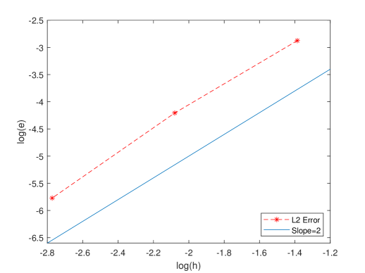
Figure 5: $\log-\log$ error.

$\kappa$	error	order
$2^{-10}$	1.1520e-04	-
$2^{-9}$	2.6185e-04	1.1846
$2^{-8}$	5.5042e-04	1.0718
$2^{-7}$	0.0011	1.0461

Table 7: Error and convergence order.

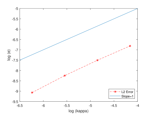
Figure 6: $\log-\log$ error.

	$E_{X_{1}}$	$E_{X_{2}}$	$V_{X_{1}}$	$V_{X_{2}}$	$V_{X_{1}X_{2}}$
PDF method	0.0956	0.0956	0.5447	0.5447	0.4047
Sample trajectories method	0.0945	0.0957	0.5499	0.5470	0.4079
Particle method	0.0937	0.0925	0.5458	0.5375	0.4032

Table 8: Expectation and covariance.

Example 3.

Consider a $2$-dimensional mean-field SDE driven by additive noise

$$dX(t)= 0.1\begin{pmatrix}-\frac{3}{2}X_{1}(t)+\frac{1}{2}X_{2}(t)+\sin(2\pi t)\\ \frac{1}{3}X_{1}(t)-\frac{4}{3}X_{2}(t)+\cos(2\pi t)\end{pmatrix}dt$$ (25)

$$+0.1\begin{pmatrix}\int_{\mathbb{R}^{2}}\frac{\sin y_{1}}{1+y_{1}^{2}}\frac{\sin y_{2}}{1+y_{2}^{2}}\mu_{t}(dy)\\ \int_{\mathbb{R}^{2}}\frac{\sin y_{1}}{1+y_{1}^{2}}\frac{\sin y_{2}}{1+y_{2}^{2}}\mu_{t}(dy)\end{pmatrix}dt+\begin{pmatrix}\frac{1}{10}\\ \frac{1}{10}\end{pmatrix}dW(t),$$

$$X(0)= (X_{0}^{1},X_{0}^{2})\overset{iid}{\sim}N(0,0.01),$$

where $W(t)$ is a $1$-dimensional Brownian motion.

The corresponding Fokker-Planck equation reads

$$\frac{\partial p}{\partial t}= -0.1\frac{\partial[(-\frac{3}{2}x_{1}(t)+\frac{1}{2}x_{2}(t)+\sin(2\pi t)+\int_{\mathbb{R}^{2}}\frac{\sin y_{1}}{1+y_{1}^{2}}\frac{\sin y_{2}}{1+y_{2}^{2}}p(t,y_{1},y_{2})dy_{1}dy_{2})p]}{\partial x_{1}}$$ (26)

$$-0.1\frac{\partial[(\frac{1}{3}x_{1}(t)-\frac{4}{3}x_{2}(t)+\cos(2\pi t)+\int_{\mathbb{R}^{2}}\frac{\sin y_{1}}{1+y_{1}^{2}}\frac{\sin y_{1}}{1+y_{1}^{2}}p(t,y_{1},y_{2})dy_{1}dy_{2})p]}{\partial x_{2}}$$

$$+\frac{1}{200}\frac{\partial^{2}p}{\partial x_{1}^{2}}+\frac{1}{100}\frac{\partial^{2}p}{\partial x_{1}\partial x_{2}}+\frac{1}{200}\frac{\partial^{2}p}{\partial x_{2}^{2}}$$

and $p_{0}(x_{1},x_{2})=\frac{1}{0.02\pi}e^{-\frac{1}{2}(\frac{x_{1}^{2}}{0.01}+\frac{x_{2}^{2}}{0.01})}$.

Notice that $\sigma=(\frac{1}{10},\frac{1}{10})^{T}$ and the rank of matrix $A=\begin{pmatrix}\frac{1}{100}&\frac{1}{100}\\ \frac{1}{100}&\frac{1}{100}\end{pmatrix}$ is of $1$. Then the assumption (A4) is violated and the Fokker-Planck equation (26) becomes degenerate. In this situation, we can not ensure the well-posedness of (26). However, our method can be used successfully to approximate (25) and (26). It is point out in [27] that the spatial convergence order is of $1$. We choose ${\mathcal{D}}=[-1,1]^{2}$ to check the corresponding temporal and spatial error estimates and convergence orders, see Tables. 10-10 and Figs. 8-8, respectively. Then, we enlarge ${\mathcal{D}}=(-4,4)^{2}$ to verify errors and convergence orders of Euler-Maruyama method (18) and expectation and covariance, cf. Table. 12.

$\kappa$	error	order
$2^{-6}$	0.0178	-
$2^{-5}$	0.0426	1.2552
$2^{-4}$	0.0946	1.1528
$2^{-3}$	0.2023	1.0960

Table 9: Error and convergence order.

$h$	error	order
$\frac{2}{48}$	0.0867	-
$\frac{2}{24}$	0.1973	1.1854
$\frac{2}{6}$	0.4114	1.0604

Table 10: Error and convergence order.

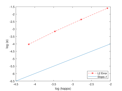
Figure 7: $\log-\log$ error.

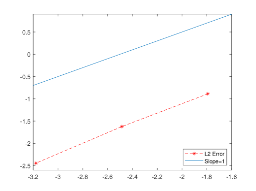
Figure 8: $\log-\log$ error.

$\kappa$	error	order
$2^{-6}$	1.2140e-04	-
$2^{-5}$	2.7785e-04	1.1984
$2^{-4}$	5.9639e-04	1.0953
$2^{-3}$	0.0013	1.0785

Table 11: Error and convergence order.

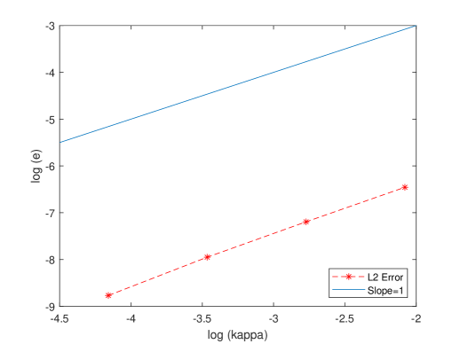
Figure 9: $\log-\log$ error.

	$E_{X_{1}}$	$E_{X_{2}}$	$V_{X_{1}}$	$V_{X_{2}}$	$V_{X_{1}X_{2}}$
PDF method	0	0	0.0165	0.0167	0.0097
Sample trajectories method	-1.1977e-04	6.0295e-04	0.0161	0.0165	0.0097
Particles method	-9.0079e-04	4.9980e-04	0.0169	0.0165	0.0098

Table 12: Expectation and covariance.

References

- \bibcommenthead
- Black and Scholes [1973] Black, F., Scholes, M.: The pricing of options and corporate liabilities. J. Polit. Econ. 81(3), 637–654 (1973) https://doi.org/10.1086/260062
- Santillán [2014] Santillán, M.: Chemical Kinetics, Stochastic Processes, and Irreversible Thermodynamics. Lecture Notes on Mathematical Modelling in the Life Sciences, p. 126 (2014). https://doi.org/10.1007/978-3-319-06689-9 . https://doi.org/10.1007/978-3-319-06689-9
- Dagan [1982] Dagan, G.: Stochastic modeling of groundwater flow by unconditional and conditional probabilities: 1. conditional simulation and the direct problem. Water Resources Research 18(4), 813–833 (1982) https://doi.org/10.1029/WR018i004p00813 https://agupubs.onlinelibrary.wiley.com/doi/pdf/10.1029/WR018i004p00813
- Baladron et al. [2012] Baladron, J., Fasoli, D., Faugeras, O.D., Touboul, J.: Mean-field description and propagation of chaos in networks of hodgkin-huxley and fitzhugh-nagumo neurons. Journal of Mathematical Neuroscience 2, 10–10 (2012)
- Patlak [1953] Patlak, C.S.: Random walk with persistence and external bias. Bulletin of Mathematical Biology 15, 311–338 (1953)
- Keller and Segel [1970] Keller, E.F., Segel, L.A.: Initiation of slime mold aggregation viewed as an instability. Journal of Theoretical Biology 26(3), 399–415 (1970) https://doi.org/10.1016/0022-5193(70)90092-5
- Banner et al. [2005] Banner, A.D., Fernholz, R., Karatzas, I.: Atlas models of equity markets. The Annals of Applied Probability 15(4) (2005) https://doi.org/10.1214/105051605000000449
- Jourdain and Reygner [2014] Jourdain, B., Reygner, J.: Capital distribution and portfolio performance in the mean-field Atlas model (2014). https://arxiv.org/abs/1312.5660
- Bossy and Talay [1997] Bossy, M., Talay, D.: A stochastic particle method for the McKean-Vlasov and the Burgers equation. Math. Comp. 66(217), 157–192 (1997) https://doi.org/10.1090/S0025-5718-97-00776-X
- dos Reis et al. [2022] Reis, G.c., Engelhardt, S., Smith, G.: Simulation of McKean-Vlasov SDEs with super-linear growth. IMA J. Numer. Anal. 42(1), 874–922 (2022) https://doi.org/10.1093/imanum/draa099
- Chen and dos Reis [2022] Chen, X., Reis, G.c.: A flexible split-step scheme for solving McKean-Vlasov stochastic differential equations. Appl. Math. Comput. 427, 127180–23 (2022) https://doi.org/10.1016/j.amc.2022.127180
- Reisinger and Stockinger [2022] Reisinger, C., Stockinger, W.: An adaptive Euler-Maruyama scheme for McKean-Vlasov SDEs with super-linear growth and application to the mean-field FitzHugh-Nagumo model. J. Comput. Appl. Math. 400, 113725–23 (2022) https://doi.org/10.1016/j.cam.2021.113725
- Belomestny and Schoenmakers [2018] Belomestny, D., Schoenmakers, J.: Projected particle methods for solving McKean-Vlasov stochastic differential equations. SIAM J. Numer. Anal. 56(6), 3169–3195 (2018) https://doi.org/10.1137/17M1111024
- Liu [2024] Liu, Y.: Particle method and quantization-based schemes for the simulation of the McKean-Vlasov equation. ESAIM Math. Model. Numer. Anal. 58(2), 571–612 (2024) https://doi.org/10.1051/m2an/2024007
- Jin et al. [2020] Jin, S., Li, L., Liu, J.-G.: Random batch methods (RBM) for interacting particle systems. J. Comput. Phys. 400, 108877–30 (2020) https://doi.org/10.1016/j.jcp.2019.108877
- Jin et al. [2021] Jin, S., Li, L., Liu, J.-G.: Convergence of the random batch method for interacting particles with disparate species and weights. SIAM J. Numer. Anal. 59(2), 746–768 (2021) https://doi.org/10.1137/20M1327641
- Jin and Li [2022] Jin, S., Li, L.: On the mean field limit of the random batch method for interacting particle systems. Sci. China Math. 65(1), 169–202 (2022) https://doi.org/10.1007/s11425-020-1810-6
- Jin and Li [[2022] ©2022] Jin, S., Li, L.: Random batch methods for classical and quantum interacting particle systems and statistical samplings. In: Active Particles. Vol. 3. Advances in Theory, Models, and Applications. Model. Simul. Sci. Eng. Technol., pp. 153–200 ([2022] ©2022)
- Evans [2013] Evans, L.C.: An Introduction to Stochastic Differential Equations, p. 151 (2013). https://doi.org/10.1090/mbk/082 . https://doi.org/10.1090/mbk/082
- Kumar et al. [2022] Kumar, C., Neelima, Reisinger, C., Stockinger, W.: Well-posedness and tamed schemes for McKean-Vlasov equations with common noise. Ann. Appl. Probab. 32(5), 3283–3330 (2022) https://doi.org/10.1214/21-aap1760
- Frank [2005] Frank, T.D.: Nonlinear Fokker-Planck Equations. Springer Series in Synergetics, p. 404 (2005). Fundamentals and applications
- Barbu and Röckner [2020] Barbu, V., Röckner, M.: From nonlinear Fokker-Planck equations to solutions of distribution dependent SDE. Ann. Probab. 48(4), 1902–1920 (2020) https://doi.org/10.1214/19-AOP1410
- LeVeque [2007] LeVeque, R.J.: Finite Difference Methods for Ordinary and Partial Differential Equations: Steady-state and Time-dependent Problems, (2007)
- Kloeden and Platen [1992] Kloeden, P.E., Platen, E.: Numerical Solution of Stochastic Differential Equations. Applications of Mathematics (New York), vol. 23, p. 632 (1992). https://doi.org/10.1007/978-3-662-12616-5 . https://doi.org/10.1007/978-3-662-12616-5
- Sauer [2013] Sauer, T.: Computational solution of stochastic differential equations. WIREs Comput. Stat. 5(5), 362–371 (2013)
- Lord et al. [2014] Lord, G.J., Powell, C.E., Shardlow, T.: An Introduction to Computational Stochastic PDEs. Cambridge Texts in Applied Mathematics, p. 503 (2014). https://doi.org/10.1017/CBO9781139017329 . https://doi.org/10.1017/CBO9781139017329
- Zhou et al. [2025] Zhou, J., Zou, Y., Konarovskyi, V., Yang, X.: Numerical approximation and dynamics of periodic solution in distribution of stochastic differential equations. Numerical Algorithms (2025)