Making Truncated Wigner for dissipative spins ‘plain easy’

Abstract

We put forward a user-friendly framework of the truncated Wigner approximation (TWA) for dissipative quantum many-body systems. Our approach is computationally affordable and it features a straightforward implementation. The leverage of the method can be ultimately traced to an intimate connection between the TWA and the semi-classical limit of the quantum Langevin equation, which we unveil by resorting to a path integral representation of the Lindbladian. Our approach allows us to explore dynamics from early to late times in a variety of models at the core of modern AMO research, including lasing, central spin models, driven arrays of Rydbergs and correlated emission in free space. Notably, our TWA outperforms the method of cumulant expansion in terms of efficiency, ease of use, and broad applicability. We therefore argue that TWA could become in the near future a primary tool for a fast and efficient first exploration of driven-dissipative many-body dynamics on consumer grade computers.

I Introduction

The dynamics of dissipative quantum many-body systems is a central topic of solid-state physics, atomic, molecular, and optical (AMO) physics, as well as quantum information science. Nearly all modern experimental platforms and quantum simulators can be modeled as interacting many-particle systems that exhibit some degree of quantum coherence, are potentially driven by external fields, and are coupled to an environment. Understanding isolated quantum many-body systems is already technically challenging, and becomes further complicated by introducing system-environment coupling. In open systems, dissipation can either suppress quantum phenomena or give rise to novel effects from the interplay of interactions and dissipation. [1, 2, 3, 4, 5, 6].

For a wide range of open quantum systems, it is possible to obtain a time-local description of dynamics that involves only the system’s degrees of freedom, without explicitly including those of the environment. In these cases, the system’s density matrix evolves according to the Lindblad master equation given by [7]

$$\derivative{t}\hat{\rho}=-i[\hat{H},\hat{\rho}]+\sum_{i}\Gamma_{ji}\,\Big{(}\hat{L}_{i}\hat{\rho}\hat{L}_{j}^{\dagger}-\frac{1}{2}\big{\{}\hat{L}_{j}^{\dagger}\hat{L}_{i},\hat{\rho}\big{\}}\Big{)},$$ (1)

where the Hamiltonian $\hat{H}$ governs coherent dynamics, while the second term captures environment-induced dissipation. Essentially, the Lindblad formalism simplifies the study of open-system dynamics by encapsulating dissipation in the jump operators $\hat{L}_{i}$, reducing the computational resources required to solve for the density matrix, compared to treating the system and environment together.

However, the numerical costs of solving Eq. (1) for generic systems still remain restrictive with current classical computers. Working with the density matrix, rather than pure states as in unitary dynamics, leads to a significantly faster growth in computational complexity with system size, which makes exact numerics impractical even for systems of a few atoms and a single photon mode. A reduced computational cost can be achieved by unraveling the Lindblad master equation (method of ‘quantum trajectories’), which bypasses the need to solve for the density matrix [8, 9]. Nevertheless, without resorting to approximations, about a dozen degrees of freedom remains the upper limit to the exact numerical solutions of Eq. (1).

Progress in scientific discovery is fueled by flexible and speedy approaches to reliably test starting hypotheses, which can then serve as a solid starting point for the development of more sophisticated and resource-intensive methods. In the view of the authors’ of this work, such approach should meet three key criteria. (i) It is computationally affordable, allowing the study of dynamics in the many-body limit and for sufficiently long times using the available classical computers (possibly, even standard consumer laptops). (ii) It captures quantum effects to a sufficient extent. Notably, this requirement is relatively modest for most driven-open many-body AMO (or solid state) systems, as they typically exhibit limited quantum fluctuations due to major role played by dissipation. Many-body phenomena driven by strong quantum effects are rare in these platforms and stand out precisely due to their pronounced quantum character (see for instance [10, 11] for spin liquids in light-matter interfaces). (iii) The method should feature a straightforward implementation, requiring no fine-tuning for each specific problem, and, ideally, be accessible to first-time users with minimal effort.

Our work aims at putting forward a semi-classical method for solving driven-dissipative quantum many body systems, satisfying all the three above mentioned criteria. To better appreciate the relevance of our framework, we will first shortly summarize the state of the art in computational methods for solving driven open quantum systems.

An accessible method, which is widely used as the first attempt to attack new problems, is the mean-field (MF) approximation. By neglecting all quantum corrections, MF describes the system through classical equations of motion for the expectation values of physical observables. This approach is particularly effective for all-to-all interacting models (such as Dicke, Tavis-Cummings, or Lipkin-Meshkov-Glick), where quantum fluctuations are suppressed as the system size increases [12, 13, 14, 15, 16, 17]. MF does, therefore, addresses the criteria (i) and (iii) above, while failing on (ii). Beyond the collective limit, MF is well-known to give inaccurate predictions, and its accuracy can be improved by accounting for correlations between observables, captured by the connected parts of multi-point correlation functions. This approach leads to an infinite hierarchy of coupled differential equations for correlation functions. Truncating this hierarchy at a finite level, by neglecting higher-order connected correlation functions and obtaining a closed set of equations, results in the method of cumulant expansion (CE) [18, 19, 20, 21, 22]. Usually, CE provides significant improvement over MF results, sometimes even matching the exact solution [18]. However, when truncation at a given order fails to produce satisfactory results, or suffers from numerical instabilities [20], or when higher-order correlations need to be explored, one must retain additional equations in the hierarchy or selectively exclude certain correlation functions based on heuristic choices. In some cases, the accuracy of CE decreases at higher orders of the expansion [23, 24]. These issues introduce an arbitrary element into the approximation, compromising its reliability and, essentially, requiring prior knowledge of the solution to the problem. Therefore, while improving on the criterion (ii) by introducing quantum fluctuations on top of mean-field, it fails criterion (iii), and to some extent (i), as we will also further discuss in the body of the paper.

More advanced techniques such as tensor networks  [25, 26, 27, 28, 29, 30], variational principles [31, 32, 33] and quantum kinetic equations based on diagrammatics [34, 35, 5, 36, 37, 38, 39, 40, 41, 42, 43, 44], require substantial expertise and time investment. While the former is of particular great efficacy in low dimensions, the latter two require strong physical intuition and solid theoretical background on the problem at hand. These methods represent primary examples of those sophisticated and resource-intensive approaches, that should be employed once it becomes clear that solving the physical problem under scrutiny requires the inclusion of strong correlations on long time scales and large system sizes. As methods suited for first exploratory studies, they would certainly fail criteria (i) and (iii).

For isolated systems, the truncated Wigner approximation (TWA) is a method that satisfies all the three criteria outlined above. Broadly speaking, it approximates quantum dynamics using classical statistical mechanics, where quantum uncertainty is mapped onto a classical probability distribution through the Wigner transformation of system’s density matrix [45], and expectation values of observables are approximated by their statistical averages over an ensemble of classical trajectories. In the absence of external dissipation, each trajectory is initialized by sampling from the corresponding probability distribution and evolves according to classical equations of motion. While these equations resemble those of MF, the statistical sampling of initial conditions accounts for leading-order quantum fluctuations (criterion (ii)). TWA has been notably successful in describing the dynamics of isolated bosonic [46, 47] and spin systems [48], and has been promisingly extended to fermions [49]. The combination of a MF logic with a straightforward stochastic sampling makes TWA computationally affordable even for large system sizes and long times (i), as well as easy to implement (iii).

However, extending TWA to open quantum systems has proven more challenging, with success largely limited to some of the simplest dissipation channels. In particular, a universal framework for dissipative spin systems—widely used to model ensembles of two-level atoms in AMO physics—has remained elusive to this day. In general, dissipation arises from the interplay between deterministic and stochastic elements where, analogous to the classical Langevin equation, the deterministic component appears as damping, while the stochastic component manifests as noise [35, 50]. The key challenge in dissipative TWA is to properly incorporate both elements into the equations of motion, which has led to various issues in existing implementations. These issues include spin-length shrinkage for individual trajectories, which erases the relevant physics beyond short times [51, 52, 53, 54], and restricted applicability to collective (i.e., very large) spin sizes [55]. There are approaches that overcome the mentioned issues, but have limited flexibility and scalability for application to new problems due to the complexity of their formulation [56, 57, 58], failing criterion (iii).

In this work, we present a state-of-the-art formulation of TWA for Lindblad dynamics that addresses all major issues discussed above. Our approach is general and applies to arbitrary degrees of freedom and dissipation channels. Despite its flexibility, the method remains highly intuitive, requiring only a basic understanding of stochastic differential equations. Due to its systematic derivation, it provides a controlled and conserving approximation, avoiding issues such as artificial spin shrinkage [55]. We develop the formalism using the Keldysh path-integral representation of quantum dynamics, and by expanding the action to second order in quantum fluctuations [35]. Our work is inspired by the approach of Refs. [47, 45], which derived TWA for closed bosonic systems by truncating the Keldysh action at first order in quantum fluctuations. While the derivation relies on field theoretical arguments, the resulting framework can be applied without prior knowledge of field theory, by resorting to a simple recipe outlined in Sec. II.1 (see also Fig. 1). Notably, the equations of motion admit an intuitive interpretation as a semiclassical limit of the quantum Langevin equation (QLE) for dissipative operator dynamics [59]. By applying our method to various examples and comparing the results to exact solutions, we demonstrate its overall advantages over other approaches. In particular, our method surpasses CE in all of the comparisons. Thus, we believe that our framework could replace CE as the first-choice tool for studying dissipative quantum many-body systems.

We begin in Sec. II by introducing a straightforward protocol for applying our dissipative TWA to general problems, while postponing its formal field-theoretic derivation to Appendix A. In Sec. III, we specialize our approach to dissipative spin systems before applying it to a series of increasingly complex examples. These include a single driven spin, the Tavis-Cummings model for lasing, the central spin model, a driven Rydberg chain, and finally, the dynamics of a sub-wavelength atomic chain with correlated emission. We conclude in Sec. IV by giving an overview of the work, and discussing potential applications of the method and exploring its possible extensions.

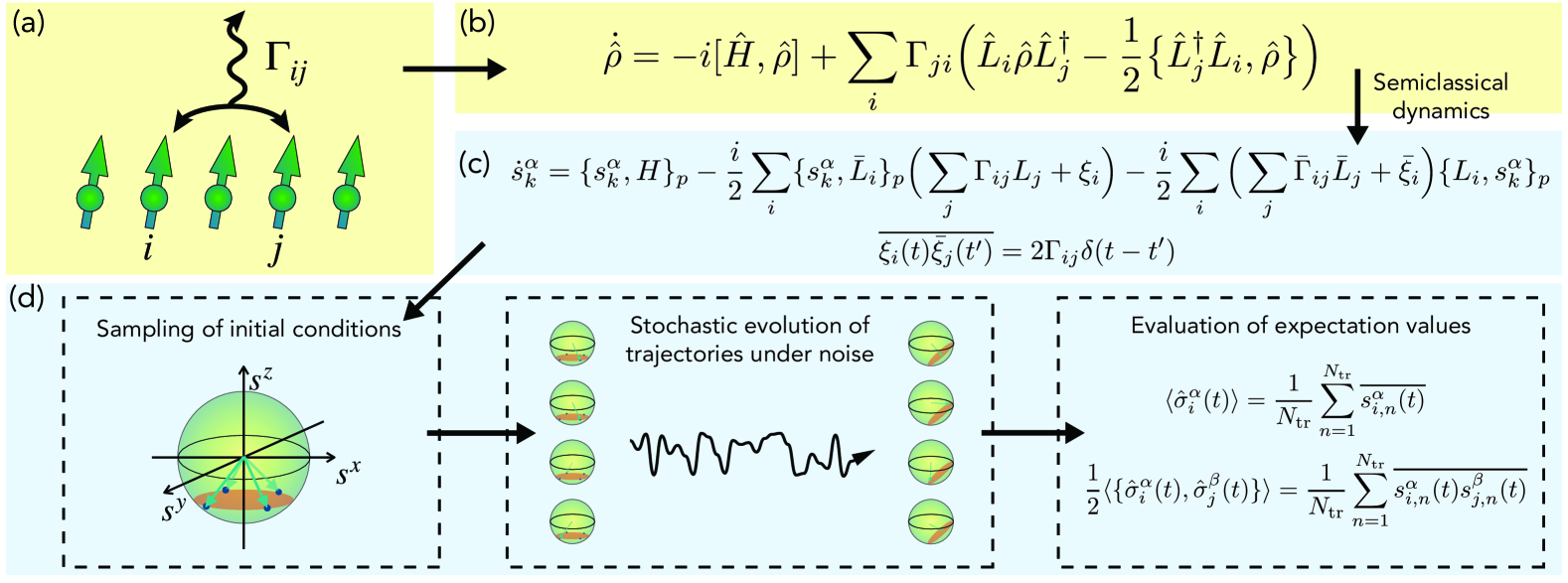
Figure 1: Schematic overview of the method for dissipative spins. (a) A system of spins subjected to dissipation. (b) The exact quantum dynamics are governed by the Lindblad master equation. (c) The semiclassical approximation replaces quantum spins with classical variables, evolving according to stochastic differential equations. (d) Classical spin variables are initialized by sampling from a distribution function (shown here with discrete sampling) and then evolved under the classical equations with added noise. Quantum expectation values are approximated by averaging over multiple trajectories and noise realizations.

II Method

In Section II.1 below, we focus on the main result of this work, by expressing the method in terms of an effective classical Hamiltonian that encapsulates all relevant aspects of the approximation. The field-theoretic derivation is presented in detail in Appendix A, and does not rely on a Fokker-Planck equation for the classical distribution function. Instead, it operates directly with classical trajectories and their averages. In Sec. II.2, we demonstrate that the equations of motion closely resemble QLE for dissipative operator dynamics, with quantum commutators replaced by classical Poisson brackets.

II.1 General protocol

We consider the dynamics of Lindblad systems as given by the general expression in Eq. (1). Taking $\hat{\psi}_{\alpha}$ as the set of basic operator degrees of freedom in the system, e.g. spins or boson creation and annihilation operators, the semiclassical dynamics can be obtained using the following prescription (see Appendix A for a derivation):

1. Replace quantum operators $\hat{\psi}_{\alpha}$ with the classical dynamical variables $\psi_{\alpha}$ and consequently, obtain the classical Hamiltonian ($\hat{H}\to H$) and jump operators ($\hat{L}_{i}\to L_{i}$).

2. Construct the following effective classical Hamiltonian which captures dissipation by coupling the system’s jump variables to a set of self-consistent fields:

   $$\tilde{H}=H-i\sum_{i}\big{(}\bar{L}_{i}\Phi_{i}-\bar{\Phi}_{i}L_{i}\big{)},$$ (2)

   where the bar stands for complex conjugation. This yields the equations of motion for $\psi_{\alpha}$ from

   $$\derivative{t}\psi_{\alpha}=\{\psi_{\alpha},\tilde{H}\}_{p},$$ (3)

   where the Poisson bracket can be obtained mostly easily from the quantum commutators using the Dirac correspondence [60]

   $$\{A,B\}_{p}\longleftrightarrow-i[\hat{A},\hat{B}].$$ (4)

3. Substitute the following formula for the variables $\Phi_{i}$ in the equations of motion

   $$\Phi_{i}=\frac{1}{2}\sum_{j}\Gamma_{ij}L_{j}+\frac{1}{2}\xi_{i},$$ (5)

   where $\xi_{i}$ is a Gaussian noise defined by

   $$\overline{\xi_{i}(t)}=0,\quad\overline{\xi_{i}(t)\bar{\xi}_{j}(t^{\prime})}=2\Gamma_{ij}\delta(t-t^{\prime}),$$ (6)

   where bars here indicate noise averages (not to be confused with the same notation used for complex conjugation in Eq. (2)).

   We emphasize that the expression for $\Phi_{i}$ has to be substituted only after obtaining the equations of motion.

4. The outcome of the above steps is

   $$\derivative{t}\psi_{\alpha}=\{\psi_{\alpha},H\}_{p}-\frac{i}{2}\sum_{i}\{\psi_{\alpha},\bar{L}_{i}\}_{p}\Big{(}\sum_{j}\Gamma_{ij}L_{j}+\xi_{i}\Big{)}\\ -\frac{i}{2}\sum_{i}\Big{(}\sum_{j}\bar{\Gamma}_{ij}\bar{L}_{j}+\bar{\xi}_{i}\Big{)}\{L_{i},\psi_{\alpha}\}_{p},$$ (7)

   which is the semiclassical equation of motion, and the central result of this work.

5. Sample initial conditions for classical variables according to the initial probability distribution function, to account for the quantum uncertainty in the initial state. For each initial condition, obtain a trajectory by evaluating stochastic dynamics according to Eq. (7).

6. Obtain the expectation values of observables by taking their average over different trajectories and noise realizations.

The initial distribution function can be obtained by taking the Wigner transformation of initial density matrix, as thoroughly discussed in Ref. [45]. For spin-$1/2$ degrees of freedom, one can also use a discrete sampling of the initial state, which can yield improved results [61, 48]. We will discuss the discrete sampling later in more details, when we address spin systems as a special case in Sec. III.1.

II.2 Connection to the quantum Langevin equation

We emphasize that the resulting protocol above is not merely an outcome of the field theory ‘black box’. Notably, using the Dirac correspondence in Eq. (4), we can interpret Eq. (7) as the semiclassical limit of QLE

$$\derivative{t}\hat{\psi}_{\alpha}=i[\hat{H},\hat{\psi}_{\alpha}]-\frac{1}{2}\sum_{i}\big{[}\hat{\psi}_{\alpha},\hat{L}_{i}^{\dagger}\big{]}\Big{(}\sum_{j}\Gamma_{ij}\hat{L}_{j}+\hat{\xi}_{i}\Big{)}\\ -\frac{1}{2}\sum_{i}\Big{(}\sum_{j}\bar{\Gamma}_{ij}\hat{L}_{j}^{\dagger}+\hat{\xi}_{i}^{\dagger}\Big{)}\big{[}\hat{L}_{i},\hat{\psi}_{\alpha}\big{]},$$ (8)

which describes the dynamics of quantum mechanical operators in the presence of dissipation, and is an alternative, but equivalent, representation of Lindblad master equation (Eq. (1)), with quantum noise $\langle\hat{\xi}_{i}(t)\hat{\xi}_{j}^{\dagger}(t^{\prime})\rangle=2\Gamma_{ij}\delta(t-t^{\prime})$ [59, 62]. We recall that at the level of Eq. (8) the noise, $\hat{\xi}_{i}(t)$, is an operator since it encapsulates the interaction between the quantum degrees of freedom of the system and of the environment (also operators in a microscopic description of system-bath coupling).

A crucial point to remember about the classical equation Eq. (7) is that all variables are numbers, meaning they commute and should no longer be treated as operators. If, instead, we start with QLE (8), simplify the right-hand side using operator commutation relations, and take the classical limit afterwards, the resulting equations can be inconsistent with the semi-classical approximation [63]. We will discuss this issue in more details later in Sec. III for dissipative spins.

III Results for dissipative spins

In this section, we explore practical applications of our dissipative TWA to spin models. We begin in Sec. II.1 by specializing the protocol presented in Sec. II.1 to spins, together with remarks on the sampling of initial states. As a first example, Sec. III.2 examines a coherently driven spin subject to decay. We then analyze models with long-range interactions, including the Tavis-Cummings and central spin models, in Secs. III.3 and III.4, respectively. In Sec. III.5, we shift focus to short-range interactions, solving the dynamics of a driven Rydberg chain. Finally, Sec. III.6 extends our approach beyond individual dissipation by considering an atomic chain with correlated emission.

III.1 Protocol for spins

Below, we mainly restate the rules of Sec. II.1 for spin degrees of freedom, which are also illustrated in Fig. 1 for clarity. We will also briefly discuss the discrete sampling of initial conditions.

1. Replace spin operators $\hat{\bm{\sigma}}_{k}=(\sigma^{x}_{k},\sigma^{y}_{k},\sigma^{z}_{k})$ with the classical variables $\bm{s}_{k}=({s}_{k}^{x},{s}_{k}^{y},{s}_{k}^{z})$ and substitute them in the Hamiltonian and jump operators.

2. The equation of motion for $s^{\alpha}_{k}$ follows from

   $$\derivative{t}s_{k}^{\alpha}=\{{s}_{k}^{\alpha},\tilde{H}\}_{p},$$ (9)

   with the effective classical Hamiltonian

   $$\tilde{H}=H-i\sum_{i}\big{(}\bar{L}_{i}\Phi_{i}-\bar{\Phi}_{i}L_{i}\big{)}.$$ (10)

   The Poisson’s bracket of spin variables with another variable $O$ can be expressed as

   $$\{{s}_{k}^{\alpha},O\}_{p}=2\sum_{\beta,\gamma}\epsilon_{\alpha\beta\gamma}\frac{\partial O}{\partial s_{k}^{\beta}}s_{k}^{\gamma},$$ (11)

   where $\epsilon_{\alpha\beta\gamma}$ is the totally anti-symmetric tensor with $\epsilon_{xyz}=+1$.

3. Substitute for $\Phi_{i}$ using Eqs. (5) and (6) to get the classical Langevin equation for spins

   $$\derivative{t}s_{k}^{\alpha}=\{s_{k}^{\alpha},H\}_{p}-\frac{i}{2}\sum_{i}\{s_{k}^{\alpha},\bar{L}_{i}\}_{p}\Big{(}\sum_{j}\Gamma_{ij}L_{j}+\xi_{i}\Big{)}\\ -\frac{i}{2}\sum_{i}\Big{(}\sum_{j}\bar{\Gamma}_{ij}\bar{L}_{j}+\bar{\xi}_{i}\Big{)}\{L_{i},s_{k}^{\alpha}\}_{p},$$ (12)

   The final form of this equation is provided in Table 1 for some of the common dissipation channels. Since the equations of motion are obtained from an effective Hamiltonian, which is a function of spin variables, we have

   $$\derivative{t}|\bm{s}_{k}|^{2}=4\sum_{\alpha\beta\gamma}\epsilon_{\alpha\beta\gamma}s_{k}^{\alpha}\frac{\partial\tilde{H}}{\partial s^{\beta}_{k}}s^{\gamma}_{k}=0,$$ (13)

   due to the anti-symmetry property $\epsilon_{\alpha\beta\gamma}=-\epsilon_{\gamma\beta\alpha}$. Therefore, regardless of dissipation profile, the length of spins is always conserved for each trajectory, which is an essential condition for the consistency of TWA.

4. In the next step, we sample initial conditions for $\bm{s}_{k,n}$ with $n=1,\dots,N_{\mathrm{tr}}$ to account for quantum uncertainty in the initial state, where $N_{\mathrm{tr}}$ is the number of sampled trajectories.

5. For each trajectory, evaluate stochastic dynamics according to Eq. (7).

6. Expectation values, and symmetric two-point functions are obtained from averaging over trajectories and noise realizations:

   $$\langle\hat{\sigma}_{k}^{\alpha}(t)\rangle =\frac{1}{N_{\mathrm{tr}}}\sum_{n=1}^{N_{\mathrm{tr}}}\overline{s_{k,n}^{\alpha}(t)}$$ (14)

   $$\frac{1}{2}\langle\{\hat{\sigma}_{k}^{\alpha}(t),\hat{\sigma}_{l}^{\beta}(t)\}\rangle =\frac{1}{N_{\mathrm{tr}}}\sum_{n=1}^{N_{\mathrm{tr}}}\overline{s_{l,n}^{\alpha}(t)s_{k,n}^{\beta}(t)},$$

   where overlines represent averaging over the noise, and $\{A,B\}=AB+BA$ is the anti-commutator.

$\hat{L}_{i}$	Equations of motion
$\sqrt{\gamma_{\downarrow}}\,\hat{\sigma}^{-}$	$\begin{aligned} &\mathrm{d}s^{x}/\mathrm{d}t=\gamma_{\downarrow}s^{x}s^{z}/2+\xi_{\downarrow}^{x}s^{z}\\ &\mathrm{d}s^{y}/\mathrm{d}t=\gamma_{\downarrow}s^{y}s^{z}/2+\xi_{\downarrow}^{y}s^{z}\\ &\mathrm{d}s^{z}/\mathrm{d}t=-\gamma_{\downarrow}\,(s^{x}s^{x}+s^{y}s^{y})/2-(\xi_{\downarrow}^{x}s^{x}+\xi_{\downarrow}^{y}s^{y})\\ &\overline{\xi_{\downarrow}^{\alpha}(t)\,\xi_{\downarrow}^{\beta}(t^{\prime})}=\gamma_{\downarrow}\,\delta_{\alpha\beta}\,\delta(t-t^{\prime})\end{aligned}$
$\sqrt{\gamma_{\uparrow}}\,\hat{\sigma}^{+}$	$\begin{aligned} &\mathrm{d}s^{x}/\mathrm{d}t=-\gamma_{\uparrow}s^{x}s^{z}/2-\xi_{\uparrow}^{x}s^{z}\\ &\mathrm{d}s^{y}/\mathrm{d}t=-\gamma_{\uparrow}s^{y}s^{z}/2+\xi_{\uparrow}^{y}s^{z}\\ &\mathrm{d}s^{z}/\mathrm{d}t=\gamma_{\uparrow}\,(s^{x}s^{x}+s^{y}s^{y})/2+(\xi_{\uparrow}^{x}s^{x}-\xi_{\uparrow}^{y}s^{y})\\ &\overline{\xi_{\uparrow}^{\alpha}(t)\,\xi_{\uparrow}^{\beta}(t^{\prime})}=\gamma_{\uparrow}\,\delta_{\alpha\beta}\,\delta(t-t^{\prime})\end{aligned}$
$\sqrt{\kappa}\,\hat{\sigma}^{z}$	$\begin{aligned} &\mathrm{d}s^{x}/\mathrm{d}t=+2\,\eta s^{y}\\ &\mathrm{d}s^{y}/\mathrm{d}t=-2\,\eta s^{x}\\ &\mathrm{d}s^{z}/\mathrm{d}t=0\\ &\overline{\eta(t)\,\eta(t^{\prime})}=\kappa\,\delta(t-t^{\prime})\end{aligned}$

Table 1: Classical equations of motion for incoherent spin loss, spin pump and dephasing. Note that we have absorbed the rates into the jump operators such that $\Gamma_{ij}=\delta_{ij}$ in Eq. (1). The real-valued noises originate from the real and imaginary parts of the complex noises introduced in Eq. (12).

In practice, the sampling of initial state and the noise can be performed together, i. e., we can write

$$\frac{1}{N_{\mathrm{tr}}}\sum_{n=1}^{N_{\mathrm{tr}}}\overline{s_{k,n}^{\alpha}(t)}=\frac{1}{N_{\mathrm{tot}}}\sum_{n^{\prime}=1}^{N_{\mathrm{tot}}}s_{k,n^{\prime}}^{\alpha}(t),$$ (15)

where $N_{\mathrm{tot}}=N_{\mathrm{tr}}\times N_{\mathrm{noise}}$ and $N_{\mathrm{noise}}$ is the number of noise realizations. In the following sections, we will use a discrete sampling of initial conditions for spin-1/2 degrees of freedom, also known as discrete TWA (DTWA) [48, 61, 64]. For instance, for the initial state with $\sigma^{z}_{k}\ket{\downarrow}=-\ket{\downarrow}$, we sample the classical initial states according to the following discrete distribution

$$W_{0}(s^{x}_{k},s^{y}_{k},s^{z}_{k})=\begin{cases}0&\quad(s^{x}_{k},s^{y}_{k},s^{z}_{k})=(\pm 1,\pm 1,+1),\\ 1/4&\quad(s^{x}_{k},s^{y}_{k},s^{z}_{k})=(\pm 1,\pm 1,-1),\end{cases}$$ (16)

which has been shown to yield improved results in certain cases, in comparison to continuous sampling of initial spin states [48]. We then solve Eq. (12) using an implicit numerical integration scheme and the Stratonovich regularization of stochastic dynamics [59, 35].

We emphasize that our approach does not rely on any specific representation of spin operators, such as Schwinger bosons or spin coherent states. Likewise, our derivation in Appendix A is representation-independent, following directly from general field-theoretic arguments.

III.2 Driven spin

As a first example, we consider a coherently driven single spin. The exact solvability of this problem allows us to evaluate the accuracy of our semiclassical approximation and determine its range of applicability. The dynamics of the spin are governed by the following Hamiltonian

$$\hat{H}=\Omega\,\hat{\sigma}^{x},$$ (17)

with the Rabi frequency $\Omega$, together with incoherent loss ($\hat{L}^{\downarrow}=\hat{\sigma}^{-}$) with the rate $\gamma_{\downarrow}$. Using Eq. (12), we obtain the following equations of motion for classical spin variables $(s^{x},s^{y},s^{z})$

$$\derivative{t}s^{x} =+\frac{\gamma_{\downarrow}}{2}s^{x}s^{z}+\xi_{\downarrow}^{x}s^{z},$$ (18)

$$\derivative{t}s^{y} =-2\,\Omega\,s^{z}+\frac{\gamma_{\downarrow}}{2}s^{y}s^{z}+\xi_{\downarrow}^{y}s^{z},$$ (19)

$$\derivative{t}s^{z} =+2\,\Omega\,s^{y}-\frac{\gamma_{\downarrow}}{2}\Big{(}(s^{x})^{2}+(s^{y})^{2}\Big{)}-\xi_{\downarrow}^{x}s^{x}-\xi_{\downarrow}^{y}s^{y},$$ (20)

where the noise fields satisfy

$$\overline{\xi_{\downarrow}^{\alpha}(t)\,\xi_{\downarrow}^{\beta}(t^{\prime})}=\gamma_{\downarrow}\delta_{\alpha\beta}\delta(t-t^{\prime}).$$ (21)

Fig. 2 compares the exact solution with semiclassical results obtained from Eqs. (18)-(20) for different values of $\gamma_{\downarrow}$. We observe that TWA captures exact dynamics for weak to moderate losses ($\gamma_{\downarrow}\lesssim\Omega$), while it progressively deviates from the correct answer for larger decay rates. In the extreme limit $\Omega\to 0$, TWA captures early-time dynamics correctly, while deviating from the correct steady state at later times. The accuracy of the method also improves in the presence of incoherent pumping ($\hat{L}^{\uparrow}=\hat{\sigma}^{+}$), with the highest accuracy achieved when $\gamma_{\uparrow}=\gamma_{\downarrow}$.

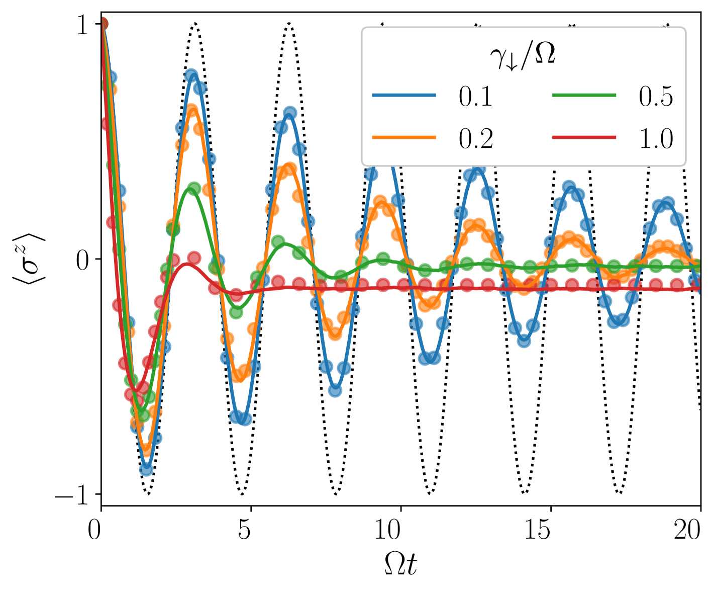
Figure 2: Evolution of a single spin under coherent driving and spontaneous decay. TWA (solid lines) shows strong agreement with the exact solution (circles) for weak to moderate loss rates ($\gamma_{\downarrow}\lesssim\Omega$). For $\gamma_{\downarrow}\gtrsim\Omega$, quantum fluctuations grow beyond the reach of our semiclassical approximation and cause deviations from the exact solution. The dotted line corresponds to $\gamma_{\downarrow}/\Omega=0.1$ without including noise. The results have been obtained by averaging over $O(10^{5})$ trajectories.

As we showed earlier in Eq. (13), our approach conserves the size of spins for each trajectory, since it takes the ‘proper’ classical limit of QLE (Eq. (8)). Therefore, it is instructive to consider also the ‘improper’ classical limit of QLE for this problem, in order to juxtapose these two classical approximations. First, we substitute the spin and jump operators in Eq. (7), without simplifying the resulting equations:

$$\derivative{t}\hat{\sigma}^{x} =+\frac{1}{2}\hat{\sigma}^{z}\big{(}\gamma_{\downarrow}\hat{\sigma}^{-}+\hat{\xi}_{\downarrow}\big{)}+\frac{1}{2}\big{(}\gamma_{\downarrow}\hat{\sigma}^{+}+\hat{\xi}_{\downarrow}^{\dagger}\big{)}\hat{\sigma}^{z},$$ (22)

$$\derivative{t}\hat{\sigma}^{y} =-2\,\Omega\,\hat{\sigma}^{z}+\frac{i}{2}\hat{\sigma}^{z}\big{(}\gamma_{\downarrow}\hat{\sigma}^{-}+\hat{\xi}_{\downarrow}\big{)}-\frac{i}{2}\big{(}\gamma_{\downarrow}\hat{\sigma}^{+}+\hat{\xi}_{\downarrow}^{\dagger}\big{)}\hat{\sigma}^{z},$$ (23)

$$\derivative{t}\hat{\sigma}^{z} =+2\,\Omega\,\hat{\sigma}^{y}-\frac{1}{2}\hat{\sigma}^{+}\big{(}\gamma_{\downarrow}\hat{\sigma}^{-}+\hat{\xi}_{\downarrow}\big{)}-\frac{1}{2}\big{(}\gamma_{\downarrow}\hat{\sigma}^{+}+\hat{\xi}_{\downarrow}^{\dagger}\big{)}\hat{\sigma}^{-}.$$ (24)

If we now take the classical limits of these equations, we immediately get Eqs. (18)-(20), with $\xi_{\downarrow}^{x}$ and $\xi_{\downarrow}^{y}$ given by the real and imaginary parts of the complex-valued noise $\xi_{\downarrow}$. However, if we proceed to simplify these equations by using the spin commutation relations for the non-noisy terms and then take the classical limit, we obtain

$$\derivative{t}s^{x} =-\frac{\gamma_{\downarrow}}{2}s^{x}+\xi_{\downarrow}^{x}s^{z},$$ (25)

$$\derivative{t}s^{y} =-2\,\Omega\,s^{z}-\frac{\gamma_{\downarrow}}{2}s^{y}+\xi_{\downarrow}^{y}s^{z},$$ (26)

$$\derivative{t}s^{z} =+2\,\Omega\,s^{y}-\frac{\gamma_{\downarrow}}{2}(1+s^{z})-\xi_{\downarrow}^{x}s^{x}-\xi_{\downarrow}^{y}s^{y},$$ (27)

which reduce the length of spin over time, leading to a trivial limit at long times. To resolve this issue, previous works [63] introduced an ad-hoc modification to the noise terms, such that the spin-shrinkage rate becomes small. However, the exact equations for $\langle\hat{\bm{\sigma}}\rangle$ are identical to Eqs. (25)-(27) without the noise terms. This suggests that the noise is an artifact introduced solely to make the semiclassical approximation feasible by artificially generating statistical uncertainty.

In contrast, noise plays a crucial role in our approach and naturally arises from expanding the dynamics order by order in quantum fluctuations. At the leading-order, the quantum contribution is captured by the statistical sampling of the initial state, while noise emerges at the next-to-leading-order. Consequently, the effect of noise becomes less significant when deterministic contributions dominate the dynamics. This occurs, for instance, when the system is strongly driven, ($\Omega\gtrsim\gamma_{\downarrow}$), as shown earlier, or in the collective-spin limit where $S$ is large, while rescaling $\gamma_{\downarrow}$ such that the limit $S\to\infty$ remains well-defined. In the latter case, mean-field equations become exact, and noise is negligible [7]. Conversely, when quantum effects fully dominate, such as for $S=1/2$ and $\Omega\ll\gamma_{\downarrow}$, higher-order corrections beyond noise must be included for accurate results. In the intermediate regime, where $S$ is small but $\Omega\gtrsim\gamma_{\downarrow}$, incorporating noise while discarding higher order effects is sufficient, whereas neglecting the noise leads to significant errors. This has been explicitly demonstrated in Fig. 2, where solving the equations without noise results in a dramatic deviation from the correct dynamics, even for weak dissipation.

We note that while some alternative approaches to TWA can accurately capture single-spin decay across all decay rates [56, 57], they are restricted to $S=1/2$. In contrast, our method is general and seamlessly interpolates between the two extreme limits of $S=1/2$ and $S\to\infty$ within a unified framework. Furthermore, as demonstrated below, for the practical purposes of solving many-body dynamics, both our approach and those in Refs. [56, 57] achieve similar accuracy, while ours remains conceptually and computationally simpler.

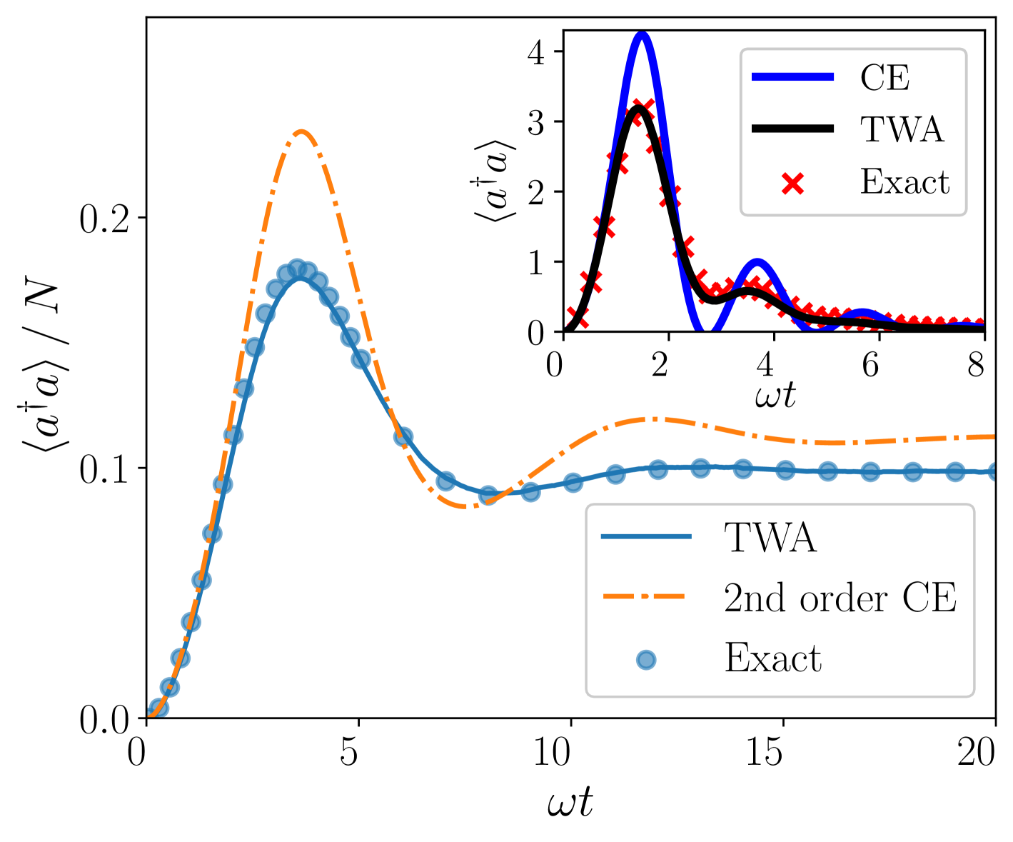
Figure 3: The evolution of the normalized photon population in the dissipative Tavis-Cummings model with $N=15$, starting with the photonic vacuum with fully inverted atoms. TWA demonstrates excellent agreement with the exact solution, whereas the second-order CE becomes inaccurate beyond short times. The parameters used are $\omega=\epsilon=\kappa$, $g/\omega=9/10$, $\gamma_{\downarrow}/\omega=1/8$, and $\gamma_{\uparrow}/\omega=3/8$. Inset: Dynamics of photon population without incoherent pump ($\gamma_{\uparrow}=0$) for $N=12$ spins, showing good agreement between TWA and the exact result. The other parameters are $\omega=\kappa=2\epsilon$, $g/\omega\approx 1.7$, and $\gamma_{\downarrow}/\omega=0.25$. TWA results are obtained from $O(10^{5})$ trajectories.

III.3 Tavis-Cummings model

The first model we analyze is in the class of all-to-all interacting systems. As mentioned in the introduction, these models are particularly instrumental in systematically studying corrections on top of mean field dynamics, since they are usually equipped with a ‘large N’ parameter [17, 16].

The Tavis-Cummings (TC) model is a prototypical model for lasing [7, 65] which finds applications in modern AMO research, in particular, to study ultra-narrow linewidth lasing in a bad cavity [66, 67, 68, 69, 70] and dynamical phase transitions between non-radiative, lasing and superradiant lasing regimes [71, 18]. TC consists of a single bosonic mode, representing photons, coupled to an ensemble of spin-$1/2$ degrees of freedom, modeling two-level atoms confined within an optical cavity. Its relevance in our narrative is as a first step in comparing the efficiency of TWA and CE in capturing the dynamics and steady states of driven-open systems.

The TC Hamiltonian reads

$$\hat{H}=\omega\,\hat{a}^{\dagger}\hat{a}+\frac{\epsilon}{2}\sum_{i=1}^{N}\hat{\sigma}^{z}_{i}+\frac{g}{\sqrt{N}}\sum_{i=1}^{N}\Big{(}\hat{a}^{\dagger}\hat{\sigma}^{-}_{i}+\hat{a}\hat{\sigma}^{+}_{i}\Big{)}.$$ (28)

Incoherent processes include photon loss ($\hat{L}^{\kappa}=\hat{a}$), atomic loss ($\hat{L}^{\downarrow}_{i}=\hat{\sigma}^{-}_{i}$), and atomic pumping ($\hat{L}^{\uparrow}_{i}=\hat{\sigma}^{+}_{i}$), with respective rates $\kappa$, $\gamma_{\downarrow}$, and $\gamma_{\uparrow}$. In the absence of dissipation, the TC model exhibits a $U(1)$ symmetry, defined by the transformation $(\hat{a},\hat{\sigma}^{-}_{i})\to(e^{i\phi}\hat{a},e^{i\phi}\hat{\sigma}^{-}_{i})$, which ensures the conservation of the total number of excitations, $\hat{n}_{\mathrm{tot}}=\hat{a}^{\dagger}\hat{a}+\sum_{i}\hat{\sigma}^{z}_{i}/2$. Additionally, the model possesses permutation symmetry under spin exchange. These symmetries render the model integrable, allowing its solution by separately analyzing subspaces of the Hilbert space with fixed excitation number and total angular momentum.

However, dissipation typically breaks these symmetries. Photon loss only breaks $U(1)$ symmetry while preserving permutation symmetry, still making exact solutions feasible for sufficiently large system sizes. In contrast, individual atomic decay breaks both symmetries, significantly complicating the solution. Although weak permutation symmetry can still be exploited to reduce computational costs for steady-state calculations [13, 23], exact time evolution remains accessible only for small systems. Common approximation methods, such as MF theory and cumulant expansion (CE), often yield inconsistent results, which also depend on the order of CE [23]. In some cases, these approximations approach the correct result in the $N\to\infty$ limit, but they typically exhibit slow convergence. That is, even for large but finite system sizes, deviations from exact solutions persist over a broad parameter range.

To solve the problem with TWA, we substitute photon and spin variables into Eq. (7) to get the following equations of motion

$$\derivative{t}a =-i\omega a-\frac{ig}{\sqrt{N}}\sum_{i}s^{-}_{i}-\frac{\kappa}{2}a-\frac{1}{2}\xi_{\kappa},$$ (29)

$$\derivative{t}s^{x}_{i} =-\epsilon s^{y}_{i}-\frac{2g}{\sqrt{N}}s^{z}_{i}\,\mathrm{Im}\,a+\frac{\gamma_{\downarrow}-\gamma_{\uparrow}}{2}s^{x}_{i}s^{z}_{i}+\big{(}\xi_{\downarrow,i}^{x}-\xi_{\uparrow,i}^{x}\big{)}s^{z}_{i},$$ (30)

$$\derivative{t}s^{y}_{i} =+\epsilon s^{x}_{i}-\frac{2g}{\sqrt{N}}s^{z}_{i}\,\mathrm{Re}\,a+\frac{\gamma_{\downarrow}-\gamma_{\uparrow}}{2}s^{y}_{i}s^{z}_{i}+\big{(}\xi_{\downarrow,i}^{y}+\xi_{\uparrow,i}^{y}\big{)}s^{z}_{i},$$ (31)

$$\derivative{t}s^{z}_{i} =+\frac{4g}{\sqrt{N}}\,\mathrm{Im}\,\big{(}a\,s^{+}_{i}\big{)}-\frac{\gamma_{\downarrow}-\gamma_{\uparrow}}{2}\Big{(}(s^{x}_{i})^{2}+(s^{y}_{i})^{2}\Big{)}$$

$$\qquad\qquad\qquad+\big{(}\xi^{x}_{\uparrow,i}-\xi^{x}_{\downarrow,i}\big{)}s^{x}_{i}-\big{(}\xi^{y}_{\uparrow,i}+\xi^{y}_{\downarrow,i}\big{)}s^{y}_{i},$$ (32)

where the noises are given by

$$\overline{\xi_{\kappa}(t)\bar{\xi}_{\kappa}(t^{\prime})} =2\kappa\,\delta(t-t^{\prime}),$$ (33)

$$\overline{\xi_{\downarrow,i}^{\alpha}(t)\xi_{\downarrow,j}^{\beta}(t^{\prime})} =\gamma_{\downarrow}\,\delta_{ij}\,\delta_{\alpha\beta}\,\delta(t-t^{\prime}),$$ (34)

$$\overline{\xi_{\uparrow,i}^{\alpha}(t)\xi_{\uparrow,j}^{\beta}(t^{\prime})} =\gamma_{\uparrow}\,\delta_{ij}\,\delta_{\alpha\beta}\,\delta(t-t^{\prime}).$$ (35)

In Fig. (3), we have shown TWA results for the dynamics of photon population, which can be obtained from the trajectory-average via

$$\langle\hat{a}^{\dagger}\hat{a}\rangle=\frac{1}{N_{\mathrm{tr}}}\sum_{n=1}^{N_{\mathrm{tr}}}|a_{n}|^{2}-\frac{1}{2}.$$ (36)

Comparison with the exact solution shows that TWA accurately captures both the transient dynamics and the steady state for all system sizes, with a relative error of $O(10^{-2})$ which can be reduced by including more trajectories. We also see that CE is accurate only for short-time dynamics, predicting an incorrect steady-state value. It has been shown [23] that, for the same model, higher order CE either are similar and converge slowly, or become unstable for sufficiently large values of $N$.

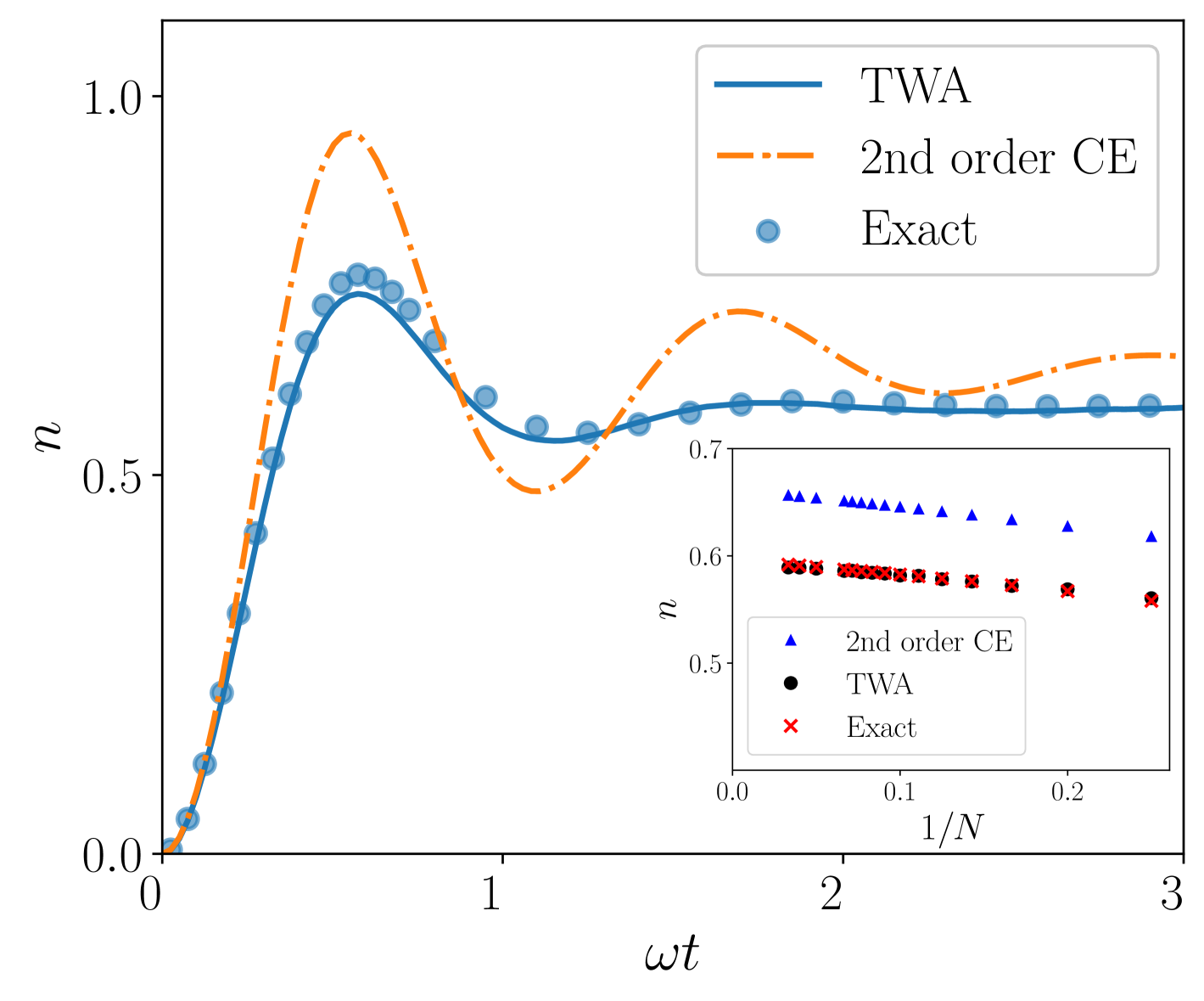
Figure 4: The population of the central site in the central spin model with $N=30$ as a function of time, starting from the central spin in its ground state and fully inverted satellite spins. TWA accurately captures the dynamics, whereas the second-order CE quickly deviates from the correct behavior. The inset shows the steady-state value for varying system sizes, where TWA remains accurate while CE fails across all system sizes. The parameters used are $\omega=\epsilon=\kappa$, $g/\omega=3$, $\gamma_{\downarrow}/\omega=1/2$, and $\gamma_{\uparrow}/\omega=3/2$. TWA results are obtained from $O(10^{5})$ trajectories.

III.4 Central spin model

For the purpose of refining our comparison between TWA and CE, we solve the central spin (CS) model, describing a single spin interacting collectively with an ensemble of $N$ satellite spins, which is a prototypical model of single spins or dilute spin ensembles interacting with many-body environments. Examples include nuclear magnetic resonance and nitrogen-vacancy centers in diamond [72, 73]. In the simplest case, the CS Hamiltonian is given by

$$\hat{H}=\frac{\omega}{2}\hat{\tau}^{z}+\frac{\epsilon}{2}\sum_{i=1}^{N}\hat{\sigma}^{z}_{i}+\frac{g}{\sqrt{N}}\sum_{i=1}^{N}\Big{(}\hat{\tau}^{+}\hat{\sigma}^{-}_{i}+\hat{\tau}^{-}\hat{\sigma}^{+}_{i}\Big{)},$$ (37)

where $\hat{\tau}^{\alpha}$ are Pauli operators of the central spin. In the following, we consider central spin loss ($\hat{L}^{k}=\hat{\tau}^{-}$) together with satellite spin loss ($\hat{L}^{\downarrow}_{i}=\hat{\sigma}^{-}_{i}$) and pumping ($\hat{L}^{\uparrow}_{i}=\hat{\sigma}^{+}_{i}$) with respective rates $\kappa$, $\gamma_{\downarrow}$, and $\gamma_{\uparrow}$. The CS model can be obtained from the TC model by replacing $\hat{a}\to\hat{\tau}^{-}$, and has the same symmetries. Due to the smaller local Hilbert space of the central spin versus the photon mode, we generally expect quantum fluctuations to be more important in the former case. For the TC model, as we go to larger values of $N$, a Gaussian state progressively becomes a better approximation for photons, improving the performance of CE. In contrast, no similar improvement in CE performance is expected when applied to the CS model (unless the central spin is large, of course). This is the key reason why the comparison between the dynamics of the TC and CS model is particularly instructive in assessing the validity of TWA versus CE.

We evaluate the dynamics of the CS model, after initializing the central and satellite spins in their ground and excited states, respectively. The equations of motion are given by

$$\derivative{t}\tau^{x} =-\omega\tau^{y}+\frac{g}{\sqrt{N}}\tau^{z}\sum_{i}s^{y}_{i}+\Big{(}\frac{\kappa}{2}\tau^{x}+\xi^{x}_{\kappa}\Big{)}\,\tau^{z},$$ (38)

$$\derivative{t}\tau^{y} =+\omega\tau^{x}-\frac{g}{\sqrt{N}}\tau^{z}\sum_{i}s^{x}_{i}+\Big{(}\frac{\kappa}{2}\tau^{y}+\xi^{y}_{\kappa}\Big{)}\,\tau^{z},$$ (39)

$$\derivative{t}\tau^{z} =+\frac{g}{\sqrt{N}}\Big{(}\tau^{y}\sum_{i}s^{x}_{i}-\tau^{x}\sum_{i}s^{y}_{i}\Big{)}-\frac{\kappa}{2}\Big{(}(\tau^{x})^{2}+(\tau^{y})^{2}\Big{)}$$

$$\qquad\qquad\qquad\qquad\qquad\qquad\quad-\big{(}\xi^{x}_{\kappa}\tau^{x}+\xi^{y}_{\kappa}\tau^{y}\big{)},$$ (40)

$$\derivative{t}s^{x}_{i} =-\epsilon s^{y}_{i}+\frac{g}{\sqrt{N}}\tau^{y}s^{z}_{i}+\frac{\gamma_{\downarrow}-\gamma_{\uparrow}}{2}s^{x}_{i}s^{z}_{i}+\big{(}\xi_{\downarrow,i}^{x}-\xi_{\uparrow,i}^{x}\big{)}s^{z}_{i},$$ (41)

$$\derivative{t}s^{y}_{i} =+\epsilon s^{x}_{i}-\frac{g}{\sqrt{N}}\tau^{x}s^{z}_{i}+\frac{\gamma_{\downarrow}-\gamma_{\uparrow}}{2}s^{y}_{i}s^{z}_{i}+\big{(}\xi_{\downarrow,i}^{y}+\xi_{\uparrow,i}^{y}\big{)}s^{z}_{i},$$ (42)

$$\derivative{t}s^{z}_{i} =+\frac{g}{\sqrt{N}}\big{(}\tau^{x}s^{y}_{i}-\tau^{y}s^{x}_{i}\big{)}-\frac{\gamma_{\downarrow}-\gamma_{\uparrow}}{2}\Big{(}(s^{x}_{i})^{2}+(s^{y}_{i})^{2}\Big{)}$$

$$\qquad\qquad\quad\qquad+\big{(}\xi^{x}_{\uparrow,i}-\xi^{x}_{\downarrow,i}\big{)}s^{x}_{i}-\big{(}\xi^{y}_{\uparrow,i}+\xi^{y}_{\downarrow,i}\big{)}s^{y}_{i}.$$ (43)

The noise variances are specified by

$$\overline{\xi^{\alpha}_{\kappa}(t)\xi^{\beta}_{\kappa}(t^{\prime})}=\kappa\,\delta_{\alpha\beta}\,\delta(t-t^{\prime}),$$ (44)

together with Eqs. (34) and (35). The TWA results for the central spin population, $n=(1+\langle\hat{\tau}^{z}\rangle)/2$, are shown in Fig. 4, demonstrating strong agreement with exact solutions for both transient dynamics and the steady state, with a relative error of $O(10^{-2})$. In contrast, second-order CE captures only the early-time dynamics but fails to predict the correct steady-state behavior for any system size, a limitation which persists even at higher orders of CE [23].

The last two examples illustrate the improved reliability of TWA compared to CE, the most widely used method for studying many-body quantum optical models. While for CE, going beyond the second order quickly increases the complexity of equations without guaranteed improvement [23, 24], the equations for TWA are the simple MF equations supplemented by noise, and grant access to higher-point correlation functions without extra effort. Incorporating inhomogeneities, which naturally arise in realistic scenarios, further highlights the advantage of TWA over CE. In the CS model, such inhomogeneities can manifest in both the satellite spin splittings ($\epsilon\to\epsilon_{i}$), coupling strengths ($g\to g_{i}$) or dissipation rates ($\gamma_{\uparrow\downarrow}\to\gamma_{\uparrow\downarrow,i}$). While TWA seamlessly accommodates these variations, CE faces a significant increase in computational complexity, with the number of equations growing from 4 to approximately $N(N+3)/2$ at second order, and even more for higher-order expansions.

III.5 Rydberg chain

So far, we have considered models with collective interactions, where only local dissipation disrupts their fully collective nature. Next, we examine two prominent examples of systems with strongly non-collective behavior, whose physics crucially depends on the probed time and length scales, and which therefore qualify as genuine strongly correlated many-particle systems. The next section is devoted to dissipation with non-trivial spatial structure. Here, we consider a driven-dissipative chain of spins with short-range Ising-like interactions, describing the physics of Rydberg atomic arrays, which is one the most versatile platforms for quantum simulation and quantum computing nowadays [74].

We consider the following Ising Hamiltonian

$$\hat{H}=\Omega\sum_{i}\hat{\sigma}_{i}^{x}+\frac{J}{4}\sum_{i}(1+\hat{\sigma}_{i}^{z})(1+\hat{\sigma}_{i+1}^{z}),$$ (45)

where $J$ is the strength of Rydberg interactions and $\Omega$ is the Rabi frequency. We consider local dephasing ($\hat{L}_{i}^{\kappa}=\hat{\sigma}_{i}^{z},$) and spin loss ( $\hat{L}_{i}^{\downarrow}=\hat{\sigma}_{i}^{-}$) with rates $\kappa$ and $\gamma_{\downarrow}$, respectively. Furthermore, we work with periodic boundary conditions. The evolution simulated with TWA shows good agreement with the exact solution both for transient dynamics and the steady state, with the exception of regimes where spontaneous decay is stronger than the typical energy scales of coherent dynamics.

Applying our formalism to Eq. (45) yields the following set of equations for classical variables

$$\derivative{t}s_{i}^{x} =-\frac{J}{2}\Big{(}2+s^{z}_{i-1}+s^{z}_{i+1}\Big{)}\,s_{i}^{y}+\Big{(}\frac{\gamma_{\downarrow}}{2}s_{i}^{x}+\xi_{\downarrow,i}^{x}\Big{)}\,s_{i}^{z}+2\eta_{i}s_{i}^{y},$$ (46)

$$\derivative{t}s_{i}^{y} =-2\Omega s^{z}_{i}+\frac{J}{2}\Big{(}2+s^{z}_{i-1}+s^{z}_{i+1}\Big{)}\,s_{i}^{x}+\Big{(}\frac{\gamma_{\downarrow}}{2}s_{i}^{y}+\xi_{\downarrow,i}^{y}\Big{)}\,s_{i}^{z}-2\eta_{i}s_{i}^{x},$$ (47)

$$\derivative{t}s_{i}^{z} =+2\Omega s_{i}^{y}-\Big{(}\frac{\gamma_{\downarrow}}{2}s^{x}_{i}+\xi_{\downarrow,i}^{x}\Big{)}\,s^{x}_{i}-\Big{(}\frac{\gamma_{\downarrow}}{2}s^{y}_{i}+\xi_{\downarrow,i}^{y}\Big{)}\,s^{y}_{i},$$ (48)

with dephasing ($\eta_{i}$) and spin loss ($\xi^{\alpha}_{\downarrow,i}$) noise variances given according to Table. 1.

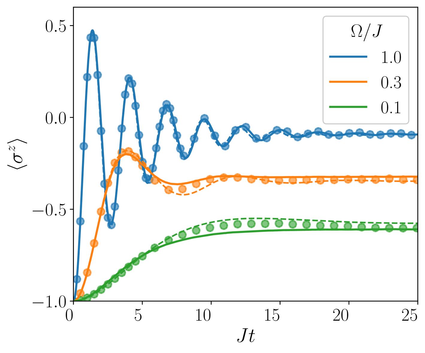
Figure 5: Dynamics of a Rydberg chain with size $N=10$, after being initialized in the atomic groundstate ($\ket{\downarrow}$). Both TWA (solid lines) and CE (dashes) are in agreement with the exact results (circles). The parameters are $\gamma_{\downarrow}/J=\kappa/J=0.1$. The exact dynamics and TWA have been respectively obtained by averaging over $O(10^{3})$ quantum and $O(10^{4})$ classical trajectories.

Figure 5 presents the dynamics of $\langle\hat{\sigma}^{z}\rangle$ for various driving strengths, as obtained from TWA, second-order CE, and the exact solution computed via the stochastic unraveling of quantum trajectories, using the QuTiP package of Ref. [8]. For $\Omega/J\gtrsim 0.1$, TWA closely matches the exact dynamics, whereas for weaker drives (not shown), its accuracy progressively decreases. CE performs similarly to TWA, and fails when interactions become very strong. Additionally, our TWA fails in the regime of strong spin loss ($\gamma_{\downarrow}\gtrsim\Omega$), where it is unable to accurately capture the system’s dark state, as previously discussed in Sec. III.2. Notably, by adding spin dephasing, convergence improves significantly.

Notably, for this problem, implementing TWA is simpler than CE, which requires tracking all first-order ($\langle\hat{\sigma}^{\alpha}_{i}\rangle$) and second-order ($\langle\hat{\sigma}^{\alpha}_{i}\hat{\sigma}^{\beta}_{j}\rangle$) cumulants to obtain a closed system of equations. To handle the large number of the resulting equations, we used the QuantumCumulants.jl package [21] to obtain CE results. However, extending CE to higher orders proved considerably more computationally expensive than both TWA and the exact solution, even for a system of size $N=10$. This inefficiency stems in part from the fact that the current CE implementation in Ref. [21] cannot exploit the translation symmetry of the problem and calculates many redundant cumulants. We also note that translation symmetry is present only for homogeneous systems and under periodic boundary conditions, which do not apply in many situations. Without leveraging the translation symmetry, the symbolic evaluation of second-order CE for $N\gtrsim 20$ already exceeds the memory capacity of a personal computer. In contrast, TWA allows seamless simulation of dynamics for hundreds of spins on a desktop and several thousand on a supercomputer.

III.6 Correlated decay

As the final example of this work, we consider decay processes with a non-diagonal dissipation matrix in the atomic basis:

$$\Gamma_{ij}\neq\gamma_{i}\,\delta_{ij}.$$ (49)

A special case corresponds to fully collective decay [75, 76], where $\Gamma_{ij}$ is uniform, and the analysis is simplified by recasting dissipation in terms of a collective jump operator $\hat{L}_{\mathrm{col}}=\sum_{i}\hat{\sigma}^{-}_{i}$. This leads to the Dicke superradiance of atomic ensembles, whose key features can be captured using simple approaches such as MF. Here, we are interested in regimes away from the limits of independent and fully collective decay. While this regime can be realized in different contexts [77, 78, 79, 80, 81, 82], here we focus on the particular example of correlated emission in sub-wavelength arrays of atoms.

The dynamics of a coherently driven atomic array placed in the electromagnetic (EM) vacuum can be expressed using the Lindblad master equation [77]

$$\derivative{t}\hat{\rho}=-i\,[\hat{H},\hat{\rho}]+\sum_{ij=1}^{N}\Gamma_{ji}\,\Big{(}\hat{\sigma}_{i}^{-}\hat{\rho}\hat{\sigma}_{j}^{+}-\frac{1}{2}\{\hat{\sigma}_{j}^{+}\hat{\sigma}_{i}^{-},\hat{\rho}\}\Big{)}.$$ (50)

The Hamiltonian reads

$$\hat{H}=\omega_{z}\sum_{i=1}^{N}\hat{\sigma}_{i}^{z}+\Omega\sum_{i=1}^{N}\hat{\sigma}^{x}_{i}+\sum_{ij=1}^{N}J_{ij}\,\hat{\sigma}_{i}^{+}\hat{\sigma}_{j}^{-},$$ (51)

where $J_{ij}$ describes dipolar interaction between atoms, $\omega_{z}$ is the effective detuning which also includes the Lamb’s shift due to coupling to EM modes, and $\Omega$ is the Rabi frequency. The interaction and dissipation matrices can be obtained from (in units where $\hbar\equiv 1$)

$$J_{ij} =-\omega^{2}\,\bar{\bm{p}}\cdot\mathrm{Re}\,\bm{G}\big{(}\bm{r_{i}}-\bm{r_{j}},\omega\big{)}\cdot\bm{p},$$ (52)

$$\Gamma_{ij} =+2\omega^{2}\,\bar{\bm{p}}\cdot\mathrm{Im}\,\bm{G}\big{(}\bm{r_{i}}-\bm{r_{j}},\omega\big{)}\cdot\bm{p},$$ (53)

where $\bm{p}$ is the atomic dipole, and $\bm{G}$ is the Green’s function of EM modes [83]. In the vacuum we have

$$\mathbf{G}_{0}(\mathbf{r},\omega)=\dfrac{\mu_{0}\,e^{ikr}}{4\pi k^{2}r^{3}}\Big{[}(k^{2}r^{2}+ikr-1)\mathds{1}+(3-3ikr-k^{2}r^{2})\frac{\mathbf{r}\otimes\mathbf{r}}{r^{2}}\Big{]},$$ (54)

where $\omega$ is the optical transition frequency, $\mu_{0}$ is the vacuum permeability, and $k=\omega/c$ is the momentum of emitted photons. The physics of such a system crucially depends on the timescales and length-scales under consideration. In particular, the ratio of the inter-atomic distance $a$ to the wavelength of emitted light $\lambda\equiv 2\pi/k$ tunes the degree of collective behavior in the system. For $a\lesssim\lambda$, subsystems smaller than $\lambda$ can emit superradiantly, if initialized in a sufficiently excited state, while a fraction of the energy may remain trapped in the system for extended durations due to the existence of subradiant (evanescent) modes, depending on the system’s geometry [77, 79, 84]. In the limit $a\gtrsim\lambda$, correlations become unimportant and atoms emit independently with the rate

$$\Gamma_{0}=\lim_{j\to i}\Gamma_{ij}=\frac{\mu_{0}\omega^{3}|\bm{p}|^{2}}{3\pi c}.$$ (55)

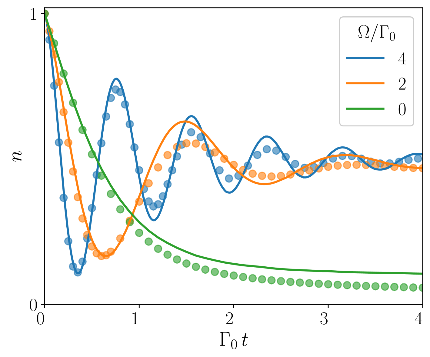
Figure 6: Dynamics of the average excitation number of a chain of $N=8$ emitters, subject to correlated decay and Rabi driving. Solid lines and circles respectively correspond to TWA and the exact solution. The lattice spacing is $a=\lambda/5$, and the averages are taken over $O(10^{4})$ trajectories.

We simulate the dynamics of a one-dimensional array using our approach. The equations of motion for classical spin variables read (Sec III.1)

$$\derivative{t}s_{i}^{x} =-2\omega_{z}s_{i}^{y}+s_{i}^{z}\sum_{j}J_{ij}s_{i}^{y}+\frac{1}{2}s_{i}^{z}\sum_{j}\Gamma_{ij}s_{j}^{x}+\xi_{i}^{x}s_{i}^{z},$$ (56)

$$\derivative{t}s_{k}^{i} =+2\omega_{z}s_{i}^{x}-2\Omega s_{i}^{z}-s_{i}^{z}\sum_{j}J_{ij}s_{j}^{x}+\frac{1}{2}s_{i}^{z}\sum_{j}\Gamma_{ij}s_{j}^{y}+\xi_{i}^{y}s_{i}^{z},$$

$$\derivative{t}s_{i}^{z} =+2\Omega s_{i}^{y}+\sum_{j}J_{ij}\,\Big{(}s^{y}_{i}s_{j}^{x}-s_{i}^{x}s_{j}^{y}\Big{)}-\frac{1}{2}\sum_{j}\Gamma_{ij}\,\Big{(}s_{i}^{x}s_{j}^{x}+s_{i}^{y}s_{j}^{y}\Big{)}$$

$$\qquad\qquad\qquad\ \qquad\qquad\qquad\quad-\left(\xi_{i}^{x}s_{i}^{x}+\xi_{i}^{y}s_{i}^{y}\right),$$

with non-local noise variances

$$\overline{\xi^{\alpha}_{i}(t)\,\xi^{\beta}_{j}(t^{\prime})}=\Gamma_{ij}\,\delta_{\alpha\beta}\,\delta(t-t^{\prime}).$$ (57)

Numerically, non-local noises can be sampled by diagonalizing the dissipation matrix

$$\hat{\Gamma}\cdot\bm{v}^{j}=\gamma_{j}\,\bm{v}^{j},\quad 1\leq j\leq N,$$ (58)

with eigenvectors $\bm{v}^{j}$ and their corresponding eigenvalues $\gamma_{i}\geq 0$. We then define the collective noise variables according to

$$\overline{\eta^{\alpha}_{i}(t)\,\eta^{\beta}_{j}(t^{\prime})}=\gamma_{i}\,\delta_{ij}\,\delta_{\alpha\beta}\,\delta(t-t^{\prime}),$$ (59)

such that the noise tensor in the site-basis can be obtained from the linear superposition of the collective noises via

$$\xi_{i}^{\alpha}=\sum_{j=1}^{N}v^{\,j}_{i}\,\eta^{\alpha}_{j}.$$ (60)

In Fig. 6, we compare the predictions of TWA for a sub-wavelength chain of driven atoms ($a=\lambda/5$) to exact results. We observe that for sufficiently strong driving relative to $\Gamma_{0}$, TWA accurately captures the system’s dynamics. For weak driving, it becomes less reliable and, as in the single-spin case discussed in Sec. III.2, predicts an incorrect steady-state population. However, we remark that the accuracy of TWA for this problem cannot be assessed by a single ratio such as $\Omega/\Gamma_{0}$, as it depends crucially on the spatial structure of the eigenvectors in Eq. (58). Importantly, the collective decay rates in Eq. (58) span a broad range of energy scales, with $\Gamma_{0}$ representing only their average, $\Gamma_{0}=\sum_{i}\gamma_{i}/N$. Notably, in the limit $a\ll\lambda$, where the largest eigenvalue of $\Gamma$ corresponds to the most superradiant mode, TWA correctly captures the superradiant burst even in the absence of a drive ($\Omega=0$). To illustrate that, we plot the normalized emission rate

$$R(t) \equiv\frac{1}{N\Gamma_{0}}\derivative{t}n=\frac{1}{N\Gamma_{0}}\sum_{ij}\Gamma_{ij}\langle\sigma_{i}^{+}\sigma_{j}^{-}\rangle=$$ (61)

$$=\frac{1}{N\Gamma_{0}}\sum_{ij}\left[\frac{1}{N_{\text{tot}}}\sum_{n=1}^{N_{\text{tot}}}\Gamma_{ij}s_{i,n}^{+}s_{j,n}^{-}+\frac{\Gamma_{0}}{2N_{\text{tot}}}\sum_{n=1}^{N_{\text{tot}}}s_{i,n}^{z}\delta_{ij}\right]$$

for different values of $a$ and $N=10$ in Fig. 7. In the third step of  (61) we transited from operators to classical variables. For all simulations, TWA captures essential features of the dynamics, and for small atomic separations, $a=\lambda/10$, it matches quantitatively the exact numerical dynamics of $R(t)$. In the inset, we plot dynamics up to $N=1000$ atoms, but larger system sizes are also at reach with our approach. Importantly, TWA requires solution of $3N$ stochastic differential equations, and the operational capabilities of the method are set mostly by the accessible memory resources. On the other hand, third-order CE which have been employed to simulate correlated emission recently [20], would saturate faster, as the number of equations to be solved scales like $N^{3}$. Furthermore, the intricacy of higher order CE (cf. Appendix of  [20]) compared to Eqs. (56) would set a further obstacle to apply cumulants to other Lindbladians with non-trivial spatial structure [80].

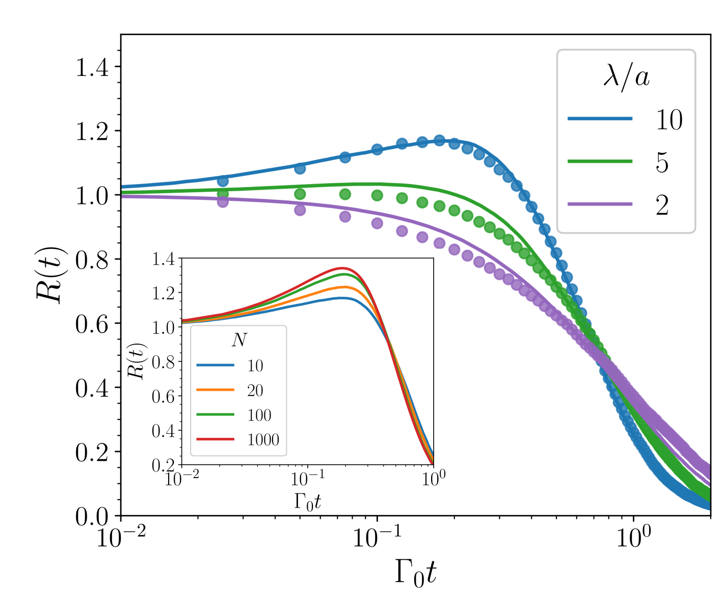
Figure 7: Emission rate of an initially inverted atomic chain with size $N=10$ as a function of time and for different values of lattice spacing. TWA (solid lines) captures the superradiant burst and matches exact numerics (circles). Inset: TWA results for the emission rate of a fully inverted atomic chain with $\lambda/a=10$ as a function of time and for different system sizes.

IV Conclusions and outlook

The simplicity of our approach, combined with its accuracy in solving key many-body quantum optics models, strongly suggests its potential as an essential tool in every AMO physicist’s theoretical toolbox. Given the straightforward transition from the Lindblad master equation to the semiclassical equations of motion, developing a dedicated numerical framework to further streamline its use, similar to QuTiP for exact dynamics [8] and QuantumCumulants.jl for CE [21], is completely within reach. Such a framework could, in principle, leverage parallel computing techniques to efficiently explore problems in the true many-body limit, encompassing thousands of degrees of freedom.

This work can be extended by incorporating higher-order quantum corrections into the approximation. In this regard, our field-theoretic derivation provides a foundation for systematically advancing the semiclassical expansion. A similar approach has been previously explored for TWA in isolated systems [45], where next-order quantum corrections were introduced via quantum jumps, distinct from Lindblad jump operators, which are stochastically applied to trajectories. Including higher order corrections in our case follows the same logic. The connection between the truncated Wigner approximation (TWA) and the semiclassical limit of the Langevin equation lies at the heart of the transparency and flexibility of the approach presented in this work. This can be seen as a clear success of the Keldysh formalism, as we are not aware of any more straightforward derivations of this connection. Notably, this appears to be one of the cases where Keldysh field theory is not merely a way to reframe established results in a different language but instead provides a genuine systematic advantage over more elementary techniques.

Another possibility is to revisit the fundamental origins of dissipation. Specifically, when the environment is structured or non-Markovian, it modifies both the dissipative and stochastic components of the spin dynamics in (5) (cf. Refs. [59, 85, 86]). This effect can be systematically derived using the same Keldysh path integral formalism employed in this work. In this framework, the damping term of dissipation is replaced by a convolution of dynamical variables with a memory function, $\Gamma_{ij}(t-t^{\prime})$, while white noise is replaced by colored noise. Consequently, spin dynamics is governed by a set of stochastic integro-differential equations with temporally non-local deterministic terms, which are still amenable to efficient numerical techniques. This approach provides a powerful tool for studying spin relaxation in structured environments, such as nitrogen-vacancy (NV) centers in diamond [87, 88, 89, 90] or superconducting qubits [91].

In recent years, there has been a growing body of work on solving driven dissipative spin models using semiclassical methods [55, 57, 56, 63, 92, 54, 93]. The increasing success of these approaches, as also documented in our work, including their ability to fit experimental data, raises a fundamental question in the field of driven open systems: Which aspects of dynamics are quantum-dominated when many-body systems are strongly coupled to their environments? A qualitative breakdown of TWA (or also of CE) appears to be a necessary condition if we wish to realize many-body entangled states under drive and dissipation. We emphasize that we are concerned here with identifying significant qualitative differences between results from the TWA and a genuine quantum mechanical description, rather than merely addressing a quantitative discrepancy which is not unreasonable to occur, as we have discussed at length in this work. Of course, this also naturally points to the need for advanced models capable of treating dissipative many-body systems with dominant quantum effects. Such models may include the development of tensor networks, variational states [31, 32, 33, 38], or field-theoretical approaches [4, 40, 41], as mentioned in the Introduction.

Viewed in this light, the question of whether TWA can capture dissipative quantum dynamics extends beyond a technical matter. Its breakdown would signal the emergence of entangled states that cannot be efficiently simulated with classical resources or the successful synthesis of phases of matter dominated by extended strong quantum correlations. We therefore anticipate that identifying models where TWA fails and more refined approaches are required will be key to advancing many-body AMO physics into a new era.

Appendix A Derivation of semiclassical equations of motion

In this Appendix, we systematically obtain the semiclassical equations of motion for dissipative spins, which were presented in the main text. Our approach, based on the Keldysh formalism of quantum field theory, is a natural extension of a similar derivation for unitary spin dynamics [47, 45].

Keldysh field theory is an alternative path-integral representation of quantum mechanics, and is particularly advantageous for non-equilibrium systems. [35]. The conventional Feynman path-integral, whose lower and upper limits respectively correspond to the initial ($t_{i}$) and final ($t_{f}$) times of the evolution, is given by

$$S_{\mathrm{Feynman}}=\int_{t_{i}}^{t_{f}}L[\psi(t)]\,dt,$$ (62)

where $\psi$ represents the degrees of freedom in the system. Instead, the Keldysh path-integral is defined along a closed time-contour $\mathcal{C}$:

$$S_{\mathrm{Keldysh}}=\int_{\mathcal{C}}L[\psi(t_{c})]\,dt_{c},$$ (63)

where $\mathcal{C}$ is specified by the path $t_{i}\to t_{f}\to t_{i}$. Therefore, we can write

$$S_{\mathrm{Keldysh}}=\int_{t_{i}}^{t_{f}}L[\psi^{+}(t)]\,dt-\int_{t_{f}}^{t_{i}}L[\psi^{-}(t)]\,dt,$$ (64)

which means that one can work with a normal temporal integration at the expense of doubling the number of fields, corresponding to integration along the forward ($+$) and backward ($-$) branches of $\mathcal{C}$. The expectation values of operators can be obtained from

$$\expectationvalue{O(t)}=\int\mathbf{D}[\psi]\,P_{0}[\psi_{0}]\,O(t)\,e^{iS_{\mathrm{Keldysh}}},$$ (65)

where $P_{0}[\psi]$ is the initial distribution of the fields. The advantage of working with a doubled number of fields is the ability to address non-equilibrium phenomena, in a wide range of problems from condensed matter physics to high energy physics and cosmology [35]. Recently, it has been extended to open quantum systems with Lindblad dynamics [4], allowing the study of, for instance, the dissipative Dicke model [94, 95] as well as the discovery of non-equilibrium universality classes [5, 96].

Below, we present a step-by-step explanation of our derivation. Our discussion remains general, without specifying a particular dissipation channel. Moreover, we maintain an exact treatment throughout the derivation, applying the semiclassical approximation only at the final stage.

A.1 Exact path-integral formulation of the problem

Below, we apply a series of transformations to the Keldysh action of the original model, mapping the problem onto a field theory with explicit noise terms. In the next section, we will use this new formulation to derive the rules of dissipative TWA.  

Constructing the Keldysh action– The Keldysh action consists of a coherent part, corresponding to the Hamiltonian dynamics, and a dissipative part, corresponding to the Lindblad dynamics:

$$S=S_{c}+S_{d}.$$ (66)

The coherent part of the action can be written as

$$S_{c}=S_{0}+S_{H},$$ (67)

where $S_{0}$ is determined by the algebra of the degrees of freedom in the system and contains time-derivatives [97]. $S_{H}$ is explicitly given by the Hamiltonian as

$$S_{H}=-\int dt\,(H^{+}-H^{-}),$$ (68)

where $H^{\pm}$ is the Hamiltonian evaluated on the forward and backward branches of the Keldysh contour. The dissipative part of the action, corresponding to the Lindbladian in Eq. (1), is given by (see Ref. [4])

$$S_{d}=-i\sum_{i}\frac{\gamma_{i}}{2}\int\mathrm{d}t\left(2L_{i}^{+}\bar{L}_{i}^{-}-L_{i}^{-}\bar{L}_{i}^{-}-L_{i}^{+}\bar{L}_{i}^{+}\right)$$ (69)

where $L_{i}$ are the fields corresponding to the jump operators. Without loss of generality, we have considered a diagonal matrix $\Gamma_{ij}=\delta_{ij}\gamma_{i}$, since the dissipation matrix can always be written in diagonal form after a linear transformation of jump operators.

‘Recovering’ the bath– For technical reasons that will become evident later, we perform a procedure akin to recovering the bath degrees of freedom—in essence, the inverse of integrating out the bath. However, no additional information about the bath is needed beyond what is provided in Eq. (69). Mathematically, this is accomplished through a Hubbard-Stratonovich transformation which reverses the process of evaluating a Gaussian integral [97, 35]:

$$e^{-\bm{u}^{\dagger}\cdot\hat{A}\cdot\bm{v}}\propto\int\mathbf{D}[\bm{x}^{\dagger},\bm{x}]\,e^{-\bm{x}^{\dagger}\cdot\hat{A}^{-1}\cdot\bm{x}+i\bm{x}^{\dagger}\cdot\bm{v}+i\bm{u}^{\dagger}\cdot\bm{x}}.$$ (70)

We write the dissipative action in Eq. (69) in the matrix form

$$S_{d}=\sum_{i}\int dt\,\begin{pmatrix}\bar{L}^{+}_{i}&-\bar{L}^{-}_{i}\end{pmatrix}\begin{pmatrix}i\gamma_{i}/2&0\\ i\gamma_{i}&i\gamma_{i}/2\end{pmatrix}\begin{pmatrix}L^{+}_{i}\\ -L^{-}_{i}\end{pmatrix}.$$ (71)

We then use Eq. (70) to get $e^{iS_{d}}=\int\bm{D}[\bar{\Phi}^{\pm},\Phi^{\pm}]\,e^{iS_{B}+iS_{sB}}$, where

$$S_{B}=\sum_{i}\int dt\,\begin{pmatrix}\bar{\Phi}^{+}_{i}&\bar{\Phi}^{-}_{i}\end{pmatrix}\begin{pmatrix}2i/\gamma_{i}&0\\ -4i/\gamma_{i}&2i/\gamma_{i}\end{pmatrix}\begin{pmatrix}\Phi^{+}_{i}\\ \Phi^{-}_{i}\end{pmatrix},$$ (72)

is the action of Markovian bath and

$$S_{sB}=\sum_{i}\int dt\,\big{(}\bar{\Phi}^{+}_{i}L^{+}_{i}+\bar{L}^{+}_{i}\Phi^{+}_{i}-\bar{\Phi}^{-}_{i}L^{-}_{i}-\bar{L}^{-}_{i}\Phi^{-}_{i}\big{)},$$ (73)

describes the system-bath coupling. Together, Eqs. (67), (72) and (73) govern the dynamics of a system of spins coupled to the ‘fictitious’ bath degrees of freedom, which are expressed by the fields $\Phi_{i}$.  

Separating quantum fluctuations– The next step involves separating the fluctuating part of the fields due to quantum effects. This is done by defining the forward and backward fields in terms of classical and quantum fields, using the following linear transformation [35]

$$\Phi^{\pm}_{i} =\Phi^{c}_{i}\pm\Phi^{q}_{i},$$ (74)

$$L^{\pm}_{i} =L^{c}_{i}\pm L^{q}_{i}.$$ (75)

The action of the bath in the new basis is given by

$$S_{B}=\sum_{i}\int\,\frac{4i}{\gamma_{i}}\big{(}\bar{\Phi}^{q}_{i}\Phi^{c}_{i}-\bar{\Phi}^{c}_{i}\Phi^{q}_{i}+2\bar{\Phi}^{q}_{i}\Phi^{q}_{i}\big{)}\,dt,$$ (76)

and the system-bath coupling reads as

$$S_{sB}=\sum_{i}\int dt\,\big{(}2\bar{\Phi}^{c}_{i}L^{q}_{i}+2\bar{\Phi}^{q}_{i}L^{c}_{i}+2\bar{L}^{c}_{i}\Phi^{q}_{i}+2\bar{L}^{q}_{i}\Phi^{c}_{i}\big{)}.$$ (77)

We note that, the change of basis to the classical and quantum components naturally leads to the Wigner transformation of the initial distribution function in Eq. (65) [47, 45].  

Identifying the noise– In the next step, we identify and isolate the noisy contribution to dissipative dynamics. This is step similar to the derivation of the Langevin’s equation [35], and is achieved by noting that the $\bar{\Phi}^{q}\Phi^{q}$ term in Eq. (76) can be written as

$$e^{-\sum_{i}\frac{8}{\gamma_{i}}\int|\Phi^{q}_{i}|^{2}\,dt}\propto\overline{e^{\sum_{i}\frac{2i}{\gamma_{i}}\int dt\,(\bar{\Phi}^{q}_{i}\xi_{i}+\bar{\xi}_{i}\Phi^{q}_{i})\,dt}},$$ (78)

where the average is taken with respect to the complex Gaussian noise $\xi(t)$ given by the following distribution

$$\mathcal{P}[\bar{\xi}_{i},\xi_{i}]\propto\exp(-\sum_{i}\frac{1}{2\gamma_{i}}\int|\xi_{i}(t)|^{2}\,dt).$$ (79)

After substituting Eq. (78) in Eq. (76), we get

$$S_{B}+S_{sB}=\sum_{i}\int dt\,\Big{[}\bar{\Phi}^{q}_{i}\Big{(}\frac{4i}{\gamma_{i}}\Phi^{c}_{i}+\frac{2}{\gamma_{i}}\xi_{i}+2{L}^{c}_{i}\Big{)}+\mathrm{c.c.}\Big{]}\\ +\sum_{i}\int dt\,\Big{(}2\bar{\Phi}^{c}_{i}L^{q}_{i}+2\bar{L}^{q}_{i}\Phi^{c}_{i}\Big{)}.$$ (80)

Note that $\Phi^{q}$ only appears linearly in the first line. As the result, the functional integral over $(\bar{\Phi}^{q},\Phi^{q})$ can be evaluated, yielding a Dirac delta:

$$\int\mathbf{D}[\bar{\Phi}^{q}_{i},\Phi^{q}_{i}]e^{i\sum_{i}\int dt\,\Big{[}\bar{\Phi}^{q}_{i}\big{(}\frac{4i}{\gamma_{i}}\Phi^{c}_{i}+\frac{2}{\gamma_{i}}\xi_{i}+2{L}^{c}_{i}\big{)}+\mathrm{c.c.}\Big{]}}\\ \propto\delta\Big{(}\frac{4i}{\gamma_{i}}\Phi^{c}_{i}+\frac{2}{\gamma_{i}}\xi_{i}+2\bar{L}^{c}_{i}\Big{)}.$$ (81)

Since $\Phi^{q}$ has been integrated out and we are left only with the classical field $\Phi^{c}$, for brevity, we ignore its classical index and define

$$\Phi_{i}\equiv-i\Phi^{c}_{i}.$$ (82)

The delta function determines the value of $\Phi_{i}$ as

$$\Phi_{i}=\frac{\gamma_{i}}{2}L^{c}_{i}+\frac{1}{2}\xi_{i}.$$ (83)

We rewrite the jump fields in the second line of Eq. (80) in the contour basis by using $2L^{q}_{i}=L^{+}_{i}-L^{-}_{i}$. Then, these terms can be absorbed into the Hamiltonian contribution in Eq. (68) to get

$$\tilde{S}_{H}=-\int dt\,(\tilde{H}^{+}-\tilde{H}^{-}),$$ (84)

where $\tilde{H}$ is the complex effective Hamiltonian, which is $H$ shifted by a coupling to the jump fields:

$$\tilde{H}^{\pm}\equiv H^{\pm}-i\sum_{i}\big{(}\bar{L}^{\pm}_{i}\Phi_{i}-\bar{\Phi}_{i}L^{\pm}_{i}\big{)}.$$ (85)

One might be tempted to elevate Eq. (85) to operator level. However, this is not possible as the field $\Phi$ depends on the jump fields (Eq. (83)) on both of the Keldysh contours, so $\tilde{H}^{+}$ ($\tilde{H}^{-}$) contains fields on both forward and backward contours.

So far, our treatment has been exact, and the full solution of the problem still requires evaluating the above noisy field theory. However, the new formulation of the problem is very convenient for semiclassical approximations, as we will show below.

A.2 Semiclassical approximation

To obtain the semiclassical approximation, we look at the whole Keldysh path-integral that we obtained in the previous section:

$$\int\mathbf{D}[\bar{\Phi},\Phi]\,\int\mathbf{D}[\psi^{\pm}]\,P_{0}[\psi^{\pm}_{0}]\,\\ \times\overline{\delta\left(\Phi_{i}-\frac{\gamma_{i}}{2}L^{c}_{i}-\frac{1}{2}\xi_{i}\right)\,e^{iS_{0}+i\tilde{S}_{H}}},$$ (86)

where the long bar is the average with respect to noise distribution in Eq. (79), and we have kept the delta function, which imposes the value of $\Phi$, explicit. In this formulation, the semiclassical approximation is straightforward: for each realization of the noise, we apply TWA to the path integral and then, take the average over different noise realizations. The former step yields the classical equations of motion averaged over different trajectories [45]:

$$\int\mathbf{D}[\psi^{\pm}]\,P_{0}[\psi^{\pm}_{0}]\,e^{iS_{0}+i\tilde{S}_{H}}\\ \approx\int\mathbf{D}[\psi^{c}]\,P_{0}^{c}[\psi_{0}^{c}]\,\delta\big{(}\dot{\psi}^{c}-\{\psi^{c},\tilde{H}^{c}\}_{p}\big{)},$$ (87)

where $P^{c}_{0}$ is the initial semiclassical (quasi-)distribution function, and $\{A,B\}_{p}$ is the Poisson’s bracket. For brevity, we drop the classical index of all the fields as their quantum components no longer appear in Eq. (87). Therefore, Eq. (86) is approximated as

$$\int\mathbf{D}[\bar{\Phi},\Phi]\,\mathbf{D}[\psi]\,P_{0}^{c}[\psi_{0}]\,\\ \times\overline{\delta\big{(}\dot{\psi}-\{\psi,\tilde{H}\}_{p}\big{)}\,\delta\big{(}\Phi_{i}-\frac{\gamma_{i}}{2}L^{c}_{i}-\frac{1}{2}\xi_{i}\big{)}}.$$ (88)

The key point to remember is that, the first delta function on the RHS of the above equation yields the classical equations of motion for each trajectory while treating the field $\Phi$ in $\tilde{H}$ as a number, rather than an active dynamical variable. Afterwards, the second delta function imposes the value of $\Phi$ in the equations of motion. In other words,$\Phi$ should not be treated as a dynamical variable, and its Poisson bracket with any other variable must be assumed to vanish, when we derive the classical equations of motion.

We also note that, in the case of spins, we never had to explicitly use their path-integral representation. While one could, in principle, adopt a specific spin representation from the outset, such as spin-coherent states or Schwinger bosons, the final result always reduces to the form of Eq. (86), yielding nothing beyond the classical equations of motion [45].  

Based on the discussion above, we arrive at the following rules for dissipative TWA:  

1. Find the equations of motion for the following classical complex Hamiltonian

   $$\tilde{H}=H-i\sum_{i}(\bar{L}_{i}\Phi_{i}-\bar{\Phi}_{i}L_{i}),$$ (89)

2. Substitute the self-consistent field $\Phi$ in the equations of motion according to

   $$\Phi_{i}=\frac{1}{2}\gamma_{i}L_{i}+\frac{1}{2}\xi_{i},$$ (90)

   where $\xi_{i}$ is a Gaussian noise defined by

   $$\overline{\xi_{i}(t)}=0,\quad\overline{\xi_{i}(t)\bar{\xi}_{i}(t^{\prime})}=2\,\gamma_{i}\delta(t-t^{\prime}).$$ (91)

   Note that $\Phi_{i}$ has to be substituted only after obtaining the equations of motion.

3. Solve the equations of motion for different trajectories and different noise realizations until appropriate convergence is achieved.

The extension to the general case of Eq. (1) with non-diagonal dissipation follows the same line of arguments, whose result was given in the text.

References

- Fazio et al. [2024] R. Fazio, J. Keeling, L. Mazza, and M. Schiro, Many-body open quantum systems, arXiv preprint arXiv:2409.10300 (2024).
- Haroche and Raimond [2006] S. Haroche and J.-M. Raimond, Exploring the quantum: atoms, cavities, and photons (Oxford university press, 2006).
- Reitz et al. [2022] M. Reitz, C. Sommer, and C. Genes, Cooperative quantum phenomena in light-matter platforms, PRX Quantum 3, 010201 (2022).
- Sieberer et al. [2016] L. M. Sieberer, M. Buchhold, and S. Diehl, Keldysh field theory for driven open quantum systems, Reports on Progress in Physics 79, 096001 (2016).
- Sieberer et al. [2023] L. M. Sieberer, M. Buchhold, J. Marino, and S. Diehl, Universality in driven open quantum matter, arXiv preprint arXiv:2312.03073 (2023).
- Mivehvar et al. [2021] F. Mivehvar, F. Piazza, T. Donner, and H. Ritsch, Cavity qed with quantum gases: new paradigms in many-body physics, Advances in Physics 70, 1 (2021), https://doi.org/10.1080/00018732.2021.1969727 .
- Breuer and Petruccione [2007] H.-P. Breuer and F. Petruccione, The Theory of Open Quantum Systems (Oxford University Press, 2007).
- Johansson et al. [2013] J. Johansson, P. Nation, and F. Nori, Qutip 2: A python framework for the dynamics of open quantum systems, Computer Physics Communications 184, 1234 (2013).
- Daley [2014] A. J. Daley, Quantum trajectories and open many-body quantum systems, Advances in Physics 63, 77 (2014).
- Chiocchetta et al. [2021] A. Chiocchetta, D. Kiese, C. P. Zelle, F. Piazza, and S. Diehl, Cavity-induced quantum spin liquids, Nature Communications 12, 5901 (2021).
- Mann et al. [2025] C.-R. Mann, M. Oehlgrien, B. Jaworowski, G. Calajo, J. Marino, K. S. Choi, and D. E. Chang, in preparation (2025).
- Marino et al. [2022] J. Marino, M. Eckstein, M. S. Foster, and A. M. Rey, Dynamical phase transitions in the collisionless pre-thermal states of isolated quantum systems: theory and experiments, Reports on Progress in Physics 85, 116001 (2022).
- Kirton and Keeling [2017] P. Kirton and J. Keeling, Suppressing and restoring the Dicke superradiance transition by dephasing and decay, Phys. Rev. Lett. 118, 123602 (2017).
- Chelpanova et al. [2024] O. Chelpanova, K. Seetharam, R. Rosa-Medina, N. Reiter, F. Finger, T. Donner, and J. Marino, Dynamics of spin-momentum entanglement from superradiant phase transitions, Phys. Rev. Res. 6, 033193 (2024).
- Chelpanova et al. [2023] O. Chelpanova, A. Lerose, S. Zhang, I. Carusotto, Y. Tserkovnyak, and J. Marino, Intertwining of lasing and superradiance under spintronic pumping, Phys. Rev. B 108, 104302 (2023).
- Kirton et al. [2019] P. Kirton, M. M. Roses, J. Keeling, and E. G. Dalla Torre, Introduction to the dicke model: From equilibrium to nonequilibrium, and vice versa, Advanced Quantum Technologies 2, 1800043 (2019).
- Defenu et al. [2023] N. Defenu, T. Donner, T. Macrì, G. Pagano, S. Ruffo, and A. Trombettoni, Long-range interacting quantum systems, Rev. Mod. Phys. 95, 035002 (2023).
- Kirton and Keeling [2018] P. Kirton and J. Keeling, Superradiant and lasing states in driven-dissipative dicke models, New Journal of Physics 20, 015009 (2018).
- Robicheaux and Suresh [2021] F. Robicheaux and D. A. Suresh, Beyond lowest order mean-field theory for light interacting with atom arrays, Physical Review A 104, 023702 (2021).
- Rubies-Bigorda et al. [2023] O. Rubies-Bigorda, S. Ostermann, and S. F. Yelin, Characterizing superradiant dynamics in atomic arrays via a cumulant expansion approach, Phys. Rev. Res. 5, 013091 (2023).
- Plankensteiner et al. [2022] D. Plankensteiner, C. Hotter, and H. Ritsch, Quantumcumulants. jl: A julia framework for generalized mean-field equations in open quantum systems, Quantum 6, 617 (2022).
- Holzinger et al. [2024] R. Holzinger, O. Rubies-Bigorda, S. F. Yelin, and H. Ritsch, Symmetry based efficient simulation of dissipative quantum many-body dynamics in subwavelength quantum emitter arrays, arXiv preprint arXiv:2409.02790 (2024).
- Fowler-Wright et al. [2023] P. Fowler-Wright, K. B. Arnardóttir, P. Kirton, B. W. Lovett, and J. Keeling, Determining the validity of cumulant expansions for central spin models, Phys. Rev. Res. 5, 033148 (2023).
- Paškauskas and Kastner [2012] R. Paškauskas and M. Kastner, Equilibration in long-range quantum spin systems from a bbgky perspective, Journal of Statistical Mechanics: Theory and Experiment 2012, P02005 (2012).
- Orús [2014] R. Orús, A practical introduction to tensor networks: Matrix product states and projected entangled pair states, Annals of Physics 349, 117 (2014).
- Weimer et al. [2021] H. Weimer, A. Kshetrimayum, and R. Orús, Simulation methods for open quantum many-body systems, Rev. Mod. Phys. 93, 015008 (2021).
- Vidal [2003] G. Vidal, Efficient classical simulation of slightly entangled quantum computations, Phys. Rev. Lett. 91, 147902 (2003).
- Vidal [2004] G. Vidal, Efficient simulation of one-dimensional quantum many-body systems, Phys. Rev. Lett. 93, 040502 (2004).
- Daley et al. [2009] A. J. Daley, J. M. Taylor, S. Diehl, M. Baranov, and P. Zoller, Atomic three-body loss as a dynamical three-body interaction, Phys. Rev. Lett. 102, 040402 (2009).
- Mc Keever and Szymańska [2021] C. Mc Keever and M. Szymańska, Stable ipepo tensor-network algorithm for dynamics of two-dimensional open quantum lattice models, Physical Review X 11, 021035 (2021).
- Jackiw and Kerman [1979] R. Jackiw and A. Kerman, Time-dependent variational principle and the effective action, Physics Letters A 71, 158 (1979).
- Haegeman et al. [2011] J. Haegeman, J. I. Cirac, T. J. Osborne, I. Pižorn, H. Verschelde, and F. Verstraete, Time-dependent variational principle for quantum lattices, Phys. Rev. Lett. 107, 070601 (2011).
- Cui et al. [2015] J. Cui, J. I. Cirac, and M. C. Bañuls, Variational matrix product operators for the steady state of dissipative quantum systems, Phys. Rev. Lett. 114, 220601 (2015).
- Berges [2004] J. Berges, Introduction to nonequilibrium quantum field theory, AIP Conference Proceedings 739, 3 (2004), https://pubs.aip.org/aip/acp/article-pdf/739/1/3/11882676/3_1_online.pdf .
- Kamenev [2023] A. Kamenev, Field Theory of Non-Equilibrium Systems, 2nd ed. (Cambridge University Press, 2023).
- Hosseinabadi et al. [2023] H. Hosseinabadi, S. P. Kelly, J. Schmalian, and J. Marino, Thermalization of non-fermi-liquid electron-phonon systems: Hydrodynamic relaxation of the yukawa-sachdev-ye-kitaev model, Phys. Rev. B 108, 104319 (2023).
- Stefanini et al. [2024] M. Stefanini, Y.-F. Qu, T. Esslinger, S. Gopalakrishnan, E. Demler, and J. Marino, Dissipative realization of kondo models (2024), arXiv:2406.03527 [cond-mat.quant-gas] .
- Qu et al. [2024] Y.-F. Qu, M. Stefanini, T. Shi, T. Esslinger, S. Gopalakrishnan, J. Marino, and E. Demler, Variational approach to the dynamics of dissipative quantum impurity models, arXiv preprint arXiv:2411.13638 (2024).
- Buchhold et al. [2013] M. Buchhold, P. Strack, S. Sachdev, and S. Diehl, Dicke-model quantum spin and photon glass in optical cavities: Nonequilibrium theory and experimental signatures, Phys. Rev. A 87, 063622 (2013).
- Hosseinabadi et al. [2024a] H. Hosseinabadi, D. E. Chang, and J. Marino, Quantum-to-classical crossover in the spin glass dynamics of cavity qed simulators, Phys. Rev. Res. 6, 043313 (2024a).
- Hosseinabadi et al. [2024b] H. Hosseinabadi, D. E. Chang, and J. Marino, Far from equilibrium field theory for strongly coupled light and matter: Dynamics of frustrated multimode cavity qed, Phys. Rev. Res. 6, 043314 (2024b).
- Babadi et al. [2017] M. Babadi, M. Knap, I. Martin, G. Refael, and E. Demler, Theory of parametrically amplified electron-phonon superconductivity, Physical Review B 96, 014512 (2017).
- lan [2024] Field theory for the dynamics of the open o (n) model, Physical Review B 109, 064310 (2024).
- Chakraborty and Piazza [2022] A. Chakraborty and F. Piazza, Controlling collective phenomena by engineering the quantum state of force carriers: The case of photon-mediated superconductivity and its criticality, arXiv preprint arXiv:2207.07131 (2022).
- Polkovnikov [2010] A. Polkovnikov, Phase space representation of quantum dynamics, Annals of Physics 325, 1790 (2010).
- Blakie et al. [2008] P. Blakie, A. Bradley, M. Davis, R. Ballagh, and C. Gardiner, Dynamics and statistical mechanics of ultra-cold bose gases using c-field techniques, Advances in Physics 57, 363 (2008).
- Polkovnikov [2003] A. Polkovnikov, Quantum corrections to the dynamics of interacting bosons: Beyond the truncated wigner approximation, Phys. Rev. A 68, 053604 (2003).
- Schachenmayer et al. [2015] J. Schachenmayer, A. Pikovski, and A. M. Rey, Many-body quantum spin dynamics with monte carlo trajectories on a discrete phase space, Phys. Rev. X 5, 011022 (2015).
- Davidson et al. [2017] S. Davidson, D. Sels, and A. Polkovnikov, Semiclassical approach to dynamics of interacting fermions, Annals of Physics 384, 128 (2017).
- Kardar [2007] M. Kardar, Statistical physics of fields (Cambridge University Press, 2007).
- Qu and Rey [2019] C. Qu and A. M. Rey, Spin squeezing and many-body dipolar dynamics in optical lattice clocks, Physical Review A 100, 041602 (2019).
- Liu et al. [2020a] H. Liu, S. B. Jäger, X. Yu, S. Touzard, A. Shankar, M. J. Holland, and T. L. Nicholson, Rugged mhz-linewidth superradiant laser driven by a hot atomic beam, Phys. Rev. Lett. 125, 253602 (2020a).
- Huber et al. [2022a] J. Huber, A. M. Rey, and P. Rabl, Realistic simulations of spin squeezing and cooperative coupling effects in large ensembles of interacting two-level systems, Phys. Rev. A 105, 013716 (2022a).
- Singh and Weimer [2022] V. P. Singh and H. Weimer, Driven-dissipative criticality within the discrete truncated wigner approximation, Phys. Rev. Lett. 128, 200602 (2022).
- Huber et al. [2021] J. Huber, P. Kirton, and P. Rabl, Phase-space methods for simulating the dissipative many-body dynamics of collective spin systems, SciPost Phys. 10, 045 (2021).
- Mink et al. [2022] C. D. Mink, D. Petrosyan, and M. Fleischhauer, Hybrid discrete-continuous truncated wigner approximation for driven, dissipative spin systems, Phys. Rev. Res. 4, 043136 (2022).
- Mink and Fleischhauer [2023] C. D. Mink and M. Fleischhauer, Collective radiative interactions in the discrete truncated wigner approximation, SciPost Physics 15, 233 (2023).
- Tebbenjohanns et al. [2024a] F. Tebbenjohanns, C. D. Mink, C. Bach, A. Rauschenbeutel, and M. Fleischhauer, Predicting correlations in superradiant emission from a cascaded quantum system, Physical Review A 110, 043713 (2024a).
- Gardiner [2004] C. W. Gardiner, Handbook of stochastic methods for physics, chemistry and the natural sciences, 3rd ed., Springer Series in Synergetics, Vol. 13 (Springer-Verlag, Berlin, 2004) pp. xviii+415.
- Dirac [1981] P. A. M. Dirac, The principles of quantum mechanics, 27 (Oxford university press, 1981).
- Wootters [1987] W. K. Wootters, A wigner-function formulation of finite-state quantum mechanics, Annals of Physics 176, 1 (1987).
- Walls and Milburn [2008] D. Walls and G. J. Milburn, Quantum information, in Quantum Optics (Springer, 2008) pp. 307–346.
- Huber et al. [2022b] J. Huber, A. M. Rey, and P. Rabl, Realistic simulations of spin squeezing and cooperative coupling effects in large ensembles of interacting two-level systems, Phys. Rev. A 105, 013716 (2022b).
- Sundar et al. [2019] B. Sundar, K. C. Wang, and K. R. A. Hazzard, Analysis of continuous and discrete wigner approximations for spin dynamics, Phys. Rev. A 99, 043627 (2019).
- Gardiner and Zoller [2004] C. Gardiner and P. Zoller, Quantum noise: a handbook of Markovian and non-Markovian quantum stochastic methods with applications to quantum optics (Springer Science & Business Media, 2004).
- Bohnet et al. [2012] J. G. Bohnet, Z. Chen, J. M. Weiner, D. Meiser, M. J. Holland, and J. K. Thompson, A steady-state superradiant laser with less than one intracavity photon, Nature 484, 78 (2012).
- Meiser et al. [2009] D. Meiser, J. Ye, D. R. Carlson, and M. J. Holland, Prospects for a millihertz-linewidth laser, Phys. Rev. Lett. 102, 163601 (2009).
- Meiser and Holland [2010] D. Meiser and M. J. Holland, Steady-state superradiance with alkaline-earth-metal atoms, Phys. Rev. A 81, 033847 (2010).
- Shankar et al. [2021] A. Shankar, J. T. Reilly, S. B. Jäger, and M. J. Holland, Subradiant-to-subradiant phase transition in the bad cavity laser, Phys. Rev. Lett. 127, 073603 (2021).
- Liu et al. [2020b] H. Liu, S. B. Jäger, X. Yu, S. Touzard, A. Shankar, M. J. Holland, and T. L. Nicholson, Rugged mhz-linewidth superradiant laser driven by a hot atomic beam, Phys. Rev. Lett. 125, 253602 (2020b).
- Debnath et al. [2018] K. Debnath, Y. Zhang, and K. Mølmer, Lasing in the superradiant crossover regime, Phys. Rev. A 98, 063837 (2018).
- Childress et al. [2006] L. Childress, M. V. G. Dutt, J. M. Taylor, A. S. Zibrov, F. Jelezko, J. Wrachtrup, P. R. Hemmer, and M. D. Lukin, Coherent dynamics of coupled electron and nuclear spin qubits in diamond, Science 314, 281 (2006).
- Hall et al. [2014] L. T. Hall, J. H. Cole, and L. C. L. Hollenberg, Analytic solutions to the central-spin problem for nitrogen-vacancy centers in diamond, Phys. Rev. B 90, 075201 (2014).
- Browaeys and Lahaye [2020] A. Browaeys and T. Lahaye, Many-body physics with individually controlled rydberg atoms, Nature Physics 16, 132 (2020).
- Gross and Haroche [1982] M. Gross and S. Haroche, Superradiance: An essay on the theory of collective spontaneous emission, Physics Reports 93, 301 (1982).
- Holzinger and Genes [2025] R. Holzinger and C. Genes, An exact analytical solution for dicke superradiance (2025), arXiv:2409.19040 [quant-ph] .
- Asenjo-Garcia et al. [2017] A. Asenjo-Garcia, M. Moreno-Cardoner, A. Albrecht, H. J. Kimble, and D. E. Chang, Exponential improvement in photon storage fidelities using subradiance and “selective radiance” in atomic arrays, Phys. Rev. X 7, 031024 (2017).
- Iemini et al. [2018] F. Iemini, A. Russomanno, J. Keeling, M. Schirò, M. Dalmonte, and R. Fazio, Boundary time crystals, Physical review letters 121, 035301 (2018).
- Henriet et al. [2019] L. Henriet, J. S. Douglas, D. E. Chang, and A. Albrecht, Critical open-system dynamics in a one-dimensional optical-lattice clock, Physical Review A 99, 023802 (2019).
- Seetharam et al. [2022a] K. Seetharam, A. Lerose, R. Fazio, and J. Marino, Correlation engineering via nonlocal dissipation, Phys. Rev. Res. 4, 013089 (2022a).
- Seetharam et al. [2022b] K. Seetharam, A. Lerose, R. Fazio, and J. Marino, Dynamical scaling of correlations generated by short- and long-range dissipation, Phys. Rev. B 105, 184305 (2022b).
- Marino [2022a] J. Marino, Universality class of ising critical states with long-range losses, Phys. Rev. Lett. 129, 050603 (2022a).
- Jackson [2021] J. D. Jackson, Classical electrodynamics (John Wiley & Sons, 2021).
- Masson et al. [2020] S. J. Masson, I. Ferrier-Barbut, L. A. Orozco, A. Browaeys, and A. Asenjo-Garcia, Many-body signatures of collective decay in atomic chains, Phys. Rev. Lett. 125, 263601 (2020).
- Ford et al. [1988] G. W. Ford, J. T. Lewis, and R. F. O’Connell, Quantum langevin equation, Phys. Rev. A 37, 4419 (1988).
- Breuer et al. [2016] H.-P. Breuer, E.-M. Laine, J. Piilo, and B. Vacchini, Colloquium: Non-markovian dynamics in open quantum systems, Rev. Mod. Phys. 88, 021002 (2016).
- Zhang and Tserkovnyak [2022] S. Zhang and Y. Tserkovnyak, Flavors of magnetic noise in quantum materials, Phys. Rev. B 106, L081122 (2022).
- Zou et al. [2022] J. Zou, S. Zhang, and Y. Tserkovnyak, Bell-state generation for spin qubits via dissipative coupling, Phys. Rev. B 106, L180406 (2022).
- Flebus and Tserkovnyak [2018] B. Flebus and Y. Tserkovnyak, Quantum-impurity relaxometry of magnetization dynamics, Phys. Rev. Lett. 121, 187204 (2018).
- Rodriguez-Nieva et al. [2022] J. F. Rodriguez-Nieva, D. Podolsky, and E. Demler, Probing hydrodynamic sound modes in magnon fluids using spin magnetometers, Phys. Rev. B 105, 174412 (2022).
- von Lüpke et al. [2020] U. von Lüpke, F. Beaudoin, L. M. Norris, Y. Sung, R. Winik, J. Y. Qiu, M. Kjaergaard, D. Kim, J. Yoder, S. Gustavsson, L. Viola, and W. D. Oliver, Two-qubit spectroscopy of spatiotemporally correlated quantum noise in superconducting qubits, PRX Quantum 1, 010305 (2020).
- Young et al. [2023] J. T. Young, S. R. Muleady, M. A. Perlin, A. M. Kaufman, and A. M. Rey, Enhancing spin squeezing using soft-core interactions, Phys. Rev. Res. 5, L012033 (2023).
- Tebbenjohanns et al. [2024b] F. Tebbenjohanns, C. D. Mink, C. Bach, A. Rauschenbeutel, and M. Fleischhauer, Predicting correlations in superradiant emission from a cascaded quantum system, Phys. Rev. A 110, 043713 (2024b).
- Torre et al. [2013a] E. G. D. Torre, S. Diehl, M. D. Lukin, S. Sachdev, and P. Strack, Keldysh approach for nonequilibrium phase transitions in quantum optics: Beyond the Dicke model in optical cavities, Phys. Rev. A 87, 023831 (2013a).
- Torre et al. [2013b] E. G. D. Torre, S. Diehl, M. D. Lukin, S. Sachdev, and P. Strack, Keldysh approach for nonequilibrium phase transitions in quantum optics: Beyond the dicke model in optical cavities, Phys. Rev. A 87, 023831 (2013b).
- Marino [2022b] J. Marino, Universality class of ising critical states with long-range losses, Phys. Rev. Lett. 129, 050603 (2022b).
- Altland and Simons [2010] A. Altland and B. D. Simons, Condensed Matter Field Theory, 2nd ed. (Cambridge University Press, 2010).