System Identification Under Bounded Noise:
Optimal Rates Beyond Least Squares

Abstract

System identification is a fundamental problem in control and learning, particularly in high-stakes applications where data efficiency is critical. Classical approaches, such as the ordinary least squares estimator (OLS), achieve an $O(1/\sqrt{T})$ convergence rate under Gaussian noise assumptions, where $T$ is the number of samples. This rate has been shown to match the lower bound. However, in many practical scenarios, noise is known to be bounded, opening the possibility of improving sample complexity. In this work, we establish the minimax lower bound for system identification under bounded noise, proving that the $O(1/T)$ convergence rate is indeed optimal. We further demonstrate that OLS remains limited to an $\Omega(1/\sqrt{T})$ convergence rate, making it fundamentally suboptimal in the presence of bounded noise. Finally, we instantiate two natural variations of OLS that obtain the optimal sample complexity.

1 Introduction

System identification plays a crucial role in modern control design, especially in applications where accurate models of unknown dynamical systems must be learned from data. In high-stakes and safety-critical systems, where data collection can be costly or risky, sample efficiency is of particular importance. While classical results in system identification provide asymptotic convergence guarantees, they often fail to capture the finite-sample behavior. As a result, recent efforts have focused on analyzing the sample complexity of common system identification methods [1, 2, 3, 4, 5].

A fundamental system identification problem is to estimate the unknown system parameter $\mathbf{A}\in\mathbb{R}^{n\times n}$ for an autonomous linear time-invariant (LTI) system:

$$\mathbf{x}_{t+1}=\mathbf{A}\mathbf{x}_{t}+\mathbf{w}_{t},$$ (1)

where $\mathbf{x}_{t}\in\mathbb{R}^{n}$ and $\mathbf{w}_{t}\in\mathbb{R}^{n}$ are the state and the noise at time $t$. When the noise $\mathbf{w}_{t}$ are independent and identically distributed (i.i.d.) Gaussian random variables, it has been shown that the ordinary least squares estimator (OLS) achieves the optimal convergence rate of $O(1/\sqrt{T})$ (see, e.g., [6]). Consequently, many learning-based control methods have leveraged OLS as a core system identification subroutine, enabling stability, safety, and performance guarantees [7, 8, 9, 10, 11].

On the other hand, in many applications, system designers have prior knowledge on the noise characteristics. Therefore, alternative system identification approaches seek to harness this information to improve sample efficiency. Among these, set membership estimation (SME) algorithms leverage noise boundedness for estimation [12, 13, 14, 15]. One of the key advantages of SME is its ability to provide consistent uncertainty set estimation with convergence guarantees [16] whereas OLS fails to do so for irregular explosive systems[17, 18]. Moreover, Li et al. [3] recently show that SME breaks through the $\Omega(1/\sqrt{T})$ convergence rate lower bound attained by OLS for Gaussian noise, achieving a significantly faster $O(1/T)$ convergence rate when the noise has bounded support.

Motivated by [3], in this paper, we derive a minimax convergence rate lower bound for system identification when $\mathbf{w}_{t}$ is i.i.d. zero-mean with bounded support. We prove that indeed $\Omega(1/T)$ is the minimax lower bound for stable linear dynamical systems with bounded noise (Theorem 1), establishing that the rate achieved by SME is indeed optimal. Furthermore, we demonstrate that the convergence rate lower bound for OLS remains $\Omega(1/\sqrt{T})$ in this setting, revealing an inherent limitation of OLS for system identification problems with bounded noise (Theorem 2). To put our results in perspective, we summarize some of the related lower bound results, including more traditional ones for linear regression with i.i.d. samples, in Table 1.

Table 1: Convergence Rate Lower Bound (LB) Summary.

		Minimax LB	LB for OLS
Regression	Gaussian	$\Omega(1/\sqrt{T})$ ([19])	$\Omega(1/\sqrt{T})$ ([20])
	Bounded	$\Omega(1/T)$ ([21])	$\Omega(1/\sqrt{T})$ ([22])
LTI Sys Id	Gaussian	$\Omega(1/\sqrt{T})$ ([23])	$\Omega(1/\sqrt{T})$ ([24])
	Bounded	$\Omega(1/T)$ (Thm. 1)	$\Omega(1/\sqrt{T})$ (Thm. 2)

Notation We use lower case, lower case boldface, and upper case boldface letters to denote scalars, vectors, and matrices respectively. For a vector $\mathbf{x}\in\mathbb{R}^{n}$, $\|\mathbf{x}\|_{\infty}$ denotes its infinity norm. Identity matrices of dimension $n$ are denoted as $\mathbf{I}_{n}$. We use $\operatorname{diag}(\mathbf{v})$ for converting a vector $\mathbf{v}\in\mathbb{R}^{n}$ into a diagonal matrix in $\mathbb{R}^{n\times n}$. For a matrix $\mathbf{M}\in\mathbb{R}^{m\times n}$, $M(i,j)$ denotes its element in the $i$th row and the $j$th column, and $\|\mathbf{M}\|_{2}$ and $\rho(\mathbf{M})$ denote its spectral norm and spectral radius, respectively. We use $\operatorname{exp}(\cdot)$ for the exponential function. We use $[n]$ as shorthand for index set $\{1,2,\dots,n\}$. We write $f(x)={O}(g(x))$ if and only if there exist constants $N$ and $C$ such that $|f(x)|\leq C|g(x)|$ for all $x>N$. Similarly, we write $f(x)={\Omega}(g(x))$ if and only if there exist constants $N$ and $C$ such that $|f(x)|\geq C|g(x)|$ for all $x>N$.

2 Preliminaries

We consider the problem of estimating the system matrix $\mathbf{A}$ of the autonomous system (1) from single trajectory data. In many practical scenarios, performing estimation and data collection tasks on an unstable open-loop system is often impractical and unsafe. Therefore, it is common in system identification literature to assume the open loop is stable.

Assumption 1 (Open-Loop Stable).

$\rho\left(\mathbf{A}\right)<1$.

In this paper, we are particularly interested in understanding the fundamental limit of system identification under i.i.d. bounded noise. We formalize the conditions on the noise in the following:

Assumption 2 (Bounded Noise).

The noise satisfies $\|\mathbf{w}_{t}\|_{\infty}\leq\bar{w}$ for all $t\geq 0$. Further, $\mathbf{w}_{t}$ is i.i.d. across coordinates, with zero mean and covariance matrix $\sigma_{w}^{2}\mathbf{I_{n}}$.

Assumption 3 (Probability Upper Bound of Approaching Boundary).

For any $\epsilon\in[0,\bar{w}]$, there exists $C_{\bar{w}}>0$, such that for any $1\leq j\leq n$, we have

$$\max\left(\mathbb{P}\left(w_{t}^{(j)}\leq\epsilon-\bar{w}\right),\mathbb{P}\left(w_{t}^{(j)}\geq\bar{w}-\epsilon\right)\right)\leq C_{\bar{w}}\epsilon,$$

where $w_{t}^{(j)}$ denotes the $j$th entry of vector $\mathbf{w}_{t}$.

Such $C_{w}$ always exists for any distribution satisfying Assumption 2 with a bounded probability density function (pdf). To see this, note that the probabilities in Assumption 3 are the areas under the pdf near $\bar{w}$. Since the pdf is bounded, one can always upper bound the area under pdf with a rectangular function, the height of which is $C_{\bar{w}}$. For example, uniform and truncated Gaussian distributions trivially satisfy this assumption.

For simplicity of the analysis, we will also make the following assumption about the initial condition of the system:

Assumption 4 (Initial Condition).

The system (1) starts with initial condition $\mathbf{x}_{t}=0$.

3 Main results

3.1 Minimax Sample Complexity Lower Bound

Our first result proves that the minimax convergence rate lower bound for the system identification of (1) under bounded i.i.d. noise is indeed $\Omega(1/T)$, where the estimation error decreases at least linearly over the number of samples.

Theorem 1 (Minimax Lower Bound).

Fix $\delta\in(0,1)$. Let Assumptions 1- 4 hold. Consider the autonomous system (1) and a single trajectory $\{\mathbf{x}_{t}\}^{T}_{t=1}$ generated from it. Let $\mathcal{F}_{T}$ denote the $\sigma$-algebra generated by $\{\mathbf{x}_{t}\}^{T}_{t=1}$ and $\hat{\mathbf{A}}_{T}$ denote the estimated system matrix from any $\mathcal{F}_{T}$-measurable estimator for the system matrix $\mathbf{A}$. Then, for small enough $\epsilon>0$, it holds that

$$\sup_{\hat{\mathbf{A}}_{T}}\inf_{\mathbf{A}\in\mathbb{R}^{n\times n}}\mathbb{P}_{\mathbf{A}}^{T}\left(\|\hat{\mathbf{A}}_{T}-\mathbf{A}\|_{2}<\epsilon\right)>1-\delta,$$ (2)

only if

$$T>\frac{1}{4C_{\bar{w}}\bar{w}\epsilon}\left(1-\frac{2\delta}{n}\right),$$

where $\mathbb{P}_{\mathbf{A}}^{T}$ denotes the randomness generated by (1) with system parameter $\mathbf{A}$.

The proof of this theorem can be found in Section .2. Theorem 1 says that in order to achieve a fixed estimation error $\epsilon$ with high probability, the number of samples must be larger than $\Omega(1/\epsilon)$. In other words, the estimation error scales as $\epsilon=\Omega(1/T)$. Unlike systems affected by Gaussian noise, Theorem 1 shows that imposing a bounded support assumption on the noise fundamentally alters the achievable sample complexity in system identification, revealing a distinct gap between the unbounded and bounded noise regimes.

This distinction is significant because prior work has established $O(1/\sqrt{T})$ as the optimal convergence rate for systems under Gaussian noise. This result is rooted in the fact that the KL divergence of two $T$-length system trajectories generated by two different system parameters that differ by $\epsilon$ under Gaussian noise is $O(T\epsilon^{2})$ (see e.g. [1, Section F.2]). In contrast, our proof leverages the total variation (TV) distance of the trajectory distributions generated by two different systems under bounded noise. In particular, we show that the TV distance is $O(T\epsilon)$ (Lemma 1 in Section .1). This key difference leads to fundamentally different lower bounds in the bounded and unbounded regimes. Furthermore, since the SME algorithm has been shown to attain this rate, Theorem 1 establishes that the SME algorithm is indeed optimal in the data trajectory length.

This raises a critical question: does the optimal estimator for systems with Gaussian noise, such as OLS, remain optimal when the additional bounded support assumption is imposed? In the next section, we demonstrate that the answer is no.

3.2 Optimality Gap for OLS

Given single trajectory data $\{\mathbf{x}_{t}\}_{t=1}^{T}$ generated from (1), we study the sample complexity lower bound of OLS for the estimation of the unknown system matrix $\mathbf{A}$:

$$\widehat{\mathbf{A}}^{\textsf{OLS}}_{T}=\arg\min_{\mathbf{A}}\sum_{t=1}^{T-1}\left\|\textbf{x}_{t+1}-\mathbf{A}\textbf{x}_{t}\right\|_{2}^{2}.$$ (3)

In what follows, we will show that OLS does not achieve the optimal rate for systems under bounded noise. For simplicity of analysis, we will focus on scalar systems.

Theorem 2 (Lower Bound of Least Squares Estimator).

Consider an autonomous system (1) with a scalar system matrix $a\in(-1,1)$ and noise satisfying Assumptions 2-4. Let $\{x_{t}\}_{t=1}^{T}$ be a trajectory generated by this system and $\widehat{a}^{\textsf{OLS}}_{T}$ be the estimated system parameter via (3). Then we have that for all $a\in(-1,1)$ and small enough $\epsilon>0$,

$$\mathbb{P}_{a}^{T}\left(|\widehat{a}^{\textsf{OLS}}_{T}-a|<\epsilon\right)>1-\delta,$$

only if

$$T\!>\!\!\frac{2\pi\sigma_{w}^{2}}{4\epsilon^{2}}\min\left\{C^{2}_{5}/\exp\left(\frac{C_{2}(1-a)^{4}(1-a^{2})}{\bar{w}^{2}T\ln 2}\right)\!,\!(1-\delta)^{2}\right\},$$

where $C_{2}$ and $C_{5}$ are universal constants.

The proof and the details of the constants can be found in Section .3. Theorem 2 shows that in order for OLS to achieve a fixed estimation error $\epsilon$, the number of samples must be larger $\Omega(1/{\epsilon^{2}})$, making the convergence rate $\Omega(1/\sqrt{T})$.

4 Simulation

Theorem 1 establishes that the optimal rate for identifying the system parameter of (1) is $\Omega(1/T)$. Notably, Li et al. [3] show that SME constructs parameter uncertainty sets whose diameters decrease at this optimal rate, where the uncertainty sets are constructed using the data $\{\textbf{x}_{t}\}_{t=1}^{T}$ as:

$$\!\!\mathcal{P}_{T}(\bar{w}):=\left\{\mathbf{A}\in\mathbb{R}^{n\times n}:\|\mathbf{x}_{k}-\mathbf{A}\mathbf{x}_{k-1}\|_{\infty}\leq\bar{w},\,\,\,\forall k\in[T]\right\}.$$ (4)

Therefore, we introduce two natural SME-inspired point estimators that are derived from OLS. We will compare the sample complexity of the standard OLS estimator (3) against the two OLS-SME hybrid methods, highlighting their optimal convergence behavior.

System Setup. We consider (1) with $\mathbf{A}\in\mathbb{R}^{4\times 4}$ where entries of $\mathbf{A}$ are sampled i.i.d. from uniform distribution bounded by $[-5,\,5]$. Then $\mathbf{A}$ is normalized to have $\rho({\mathbf{A}})=0.7$ to comply with Assumption 1. We use the uniform distribution for the noise with $\bar{w}=2$ as the noise bound and sample $\textbf{w}_{t}$ i.i.d. element-wise.

Constants in Theorem 1. To compute the lower bound, we fix the probability in (2) as $\delta=0.99$. For uniform distribution in $[-2,\,2]$, we have $C_{\bar{w}}=\frac{1}{4}$ for Assumption 3.

System identification methods. We consider two natural SME-based point estimators. The first estimator is named OLS-SME, where after performing OLS, we check whether the generated estimation is inside the SME uncertainty set. If it it outside, we project the OLS estimation on the SME set and call the projected point $\widehat{\mathbf{A}}^{\textsf{OLS-SME}}_{t}$. Formally,

$$\widehat{\mathbf{A}}^{\textsf{OLS-SME}}_{t}:=\arg\min_{\mathbf{A}\in\mathcal{P}_{t}}\|\mathbf{A}-\widehat{\mathbf{A}}^{\textsf{OLS}}_{t}\|_{2}^{2}.$$

The second estimator is the constrained least squares, which we denote as CLS:

$$\widehat{\mathbf{A}}^{\textsf{CLS}}_{t}:=\arg\min_{\mathbf{A}\in\mathcal{P}_{t}}\sum_{k=1}^{t-1}\left\|\textbf{x}_{k+1}-\mathbf{A}\textbf{x}_{k}\right\|_{2}^{2}.$$

Comparison. We plot the error, which is defined to be the $\ell_{2}$ distance between the true system parameter and the estimated parameter, for OLS, OLS-SME, and CLS in Figure 1. Further, we also plot the diameter of $\mathcal{P}_{T}$ (“SME diameter”). This represents the worst-case estimation error of any system identification method that constrains the estimated parameter to be inside the SME uncertainty set. As predicted by Theorems 1 and 2, OLS exhibits sub-optimal convergence rate while the SME-based methods converge with the same rate as the theoretical lower bound. In particular, the OLS-SME hybrid methods offer the best of both worlds: they preserve the low estimation error characteristic of OLS while simultaneously achieving the optimal convergence rate of SME.

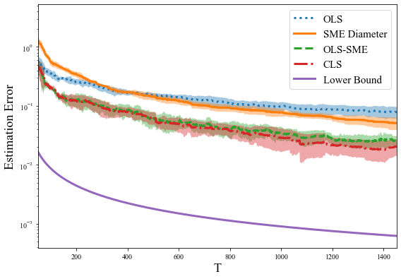
Figure 1: Estimation error convergence for different identification methods

5 conclusion

This work establishes the minimax sample complexity lower bound for system identification under bounded i.i.d. noise, showing that SME-based methods achieve the optimal $\Omega(1/T)$ convergence rate while the ordinary least squares estimator remains limited to $\Omega(1/\sqrt{T})$. Future work includes exploring the dimension dependence of the lower bound and extending the analysis to more general bounded noise models beyond the infinity norm bound.

.1 TV Distance for Scalar Systems

When the noise is bounded, KL divergence between the distributions over state trajectories of two different systems is, in general, infinity. Therefore, we consider total variation (TV) distance to measure how distinguishable state trajectories are when the system has bounded noise. The TV distance is the largest absolute difference between the probabilities that the two probability measures assign to the same event.

Definition 1 (TV Distance).

Consider a measurable space $(\Omega,\mathcal{F})$, where $\Omega$ is a set and $\mathcal{F}$ is a $\sigma$-algebra on $\Omega$. Consider the probability measures $\mathbb{P}$ and $\mathbb{Q}$ defined on $(\Omega,\mathcal{F})$. Assume $\mathbb{P}$ and $\mathbb{Q}$ have the pdfs $p(x)$ and $q(x)$ respectively. The total variation distance between $\mathbb{P}$ and $\mathbb{Q}$ is given by

$$\operatorname{TV}(\mathbb{P},\mathbb{Q}):=\sup_{\mathcal{E}\in\mathcal{F}}|\mathbb{P}(\mathcal{E})-\mathbb{Q}(\mathcal{E})|=\frac{1}{2}\int|p(x)-q(x)|dx.$$

Lemma 1.

Consider two scalar systems $\mathcal{S}_{1}$ and $\mathcal{S}_{2}$ of the form (1) under Assumptions 1-4, where the system parameter is $a_{1}:=\mu+\epsilon$ and $a_{2}:=\mu-\epsilon$, respectively, with $\mu\in(-1+\epsilon,1-\epsilon)$. For $i=1,2$, let $\mathbb{P}_{a_{i}}^{T}$, $f^{T}_{a_{i}}$, and $\mathbb{E}^{T}_{a_{i}}$ denote the probability measure of the state trajectory $\{x_{t}\}^{T}_{t=1}$, the corresponding probability density function, and the expectation with respect to $\mathbb{P}_{a_{i}}^{T}$. Then for small enough $\epsilon>0$, the TV distance between $\mathbb{P}^{T}_{a_{1}}$ and $\mathbb{P}^{T}_{a_{2}}$ satisfies

$$\operatorname{TV}\left(\mathbb{P}^{T}_{a_{1}},\mathbb{P}^{T}_{a_{2}}\right)\leq 2C_{\bar{w}}\epsilon\bar{w}T\frac{1-|\mu|}{(1-|\mu|)^{2}-\epsilon^{2}}.$$ (5)

Proof: For $i=1,2$, let $F_{i}^{T}:=\prod_{t=1}^{T}f_{a_{i}}\left(x_{t}\mid x_{t-1}\right)$.

$$\operatorname{TV}\left(\mathbb{P}^{T}_{a_{1}},\mathbb{P}^{T}_{a_{2}}\right)$$

$$\overset{(a)}{=}\frac{1}{2}\int\dots\int|f_{a_{1}}\left(x_{T}\mid x_{T-1}\right)F_{1}^{T-1}$$

$$\quad\quad-f_{a_{2}}\left(x_{T}\mid x_{T-1}\right)F_{2}^{T-1}|\mathrm{d}x_{T}\mathrm{d}x_{T-1}\dots\mathrm{d}x_{1}$$

$$\overset{(b)}{\leq}\frac{1}{2}\int\dots\int\Big{(}2C_{\bar{w}}\epsilon|x_{T-1}|F_{1}^{T-1}+2C_{\bar{w}}\epsilon|x_{T-1}|F_{2}^{T-1}$$

$$\quad\quad+\left(1-2C_{\bar{w}}\epsilon|x_{T-1}|\right)|F_{1}^{T-1}-F_{2}^{T-1}|\Big{)}\mathrm{d}x_{T-1}\dots\mathrm{d}x_{1}$$

$$=\mathbb{E}_{a_{1}}^{T-1}[C_{\bar{w}}\epsilon|x_{T-1}|]+\mathbb{E}_{a_{2}}^{T-1}[C_{\bar{w}}\epsilon|x_{T-1}|]$$

$$+{\frac{1}{2}}\!\int\dots\int\left(1-2C_{\bar{w}}\epsilon|x_{T-1}|\right)|F_{1}^{T-1}\!-\!F_{2}^{T-1}|\mathrm{d}x_{T-1}\dots\mathrm{d}x_{1}$$

$$\overset{(c)}{\leq}\mathbb{E}_{a_{1}}^{T-1}[C_{\bar{w}}\epsilon|x_{T-1}|]+\mathbb{E}_{a_{2}}^{T-1}[C_{\bar{w}}\epsilon|x_{T-1}|]$$

$$\quad\quad+{\frac{1}{2}}\int\dots\int|F_{1}^{T-1}-F_{2}^{T-1}|\mathrm{d}x_{T-1}\dots\mathrm{d}x_{1}$$

$$=\mathbb{E}_{a_{1}}^{T-1}[C_{\bar{w}}\epsilon|x_{T-1}|]+\mathbb{E}_{a_{2}}^{T-1}[C_{\bar{w}}\epsilon|x_{T-1}|]$$

$$\quad\quad+\operatorname{TV}\left(\mathbb{P}^{T-1}_{a_{1}},\mathbb{P}^{T-1}_{a_{2}}\right)$$

$$\leq C_{\bar{w}}\epsilon\sum_{t=1}^{T-1}\left(\mathbb{E}_{a_{1}}^{t}[|x_{t}|]+\mathbb{E}_{a_{2}}^{t}[|x_{t}|]\right)$$

$$\overset{(d)}{\leq}C_{\bar{w}}\epsilon\bar{w}T\left(\frac{1}{1-|\mu+\epsilon|}+\frac{1}{1-|\mu-\epsilon|}\right)$$

$$\leq 2C_{\bar{w}}\epsilon\bar{w}T\frac{1-|\mu|}{(1-|\mu|)^{2}-\epsilon^{2}},$$

where $(a)$ follows from the definition of TV distance and the Markov property of the LTI system with Assumption 2, as well as Assumption 4. Inequality $(b)$ is due to the following calculation using Assumption 3 and that $f_{a_{i}}(x_{t}|x_{t-1})=f_{w_{t-1}}(x_{t}-a_{i}x_{t-1})$ for $i\in\{1,2\}$:

$$\int|f_{a_{1}}\left(x_{t}\mid x_{t-1}\right)F_{1}^{t-1}-f_{a_{2}}\left(x_{t}\mid x_{t-1}\right)F_{2}^{t-1}|\mathrm{d}x_{t}$$

$$\leq 2C_{\bar{w}}\epsilon|x_{t-1}|F_{1}^{t-1}+2C_{\bar{w}}\epsilon|x_{t-1}|F_{2}^{t-1}$$

$$\quad\quad\quad+\left(1-2C_{\bar{w}}\epsilon|x_{t-1}|\right)|F_{1}^{t-1}-F_{2}^{t-1}|,$$

for all $t\geq 1$. In $(c)$, we use the fact that choosing $\epsilon<\frac{1-\max\{|a_{1}|,|a_{2}|\}}{2C_{\bar{w}}\bar{w}}$ implies that $2C_{\bar{w}}\epsilon|x_{t}|<1$ holds for all $t>1$. Finally, $(d)$ is because for any $a\in\{a_{1},a_{2}\}$.

$$|x_{t}|=\left|\sum^{t-1}_{i=0}a^{t-1-i}w_{i}\right|\leq\sum^{t-1}_{i=0}|a|^{i}|w_{i}|<\frac{\bar{w}}{1-|a|}\,.$$ (6)

$\square$

.2 Proof of Theorem 1

First, we let $\mathbf{v}\in\{+1,-1\}^{n}$ and define the set of matrices $\mathcal{A}_{\epsilon}:=\{\mathbf{A}\in\mathbb{R}^{n\times n}:\mathbf{A}=\mu\mathbf{I}_{n}+\epsilon\operatorname{diag}(\mathbf{v})\}$ with $\epsilon\in(0,1)$, and $\mu\in(-1+\epsilon,1-\epsilon)$. For any estimation procedure that outputs $\hat{\mathbf{A}}_{T}$ as the estimation, define a quantized version $\tilde{\mathbf{A}}_{T}$ as follows:

$$\tilde{A}_{T}{(i,j)}=\begin{cases}0,\quad i\neq j\\ \mu+\epsilon,\quad i=j\;\text{and}\;\hat{A}_{T}{(i,j)}\geq\mu\\ \mu-\epsilon,\quad i=j\;\text{and}\;\hat{A}_{T}{(i,j)}<\mu\end{cases}.$$ (7)

We use $\mathcal{A}_{\epsilon}$ and $\tilde{\mathbf{A}}_{T}$ to lower bound the minimax probability:

$$\inf_{\hat{\mathbf{A}}_{T}}\sup_{\mathbf{A}\in\mathbb{R}^{n\times n}}\mathbb{P}_{\mathbf{A}}^{T}\left(\|\hat{\mathbf{A}}_{T}-\mathbf{A}\|_{2}\geq\epsilon\right)$$ (8)

$$\geq\inf_{\hat{\mathbf{A}}_{T}}\sup_{\mathbf{A}\in\mathcal{A}_{\epsilon}}\mathbb{P}_{\mathbf{A}}^{T}\left(\|\hat{\mathbf{A}}_{T}-\mathbf{A}\|_{2}\geq\epsilon\right)$$

$$\geq\inf_{\tilde{\mathbf{A}}_{T}}\sup_{\mathbf{A}\in\mathcal{A}_{\epsilon}}\mathbb{P}_{\mathbf{A}}^{T}\left(\|\tilde{\mathbf{A}}_{T}-\mathbf{A}\|_{2}\geq 2\epsilon\right).$$

Next, for all $i\in[n]$, we define the events $\mathcal{E}_{1}^{i}:=\{\tilde{A}_{T}{(i,i)}\neq A{(i,i)}\;\text{and}\;\tilde{A}_{T}{(k,k)}=A{(k,k)}\;\text{for}\;k\in[n]\;\text{and}\;k\neq i\}$ and $\mathcal{E}_{2}^{i}:=\{\tilde{A}_{T}{(i,i)}=\mu+\epsilon\;\text{and}\;\tilde{A}_{T}{(k,k)}=A{(k,k)}\;\text{for}\;k\in[n]\;\text{and}\;k\neq i\}$. Let $\mathbf{A}_{\epsilon+}^{(i)}$ denote a fixed matrix from the set $\mathcal{A}_{\epsilon}$ with $A_{\epsilon+}^{(i)}(i,i)=\mu+\epsilon$. Let $\mathbf{A}_{\epsilon-}^{(i)}$ denote the matrix that is equal to $\mathbf{A}_{\epsilon+}^{(i)}$ except that on the $i$th diagonal coordinate, $A_{\epsilon-}^{(i)}(i,i)=\mu-\epsilon$. Clearly, $\|\mathbf{A}_{\epsilon+}^{(i)}-\mathbf{A}_{\epsilon-}^{(i)}\|_{2}=2\epsilon$. Then, we have

$$\inf_{\tilde{\mathbf{A}}_{T}}\sup_{\mathbf{A}\in\mathcal{A}_{\epsilon}}\mathbb{P}_{\mathbf{A}}^{T}\left(\|\tilde{\mathbf{A}}_{T}-\mathbf{A}\|_{2}\geq 2\epsilon\right)$$ (9)

$$=\inf_{\tilde{\mathbf{A}}_{T}}\sup_{\mathbf{A}\in\mathcal{A}_{\epsilon}}\mathbb{P}_{\mathbf{A}}^{T}\left(\|\tilde{\mathbf{A}}_{T}-\mathbf{A}\|_{2}=2\epsilon\right)$$

$$\overset{(a)}{\geq}\inf_{\tilde{\mathbf{A}}_{T}}\sup_{\mathbf{A}\in\mathcal{A}_{\epsilon}}\sum_{i=1}^{n}\mathbb{P}_{\mathbf{A}}^{T}\left(\mathcal{E}^{i}_{1}\right)$$

$$\overset{(b)}{\geq}\frac{1}{2}\inf_{\tilde{\mathbf{A}}_{T}}\sum_{i=1}^{n}\big{[}\mathbb{P}_{\mathbf{A}_{\epsilon+}^{(i)}}^{T}\left(\mathcal{E}^{i}_{1}\right)+\mathbb{P}_{\mathbf{A}_{\epsilon-}^{(i)}}^{T}\left(\mathcal{E}^{i}_{1}\right)\big{]}$$

$$\overset{(c)}{=}\frac{1}{2}\inf_{\tilde{\mathbf{A}}_{T}}\sum_{i=1}^{n}\big{[}1-\big{(}\mathbb{P}_{\mathbf{A}_{\epsilon+}^{(i)}}^{T}\left(\mathcal{E}^{i}_{2}\right)-\mathbb{P}_{\mathbf{A}_{\epsilon-}^{(i)}}^{T}\left(\mathcal{E}^{i}_{2}\right)\big{)}\big{]}$$

$${\geq}\frac{1}{2}\inf_{\tilde{\mathbf{A}}_{T}}\sum_{i=1}^{n}\big{[}1-\big{|}\mathbb{P}_{\mathbf{A}_{\epsilon+}^{(i)}}^{T}\left(\mathcal{E}^{i}_{2}\right)-\mathbb{P}_{\mathbf{A}_{\epsilon-}^{(i)}}^{T}\left(\mathcal{E}^{i}_{2}\right)\big{|}\big{]}$$

$$\overset{(d)}{\geq}\frac{1}{2}\inf_{\tilde{\mathbf{A}}_{T}}\sum_{i=1}^{n}\big{[}1-\operatorname{TV}\big{(}\mathbb{P}_{\mathbf{A}_{\epsilon+}^{(i)}}^{T},\mathbb{P}_{\mathbf{A}_{\epsilon-}^{(i)}}^{T}\big{)}\big{]}$$

$$\overset{(e)}{\geq}\frac{1}{2}n\left(1-\operatorname{TV}\left(\mathbb{P}^{T}_{a_{1}},\mathbb{P}^{T}_{a_{2}}\right)\right),$$

where $(a)$ is because $\{\mathcal{E}_{1}^{i}\}_{i=1}^{n}$ are $n$ disjoint events and $\cup_{i=1}^{n}\mathcal{E}_{1}^{i}\subseteq\{\|\tilde{\mathbf{A}}_{T}-\mathbf{A}\|_{2}=2\epsilon\}$. In $(b)$, we use the average of two points $\mathbf{A}^{i}_{\epsilon+}$ and $\mathbf{A}^{i}_{\epsilon-}$ to lower bound the supremum over all $\mathcal{A}_{\epsilon}$, whereas $(c)$ is based on the facts that $\mathbb{P}_{\mathbf{A}_{\epsilon+}^{(i)}}^{T}\left(\mathcal{E}^{i}_{1}\right)=1-\mathbb{P}_{\mathbf{A}_{\epsilon+}^{(i)}}^{T}\left(\mathcal{E}^{i}_{2}\right)$ and $\mathbb{P}_{\mathbf{A}_{\epsilon-}^{(i)}}^{T}\left(\mathcal{E}^{i}_{1}\right)=\mathbb{P}_{\mathbf{A}_{\epsilon-}^{(i)}}^{T}\left(\mathcal{E}^{i}_{2}\right)$. Inequality $(d)$ is based on Definition 1 for the TV distance, and $(e)$ is from the noise coordinate independence condition in Assumption 2 with $a_{1}=\mu+\epsilon$ and $a_{2}=\mu-\epsilon$. Finally, by Lemma 1 with $\mu=0$, we have

$$\inf_{\hat{\mathbf{A}}_{T}}\sup_{\mathbf{A}\in\mathbb{R}^{n\times n}}\mathbb{P}^{T}_{\mathbf{A}}\left(\|\hat{\mathbf{A}}_{T}-\mathbf{A}\|_{2}\geq\epsilon\right)$$ (10)

$$\geq\frac{1}{2}n\left(1-2C_{\bar{w}}\epsilon\bar{w}T\frac{1}{1-\epsilon^{2}}\right)\overset{(a)}{\geq}\frac{1}{2}n\left(1-4C_{\bar{w}}\epsilon\bar{w}T\right).$$

where $(a)$ is by making $\epsilon$ small enough and in particular $\epsilon^{2}<\frac{1}{2}$. Choosing $\delta$ less than RHS of the second inequality in (10) completes the proof. $\square$

.3 Proof of Theorem 2

The proof leverages the following quantitative description of the central limit theorem for self-normalized martingales applied to OLS for data from a single trajectory.

Lemma 2 (Berry–Esseen for Self-Normalized Martingale for OLS,[25, Theorem 3.2]).

Consider the system in (1) with a scalar system parameter $a$ and i.i.d noise $w_{t}$ and data $\{x_{t}\}_{t=1}^{T}$ from a single trajectory. Suppose that $\mathbb{E}[|w_{t}|^{4}]<\infty$ and $\mathbb{E}\left[w_{t}^{2}\right]=\sigma_{w}^{2}$ with $\sigma_{w}>0$. Then there exists a positive universal constant $C_{1}$ such that for all $\beta\in\mathbb{R}$,

$$\sup_{\beta\in\mathbb{R}}\left|\mathbb{P}\left(\left(\widehat{a}^{\textsf{OLS}}_{T}-a\right)\sqrt{\sum_{t=1}^{T}x_{t}^{2}}\leq\beta\sigma_{w}\right)-\Phi(\beta)\right|$$ (11)

$$\leq C_{1}\Biggl{(}T^{-1}\left(\frac{1}{(1-a^{2})^{2}}+\frac{1}{1-a^{4}}\frac{\mathbb{E}\left[|w_{t}|^{4}\right]}{\sigma_{w}^{4}}\right)$$

$$\quad\quad\quad\quad+\underbrace{\frac{\mathbb{E}\left[\left(\sum_{t=1}^{T}(x_{t}^{2}-\mathbb{E}[x_{t}^{2}])\right)^{2}\right]}{\left(\sum_{t=1}^{T}\mathbb{E}[x_{t}^{2}]\right)^{2}}}_{\mathbb{T}}\Biggr{)}^{1/5},$$

where the probability $\mathbb{P}$ is with respect to the randomness of $\{w_{t}\}_{t=0}^{T-1}$ and $\Phi(\epsilon)$ is the standard Gaussian cumulative distribution function.

In what follows, we use the bound (11) to show that the probability of the estimation error being less than a fixed number $\epsilon$ is upper bounded by $O(1/\sqrt{T})$. We will do so by bounding key quantities in (11). In particular, we first upper bound the numerator and lower bound the denominator of $\mathbb{T}$. Then, we upper bound $\sqrt{\sum_{t=1}^{T}x_{t}^{2}}$ with high probability in the LHS of (11). Taking the intersection of the events that $\sqrt{\sum_{t=1}^{T}x_{t}^{2}}$ is small and $(\widehat{a}^{\textsf{OLS}}_{T}-a)$ is small, we arrive at the final conclusion.

Step 1: Bounding terms in $\mathbb{T}$. We will first provide an upper bound to the numerator in the following lemma.

Lemma 3.

Consider the scalar system (1) under Assumption 2 with a single state trajectory $\{x_{t}\}_{t=1}^{T}$. Then,

$$\mathbb{E}\left[\left(\sum_{t=1}^{T}\left(x_{t}^{2}-\mathbb{E}[x_{t}^{2}]\right)\right)^{2}\right]\leq\frac{\bar{w}^{4}(1+a^{2})}{(1-a)^{4}(1-a^{2})}T.$$

Proof: For $s>t$, define $\tilde{x}_{s,t}:=\sum_{j=t}^{s-1}a^{s-1-j}w_{j}$ which is independent of $x_{t}$. Then $\mathbb{E}[\tilde{x}_{s,t}]=0$ and $x_{s}^{2}$ can be represented as

$$x_{s}^{2}=(a^{s-t}x_{t}+\tilde{x}_{s,t})^{2}=a^{2(s-t)}x_{t}^{2}+2a^{s-t}x_{t}\tilde{x}_{s,t}+\tilde{x}_{s,t}^{2}.$$ (12)

Let $\operatorname{Cov}$ and $\operatorname{Var}$ denote the covariance and the variance respectively. The covariance between $x_{t}^{2}$ and $x_{s}^{2}$ is

$$\operatorname{Cov}(x_{t}^{2},x_{s}^{2})$$ (13)

$$\overset{(a)}{=}\operatorname{Cov}\Bigl{(}x_{t}^{2},\;a^{2(s-t)}x_{t}^{2}+2a^{s-t}x_{t}\,\tilde{x}_{s,t}+\tilde{x}_{s,t}^{2}\Bigr{)}$$

$$\overset{(b)}{\geq}a^{2(s-t)}\,\operatorname{Cov}(x_{t}^{2},x_{t}^{2})+2a^{s-t}\,\operatorname{Cov}(x_{t}^{2},x_{t}\,\tilde{x}_{s,t})$$

$$\quad\quad\quad\quad\quad\quad\quad\quad\quad\quad\,\,\quad\quad\quad+\operatorname{Cov}(x_{t}^{2},\tilde{x}_{s,t}^{2})$$

$$\overset{(c)}{\geq}a^{2(s-t)}\,\operatorname{Var}(x_{t}^{2}),$$

where $(a)$ is based on (12), $(b)$ is from the linearity of covariance, and $(c)$ is because $\operatorname{Cov}(x_{t}^{2},x_{t}\,\tilde{x}_{s,t})=\mathbb{E}\left[x_{t}^{3}\tilde{x}_{s,t}\right]-\mathbb{E}\left[x_{t}^{2}\right]\mathbb{E}\left[x_{t}\tilde{x}_{s,t}\right]=0$ and $\operatorname{Cov}(x_{t}^{2},\tilde{x}_{s,t}^{2})=\mathbb{E}\left[x_{t}^{2}\tilde{x}_{s,t}^{2}\right]-\mathbb{E}\left[x_{t}^{2}\right]\mathbb{E}\left[\tilde{x}_{s,t}^{2}\right]=0.$

Therefore,

$$\mathbb{E} \left[\left(\sum_{t=1}^{T}\left(x_{t}^{2}-\mathbb{E}[x_{t}^{2}]\right)\right)^{2}\right]$$

$$=\sum_{t=1}^{T}\operatorname{Var}(x_{t}^{2})+2\sum_{t=1}^{T-1}\sum_{k=1}^{T-t}\operatorname{Cov}(x_{t}^{2},x_{t+k}^{2})$$

$$\overset{(a)}{\leq}\sum_{t=1}^{T}\operatorname{Var}(x_{t}^{2})+2\sum_{t=1}^{T-1}\sum_{k=1}^{T-t}a^{2k}\,\operatorname{Var}(x_{t}^{2})$$

$$\overset{(b)}{\leq}\sum_{t=1}^{T}\frac{\bar{w}^{4}}{(1-|a|)^{4}}+2\sum_{t=1}^{T-1}\sum_{k=1}^{T-t}a^{2k}\frac{\bar{w}^{4}}{(1-|a|)^{4}}$$

$$\leq\frac{\bar{w}^{4}}{(1-|a|)^{4}}\sum_{t=1}^{T}\left(1+2\sum^{\infty}_{k=1}a^{2k}\right)$$

$$\leq\frac{\bar{w}^{4}}{(1-|a|)^{4}}\left(1+\frac{2a^{2}}{1-a^{2}}\right)T,$$

where $(a)$ is from (13) and $(b)$ is because $\operatorname{Var}(x_{t}^{2})=\mathbb{E}[(x_{t}^{2}-\mathbb{E}[x_{t}^{2}])^{2}]\leq\mathbb{E}[x_{t}^{4}]<\frac{\bar{w}^{4}}{(1-|a|)^{4}}$, for which the last inequality is based on (6). $\square$

Next, we will find a lower bound for the denominator of $\mathbb{T}$, where

$$\mathbb{E}\left[x_{t}^{2}\right] =\mathbb{E}\left[\left(\sum^{t-1}_{i=0}a^{t-1-i}w_{i}\right)^{2}\right]$$ (14)

$$=\sum^{t-1}_{i=0}a^{2(t-1-i)}\mathbb{E}\left[w_{i}^{2}\right]\geq\mathbb{E}\left[w_{t}^{2}\right]=\sigma_{w}^{2}.$$

Step 2: Bounding $\sqrt{\sum_{t=1}^{T}x_{t}^{2}}$ with high probability.

Lemma 4 ([6, Theorem 2]).

Consider the system (1) with a scalar system parameter $a$ and i.i.d sub-Gaussian noise $w_{t}$ and a single trajectory $\{x_{t}\}_{t=1}^{T}$. Let $\varepsilon>0$. Then, for some universal constants $C_{2},C_{3}>0$, we have that with probability at least $1-2\exp\left(-C_{2}\gamma^{2}\frac{(1-|a|)^{2}}{\left(\sum_{s=0}^{T-1}\sum_{k=0}^{s}|a|^{2k}\right)}+C_{3}\right),$

$$\left(1-K^{2}\gamma\right)\sqrt{\sum_{s=0}^{T-1}\sum_{k=0}^{s}|a|^{2k}}$$

$$\leq\sqrt{\sum_{t=1}^{T}x_{t}^{2}}\leq\left(1+K^{2}\gamma\right)\sqrt{\sum_{s=0}^{T-1}\sum_{k=0}^{s}|a|^{2k}},$$

where $\gamma\in(0,\frac{1}{K^{2}})$ and $K$ is an upper bound of the sub-Gaussian norm of $w_{t}$, e.g., $K\geq\|w_{t}\|_{\psi_{2}}$, with $\|w_{t}\|_{\psi_{2}}:=\inf\left\{\kappa>0:\mathbb{E}\left[\exp(w_{t}^{2}/\kappa^{2})\right]\leq 2\right\}$.

Note that any bounded random variable $X$ is sub-Gaussian with $\|X\|_{\psi_{2}}\leq\frac{\|X\|_{\infty}}{\sqrt{\ln 2}}$ [26]. Therefore, considering Lemma 4 with $K=\frac{(1-a^{T-1})\bar{w}}{(1-|a|)\sqrt{\ln 2}}<\frac{\bar{w}}{(1-|a|)\sqrt{\ln 2}}$ and $\gamma=\frac{1}{2K^{2}}$, it can be seen that

$$\quad\quad\mathbb{P} \left(\frac{1}{\sqrt{\sum_{t=1}^{T}x_{t}^{2}}}\leq\frac{2}{\sqrt{T}}\right)$$ (15)

$$\quad\leq 2\exp\left(-C_{2}\gamma^{2}\frac{(1-|a|)^{2}}{\left(\sum_{s=0}^{T-1}\sum_{k=0}^{s}a^{2k}\right)}+C_{3}\right)$$

$$\quad\overset{(a)}{\leq}C_{5}\exp\left(-C_{2}\frac{(1-|a|)^{4}(1-a^{2})}{2\bar{w}^{2}T\ln 2}\right),$$

where $C_{5}:=2\exp(C_{3})$ and $(a)$ is because $\sum_{k=0}^{s}a^{2k}\leq\frac{1}{1-a^{2}}$ for all $s\geq 0$ and $a^{2}<1$.

Step 3: Final bound.

We are now in a position to revisit Lemma 2. Consider (11) and plug in $\beta=\epsilon\sqrt{T}$, we get

$$\mathbb{P}\left(|\widehat{a}^{\textsf{OLS}}_{T}-a|\sqrt{\sum_{t=1}^{T}x_{t}^{2}}\leq\epsilon\sqrt{T}\sigma_{w}\right)$$

$$\leq\Phi(\epsilon\sqrt{T})+C_{1}\Bigg{(}\left(\frac{1}{\left(1-a^{2}\right)^{2}}+\frac{1}{1-a^{4}}\frac{\mathbb{E}\left[\left|w_{t}\right|^{4}\right]}{\sigma_{w}^{4}}\right)T^{-1}$$

$$\,\,\,\quad\quad\quad\quad\quad\quad\quad\quad\quad\quad+\frac{\mathbb{E}\left[\left|\sum_{t=1}^{T}\left(x_{t}^{2}-\mathbb{E}[x_{t}^{2}]\right)\right|^{2}\right]}{\left(\sum_{t=1}^{T}\mathbb{E}[x_{t}^{2}]\right)^{2}}\Bigg{)}^{1/5}$$

$$\overset{(a)}{\leq}\Phi(\epsilon\sqrt{T})+C_{1}\Bigg{(}\left(\frac{1}{\left(1-a^{2}\right)^{2}}+\frac{1}{1-a^{4}}\frac{\bar{w}^{4}}{\sigma_{w}^{4}}\right)T^{-1}$$

$$\quad\quad\quad\quad\quad\quad\quad\quad\quad\quad\quad\quad\quad\quad\quad+\frac{\frac{\bar{w}^{4}(1+a^{2})}{(1-|a|)^{4}(1-a^{2})}T}{\left(\sigma_{w}^{2}T\right)^{2}}\Bigg{)}^{1/5}$$

$$\overset{(b)}{\leq}\sqrt{\frac{2}{\pi}}\epsilon\sqrt{T}+C_{4}T^{-\frac{1}{5}},$$ (16)

where

$$C_{4}\!\!:=\!\!C_{1}\!\!\left(\!\frac{1}{\left(\!1-a^{2}\right)^{2}}\!+\!\frac{\bar{w}^{4}}{(1-a^{4})\sigma_{w}^{4}}\!+\!\frac{\bar{w}^{4}(1+a^{2})}{(1-|a|)^{4}(1-a^{2})\sigma_{w}^{4}}\!\right)^{1/5}\!\!\!\!,$$

$(a)$ is implied by (6), (14), and Lemma 3, while $(b)$ is based on the fact that for a standard Gaussian random variable $g$, for any $u\in\mathbb{R}$ and $t>0$, $\mathbb{P}(|g-u|<t)<\sqrt{\frac{2}{\pi}}t$.

Finally, combining (15) and (16) and taking the intersection of both events, we have that for all $T\geq 1$, $\mathbb{P}_{a}^{T}\left(|\widehat{a}^{\textsf{OLS}}_{T}-a|\leq\epsilon\right)\leq$

$$\min\!\bigg{\{}\!\frac{1}{\sqrt{2\pi}\sigma_{w}}\epsilon\sqrt{T}+\frac{C_{4}}{T^{1/5}},C_{5}\exp\left(\frac{-C_{2}(1-a)^{4}(1-a^{2})}{2\bar{w}^{2}T\ln 2}\!\right)\!\!\bigg{\}}.$$

Making $\epsilon>0$ small enough and choosing $1-\delta$ bigger than the right-hand side of the above inequality completes the proof. $\square$

References

• [1] M. Simchowitz, H. Mania, S. Tu, M. I. Jordan, and B. Recht, “Learning without mixing: Towards a sharp analysis of linear system identification,” in Conference On Learning Theory. PMLR, 2018, pp. 439–473.
• [2] S. Oymak and N. Ozay, “Non-asymptotic identification of lti systems from a single trajectory,” in 2019 American control conference (ACC). IEEE, 2019, pp. 5655–5661.
• [3] Y. Li, J. Yu, L. Conger, T. Kargin, and A. Wierman, “Learning the uncertainty sets of linear control systems via set membership: A non-asymptotic analysis,” in Forty-first International Conference on Machine Learning, 2024.
• [4] D. Foster, T. Sarkar, and A. Rakhlin, “Learning nonlinear dynamical systems from a single trajectory,” in Learning for Dynamics and Control. PMLR, 2020, pp. 851–861.
• [5] Y. Sattar, S. Oymak, and N. Ozay, “Finite sample identification of bilinear dynamical systems,” in 2022 IEEE 61st Conference on Decision and Control (CDC). IEEE, 2022, pp. 6705–6711.
• [6] Y. Jedra and A. Proutiere, “Finite-time identification of stable linear systems optimality of the least-squares estimator,” in 2020 59th IEEE Conference on Decision and Control (CDC). IEEE, 2020, pp. 996–1001.
• [7] S. Dean, H. Mania, N. Matni, B. Recht, and S. Tu, “On the sample complexity of the linear quadratic regulator,” Foundations of Computational Mathematics, vol. 20, no. 4, pp. 633–679, 2020.
• [8] M. Simchowitz and D. Foster, “Naive exploration is optimal for online lqr,” in International Conference on Machine Learning. PMLR, 2020, pp. 8937–8948.
• [9] T. Kargin, S. Lale, K. Azizzadenesheli, A. Anandkumar, and B. Hassibi, “Thompson sampling achieves $\tilde{o}\sqrt{t}$ regret in linear quadratic control,” in Conference on Learning Theory. PMLR, 2022, pp. 3235–3284.
• [10] S. Lale, K. Azizzadenesheli, B. Hassibi, and A. Anandkumar, “Reinforcement learning with fast stabilization in linear dynamical systems,” in International Conference on Artificial Intelligence and Statistics. PMLR, 2022, pp. 5354–5390.
• [11] H. Zhou and V. Tzoumas, “Simultaneous system identification and model predictive control with no dynamic regret,” arXiv preprint arXiv:2407.04143, 2024.
• [12] E.-W. Bai, H. Cho, and R. Tempo, “Convergence properties of the membership set,” Automatica, vol. 34, no. 10, pp. 1245–1249, 1998.
• [13] H. Akçay, “The size of the membership-set in a probabilistic framework,” Automatica, vol. 40, no. 2, pp. 253–260, 2004.
• [14] W. Kitamura, Y. Fujisaki, and E.-W. Bai, “The size of the membership set in the presence of disturbance and parameter uncertainty,” in Proceedings of the 44th IEEE Conference on Decision and Control. IEEE, 2005, pp. 5698–5703.
• [15] E.-W. Bai, R. Tempo, and H. Cho, “Membership set estimators: size, optimal inputs, complexity and relations with least squares,” IEEE Transactions on Circuits and Systems I: Fundamental Theory and Applications, vol. 42, no. 5, pp. 266–277, 1995.
• [16] P. Hespanhol and A. Aswani, “Statistical consistency of set-membership estimator for linear systems,” IEEE Control Systems Letters, vol. 4, no. 3, pp. 668–673, 2020.
• [17] P. C. Phillips and T. Magdalinos, “Inconsistent var regression with common explosive roots,” Econometric Theory, vol. 29, no. 4, pp. 808–837, 2013.
• [18] T. Sarkar and A. Rakhlin, “Near optimal finite time identification of arbitrary linear dynamical systems,” in International Conference on Machine Learning. PMLR, 2019, pp. 5610–5618.
• [19] M. J. Wainwright, High-dimensional statistics: A non-asymptotic viewpoint. Cambridge university press, 2019, vol. 48.
• [20] J. Mourtada, “Exact minimax risk for linear least squares, and the lower tail of sample covariance matrices,” The Annals of Statistics, vol. 50, no. 4, pp. 2157–2178, 2022.
• [21] Y. Yi and M. Neykov, “Non-asymptotic bounds for the $l_{\infty}$ estimator in linear regression with uniform noise,” Bernoulli, vol. 30, no. 1, pp. 534–553, 2024.
• [22] M. Rudelson and R. Vershynin, “The littlewood–offord problem and invertibility of random matrices,” Advances in Mathematics, vol. 218, no. 2, pp. 600–633, 2008.
• [23] Y. Jedra and A. Proutiere, “Sample complexity lower bounds for linear system identification,” in 2019 IEEE 58th Conference on Decision and Control (CDC). IEEE, 2019, pp. 2676–2681.
• [24] S. Tu, R. Frostig, and M. Soltanolkotabi, “Learning from many trajectories,” Journal of Machine Learning Research, vol. 25, no. 216, pp. 1–109, 2024.
• [25] X. Fan and Q.-M. Shao, “Berry–esseen bounds for self-normalized martingales,” Communications in Mathematics and Statistics, vol. 6, no. 1, pp. 13–27, 2018.
• [26] R. Vershynin, High-dimensional probability: An introduction with applications in data science. Cambridge university press, 2018, vol. 47.