Modeling and forecasting subnational age distribution of death counts

Abstract

This paper presents several forecasting methods to model and forecast subnational age distribution of death counts. The age distribution of death counts has many similarities to probability density functions, which are nonnegative and have a constrained integral, and thus live in a constrained nonlinear space. To address the nonlinear nature of objects, we implement a cumulative distribution function transformation that has an additional monotonicity. Using the Japanese subnational life-table death counts obtained from the Japanese Mortality Database (2025), we evaluate the forecast accuracy of the transformation and forecasting methods. The improved forecast accuracy of life-table death counts implemented here will be of great interest to demographers in estimating regional age-specific survival probabilities and life expectancy.

Keywords: constrained functional time series; cumulative distribution function transformation; (split) conformal prediction; life-table death counts; principal component analysis

1 Introduction

Density-valued objects for multiple groups are common, with examples including income distributions across different populations (Kneip & Utikal, 2001), financial return distributions for multiple stocks (Petersen et al., 2022), distributions of bidding times in online auctions for various items (Wang et al., 2008), and subnational age distributions of deaths in demography (Jiménez-Varón et al., 2025), among others. We present several forecasting methods to model and predict the subnational age distribution of deaths, which are also useful for applications in actuarial science, such as fixed-term or lifetime annuity pricing.

Since age distributions of deaths naturally take the form of density functions, they are well-suited for modeling using advanced forecasting techniques from compositional and functional data analyses. Oeppen (2008) demonstrates that using compositional data analysis to forecast the age distribution of death counts performs similarly in accuracy to forecasting age-specific mortality rates. Within the compositional data analysis, the Lee-Carter model is frequently applied to model and forecast unconstrained data. Shang & Haberman (2020) extend this approach by incorporating a functional data analytic perspective, which includes multiple principal components and nonparametric smoothing. Recently, Shang & Haberman (2025) introduce a cumulative distribution function (CDF) transformation, converting each year’s age distribution of deaths into a probability bounded within the unit interval to address the presence of zero values. Through cumulative summation, a probability density function can be transformed into a CDF, which provides the additional benefit of monotonicity (see also Mayhew & Smith, 2013). With a time series of CDFs, it is common to model and extrapolate its pattern via a logistic transformation.

Multiple density-valued objects are observed over time are related to high-dimensional functional time series (HDFTS). In the statistical literature, Zhou & Dette (2023) derive Gaussian and multiplier bootstrap approximations for sums of HDFTS. With these approximations, they construct joint simultaneous confidence bands for the mean functions and develop a hypothesis to test whether the mean functions in the cross-sectional dimension exhibit parallel behavior. Hallin et al. (2023) investigate the representation of HDFTS using a factor model, determining conditions on the eigenvalues of the covariance operator crucial for establishing the existence and uniqueness of the factor model. Gao et al. (2019) adopt a two-stage approach, combining truncated principal component analysis and a separate scalar factor model for the resulting panels of scores. Tavakoli et al. (2023) introduce a functional factor model with a functional factor loading and a vector of real-valued factors, while Guo et al. (2024) propose a functional factor model with a real-valued factor loading and a functional factor. Leng et al. (2024) introduce a unified framework that accommodates both types of factor models. Tang et al. (2022) study clustering for age-specific subnational mortality rates, which is an example of HDFTS. Li et al. (2024) introduce hypothesis tests and estimation procedures for testing and locating (common) change points. Chang et al. (2025) develop a two-stage procedure for modeling and forecasting HDFTS.

Our contributions are twofold. First, we present several visualization techniques to capture the patterns in age distribution of death counts and display contrasts between subnational and national data. Second, we revisit several forecasting methods and compare their point and interval forecast accuracy with applications to subnational life-table death counts.

Our paper is structured as follows. In Section 2, we describe our motivating data set and introduce a series of image plots for displaying important features in HDFTS. In Section 3, we present the CDF transformations. Within the CDF transformation, we consider a number of forecasting methods in Section 4 to model and forecast unconstrained functional time-series data. In Section 5, we propose two general strategies for constructing pointwise prediction intervals for the age distribution of death counts. In Section 6, we evaluate and compare point forecast accuracy using the Kullback-Leibler divergence (KLD) and Jensen-Shannon divergence (JSD), and interval forecast accuracy using the coverage probability difference (CPD) and interval score. Section 7 concludes with some ideas on how the methodology presented can be further extended.

2 Subnational age distribution of death in Japan

In many developed countries such as Japan, increases in longevity and an aging population have led to concerns about the sustainability of pensions, health, and aged care systems (see, e.g., Coulmas, 2007). These concerns have resulted in a surge of interest among government policy makers in accurately modeling and forecasting age-specific mortality. Subnational forecasts of age-specific mortality are useful for informing policy within local regions and any improvement in forecast accuracy of mortality is beneficial for determining the allocation of current and future resources at the national and subnational levels.

In demography, the age distribution of deaths provides important insights into longevity and lifespan variability that cannot be grasped directly from the central mortality rate or survival function. As pointed out by Oeppen (2008), the age distribution of death counts is more suitable than central mortality rates for computing life expectancy and annuity premia. In addition to providing an informative description of the mortality experience of a population, life-table death counts yield readily available information on the “central longevity indicators” (e.g., mean, median, and modal age at death, see Cheung et al., 2005; Canudas-Romo, 2010) and lifespan variability (e.g., van Raalte & Caswell, 2013; Aburto & van Raalte, 2018).

We study Japanese lifetable death counts from 1975 to 2022, obtained from the Japanese Mortality Database (2025). We consider ages from 0 to 110 in single years of age. Figure 1 shows rainbow plots of the female and male age-specific life-table death counts in Japan from 1975 to 2022. The time ordering of the curves follows the color order of a rainbow, where curves from the distant past are shown in red and the more recent curves are shown in violet. The figures show typical mortality curves for a developed country, with a decreasing trend in infant death counts. A typical negatively skewed distribution for the life-table death counts is apparent where the peaks shift to higher ages for both females and males. This shift is a main source of longevity risk, which is a major issue for insurers and pension funds, especially in the selling and risk management of annuity products (see Denuit et al., 2007, for a discussion). Moreover, the spread of the distribution indicates lifespan variability. A decrease in variability over time can be observed directly and can be measured by the Gini coefficient (Wilmoth & Horiuchi, 1999; Debón et al., 2017).

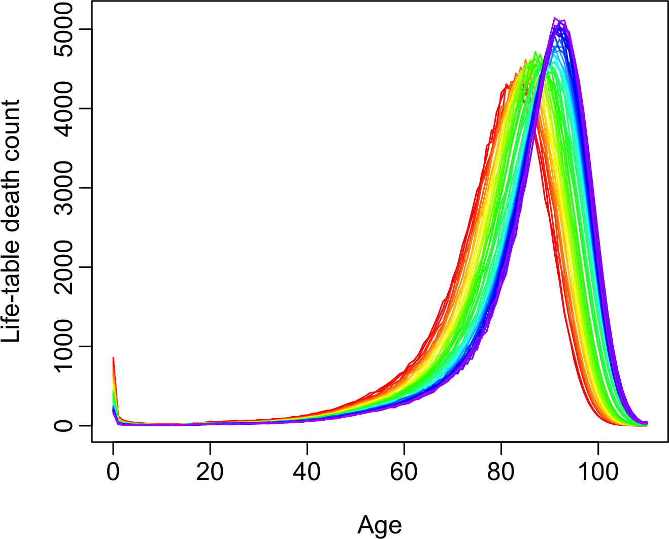
(a) Japanese female data

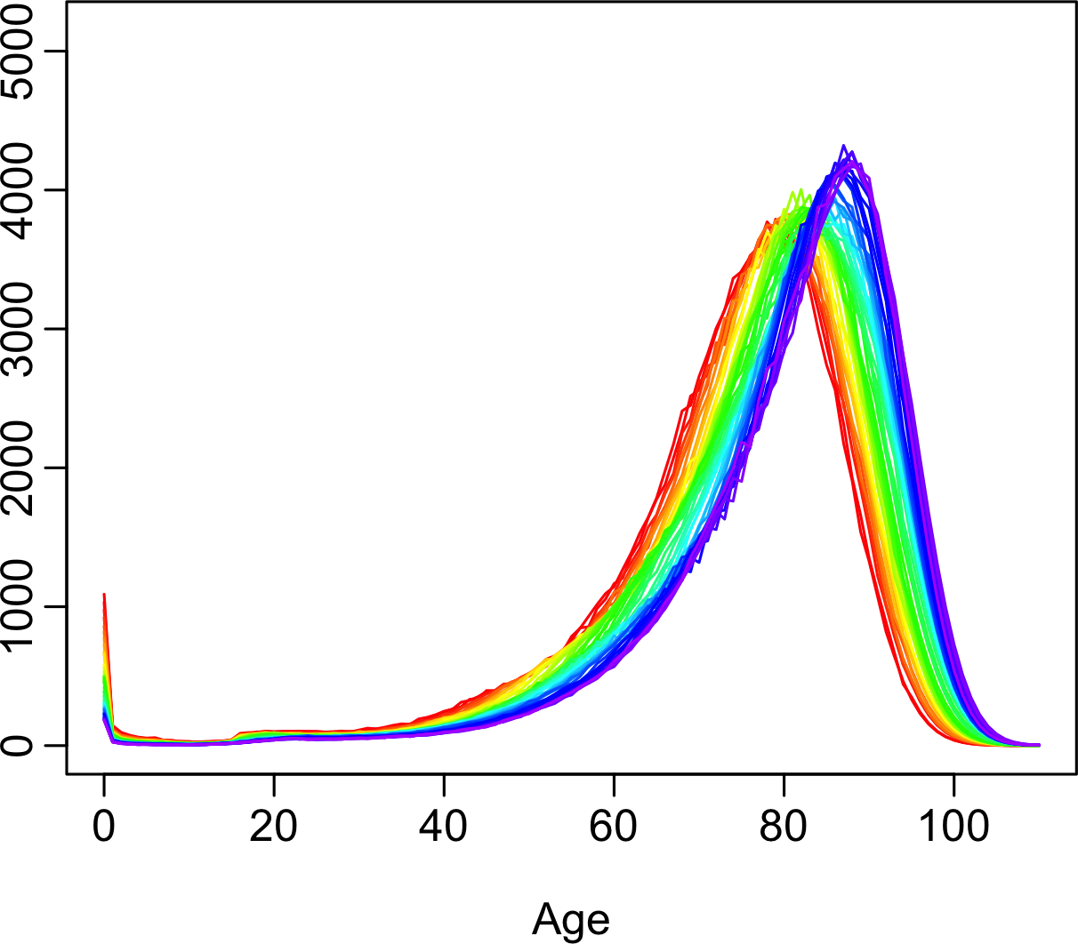
(b) Japanese male data

Figure 1: Functional time series graphical displays of age-specific life-table death counts from 1975 to 2022 in a single-year group. The oldest years are shown in red, with the most recent years in violet. Curves are ordered chronologically according to the colors of the rainbow.

2.1 Image plots

Another visual perspective of the data is shown in the image plot of Figure 2. Here, we graph the symmetric KLD between life-table death counts for each prefecture to life-table death counts for the whole country, thus allowing relative mortality comparisons to be made. A divergent color palette is used with red representing larger KLD values (i.e., greater difference between subnational and national data) and yellow denoting smaller KLD values. The prefectures are ordered geographically from north to south, so the most northerly prefecture (Hokkaido) is at the top of the panels, and the most southerly prefecture (Okinawa) is at the bottom.

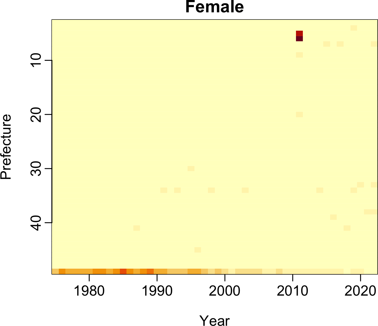
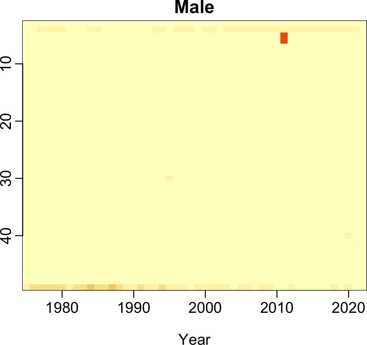
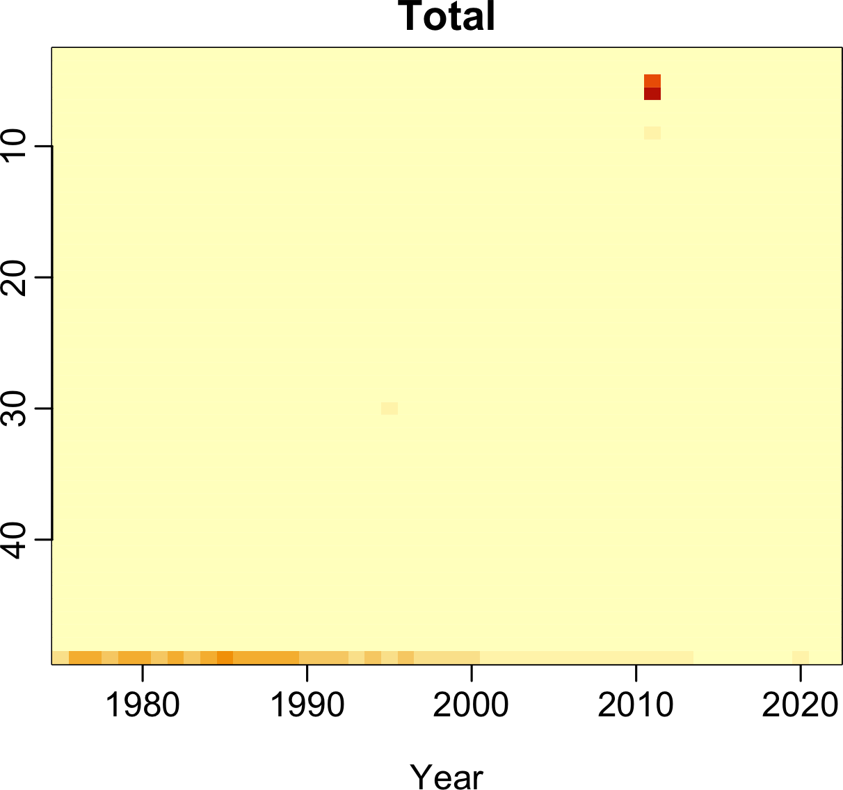
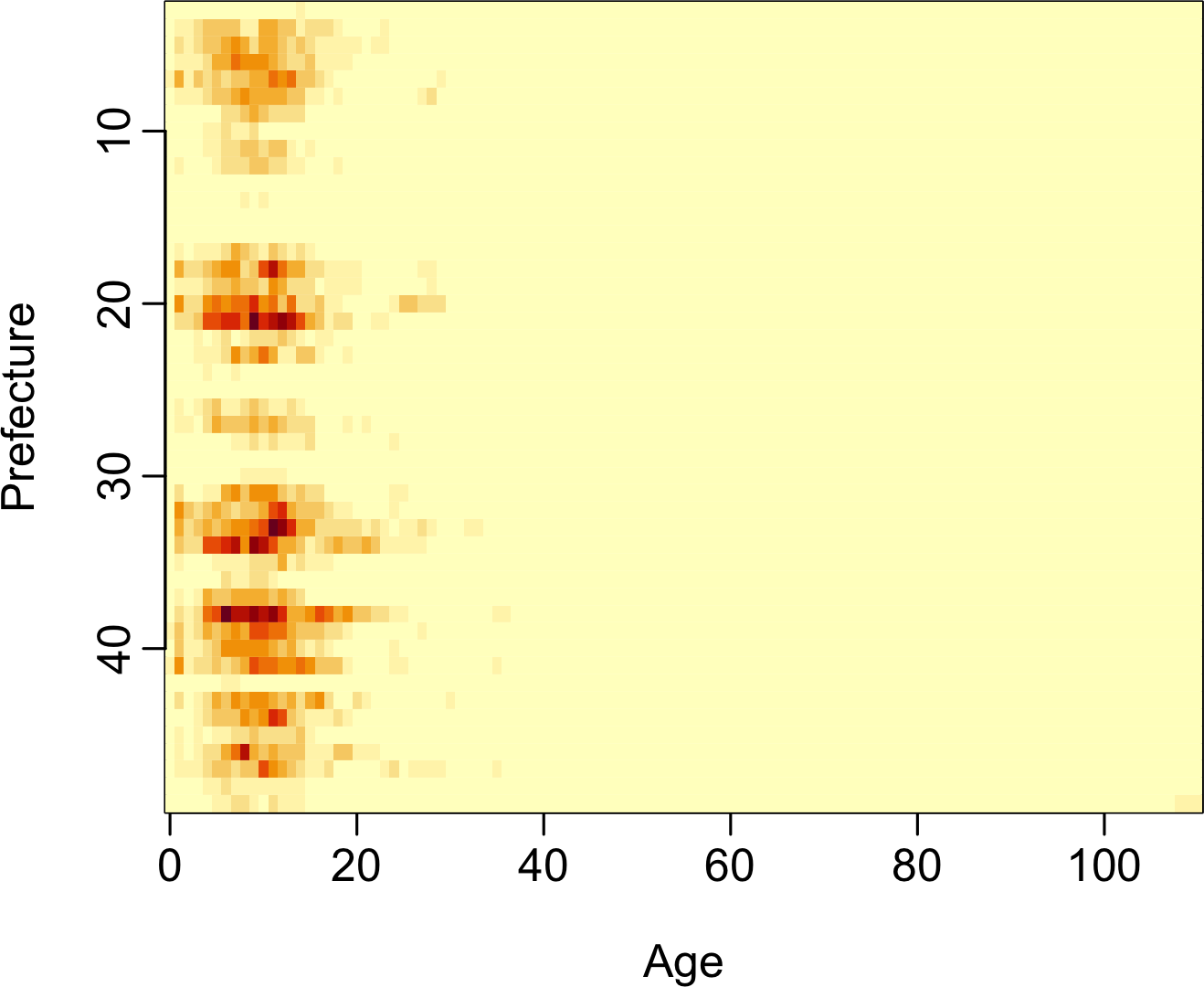
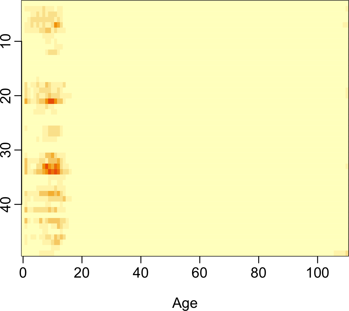
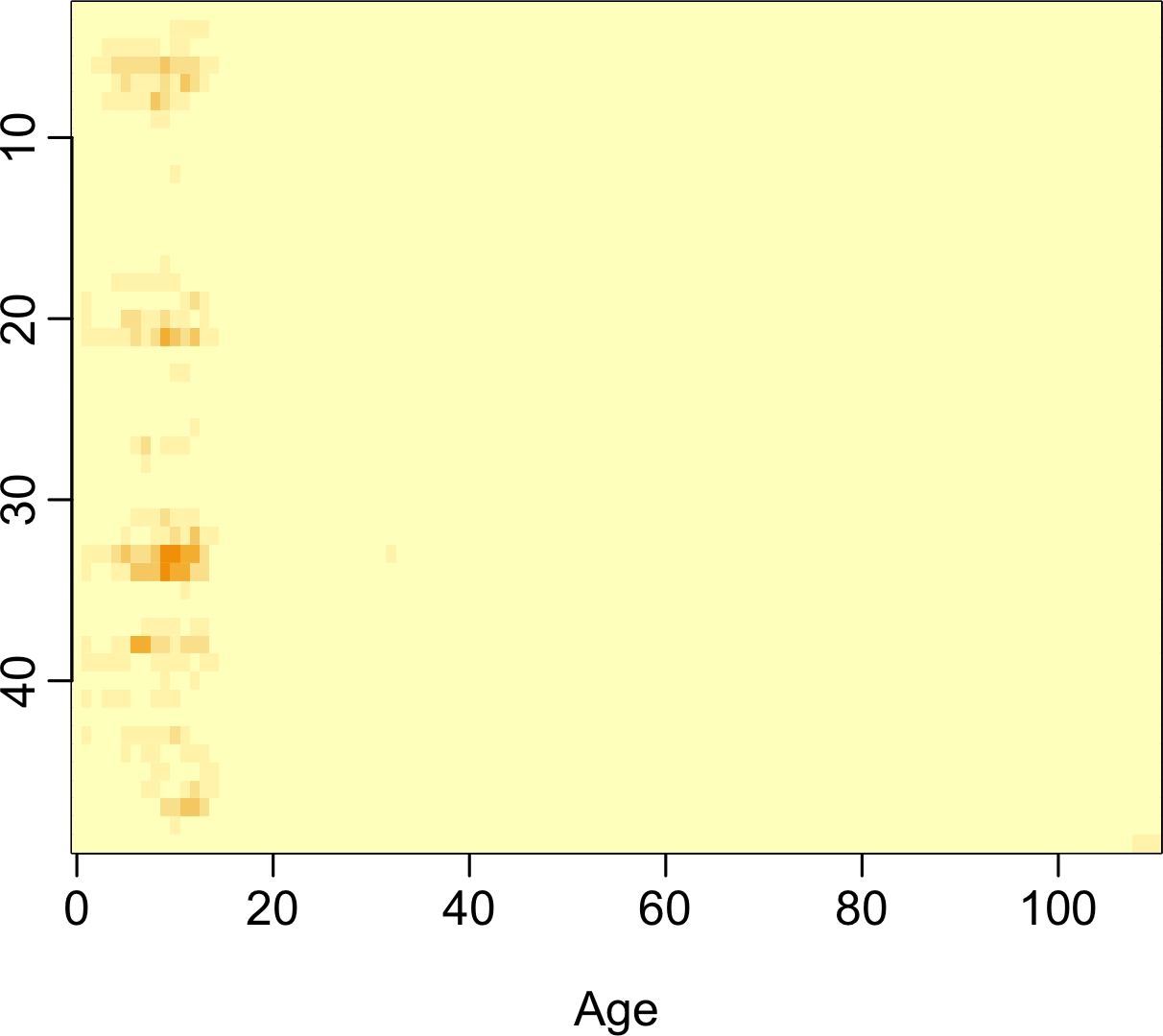
Figure 2: Image plots showing the symmetric KLD introduced in (9) between life-table death counts of a prefecture and life-table death counts of the whole country. The top panel shows mortality averaged over ages, while the bottom panel shows mortality averaged over years. Prefectures are numbered geographically from north to south.

The top row of the panels shows mortality for each prefecture and year, averaged over all ages. In 2011, in Iwate, Miyagi, and Fukushima, there was a large increase in mortality compared to other prefectures. These are northern coastal regions, and the inflated relative mortality is due to the tsunami of 11 March 2011 (see, e.g., Nakahara & Ichikawa, 2013) caused by a magnitude–9.0 earthquake.

In 1995, there was an increase in mortality for Hyogo, which corresponds to the Kobe (Great Hanshin) earthquake (magnitude 6.9) of 17 January 1995. Also evident is the mortality difference in Okinawa up to 2000, suggesting a decline in the relative mortality advantages enjoyed by residents in this region.

The bottom of the panels shows mortality for each prefecture and age, averaged over all years. Several striking features are apparent. There are strong differences between the prefectures for children and teenagers; this is possibly due to socio-economic differences and the accessibility of health services.

2.2 Functional cross-correlation plot

Let $d_{t,s}^{g}(u)$ be the age distribution of deaths for age $u$, prefecture $s$, gender $g$ at year $t$, respectively. There are 111 ages, $S=47$ prefectures, and $48$ years. Following Kokoszka et al. (2017) and Mestre et al. (2021), the functional autocorrelation coefficient at lag $h$ can be defined as

$$\|C_{h}\| =\int\int C_{h}^{2}(u,u)dudu$$

$$\rho_{h} =\frac{\|C_{h}\|}{\int C_{0}(u,u)du},$$ (1)

where $h$ denotes a lag and $C_{h}(u,u)=\text{cov}[d_{t,s}^{g}(u),d_{t+h,s}^{g}(u)]$. The functional cross-covariance at lag $h$ can be expressed as

$$\left\|C_{h}[d_{s}^{g}(u),d_{\text{national}}^{g}(v)]\right\|=\int\int C_{h}^{2}[d_{s}^{g}(u),d_{\text{national}}^{g}(v)]dudv,$$

where $C_{h}[d_{s}^{g}(u),d_{\text{national}}^{g}(v)]=\text{cov}[d_{t,s}^{g}(u),d_{t+h,\text{national}}^{g}(v)]$. The functional cross-correlation at lag $h$ is then given by

$$\rho_{h}[d_{s}^{g}(u),d^{g}_{\text{national}}(v)]=\frac{\left\|C_{h}[d_{s}^{g}(u),d_{\text{national}}^{g}(v)]\right\|}{\sqrt{\int C_{0}\big{[}d^{g}_{s}(u),d^{g}_{s}(u)\big{]}du}\sqrt{\int C_{0}\big{[}d^{g}_{\text{national}}(v),d^{g}_{\text{national}}(v)\big{]}dv}},$$ (2)

When $d^{g}_{s}(u)=d_{\text{national}}^{g}(v)$, cross correlation in (2) reduces to autocorrelation in (1).

In Figure 3, we display the functional cross-correlation functions showing the dependence of life-table death counts between each prefecture and the whole country. Each subnational data has a comparably stronger cross correlation with the national data at lags 1 and 2. The cross-correlation reduces as lag increases.

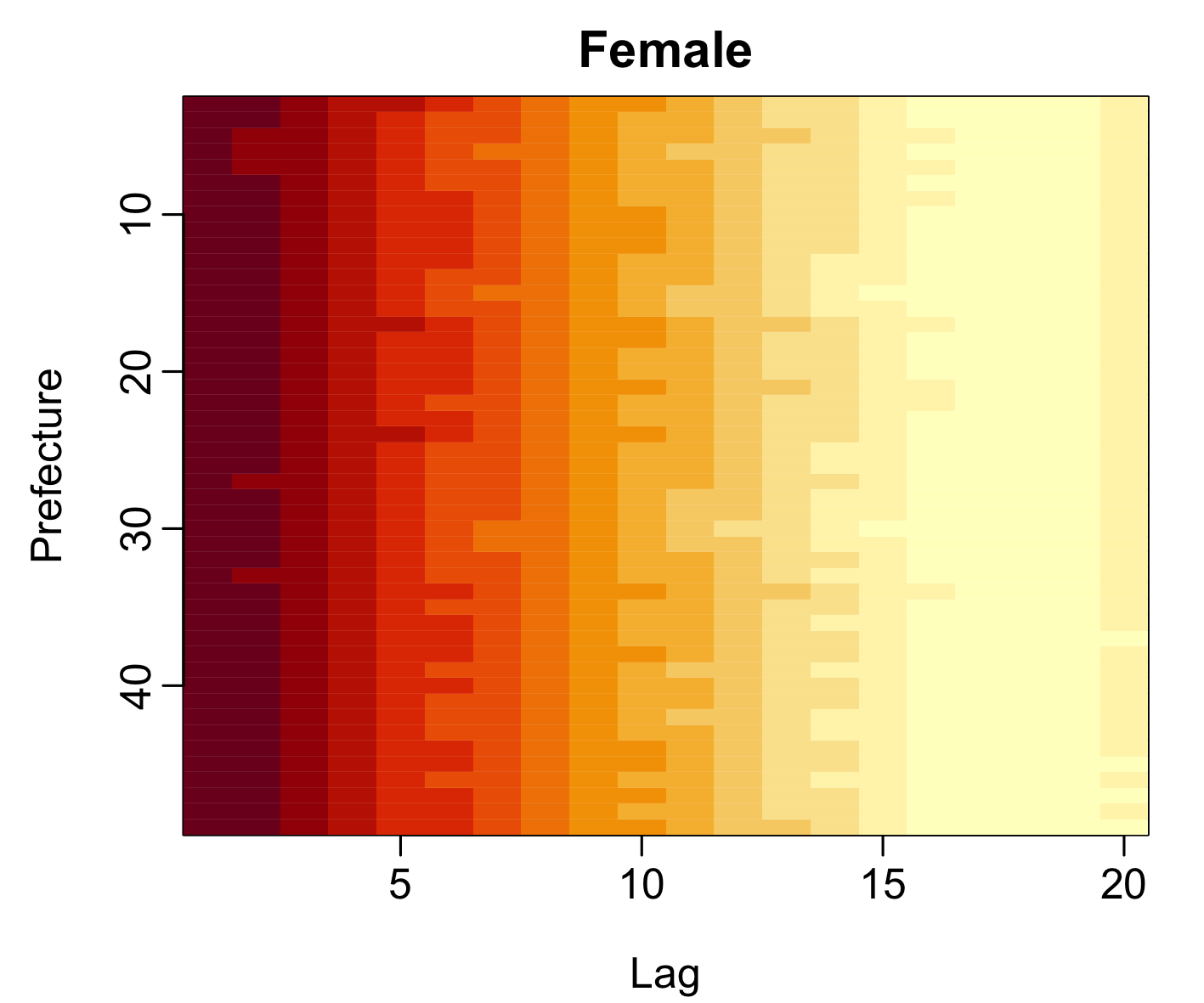
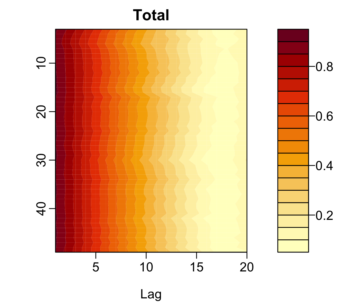
Figure 3: Functional cross-correlation plots showing the dependence of the female, male, and total life-table death counts between each prefecture and the whole country. Prefectures are numbered geographically from north to south.

3 Cumulative distribution function transformation

In the CDF transformation, we first convert an age distribution of death for each year to a probability by dividing its radix $10^{5}$. Via the cumulative sum, we transform a probability density function into a CDF,

$$D_{t,s}^{g}(u_{x})=\sum^{x}_{i=1}d_{t,s}^{g}(u_{i}),\quad x=1,\dots,111,\quad t=1,\dots,n,$$

where $D_{t,s}^{g}(u_{111})=1$. In doing so, it enjoys an additional benefit of monotonicity (see also Mayhew & Smith, 2013).

Then, we perform a logistic transformation,

$$\mathcal{X}_{t,s}^{g}(u_{x})=\text{logit}[D_{t,s}^{g}(u_{x})]=\ln\Big{[}\frac{D_{t,s}^{g}(u_{x})}{1-D_{t,s}^{g}(u_{x})}\Big{]},$$

where $\ln(\cdot)$ denotes the natural logarithm. Since $D_{t,s}^{g}(u_{111})=1$, the last column is removed to avoid the undefinedness of the logistic transformation. By considering age as a continuum, the object $\mathcal{X}_{t,s}^{g}(u)$ is an example of a high-dimensional functional time series.

To transform $\mathcal{X}_{t,s}^{g}(u_{x})$ back to the original scale, we first perform an inverse logit transformation, obtaining

$$D_{t,s}^{g}(u_{x})=\frac{\exp^{\mathcal{X}_{t,s}^{g}(u_{x})}}{1+\exp^{\mathcal{X}_{t,s}^{g}(u_{x})}},$$

where we add back the last column of ones. Then, we take the first-order differencing to obtain

$$d_{t,s}^{g}(u_{x})=\Delta_{i=1}^{x}D_{t,s}^{g}(u_{i})\times 10^{5},$$

where $\Delta$ represents the first-order differencing, where $\Delta_{i=1}^{1}D_{t,s}^{g}(u_{1})=D_{t,s}^{g}(u_{1})$. The constant $10^{5}$ is the radix of the life-table death count. Since the data are observed discretely, we use the cumulative sum and first-order differencing as approximations for integration and differentiation, respectively.

4 Functional time-series forecasting models

We obtain a set of unconstrained functional time series $(\mathcal{X}_{1,s}^{g}(u),\dots,\mathcal{X}_{n,s}^{g}(u)]$ via the CDF transformation. Generally, we represent it as $\{\mathcal{X}_{t,s}^{g}(u)\}$, which is an arbitrary functional time series defined on a common probability space. It is assumed that the observations $\mathcal{X}_{t,s}^{g}(u)$ are elements of the Hilbert space $\mathcal{H}=\mathcal{L}^{2}(\mathcal{I})$ equipped with the inner product $\langle w,v\rangle=\int_{\mathcal{I}}w(u)v(u)du$, where $u$ represents a continuum and $\mathcal{I}\subset\mathds{R}$ denotes a function support range, and $\mathds{R}$ is the real line. Each function is a square-integrable function satisfying $\|\mathcal{X}_{t,s}^{g}\|^{2}=\int_{\mathcal{I}}(\mathcal{X}_{t,s}^{g}(u))^{2}du<\infty$ and associated norms.

4.1 Univariate functional time-series (UFTS) forecasting method

We assume $\mathcal{X}_{t,s}^{g}(u)$ has a finite mean and variance. Then, its non-negative definite covariance function is given by

$$c_{s}^{g}(u,v) :=\text{Cov}[\mathcal{X}_{s}^{g}(u),\mathcal{X}_{s}^{g}(v)]$$

$$=\text{E}\left\{[\mathcal{X}_{s}^{g}(u)-\mu_{s}^{g}(u)][\mathcal{X}_{s}^{g}(v)-\mu_{s}^{g}(v)]\right\},\qquad\forall u,v\in\mathcal{I},$$

where $\mu_{s}^{g}(u)=\text{E}\{\mathcal{X}_{t,s}^{g}(u)\}$. Via Mercer’s lemma, there exists a set of orthonormal sequence $(\phi_{k})$ of continuous functions in $\mathcal{L}^{2}(\mathcal{I})$ and a non-increasing sequence $\lambda_{k,s}^{g}$ of positive numbers, such that

$$c_{s}^{g}(u,v)=\sum^{\infty}_{k=1}\lambda_{k,s}^{g}\phi_{k,s}^{g}(u)\phi_{k,s}^{g}(v),$$

where $\lambda_{k,s}^{g}$ and $\phi_{k,s}^{g}(u)$ denote the $k$^th eigenvalue and eigenfunction, respectively. The Karhunen-Loève expansion of a stochastic process $\mathcal{X}_{t,s}^{g}(u)$ can be expressed as

$$\mathcal{X}_{t,s}^{g}(u) =\mu_{s}^{g}(u)+\sum_{k=1}^{\infty}\beta_{t,k,s}^{g}\phi_{k,s}^{g}(u)$$

$$=\mu_{s}^{g}(u)+\sum_{k=1}^{K}\beta_{t,k,s}^{g}\phi_{k,s}^{g}(u)+e_{t,s}^{g}(u),$$

where the principal component score $\beta_{t,k,s}^{g}$ is given by the projection of $[\mathcal{X}_{t,s}^{g}(u)-\mu_{s}^{g}(u)]$ in the direction of the $k$^th eigenfunction $\phi_{k,s}^{g}(u)$, i.e., $\beta_{t,k,s}^{g}=\langle\mathcal{X}_{t,s}^{g}(u)-\mu_{s}^{g}(u),\phi_{k,s}^{g}(u)\rangle$; and $e_{t,s}^{g}(u)$ denotes the model error function with a mean of zero and a finite variance, and $K<n$ is the number of retained components.

There are a number of ways to select the retained number of principal components, such as the bootstrap approach proposed by Hall & Vial (2006) and Bathia et al. (2010), description length approach proposed by Poskitt & Sengarapillai (2013), pseudo-Akaike information criterion (Shibata, 1981), scree plot (Cattell, 1966), and eigenvector variability plot (Tu et al., 2009). We consider the eigenvalue ratio criterion (EVR) of Li et al. (2020), defined as

$$K=\operatorname*{arg\,min}_{k=1,\dots,k_{\max}}\left\{\frac{\widehat{\lambda}_{k+1,s}^{g}}{\widehat{\lambda}_{k,s}^{g}}\times\mathds{1}\Big{\{}\frac{\widehat{\lambda}_{k,s}^{g}}{\widehat{\lambda}_{1,s}^{g}}\geq\eta\Big{\}}+\mathds{1}\Big{\{}\frac{\widehat{\lambda}_{k,s}^{g}}{\widehat{\lambda}_{1,s}^{g}}<\eta\Big{\}}\right\},$$ (3)

where $\mathds{1}\{\cdot\}$ denotes the binary indicator function, $\eta=\frac{1}{\ln[\max(\widehat{\lambda}_{1,s}^{g},n)]}$ is a small positive value. Instead of searching through $n$, we restrict our searching range by setting $k_{\max}=\#\{k|\widehat{\lambda}_{k,s}^{g}\geq\frac{1}{n}\sum^{n}_{k=1}\widehat{\lambda}_{k,s}^{g},k\geq 1\}$. For comparison, we also consider $K=6$ as suggested in Hyndman et al. (2013).

Conditioning on the observed functions $\bm{\mathcal{X}}_{s}^{g}(u)=[\mathcal{X}_{1,s}^{g}(u),\dots,\mathcal{X}_{n,s}^{g}(u)]$ and the estimated functional principal components $\bm{B}=\big{\{}\phi_{1,s}^{g}(u),\dots,\phi_{K,s}^{g}(u)\big{\}}$, the $h$-step-ahead point forecast of $\mathcal{X}_{n+h,s}^{g}(u)$ can be expressed as

$$\widehat{\mathcal{X}}_{n+h|n,s}^{g}(u) =\text{E}\big{[}\mathcal{X}_{n+h,s}^{g}(u)|\bm{\mathcal{X}}_{s}^{g}(u),\bm{B}\big{]}$$

$$=\widehat{\mu}_{s}^{g}(u)+\sum^{K}_{k=1}\widehat{\beta}_{n+h|n,k,s}^{g}\widehat{\phi}_{k,s}^{g}(u),$$

where $\widehat{\mu}_{s}^{g}(u)=\frac{1}{n}\sum^{n}_{t=1}\mathcal{X}_{t,s}^{g}(u)$ and $\widehat{\beta}_{n+h|n,k,s}^{g}$ denotes time-series forecasts of the $k$^th principal component scores. The forecasts of these scores can be obtained via a univariate time-series forecasting method, such as exponential smoothing (Hyndman et al., 2008). Computationally, we implement the ets function in the forecast package (Hyndman & Khandakar, 2008), which selects the optimal parameters based on the corrected Akaike information criterion.

4.2 Multivariate functional time-series (MFTS) forecasting method

The univariate functional time-series method does not incorporate a correlation between female and male data within the same region. However, explicitly modeling the correlation between multiple series may improve forecast accuracy. We consider a multivariate functional time-series method to jointly model and forecast multiple series that could be correlated with each other.

Let $\mathcal{X}_{t,s}^{F}(u)$ and $\mathcal{X}_{t,s}^{M}(u)$ represent female and male subnational age distribution of death counts. As our multiple functional time series have the same function support, we consider data where each observation consists of $\omega\geq 2$ functions, that is, $[\mathcal{X}_{t,s}^{F}(u),\mathcal{X}_{t,s}^{M}(u)]\in\mathds{R}^{2}$, where $u\in\mathcal{I}$.

The multivariate functional time series are stacked in a vector. Let $\nu^{F}_{s}(u)$ and $\nu^{M}_{s}(u)$ represent the mean function. For $u,v\in\mathcal{I}$, the theoretical cross-covariance function can be defined with elements

$$c_{s}(u,v):=\text{Cov}[\mathcal{X}^{F}_{s}(u),\mathcal{X}^{M}_{s}(v)]=\text{E}\left\{[\mathcal{X}^{F}_{s}(u)-\nu^{F}_{s}(u)][\mathcal{X}^{M}_{s}(u)-\nu^{M}_{s}(u)]\right\}.$$

The Karhunen-Loève expansion of a stochastic process can be expressed as

$$\bm{\mathcal{X}}_{s}(u)=\bm{\nu}_{s}(u)+\bm{\Phi}_{s}(u)\bm{\beta}_{t,s}^{\top},$$

where $\bm{\mathcal{X}}_{s}(u)=[\bm{\mathcal{X}}_{s}^{F}(u),\bm{\mathcal{X}}_{s}^{M}(u)]$, $\bm{\mathcal{X}}_{s}^{F}(u)=[\mathcal{X}_{1,s}^{F}(u),\dots,\mathcal{X}_{n,s}^{F}(u)]$ denote stacked historical functions, and $\bm{\nu}_{s}(u)=[\bm{\nu}_{s}^{F}(u),\bm{\nu}_{s}^{M}(u)]$. Moreover, $\bm{\beta}_{s}=(\bm{\beta}_{1,s},\dots,\bm{\beta}_{K,s})$ and $\bm{\beta}_{1,s}=(\beta_{1,1,s},\dots,\beta_{n,1,s})$ is the vector of principal component scores, and

$$\bm{\Phi}_{s}(u)=\left[\begin{array}[]{cccccc}\phi_{1,s}^{F}(u)&\cdots&\phi_{K,s}^{F}(u)&&\cdots&\\ &\cdots&&\phi_{1,s}^{M}(u)&\cdots&\phi_{K,s}^{M}(u)\end{array}\right]_{2\times(K\times 2)}$$

where $K$ denotes the retained number of principal components shared by females and males.

Conditioning on the past functions $\bm{\mathcal{X}}_{s}(u)$ and the estimated functional principal components $\bm{\Phi}_{s}(u)$, the $h$-step-ahead point forecast of $\bm{\mathcal{X}}_{n+h,s}(u)$ can be expressed as

$$\widehat{\bm{\mathcal{X}}}_{n+h|n,s}(u)=\text{E}\left[\bm{\mathcal{X}}_{n+h,s}(u)|\bm{\mathcal{X}}_{s}(u),\bm{\Phi}_{s}(u)\right]=\widehat{\nu}_{s}(u)+\widehat{\bm{\Phi}}_{s}(u)\widehat{\bm{\beta}}_{n+h|n,s}^{\top},$$

where $\widehat{\bm{\beta}}_{n+h|n,s}$ denotes the time-series forecasts of the principal component scores corresponding to the female and male series, $\widehat{\nu}_{s}(u)$ and $\widehat{\bm{\Phi}}_{s}(u)$ denote the estimated mean function and estimated functional principal components, respectively.

4.3 Multilevel functional time-series (MLFTS) forecasting method

The multilevel functional data model strongly resembles to the two-way functional analysis of variance studied by Morris & Carroll (2006) and Cuesta-Albertos & Febrero-Bande (2010). The basic idea is to extract common patterns shared by multiple series $R_{t,s}(u)$ and series-specific patterns $U_{t,s}^{g}(u)$. The common trend and series-specific trend are modeled by projecting them onto the eigenvectors of covariance functions of the aggregated and series-specific stochastic processes, relatively. For $t=1,\dots,n$, a curve can be expressed as

$$\mathcal{X}_{t,s}^{g}(u)=\mu^{g}_{s}(u)+R^{c}_{t,s}(u)+U_{t,s}^{g}(u),$$ (4)

where $R^{c}_{t,s}(u)$ can be the simple average of the female and male series. To ensure model and parameter identifiability, we implement a two-stage estimation procedure based on functional principal component decomposition.

Since the stochastic processes $R^{c}_{t,s}(u)$ and $U^{g}_{t,s}(u)$ are unknown in practice, the population eigenvalues and eigenfunctions can only be approximated at best through a set of realizations $\bm{R}^{c}_{s}(u)$ and $\bm{U}_{s}^{g}(u)$. From the covariance function of $\bm{R}^{c}_{s}(u)$, we can extract a set of functional principal components and their associated scores, along with a set of residual functions. From the covariance function of the residuals, we can then extract a second set of functional principal components and their associated scores. While the first functional principal component decomposition captures the common pattern across multiple series, the second functional principal component decomposition captures the series-specific residual trend.

The sample versions of series-specific mean function, a common trend and series-specific residual trend for a set of functional time series can be estimated by

$$\widehat{\mu}_{s}^{g}(u) =\frac{1}{n}\sum^{n}_{t=1}\mathcal{X}_{t,s}^{g}(u)$$ (5)

$$R_{t,s}^{c}(u) \approx\sum^{K}_{k=1}\beta_{t,k,s}^{c}\phi_{k,s}^{c}(u)$$ (6)

$$U_{t,s}^{g}(u) \approx\sum^{L}_{l=1}\gamma_{t,l,s}^{g}\psi_{l,s}^{g}(u),$$ (7)

where $\widehat{\mu}^{g}_{s}(u)$ represents the simple average of the female or male series, $\bm{\beta}_{k,s}^{c}=(\beta_{1,k,s}^{c},\dots,\beta_{n,k,s}^{c})$ represents the $k$^th sample principal component scores of $\bm{R}^{c}_{s}(u)$, and $\bm{\gamma}_{l,s}^{g}=(\gamma_{1,l,s}^{g},\dots,\gamma_{n,l,s}^{g})$ represents the $l$^th sample principal component scores of $\bm{U}_{s}^{g}(u)$.

Plugging (5) to (7) into (4), we obtain

$$\mathcal{X}_{t,s}^{g}(u)\approx\widehat{\mu}^{g}_{s}(u)+\sum^{K}_{k=1}\beta_{t,k,s}^{c}\phi_{k,s}^{c}(u)+\sum^{L}_{l=1}\gamma_{t,l,s}^{g}\psi_{l,s}^{g}(u)+e_{t,s}^{g}(u),$$

where $e_{t,s}^{g}(u)$ denotes measurement error with a finite variance.

To select the retained number of components, we use the eigenvalue ratio criterion in (3). A feature of the multilevel method is its ability to estimate the proportion of variability explained by aggregated data. For a given population $g$, a measure of the within-cluster variability is given by

$$\frac{\sum_{k=1}^{K}\widehat{\lambda}_{k,s}^{c}}{\sum_{k=1}^{K}\widehat{\lambda}_{k,s}^{c}+\sum_{l=1}^{L}\widehat{\lambda}_{l,s}^{g}}.$$

When the common trend can explain the primary mode of total variability, the value of the within-cluster variability is close to 1.

Conditioning on observed data $\bm{\mathcal{X}}^{g}_{s}(u)$ and basis functions $\bm{\Phi}_{s}(u)$ and $\bm{\Psi}_{s}^{g}(u)=\{\widehat{\psi}_{1,s}^{g}(u)$,$\dots$,$\widehat{\psi}_{L,s}^{g}(u)\}$, the $h$-step-ahead forecasts can be obtained by

$$\widehat{\mathcal{X}}_{n+h|n,s}^{g}(u) =\text{E}[\mathcal{X}_{n+h,s}^{g}(u)|\mu^{g}_{s}(u),\bm{\mathcal{X}}^{g}_{s}(u),\bm{\Phi}_{s}(u),\bm{\Psi}_{s}^{g}(u)]$$

$$=\widehat{\mu}^{g}_{s}(u)+\sum^{K}_{k=1}\widehat{\beta}_{n+h|n,k,s}^{c}\widehat{\phi}_{k,s}^{c}(u)+\sum^{L}_{l=1}\widehat{\gamma}_{n+h|n,l,s}^{g}\widehat{\psi}_{l,s}^{g}(u),$$

where $\widehat{\mu}_{s}^{g}(u)=\frac{1}{n}\sum^{n}_{t=1}\mathcal{X}_{t,s}^{g}(u)$, $\{\widehat{\beta}_{n+h|n,k,s}^{c},k=1,\dots,K\}$ and $\{\widehat{\gamma}_{n+h|n,l,s}^{g},l=1,\dots,L\}$ are the forecasted principal component scores, obtained from a univariate time-series forecasting method.

4.4 Two-way functional analysis of variance

To model $\mathcal{X}_{t,s}^{g}(u)$, we consider a two-way functional ANOVA decomposition, expressed as:

$$\mathcal{X}_{t,s}^{g}(u)=\mu(u)+\alpha_{s}(u)+\beta^{g}(u)+\epsilon_{t,s}^{g}(u),$$

where $\mu(u)$ denotes the functional grand effect, $\alpha_{s}(u)$ denotes the functional row effect, $\beta^{g}(u)$ denotes the functional column effect, and $\epsilon_{t,s}^{g}(u)$ denotes the error function.

The functional ANOVA model can be estimated by means with

$$\widehat{\mu}(u) =\frac{1}{n_{s}\times 2\times n}\sum^{n_{s}}_{s=1}\sum^{2}_{g=1}\sum^{n}_{t=1}\mathcal{X}_{t,s}^{g}(u)$$

$$\widehat{\alpha}_{s}(u) =\frac{1}{2\times n}\sum^{2}_{g=1}\sum^{n}_{t=1}\mathcal{X}_{t,s}^{g}(u)-\widehat{\mu}(u)$$

$$\widehat{\beta}^{g}(u) =\frac{1}{n_{s}\times n}\sum^{n_{s}}_{s=1}\sum^{n}_{t=1}\mathcal{X}_{t,s}^{g}(u)-\widehat{\mu}(u).$$

Some identifiability constraints exist, $\forall u\in\mathcal{I}$, $\sum^{n_{s}}_{s=1}\alpha_{s}(u)=\sum^{2}_{g=1}\beta^{g}(u)=0$, and $\sum^{n_{s}}_{s=1}\mathcal{X}_{t,s}^{g}(u)=\sum^{2}_{g=1}\mathcal{X}_{t,s}^{g}(u)=0$, $\forall t$.

The residual functions $\widehat{\epsilon}_{t,s}^{g}(u)=\mathcal{X}_{t,s}^{g}(u)-\widehat{\mu}(u)-\widehat{\alpha}_{s}(u)-\widehat{\beta}^{g}(u)$ are time-varying, for $t=1,\dots,n$. Following Jiménez-Varón et al. (2024), we model and forecast the residual functions via the MFTS.

4.5 Two-stage functional principal component analyses

Gao et al. (2019) propose a two-stage functional principal component decomposition to model and forecast HDFTS. One of the earliest methods for comparison (see, e.g., Tavakoli et al., 2023; Shang, 2025), it consists of three parts.

1. Functional principal component analysis is performed separately on each set of functional time series, resulting in $P$ sets of principal component scores of low dimension $p_{0}$.

2. The first functional principal component scores from each of $P$ sets of functional time series are combined into an $P\times 1$ vector. We fit factor models to the scores to further reduce the dimension into an $r\times 1$ vector, where $r<<P$. The same is carried out for the second, third, and so on until the $p_{0}$^th scores. The vector of $P$ functional time series is reduced to an $r\times p_{0}$ matrix consisting of factors.

3. A univariate time series model can be fitted to each factor and forecasts are generated. The forecast factors can be used to construct forecast functions.

5 Construction of prediction intervals

We equally split the data sample consisting of 48 years from 1975 to 2022 into training, validation, and testing sets, each consisting of 16 years. Using the data in the training sample, we implement an expanding window forecast scheme to obtain the $h$-step-ahead density forecasts in the validation set for $h=1,2,\dots,15$. For each horizon, we have different numbers of curves in the validation set. For instance, when $h=1$, we have 16 years to evaluate the forecast errors, denoted by $\widehat{\epsilon}_{m,s}^{g}(u)=d_{m,s}^{g}(u)-\widehat{d}_{m,s}^{g}(u)$ for $m=1,2,\dots,M=16$; when $h=15$, we have two years to evaluate the residual functions between the samples in the validation set and their corresponding forecasts. From these residual functions, we compute the functional standard deviation, denoted by

$$\gamma(u)=\text{sd}[\widehat{\epsilon}_{1,s}^{g}(u),\dots,\widehat{\epsilon}_{M,s}^{g}(u)].$$ (8)

We aim to determine $(\overline{\xi}_{\alpha},\underline{\xi}_{\alpha})$ such that $\alpha\times 100\%$ of the residuals satisfy

$$-\underline{\xi}_{\alpha}\gamma(u)\leq\widehat{\epsilon}_{m,s}^{g}(u)\leq\overline{\xi}_{\alpha}\gamma(u),$$

where $(\overline{\xi}_{\alpha},\underline{\xi}_{\alpha})$ are the tuning parameters.

Typically, the constants $\overline{\xi}_{\alpha}$ and $\underline{\xi}_{\alpha}$ are chosen equal. By a law of large numbers, one may achieve

$$\text{Pr}\left[-\xi_{\alpha}\gamma(u)\leq d_{n+h,s}^{g}(u)-\widehat{d}_{n+h,s}^{g}(u)\leq\xi_{\alpha}\gamma(u)\right]\approx\frac{1}{M}\sum^{M}_{m=1}\mathds{1}\left[-\xi_{\alpha}\gamma(u)\leq\widehat{\epsilon}_{m,s}^{g}(u)\leq\xi_{\alpha}\gamma(u)\right],$$

where $\mathds{1}(\cdot)$ denotes binary indicator function and $M$ denotes the number of years in the validation set.

To determine the optimal $\xi_{\alpha}$, the samples in the validation set are used to calibrate the prediction intervals so that the empirical coverage probabilities defined in (10) are close to their nominal coverage probabilities.

In Appendix C, we also present the conformal prediction interval approach of Shafer & Vovk (2008) that does not require the tuning parameter. Essentially, by considering a quantile of the absolute residual functions, the pointwise prediction interval for the out-of-sample testing set is centered around the point forecast, with its spread determined by the chosen quantile.

6 Results

6.1 Expanding window scheme

An expanding window analysis of a time-series model is commonly used to assess model and parameter stability and prediction accuracy over time. The expanding window analysis determines the constancy of a model’s parameter by computing parameter estimates and their forecasts over an expanding window through the sample (for details, see Zivot & Wang, 2006, pp. 313–314).

Using the first 32 years from 1975 to 2006 in the Japanese subnational age- and sex-specific life-table death counts, we produce one- to 16-step-ahead forecasts. Through an expanding-window approach, we re-estimate the parameters in the time-series forecasting models using the first 33 years from 1975 to 2007. Forecasts from the estimated models are then produced for one- to 15-step-ahead forecasts. We iterate this process by increasing the sample size by one year until reaching the end of the data period in 2022. This process produces 16 one-step-ahead forecasts, 15 two-step-ahead forecasts, $\dots$, and one 16-step-ahead forecast. We compare these forecasts with the holdout samples to determine the out-of-sample forecast accuracy. In Figure 4, we display a diagram of the expanding window forecast scheme for forecast horizon $h=1$, although we also consider other forecast horizons from $h=2$ to $16$.

[-¿] (0,0) – (10,0) node[right] Time;

[fill=blue!20] (0,-0.5) rectangle (3,0.5) node[midway] Train; [fill=red!20] (3,-0.5) rectangle (3.5,0.5) node[midway] F;

[fill=blue!20] (0,-1.5) rectangle (5,-0.5) node[midway] Train; [fill=red!20] (5,-1.5) rectangle (5.5,-0.5) node[midway] F;

[fill=blue!20] (0,-2.5) rectangle (7,-1.5) node[midway] Train; [fill=red!20] (7,-2.5) rectangle (7.5,-1.5) node[midway] F;

[fill=blue!20] (0,-3.5) rectangle (9,-2.5) node[midway] Train; [fill=red!20] (9,-3.5) rectangle (9.5,-2.5) node[midway] F;

[left] at (0,0) 1975:2006; [left] at (0,-1) 1975:2007; [left] at (0,-2) $\vdots$; [left] at (0,-3) 1975:2021;

[fill=blue!20] (6.5,1) rectangle (7,1.5); [right] at (7,1.25) Training Window; [fill=red!20] (6.5,0.5) rectangle (7,1); [right] at (7,0.75) Forecast (F);

Figure 4: A diagram of the expanding-window forecast scheme.

6.2 Point forecast error metrics

Since life-table death counts can be considered a probability density function, we utilize some density evaluation measures. These measures include the discrete version of the KLD (Kullback & Leibler, 1951), the square root of the JSD (Shannon, 1948). For two probability density functions, denoted by $d_{m+\xi}$ and $\widehat{d}_{m+\xi}$, the symmetric version of the KLD, also known as Jeffrey divergence, is defined as

$$\text{KLD}(h)=\ \text{D}_{\text{KL}}(d_{m+\xi}||\widehat{d}_{m+\xi})+\text{D}_{\text{KL}}(\widehat{d}_{m+\xi}||d_{m+\xi})$$

$$=\ \frac{1}{111\times(17-h)}\sum^{16}_{\xi=h}\sum_{x=1}^{111}d_{m+\xi}(u_{x})\cdot\left[\ln d_{m+\xi}(u_{x})-\ln\widehat{d}_{m+\xi}(u_{x})\right]+$$

$$\frac{1}{111\times(17-h)}\sum^{16}_{\xi=h}\sum_{x=1}^{111}\widehat{d}_{m+\xi}(u_{x})\cdot\left[\ln\widehat{d}_{m+\xi}(u_{x})-\ln d_{m+\xi}(u_{x})\right],$$ (9)

which is non-negative, for $h=1,2,\dots,16$.

An alternative metric is the JSD, defined by

$$\text{JSD}(h)=\frac{1}{2}D_{\text{KL}}(d_{m+\xi}||\delta_{m+\xi})+\frac{1}{2}D_{\text{KL}}(\widehat{d}_{m+\xi}||\delta_{m+\xi}),$$

where $\delta_{m+\xi}$ measures a common quantity between $d_{m+\xi}$ and $\widehat{d}_{m+\xi}$. Following the early work of Shang & Haberman (2020), we consider the geometric mean $\delta_{m+\xi}=\sqrt{d_{m+\xi}\widehat{d}_{m+\xi}}$. To make the JSD a metric between two probability densities, we take the square root of the JSD (see, e.g., Fuglede & Topsoe, 2004).

6.3 Comparison of point forecast accuracy

In Table LABEL:tab:1, averaged across 47 prefectures, we compare the point forecast accuracy among the functional time-series models. From the summary statistics of the KLD and JSD, the HDFPCA model offers the most accurate point forecasts for the female data. For the male data, the MFTS and MLFTS models provide the most accurate point forecasts. For the UFTS, MFTS, MLFTS, and FANOVA models, the number of retained functional principal components was determined by the EVR criterion. For the HDFPCA model, we follow the default setting of Gao et al. (2019), where the number of retained components is six and two in the first and second stages, respectively. In Appendix A, we also provide the results for $K=6$.

Table 1: Averaged across 47 prefectures, we evaluate and compare the point forecast accuracy, measured by the KLD and JSD, among the functional time-series models. The number of components is determined by the EVR criterion.

		Female					Male
Metric	$h$	UFTS	MFTS	MLFTS	FANOVA	HDFPCA	UFTS	MFTS	MLFTS	FANOVA	HDFPCA
KLD	1	0.006	0.010	0.006	0.006	0.008	0.005	0.005	0.004	0.005	0.004
	2	0.007	0.011	0.006	0.007	0.010	0.006	0.006	0.005	0.005	0.005
	3	0.009	0.013	0.007	0.008	0.010	0.007	0.007	0.005	0.006	0.006
	4	0.011	0.014	0.009	0.010	0.011	0.007	0.007	0.006	0.007	0.006
	5	0.013	0.016	0.010	0.012	0.012	0.008	0.008	0.007	0.008	0.007
	6	0.016	0.017	0.011	0.013	0.010	0.009	0.009	0.008	0.008	0.008
	7	0.019	0.019	0.013	0.016	0.015	0.011	0.010	0.008	0.009	0.009
	8	0.024	0.021	0.016	0.019	0.012	0.012	0.011	0.010	0.010	0.010
	9	0.030	0.024	0.019	0.024	0.018	0.013	0.013	0.011	0.011	0.011
	10	0.037	0.028	0.023	0.029	0.011	0.014	0.014	0.012	0.012	0.012
	11	0.042	0.033	0.025	0.034	0.024	0.015	0.016	0.011	0.012	0.014
	12	0.049	0.027	0.029	0.037	0.009	0.016	0.011	0.011	0.011	0.016
	13	0.058	0.032	0.037	0.046	0.031	0.017	0.012	0.014	0.013	0.019
	14	0.072	0.039	0.045	0.055	0.011	0.018	0.014	0.016	0.015	0.023
	15	0.098	0.047	0.061	0.076	0.045	0.019	0.015	0.021	0.021	0.032
	16	0.130	0.059	0.091	0.104	0.015	0.020	0.017	0.031	0.028	0.044
	Mean	0.039	0.026	0.026	0.031	0.016	0.012	0.011	0.011	0.011	0.014
	Median	0.027	0.023	0.017	0.021	0.011	0.012	0.011	0.010	0.011	0.010
JSD	1	0.038	0.048	0.037	0.044	0.038	0.035	0.034	0.031	0.033	0.034
	2	0.042	0.051	0.040	0.046	0.041	0.038	0.036	0.034	0.035	0.036
	3	0.045	0.054	0.043	0.049	0.044	0.040	0.039	0.036	0.037	0.038
	4	0.051	0.057	0.046	0.048	0.048	0.043	0.041	0.038	0.040	0.040
	5	0.056	0.060	0.050	0.056	0.052	0.046	0.043	0.041	0.042	0.042
	6	0.061	0.061	0.053	0.050	0.056	0.049	0.045	0.043	0.044	0.043
	7	0.066	0.063	0.057	0.062	0.060	0.052	0.047	0.045	0.047	0.045
	8	0.073	0.066	0.061	0.053	0.065	0.055	0.049	0.047	0.049	0.047
	9	0.081	0.070	0.067	0.070	0.071	0.057	0.052	0.049	0.052	0.049
	10	0.089	0.074	0.073	0.054	0.078	0.060	0.054	0.052	0.056	0.051
	11	0.099	0.079	0.078	0.080	0.086	0.062	0.056	0.053	0.061	0.052
	12	0.109	0.080	0.085	0.053	0.095	0.063	0.054	0.055	0.066	0.053
	13	0.121	0.086	0.095	0.093	0.105	0.065	0.057	0.059	0.073	0.057
	14	0.134	0.092	0.104	0.056	0.114	0.068	0.060	0.063	0.079	0.060
	15	0.159	0.100	0.123	0.112	0.136	0.071	0.062	0.072	0.094	0.070
	16	0.188	0.115	0.151	0.066	0.162	0.073	0.065	0.086	0.113	0.083
	Mean	0.088	0.072	0.073	0.062	0.078	0.055	0.050	0.050	0.058	0.050
	Median	0.077	0.068	0.064	0.055	0.068	0.056	0.050	0.048	0.051	0.050

Figure 5 presents two heatmaps comparing seven functional time-series models across 16 forecast horizons for both female and male data. For each horizon, we count how often each method produces the smallest point forecast errors, as measured by the KLD. Choosing $K=6$ has a slight advantage compared to the one based on the EVR criterion. For shorter forecast horizons, the UFTS, MFTS, and MLFTS models perform equally well for the female data. However, for relatively longer forecast horizons, the HDFPCA model is recommended. In the case of male data, the MLFTS model is generally preferred; only at the shorter forecast horizon is $K=6$ advantageous. For relatively longer forecast horizons, the FANOVA with the EVR criterion is recommended.

(a) Female data

(b) Male data

Figure 5: Heatmaps comparing the point forecast accuracy, measured by the KLD, between nine functional time-series models across 16 forecast horizons for the testing female and male data. Since there are 47 prefectures, each row sums to 47. A method appearing more than five times is highlighted in green, while those appearing fewer than five times are shown in red. If a method appears exactly five times, it is displayed in white.

6.4 Interval forecast error metrics

To evaluate interval forecast accuracy, we consider the CPD between the empirical coverage probability (ECP) and nominal coverage probability, as well as the mean interval score of Gneiting & Raftery (2007). For each year in the forecasting period, the $h$-step-ahead prediction intervals are computed at the $100(1-\alpha)\%$ nominal coverage probability. We consider the common case of the symmetric $100(1-\alpha)\%$ prediction intervals, with lower and upper bounds that are quantiles at $\alpha/2$ and $1-\alpha/2$, denoted by $\widehat{d}_{n+\xi,s}^{g,\text{lb}}(u)$ and $\widehat{d}_{n+\xi,s}^{g,\text{ub}}(u)$. The ECP and CPD are defined as

$$\text{ECP}_{h} =\frac{1}{111\times(16-h)}\times\sum_{\xi=h}^{15}\sum_{u=1}^{111}\mathds{1}\left\{\widehat{d}_{\nu+\xi,s}^{g,\text{lb}}(u)\leq d_{\nu+\xi,s}^{g}(u)\leq\widehat{d}_{\nu+\xi,s}^{g,\text{ub}}(u)\right\},$$ (10)

$$\text{CPD}_{h} =\frac{1}{111\times(16-h)}\times\sum_{\xi=h}^{15}\sum_{u=1}^{111}\left[\mathds{1}\{d_{\nu+\xi,s}^{g}(u)>\widehat{d}_{\nu+\xi,s}^{g,\text{ub}}(u)\}+\mathds{1}\{d_{\nu+\xi,s}^{g}(u)<\widehat{d}_{\nu+\xi,s}^{g,\text{lb}}(u)\}\right],$$

where $h=1,\dots,15$, $v$ denotes the end of training set when we calibrate the CPD or interval score, and $\nu$ denotes the end of validation set when we evaluate the interval forecast accuracy.

For different ages and years in the testing set, the mean and median CPD are defined as

$$\overline{\text{CPD}} =\frac{1}{15}\sum^{15}_{h=1}\text{CPD}_{h},$$

M[CPD] $$=\text{median}(\text{CPD}_{h}).$$

As defined by Gneiting & Raftery (2007), a scoring rule for the prediction intervals at age $u$ is

$$S_{\alpha,\xi}\left[\widehat{d}^{g,\text{lb}}_{\nu+\xi,s}(u),\widehat{d}^{g,\text{ub}}_{\nu+\xi,s}(u),d^{g}_{\nu+\xi,s}(u)\right] =\left[\widehat{d}^{g,\text{ub}}_{\nu+\xi,s}(u)-\widehat{d}^{g,\text{lb}}_{\nu+\xi,s}(u)\right]$$

$$+\frac{2}{\alpha}\left[\widehat{d}^{g,\text{lb}}_{\nu+\xi,s}(u)-d_{n+\xi,s}^{g}(u)\right]\mathds{1}\left\{d_{\nu+\xi,s}^{g}(u)<\widehat{d}_{\nu+\xi,s}^{g,\text{lb}}(u)\right\}$$

$$+\frac{2}{\alpha}\left[d_{\nu+\xi,s}^{g}(u)-\widehat{d}_{\nu+\xi,s}^{g,\text{ub}}(u)\right]\mathds{1}\left\{d_{\nu+\xi,s}^{g}(u)>\widehat{d}_{\nu+\xi,s}^{g,\text{ub}}(u)\right\},$$

where the level of significance is customarily set to be $\alpha=0.2$ or 0.05. The interval score rewards a narrow prediction interval width if and only if $100(1-\alpha)\%$ of the holdout densities lie within the prediction interval.

For different ages and years in the testing set, the mean interval score is defined by

$$\overline{S}_{\alpha}(h)=\frac{1}{111\times(16-h)}\times\sum^{15}_{\xi=h}\sum^{111}_{u=1}S_{\alpha,\xi}\left[\widehat{d}_{\nu+\xi,s}^{g,\text{lb}}(u),\widehat{d}_{\nu+\xi,s}^{g,\text{ub}}(u),d_{\nu+\xi,s}^{g}(u)\right].$$

Averaging over all forecast horizons, we obtain the overall mean interval score

$$\overline{S}_{\alpha} =\frac{1}{15}\sum^{15}_{h=1}\overline{S}_{\alpha}(h),$$

$$\text{M}[S_{\alpha}] =\text{median}[\overline{S}_{\alpha}(h)].$$

6.5 Comparison of interval forecast accuracy

In Table LABEL:tab:2, averaged across 47 prefectures, we compare the interval forecast accuracy among the functional time-series models using the EVR criterion. From the summary statistics of the CPD and interval score at the level of significance $\alpha=0.2$, the MFTS offers the smallest CPD value for the female data, while the UFTS and MLFTS offer the smallest CPD values for the male data. In terms of the interval scores, the HDFPCA provides the smallest interval scores for the female data, while the MLFTS gives the smallest interval scores for the male data. In Appendix B, we also provide the results for $K=6$.

Table 2: Averaged across 47 prefectures, we evaluate and compare the interval forecast accuracy, as measured by the CPD and interval score, among the seven functional time-series models at the level of significance $\alpha=0.2$. The number of components is determined by the EVR criterion.

		Female					Male
Metric	$h$	UFTS	MFTS	MLFTS	FANOVA	HDFPCA	UFTS	MFTS	MLFTS	FANOVA	HDFPCA
$\overline{\text{CPD}}_{0.2}$	1	0.061	0.065	0.043	0.075	0.072	0.056	0.085	0.044	0.074	0.059
	2	0.067	0.058	0.045	0.088	0.053	0.058	0.088	0.047	0.079	0.071
	3	0.071	0.054	0.052	0.097	0.074	0.055	0.090	0.052	0.088	0.073
	4	0.081	0.051	0.058	0.117	0.076	0.054	0.094	0.057	0.093	0.084
	5	0.087	0.048	0.065	0.122	0.091	0.056	0.096	0.061	0.098	0.086
	6	0.086	0.045	0.069	0.128	0.100	0.058	0.095	0.058	0.095	0.090
	7	0.090	0.047	0.071	0.130	0.069	0.057	0.091	0.056	0.087	0.084
	8	0.095	0.046	0.074	0.131	0.107	0.060	0.085	0.056	0.089	0.075
	9	0.096	0.050	0.080	0.131	0.060	0.072	0.083	0.060	0.087	0.076
	10	0.104	0.052	0.088	0.143	0.138	0.073	0.082	0.063	0.087	0.086
	11	0.103	0.051	0.082	0.144	0.048	0.075	0.086	0.074	0.084	0.084
	12	0.105	0.059	0.087	0.136	0.134	0.069	0.083	0.067	0.080	0.077
	13	0.106	0.061	0.093	0.137	0.048	0.069	0.082	0.080	0.080	0.080
	14	0.116	0.067	0.094	0.145	0.096	0.065	0.079	0.076	0.089	0.077
	15	0.122	0.069	0.093	0.137	0.086	0.057	0.067	0.071	0.070	0.085
	Mean	0.093	0.055	0.073	0.118	0.083	0.062	0.086	0.062	0.085	0.079
	Median	0.095	0.052	0.074	0.131	0.076	0.058	0.085	0.060	0.087	0.080
$\overline{S}_{0.2}$	1	255	393	246	279	314	271	270	213	263	243
	2	299	417	279	328	344	298	296	237	283	270
	3	345	445	312	384	369	325	322	259	300	292
	4	412	476	353	470	361	356	351	286	321	321
	5	477	511	397	551	464	390	376	309	345	349
	6	549	543	429	639	381	419	397	331	358	370
	7	626	565	476	734	537	445	412	353	375	387
	8	721	600	536	843	420	465	433	378	393	409
	9	829	650	606	973	625	493	451	402	416	436
	10	956	725	690	1133	476	525	481	432	439	488
	11	1070	798	767	1271	793	543	506	430	455	519
	12	1199	788	864	1429	500	570	467	451	460	560
	13	1350	874	1000	1623	966	583	492	507	510	623
	14	1501	945	1108	1823	546	661	547	582	571	669
	15	1888	1122	1419	2224	1258	875	690	811	835	933
	Mean	832	657	632	1000	557	481	433	399	420	458
	Median	721	600	536	843	476	465	433	378	393	409

In Figure 6, we present two heatmaps comparing seven functional time-series models across 15 forecast horizons for both female and male testing data. For each horizon, we count how often each method produces the smallest interval forecast errors, as measured by the CPD and interval score. By examining the CPD results, we recommend the MFTS for the female data and the MLFTS model for the male data, especially for $K=6$. By examining the interval score results, we recommend the MFTS for shorter horizons and the HDFPCA for longer horizons in the female data. For the male data, the MLFTS generally provides the smallest interval scores.

(a) CPD for females

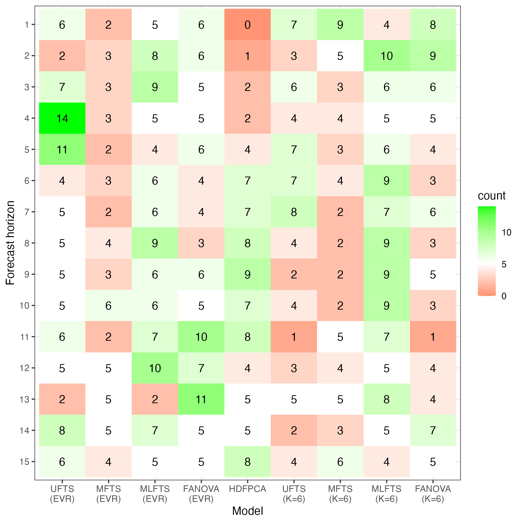
(b) CPD for males

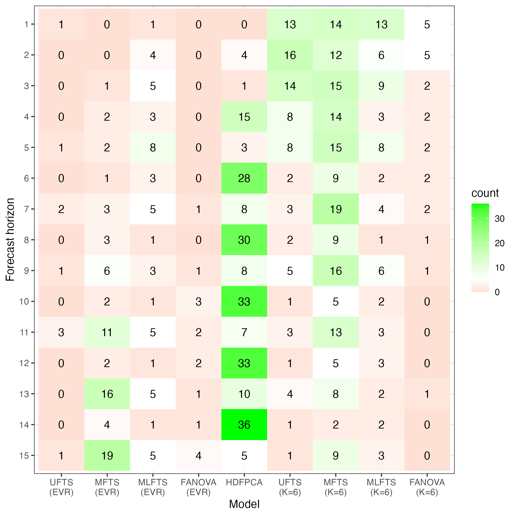
(c) Interval score for females

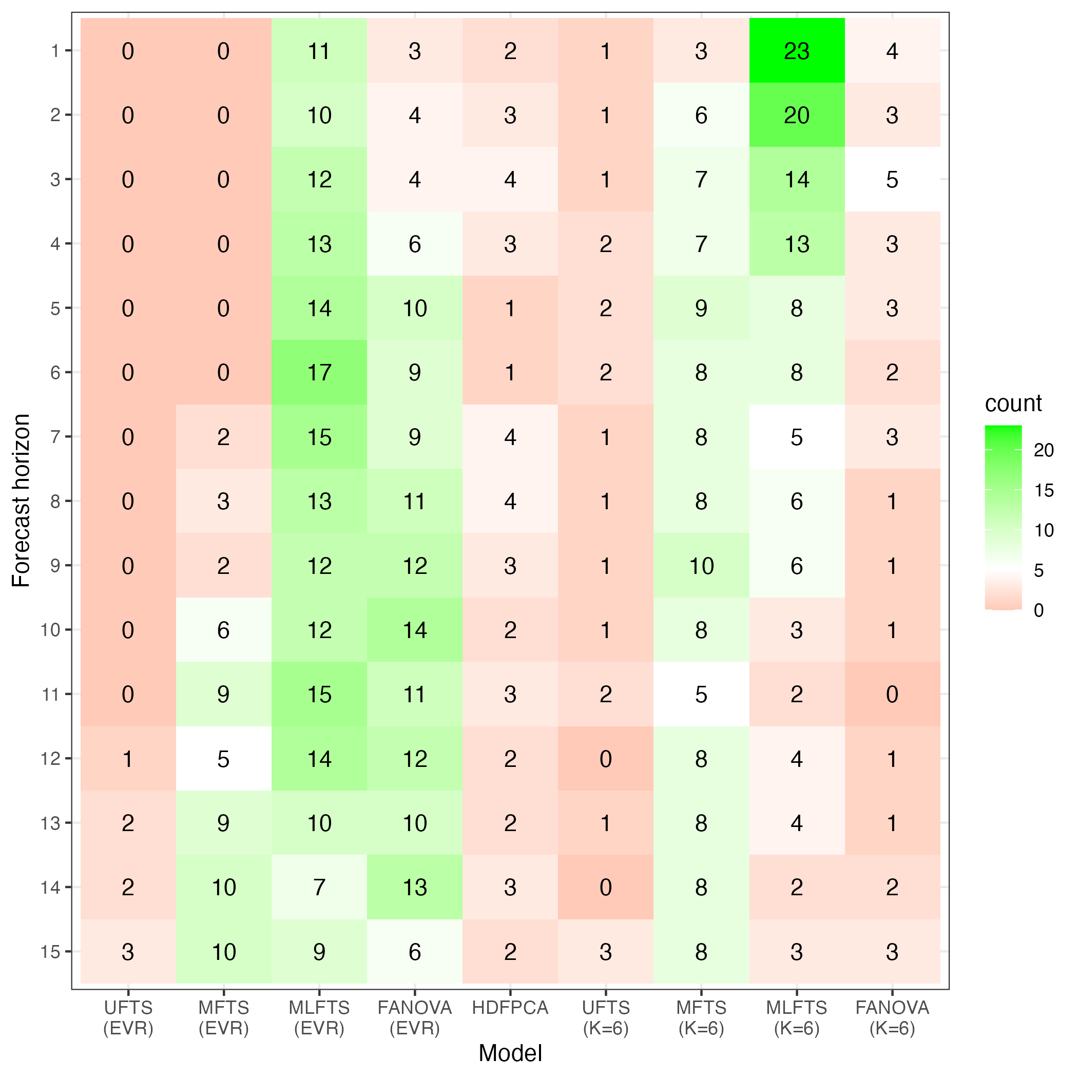
(d) Interval score for males

Figure 6: Heatmaps comparing the interval forecast accuracy at the level of significance $\alpha=0.2$, measured by the CPD and interval score, between seven functional time-series models across 15 forecast horizons for the female and male testing data. Since there are 47 prefectures, each row sums to 47. A method appearing more than five times is shown in green, while those appearing fewer than five times are shown in red. If a method appears exactly five times, it is shown in white.

The interval forecast results at the significance level of $\alpha=0.05$ are available and can be viewed in a developed Shiny app at https://cfjimenezv.shinyapps.io/Shiny_App_CDF/.

7 Conclusion

We present several graphical tools, namely image plots and cross-correlation plots, to visualize the differences and dependence in life-table death counts between each prefecture and Japan as a whole.

Via the CDF transformation, we consider a suite of functional time-series models to model and forecast subnational age distribution of death counts for 47 Japanese prefectures. The CDF transformation is ideal to handle the zero values in the subnational data. Within the CDF transformation, we also present two general strategies for constructing pointwise prediction intervals.

By dividing the datasets into training and testing samples, we evaluate and compare point and interval forecast accuracy among the functional time-series models. We confirm the importance of joint modeling techniques, in which the MFTS, MLFTS, FANOVA, and HDFPCA models generally perform well on the aggregate level across 47 prefectures. We present a novel heatmap to show the frequency (of 47 prefectures), in which one method performs the best for each forecast horizon. The individual forecast errors for various horizons, obtained from all methods for each prefecture, are available in a developed shiny app at https://cfjimenezv.shinyapps.io/Shiny_App_CDF/.

There are several ways the methodology can be further extended, and we briefly list four. First, the functional standard deviation in (8) was computed coordinate-wise. A range of functional depth exists, which can be implemented to compute other variants of standard deviations. Second, instead of symmetric prediction intervals, asymmetric ones can be considered, searching for two tuning parameters to adjust the lower and upper bounds. Third, the data set was divided equally into the training, validation, and testing samples. Other proportions may be possible and lead to a more accurate selection of tuning parameter $\xi_{\alpha}$ and more accurate interval forecasts. Fourth, to demonstrate we implemented a suite of functional time-series models. Other time-series extrapolation models may also be considered, such as the robust functional principal component analysis by Oguamalam et al. (2025). It extends Mahalanobis distance to Bayes spaces and introduces a regularized approach for improved principal component estimation in the presence of outliers.

Supplementary Materials

1. Code for the forecasting methods based on the CDF transformation.The  code to produce point and interval forecasts from the different functional time-series models described in the paper. The  codes are available at the following repository: https://github.com/cfjimenezv07/HDFTS_CDF/tree/main/Rcode

2. Code for shiny application.The  code to produce a shiny user interface for the point and interval forecasts for the 47 Japanese prefectures. The  codes are available at the following repository: https://github.com/cfjimenezv07/HDFTS_CDF/tree/main/Shiny_App_CDF

Appendix A: Point forecast accuracy when $K=6$

In Table LABEL:tab:appendix_1, averaged across 47 prefectures, we compare the point forecast accuracy among the functional time-series models, when the number of retained components is set to be six as in Hyndman et al. (2013). From the summary statistics of the KLD and JSD, the MFTS offers the most accurate point forecasts for the female and male data.

Table 3: Averaged across 47 prefectures, we evaluate and compare the point forecast accuracy, measured by the KLD and JSD, among the functional time-series models. The number of components is determined by setting $K=6$.

		Female				Male
Metric	$h$	UFTS	MFTS	MLFTS	FANOVA	UFTS	MFTS	MLFTS	FANOVA
KLD	1	0.005	0.006	0.005	0.005	0.004	0.004	0.004	0.004
	2	0.007	0.007	0.006	0.006	0.005	0.005	0.004	0.005
	3	0.008	0.008	0.007	0.008	0.006	0.005	0.005	0.005
	4	0.010	0.010	0.009	0.009	0.007	0.006	0.006	0.006
	5	0.013	0.012	0.011	0.011	0.008	0.007	0.007	0.007
	6	0.015	0.013	0.012	0.013	0.009	0.008	0.008	0.008
	7	0.018	0.015	0.014	0.016	0.010	0.009	0.009	0.009
	8	0.023	0.017	0.017	0.019	0.011	0.010	0.010	0.010
	9	0.029	0.021	0.021	0.024	0.012	0.011	0.011	0.012
	10	0.035	0.025	0.025	0.029	0.013	0.013	0.012	0.013
	11	0.041	0.029	0.028	0.034	0.014	0.014	0.011	0.013
	12	0.048	0.026	0.033	0.039	0.015	0.010	0.012	0.012
	13	0.057	0.032	0.042	0.048	0.016	0.011	0.014	0.014
	14	0.070	0.040	0.049	0.057	0.018	0.013	0.016	0.015
	15	0.096	0.050	0.068	0.079	0.019	0.014	0.020	0.021
	16	0.128	0.067	0.097	0.108	0.020	0.016	0.029	0.028
	Mean	0.038	0.024	0.028	0.032	0.012	0.010	0.011	0.011
	Median	0.026	0.019	0.019	0.022	0.012	0.010	0.011	0.011
JSD	1	0.037	0.038	0.036	0.036	0.033	0.031	0.030	0.031
	2	0.040	0.041	0.039	0.039	0.036	0.033	0.033	0.034
	3	0.044	0.044	0.042	0.042	0.038	0.035	0.035	0.036
	4	0.049	0.047	0.046	0.047	0.041	0.038	0.038	0.038
	5	0.054	0.051	0.050	0.051	0.044	0.040	0.040	0.041
	6	0.059	0.054	0.054	0.055	0.047	0.042	0.043	0.043
	7	0.065	0.057	0.058	0.060	0.050	0.044	0.045	0.045
	8	0.072	0.060	0.063	0.065	0.054	0.047	0.048	0.048
	9	0.079	0.065	0.069	0.072	0.056	0.049	0.050	0.050
	10	0.088	0.071	0.076	0.080	0.059	0.052	0.053	0.053
	11	0.097	0.076	0.083	0.088	0.061	0.054	0.054	0.054
	12	0.108	0.078	0.091	0.097	0.063	0.052	0.056	0.056
	13	0.120	0.086	0.101	0.107	0.065	0.055	0.060	0.059
	14	0.133	0.093	0.110	0.117	0.068	0.059	0.064	0.063
	15	0.157	0.104	0.131	0.140	0.070	0.061	0.071	0.072
	16	0.186	0.123	0.158	0.168	0.073	0.064	0.085	0.084
	Mean	0.087	0.068	0.076	0.079	0.054	0.047	0.050	0.050
	Median	0.075	0.063	0.066	0.068	0.055	0.048	0.049	0.049

Appendix B: Interval forecast accuracy when $K=6$

In Table LABEL:tab:appendix_2, averaged across 47 prefectures, we compare the interval forecast accuracy among the functional time-series models. From the summary statistics of the CPD and interval scores at the level of significance $\alpha=0.2$, the MFTS offers the smallest CPD value for the female data, while the MLFTS offers the smallest CPD values for the male data. In terms of the interval scores, the MFTS provides the smallest interval scores for the female data, while the MFTS and MLFTS present about the same and equally smallest interval scores for the male data.

Table 4: Averaged across 47 prefectures, we evaluate and compare the interval forecast accuracy, as measured by the CPD and interval score, among the functional time-series models at the level of significance $\alpha=0.2$. The number of components is determined by setting $K=6$. For either females or males, we highlight the method with the smallest overall CPD and interval scores.

		Female				Male
Metric	$h$	UFTS	MFTS	MLFTS	FANOVA	UFTS	MFTS	MLFTS	FANOVA
CPD	1	0.054	0.040	0.046	0.056	0.052	0.043	0.043	0.049
	2	0.064	0.042	0.051	0.060	0.054	0.051	0.043	0.050
	3	0.068	0.045	0.059	0.068	0.056	0.056	0.047	0.054
	4	0.076	0.049	0.064	0.083	0.056	0.065	0.049	0.058
	5	0.083	0.051	0.069	0.092	0.061	0.073	0.056	0.066
	6	0.086	0.052	0.071	0.099	0.059	0.076	0.052	0.073
	7	0.087	0.053	0.072	0.105	0.059	0.079	0.052	0.067
	8	0.091	0.056	0.071	0.112	0.063	0.081	0.055	0.074
	9	0.096	0.056	0.075	0.111	0.073	0.080	0.059	0.078
	10	0.104	0.056	0.082	0.125	0.073	0.080	0.061	0.081
	11	0.103	0.050	0.078	0.122	0.074	0.085	0.068	0.085
	12	0.106	0.058	0.082	0.113	0.065	0.084	0.067	0.076
	13	0.106	0.065	0.084	0.113	0.067	0.078	0.069	0.078
	14	0.116	0.068	0.091	0.122	0.066	0.077	0.069	0.074
	15	0.121	0.068	0.086	0.122	0.056	0.069	0.064	0.065
	Mean	0.091	0.054	0.072	0.100	0.062	0.072	0.057	0.068
	Median	0.091	0.053	0.072	0.111	0.061	0.077	0.056	0.073
$\overline{S}_{0.2}$	1	232	244	227	242	242	219	204	229
	2	278	275	265	294	271	247	230	254
	3	324	309	301	348	302	275	257	281
	4	388	347	349	428	333	303	287	309
	5	454	392	396	504	370	334	315	341
	6	525	438	435	587	402	361	341	368
	7	599	477	486	678	431	378	367	393
	8	693	526	552	785	454	401	393	418
	9	798	587	625	915	482	422	421	444
	10	925	673	716	1068	513	453	453	478
	11	1041	747	799	1210	529	482	448	495
	12	1174	764	902	1364	559	452	465	512
	13	1329	869	1042	1557	574	484	514	560
	14	1474	956	1159	1753	644	540	590	633
	15	1863	1145	1445	2124	865	698	819	868
	Mean	806	583	647	924	465	403	407	439
	Median	693	526	552	785	454	401	393	418

Appendix C: Conformal prediction intervals

In machine learning, a popular methodology known as conformal prediction (Shafer & Vovk, 2008) is used to construct probabilistic forecasts calibrated on out-of-sample errors. From the absolute value of $[\widehat{\varepsilon}_{1,s}^{g}(u),\dots,\widehat{\varepsilon}_{M,s}^{g}(u)]$, we compute its $100(1-\alpha)\%$ quantile for a level of significance $\alpha$, denoted by $q_{\alpha}(u)$. The prediction interval can be obtained as

$$\left[\widehat{d}^{g}_{n+h|n,s}(u)-q_{\alpha}(u),\quad\widehat{d}^{g}_{n+h|n,s}(u)+q_{\alpha}(u)\right],$$

where $\widehat{d}^{g}_{n+h|n,s}(u)$ denotes the $h$-step-ahead point forecasts for the data in the testing set.

The conformal prediction works well when the sample size in the validation set is reasonably large (Dhillon et al., 2024). For a small set of samples, we suggest the standard deviation approach in Section 5. In Table LABEL:tab:appendix_3, the MFTS provides the smallest CPD values under the EVR criterion, while the MLFTS offers the smallest CPD values under $K=6$ for the female data. For the male data, the MLFTS is recommended. In terms of interval scores, the MFTS and MLFTS perform on par and are equally the best for the female data. For the male data, the MLFTS is preferable.

Table 5: Averaged across 47 prefectures, we evaluate and compare the interval forecast accuracy, measured by the CPD and interval score, among the functional time-series models at the level of significance $\alpha=0.2$. The number of components is determined by the EVR criterion or $K=6$; for each we highlight the method with the smallest overall CPD and interval score values.

		EVR						$K=6$
Metric	Sex	$h$	UFTS	MFTS	MLFTS	FANOVA	HDFPCA	UFTS	MFTS	MLFTS	FANOVA
CPD	F	1	0.080	0.096	0.055	0.096	0.098	0.067	0.051	0.047	0.067
		2	0.087	0.087	0.054	0.110	0.049	0.075	0.045	0.052	0.079
		3	0.093	0.082	0.058	0.124	0.105	0.083	0.052	0.057	0.091
		4	0.105	0.078	0.062	0.151	0.043	0.096	0.054	0.064	0.110
		5	0.116	0.077	0.066	0.161	0.128	0.108	0.059	0.067	0.123
		6	0.124	0.073	0.063	0.172	0.047	0.118	0.061	0.065	0.136
		7	0.129	0.066	0.066	0.170	0.122	0.123	0.058	0.068	0.140
		8	0.133	0.063	0.066	0.172	0.056	0.130	0.058	0.068	0.145
		9	0.138	0.063	0.071	0.177	0.121	0.136	0.063	0.072	0.156
		10	0.147	0.074	0.082	0.186	0.049	0.147	0.075	0.083	0.171
		11	0.151	0.083	0.082	0.192	0.138	0.150	0.086	0.091	0.172
		12	0.148	0.085	0.090	0.186	0.052	0.150	0.090	0.099	0.166
		13	0.151	0.093	0.099	0.193	0.151	0.150	0.098	0.107	0.167
		14	0.171	0.121	0.124	0.212	0.212	0.169	0.122	0.132	0.185
		15	0.214	0.159	0.165	0.263	0.263	0.208	0.165	0.173	0.222
		Mean	0.132	0.087	0.080	0.171	0.098	0.127	0.076	0.083	0.142
		Median	0.133	0.082	0.066	0.172	0.098	0.130	0.061	0.068	0.145
	M	1	0.076	0.109	0.056	0.094	0.083	0.066	0.059	0.055	0.058
		2	0.078	0.112	0.063	0.104	0.096	0.073	0.069	0.058	0.066
		3	0.078	0.114	0.069	0.109	0.101	0.074	0.076	0.065	0.072
		4	0.082	0.124	0.086	0.121	0.119	0.079	0.087	0.074	0.082
		5	0.088	0.131	0.095	0.129	0.124	0.090	0.098	0.086	0.099
		6	0.098	0.140	0.105	0.134	0.137	0.102	0.114	0.096	0.115
		7	0.096	0.131	0.096	0.125	0.134	0.106	0.113	0.091	0.119
		8	0.099	0.130	0.098	0.125	0.127	0.110	0.113	0.093	0.126
		9	0.107	0.132	0.095	0.127	0.134	0.120	0.120	0.091	0.134
		10	0.114	0.140	0.098	0.128	0.153	0.125	0.133	0.099	0.137
		11	0.106	0.147	0.095	0.122	0.164	0.121	0.139	0.096	0.141
		12	0.108	0.142	0.092	0.115	0.162	0.118	0.140	0.099	0.139
		13	0.107	0.142	0.090	0.106	0.162	0.119	0.142	0.096	0.138
		14	0.117	0.163	0.097	0.124	0.172	0.135	0.160	0.106	0.156
		15	0.144	0.192	0.142	0.149	0.196	0.161	0.192	0.142	0.181
		Mean	0.100	0.137	0.092	0.121	0.138	0.107	0.117	0.090	0.127
		Median	0.099	0.132	0.095	0.124	0.134	0.110	0.114	0.093	0.116
$\overline{S}_{0.2}$	F	1	255	386	241	279	323	235	249	230	248
		2	302	412	277	329	329	283	282	269	301
		3	351	442	312	387	379	331	318	306	358
		4	421	473	358	476	352	400	356	356	441
		5	489	504	407	553	467	468	400	408	517
		6	565	526	446	642	377	543	439	451	603
		7	642	554	494	734	527	618	477	502	695
		8	741	581	551	846	432	714	516	563	807
		9	853	628	620	979	609	826	570	639	941
		10	986	686	699	1147	456	961	638	725	1104
		11	1106	756	766	1287	745	1084	705	801	1249
		12	1242	734	859	1443	467	1220	713	904	1415
		13	1383	822	994	1639	899	1361	817	1035	1608
		14	1565	909	1098	1832	490	1541	920	1152	1802
		15	1887	1018	1321	2184	1181	1852	1054	1395	2142
		Mean	853	629	630	984	535	829	564	649	949
		Median	741	581	551	846	467	714	516	563	807
	M	1	258	273	218	266	247	233	220	205	229
		2	282	297	241	287	275	260	247	230	253
		3	306	323	262	301	299	287	274	256	278
		4	329	350	289	321	331	313	301	285	302
		5	356	373	311	342	360	344	330	311	331
		6	377	391	329	354	385	369	353	334	355
		7	397	407	346	368	408	394	372	356	377
		8	418	425	369	384	429	415	391	380	404
		9	444	443	389	403	463	444	411	404	429
		10	462	470	414	422	513	462	443	428	455
		11	484	495	408	440	561	484	468	424	479
		12	490	453	422	443	596	493	436	436	490
		13	509	482	471	474	660	509	467	486	525
		14	560	524	521	510	716	555	509	533	567
		15	618	560	625	586	874	609	555	624	631
		Mean	419	418	374	393	475	411	385	379	407
		Median	418	425	369	348	429	415	391	380	404

References

- (1)
- Aburto & van Raalte (2018) Aburto, J. & van Raalte, A. A. (2018), ‘Lifespan dispersion in times of life expectancy fluctuation: the case of central and eastern Europe’, Demography 55, 2071–2096.
- Bathia et al. (2010) Bathia, N., Yao, Q. & Ziegelmann, F. (2010), ‘Identifying the finite dimensionality of curve time series’, Annals of Statistics 38(6), 3352–3386.
- Canudas-Romo (2010) Canudas-Romo, V. (2010), ‘Three measures of longevity: Time trends and record values’, Demography 47(2), 299–312.
- Cattell (1966) Cattell, R. B. (1966), ‘The screen test for the number of factors’, Multivariate Behavioral Research 1(2), 245–276.
- Chang et al. (2025) Chang, J., Fang, Q., Qiao, X. & Yao, Q. (2025), ‘On the modeling and prediction of high-dimensional functional time series’, Journal of the American Statistical Association: Theory and Methods in press.
- Cheung et al. (2005) Cheung, S. L. K., Robine, J.-M., Tu, E. J.-C. & Caselli, G. (2005), ‘Three dimensions of the survival curve: Horizontalization, verticalization, and longevity extension’, Demography 42(2), 243–258.
- Coulmas (2007) Coulmas, F. (2007), Population Decline and Ageing in Japan – the Social Consequences, Routledge, New York.
- Cuesta-Albertos & Febrero-Bande (2010) Cuesta-Albertos, J. A. & Febrero-Bande, M. (2010), ‘A simple multiway ANOVA for functional data’, Test 19(3), 537–557.
- Debón et al. (2017) Debón, A., Chaves, L., Haberman, S. & Villa, F. (2017), ‘Characterization of between-group inequality of longevity in EU countries’, Insurance: Mathematics and Economics 75, 151–165.
- Denuit et al. (2007) Denuit, M., Devolder, P. & Goderniaux, A.-C. (2007), ‘Securitization of longevity risk: Pricing survivor bonds with Wang transform in the Lee-Carter framework’, The Journal of Risk and Insurance 74(1), 87–113.
- Dhillon et al. (2024) Dhillon, G. S., Deligiannidis, G. & Rainforth, T. (2024), On the expected size of conformal prediction sets, in ‘Proceedings of the 27th International Conference on Artifi-cial Intelligence and Statistics (AISTATS)’, Vol. 238, Valencia, Spain.
- Fuglede & Topsoe (2004) Fuglede, B. & Topsoe, F. (2004), Jensen-Shannon divergence and Hilbert space embedding, in ‘Proceedings of International Symposium on Information Theory’, IEEE, Chicago. URL: https://ieeexplore.ieee.org/document/1365067.
- Gao et al. (2019) Gao, Y., Shang, H. L. & Yang, Y. (2019), ‘High-dimensional functional time series forecasting: An application to age-specific mortality rates’, Journal of Multivariate Analysis 170, 232–243.
- Gneiting & Raftery (2007) Gneiting, T. & Raftery, A. E. (2007), ‘Strictly proper scoring rules, prediction, and estimation’, Journal of the American Statistical Association: Review Article 102(477), 359–378.
- Guo et al. (2024) Guo, S., Qiao, X. & Wang, Q. (2024), Factor modelling for high-dimensional functional time series, Technical report, arXiv. URL: https://arxiv.org/abs/2112.13651.
- Hall & Vial (2006) Hall, P. & Vial, C. (2006), ‘Assessing the finite dimensionality of functional data’, Journal of the Royal Statistical Society: Series B 68(4), 689–705.
- Hallin et al. (2023) Hallin, M., Nisol, G. & Tavakoli, S. (2023), ‘Factor models for high-dimensional functional time series I: Representation results’, Journal of Time Series Analysis 44(5-6), 578–600.
- Hyndman et al. (2013) Hyndman, R. J., Booth, H. & Yasmeen, F. (2013), ‘Coherent mortality forecasting: the product-ratio method with functional time series models’, Demography 50(1), 261–283.
- Hyndman & Khandakar (2008) Hyndman, R. J. & Khandakar, Y. (2008), ‘Automatic time series forecasting: the forecast package for R’, Journal of Statistical Software 27(3), 1–22.
- Hyndman et al. (2008) Hyndman, R. J., Koehler, A., Ord, K. & Snyder, R. (2008), Forecasting with exponential smoothing: the state-space approach, Springer, Berlin; London.
- Japanese Mortality Database (2025) Japanese Mortality Database (2025), National Institute of Population and Social Security Research. Available at https://www.ipss.go.jp/p-toukei/JMD/index-en.asp (data downloaded on September 18, 2024).
- Jiménez-Varón et al. (2025) Jiménez-Varón, C., Sun, Y. & Shang, H. L. (2025), ‘Forecasting density-valued functional panel data’, Australian and New Zealand Journal of Statistics in press.
- Jiménez-Varón et al. (2024) Jiménez-Varón, C. F., Sun, Y. & Shang, H. L. (2024), ‘Forecasting high-dimensional functional time series: Application to sub-national age-specific mortality’, Journal of Computational and Graphical Statistics 33(4), 1160–1174.
- Kneip & Utikal (2001) Kneip, A. & Utikal, K. J. (2001), ‘Inference for density families using functional principal component analysis’, Journal of the American Statistical Association: Theory and Methods 96(454), 519–532.
- Kokoszka et al. (2017) Kokoszka, P., Rice, G. & Shang, H. L. (2017), ‘Inference for the autocovariance of a functional time series under conditional heteroscedasticity’, Journal of Multivariate Analysis 162, 32–50.
- Kullback & Leibler (1951) Kullback, S. & Leibler, R. A. (1951), ‘On information and sufficiency’, The Annals of Mathematical Statistics 22(1), 79–86.
- Leng et al. (2024) Leng, C., Li, D., Shang, H. L. & Xia, Y. (2024), Covariance function estimation for high-dimensional functional time series with dual factor structures, Working paper, arXiv. URL: https://arxiv.org/abs/2401.05784.
- Li et al. (2024) Li, D., Li, R. & Shang, H. L. (2024), ‘Detection and estimation of structural breaks in high-dimensional functional time series’, The Annals of Statistics 52(4), 1716–1740.
- Li et al. (2020) Li, D., Robinson, P. M. & Shang, H. L. (2020), ‘Long-range dependent curve time series’, Journal of the American Statistical Association: Theory and Methods 115(530), 957–971.
- Mayhew & Smith (2013) Mayhew, L. & Smith, D. (2013), ‘A new method of projecting populations based on trends in life expectancy and survival’, Population Studies 67(2), 157–170.
- Mestre et al. (2021) Mestre, G., Portela, J., Rice, G., Roque, A. M. S. & Alonso, E. (2021), ‘Functional time series model identification and diagnosis by means of auto- and partial autocorrelation analysis’, Computational Statistics and Data Analysis 155, 107108.
- Morris & Carroll (2006) Morris, J. S. & Carroll, R. J. (2006), ‘Wavelet-based functional mixed models’, Journal of the Royal Statistical Society: Series B 68(2), 179–199.
- Nakahara & Ichikawa (2013) Nakahara, S. & Ichikawa, M. (2013), ‘Mortality in the 2011 tsunami in Japan’, Journal of Epidemiology 23(1), 70–73.
- Oeppen (2008) Oeppen, J. (2008), Coherent forecasting of multiple-decrement life tables: A test using Japanese cause of death data, in ‘European Population Conference’, Barcelona, Spain. Available online at https://epc2008.eaps.nl/papers/80611.
- Oguamalam et al. (2025) Oguamalam, J., Filzmoser, P., Hron, K., Menafoglio, A. & Radojičić, U. (2025), Robust functional PCA for density data, Technical report, arXiv. URL: https://arxiv.org/pdf/2412.19004.
- Petersen et al. (2022) Petersen, A., Zhang, C. & Kokoszka, P. (2022), ‘Modeling probability density functions as data objects’, Econometrics and Statistics 21, 159–178.
- Poskitt & Sengarapillai (2013) Poskitt, D. S. & Sengarapillai, A. (2013), ‘Description length and dimensionality reduction in functional data analysis’, Computational Statistics and Data Analysis 58(2), 98–113.
- Shafer & Vovk (2008) Shafer, G. & Vovk, V. (2008), ‘A tutorial on conformal prediction’, Journal of Machine Learning Research 9, 371–421.
- Shang (2025) Shang, H. L. (2025), ‘Forecasting a time series of Lorenz curves: One-way functional analysis of variance’, Journal of Applied Statistics in press.
- Shang & Haberman (2020) Shang, H. L. & Haberman, S. (2020), ‘Forecasting age distribution of death counts: An application to annuity pricing’, Annals of Actuarial Science 14, 150–169.
- Shang & Haberman (2025) Shang, H. L. & Haberman, S. (2025), ‘Forecasting age distribution of deaths: Cumulative distribution function transformation’, Insurance: Mathematics and Economics in press.
- Shannon (1948) Shannon, C. E. (1948), ‘A mathematical theory of communication’, Bell System Technical Journal 27(3), 379–423.
- Shibata (1981) Shibata, R. (1981), ‘An optimal selection of regression variables’, Biometrika 68(1), 45–54.
- Tang et al. (2022) Tang, C., Shang, H. L. & Yang, Y. (2022), ‘Clustering and forecasting multiple functional time series’, The Annals of Applied Statistics 16, 2523–2553.
- Tavakoli et al. (2023) Tavakoli, S., Nisol, G. & Hallin, M. (2023), ‘Factor models for high-dimensional functional time series II: Estimation and forecasting’, Journal of Time Series Analysis 44(5-6), 601–621.
- Tu et al. (2009) Tu, I.-P., Chen, H. & Chen, X. (2009), ‘An eigenvector variability plot’, Statistica Sinica 19(4), 1741–1754.
- van Raalte & Caswell (2013) van Raalte, A. A. & Caswell, H. (2013), ‘Perturbation analysis of indices of lifespan variability’, Demography 50(5), 1615–1640.
- Wang et al. (2008) Wang, S., Jank, W. & Shmueli, G. (2008), ‘Explaining and forecasting online auction prices and their dynamics using functional data analysis’, Journal of Business and Economic Statistics 26(2), 144–160.
- Wilmoth & Horiuchi (1999) Wilmoth, J. R. & Horiuchi, S. (1999), ‘Rectangularization revisited: Variability of age at death within human populations’, Demography 36(4), 475–495.
- Zhou & Dette (2023) Zhou, Z. & Dette, H. (2023), ‘Statistical inference for high-dimensional panel functional time series’, Journal of the Royal Statistical Society: Series B 85(2), 523–549.
- Zivot & Wang (2006) Zivot, E. & Wang, J. (2006), Modeling Financial Time Series with S-PLUS, Springer, New York.