SuperARC: A Test for General and Super Intelligence Based on First Principles of Recursion Theory and Algorithmic Probability

Abstract

We introduce an open-ended test grounded in algorithmic probability that can avoid benchmark contamination in the quantitative evaluation of frontier models in the context of their Artificial General Intelligence (AGI) and Superintelligence (ASI) claims. Unlike other tests, this test does not rely on statistical compression methods (such as GZIP or LZW), which are more closely related to Shannon entropy than to Kolmogorov complexity. The test challenges aspects related to features of intelligence of fundamental nature such as synthesis and model creation in the context of inverse problems (generating new knowledge from observation). We argue that metrics based on model abstraction and optimal Bayesian inference for planning can provide a robust framework for testing intelligence, including natural intelligence (human and animal), narrow AI, AGI, and ASI. Our results show no clear evidence of LLM convergence towards a defined level of intelligence, particularly AGI or ASI. We found that LLM model versions tend to be fragile and incremental, as new versions may perform worse than older ones, with progress largely driven by the size of training data. The results were compared with a hybrid neurosymbolic approach that theoretically guarantees model convergence from optimal inference based on the principles of algorithmic probability and Kolmogorov complexity. The method outperforms LLMs in a proof-of-concept on short binary sequences. Our findings confirm suspicions regarding the fundamental limitations of LLMs, exposing them as systems optimised for the perception of mastery over human language. Progress among different LLM versions from the same developers was found to be inconsistent and limited, particularly in the absence of a solid symbolic counterpart.

Keywords: Abstraction and Reasoning Corpus (ARC), Artificial General Intelligence, prediction, compression, program synthesis, inverse problems, symbolic regression, comprehension, Superintelligence, Generative AI, symbolic computation, hybrid computation, Neurosymbolic computation.

1 Introduction

We are heavily biased to believe that the way we think and act represents the acme of intelligence, even in instances where we may be limited, or flawed or irrational, or engaged in narrowly specific human (and often mundane) activities like chatting or washing dishes.

There will always be a natural tendency to overrate our own intelligence, to the detriment of efforts to devise a possibly more objective and quantitative measure of intelligence. But the question is exactly what that more objective test of intelligence might look like.

One of the greatest lessons and realisations from the impressive apparent performance of Large Language Models (LLMs) is that language and potentially other areas of human intellect are overrated and are more reliant than we thought on memorisation and statistical pattern-matching therefore indicating that these features are not a good benchmark for machine intelligence in the context of features we use to attribute greater value, such as model abstraction and predictive planning.

One of the first metrics for intelligence was introduced by Charles Spearman in 1904 [1]. He proposed specific tests called ‘s’ that would each contribute to a general intelligence test under the name ‘g’, representing the common cognitive ability underlying performance in various mental tasks. Specific intelligences contributing to the estimation of the g factor are verbal comprehension, perceptual reasoning, working memory, processing speed, quantitative reasoning, abstract reasoning, spatial ability, memory retrieval, auditory processing, and fluid reasoning. Some LLM benchmarks test for different factors, with several benchmarks based on correct answers versus hallucinations; this latter a very human-centric metric related to human’s high value of historical truth.

A common psychological perspective sees intelligence through the lens of IQ tests, particularly the g-factor, a psychometric construct introduced by Spearman that quantifies the positive correlations between cognitive abilities. This framework is consistently linked to a human-centric perspective of what intelligence is and, therefore, biased towards circular reasoning. The concept of intelligence testing has been explored by researchers in different fields, including starting with machine intelligence rather than biological or human intelligence [2, 3, 4, 5, 6].

In Alan Turing’s famous test [7], it was suggested that intelligence is best judged by another intelligent system. This behaviourist approach defines intelligence not by its internal workings but by its external performance in tasks that require reasoning, problem solving, and communication. However, this perspective has been challenged by those who argue that true intelligence requires intrinsic understanding rather than mere imitation of intelligent behaviour. Douglas Hofstadter [8], for example, argued that defining intelligence in some other way than “that which gets the same meaning out of a sequence of symbols as we do” would support the idea of meaning being an inherent property.

Some scholars argue that intelligence can be objectively defined through tests that evaluate specific computational abilities essential to demonstrate intelligent behaviour, rather than trying to define intelligence itself in absolute terms [2, 6, 3, 4]. This perspective shifts the focus from an abstract or philosophical definition to a practical, measurable framework assessing an entity’s capacity for problem-solving, pattern recognition, and adaptive learning within a structured system. In this regard, Gregory Chaitin [9] proposed that formal definitions of intelligence and measures of its various components, should be developed in the context of algorithmic complexity in application to AI. In the same vein, Solomonoff also explicitly proposed assessing AI capabilities using algorithmic probability [10] and is credited with having solved AI with its optimal inference theory [11].

Based on these ideas, some tests for machine, human, and non-human entities have been proposed [12, 13, 4]. A generally accepted approach is that intelligence may be fundamentally linked to compression [5]–the ability to represent complex data in a simpler form while retaining meaning. This suggests that intelligence involves identifying patterns, making predictions, and generating concise explanations for observed phenomena. Such an approach provides a unified framework for understanding both human and artificial intelligence, moving beyond traditional tests and philosophical debates to a measurable and practical foundation.

Similarly to a test proposed in [14], a benchmark designed to evaluate conceptual understanding in machine learning models was proposed [15] consisting of a diverse set of tasks that indirectly assess a model’s capacity for abstraction, requiring it to generalise beyond memorisation. These tasks challenge models to reason both interpolatively–by making sense of patterns within observed data–and extrapolatively–by extending learned principles to novel scenarios. While interesting and a first approach, the test lacked robust foundations of algorithmic complexity nor they were applied to frontier models.

At recent public events, speaking about the foundations of AI and AGI, some AI-industry leaders have drawn strong parallels between algorithmic complexity, data compression, and AI [16, 17] making the connection between LLMs, algorithmic complexity and data compression more explicit, even calling it fundamental for general and super intelligence, artificial or natural. One idea expressed by Sutskever [16], is that Stochastic Gradient Descent (SGD), a main iterative optimisation algorithm for optimising an objective function used to train models in machine learning (ML) and artificial intelligence (AI), is a practical approximation to finding a computer program that compresses the encoding data in the search space and performs a type of ‘Kolmogorov search’ to find an implicit small computer program embedded in the weights of a ‘soft computer’ or a neural network such as a large Transformer. In a previous work, we successfully explored some of these ideas, proving that we can perform this search on non-differentiable spaces using metrics purely based on algorithmic complexity to search for those programs in model space, making the previously considered fundamental requirement of differentiality redundant [18]. Encoders are effectively lossy compression heuristics and therefore deeply connected to algorithmic complexity via compression.

Building on our previous work reporting applications to various fields ranging from cell and molecular biology to genetics [19, 20] to biosignatures to animal and human behaviour [2, 3, 4], here we introduce a quantitative test for AGI and ASI with an application to LLMs fully framed in terms of the principles and foundations of Algorithmic Information Theory (AIT) [21, 22, 23, 24, 25, 26]. It is related to tests such as the ARC challenge [27], but is systematic, potentially more objective (since it does not pick specific test cases) and agnostic. We will illustrate the test in application to binary and integer sequences, but it is in no way limited to binary, integer, or even sequences for that matter, so as to avoid a metric that may become the target and cease to be useful. The new test is independent of, though connected to, the theory of mind and human intelligence, as demonstrated in the randomness perception and generation tests [2]. We will argue that an intelligent agent’s ability to find patterns (compression) is directly related to its ability to anticipate future events (planning and prediction), qualities that have recently been strongly associated with AI, AGI and ASI [28, 29].

2 Intelligence and Compression

Large Language Models or LLMs are a powerful modelling approach yielding fascinating objects known for their ability to compress data such as text (and other types in multimodal systems) that when decompressed are capable of describing the original uncompressed information. Their success can be described in terms of how much information is lost in transit between the original world description and the decompressed data from the LLM model.

The power of LLMs arise therefore from their compression capabilities, which can simulate/predict the uncompressed information stored in a multidimensional tensor probability distribution in a manner comparable to the uncompressed data captured in the smallest possible model (today, the smaller the better; hence, the smaller model is the better compressor [30]).

A model that is able to compress a phenomenon that when uncompressed describes it faithfully (and beyond mere statistical compression) can be said to have been able to comprehend it at some level, while something is comprehended because it has been compressed into some first principles that, when uncompressed, reconstruct, describe, and may even simulate future states of the originally described object or phenomenon.

In order to predict the future state of an event, a model shorter than the explanandum that captures its main features (object, event) is necessary, and the more recursively compressed the model, the more adequate and accurate. ‘Recursively’ here means that it is mechanistic or computable, and not only engaged in pattern matching as in statistical compression, which is only one type, and a limited one, of data/model compression. Recursively compressing an object, such as a list of observations or events, yields the ability to predict, as a byproduct of being able to run the compression process in reverse (decompression), when such events are not disconnected from each other or removed from randomness.

This effective recursive decompression process not only reconstructs or reassembles the original explanandum but it can produce a continuation of it based on the continuation of the optimal recursive compressed features in reverse, producing a simulation that acts as a prediction on which a future action can be modelled. This amounts to the process of planning, as the outcome can be compared and adjusted by iterating over the recursive process, comparing the output against any evolving ground truth in a continuous learning process. This iterative updating process is the most optimal in the Bayesian sense [31, 32].

By proposing a formal and more objective definition of intelligence and based on our previous work on computational irreducibility and unpredictability [33], we propose a test for (Super)intelligence based on Algorithmic Information Theory (AIT) [34] specifically testing on features lately strongly associated with intelligence in the context of discussions of Artificial General Intelligence (AGI)  [28, 29, 35, 36], such as model abstraction, generalisation, and planning. Here we will argue that all or most of these features are related to just three, therefore one feature measured by three methods:

• (Recursive) Compression and (recursive) decompression: seen as the abstraction of main features (or feature selection) that can be simulated in reverse (decompression);

• Prediction: formally established by AIT as equivalent to compression by way of simulation [37, 38, 39] through the concept of algorithmic randomness and martingales (betting strategies) [40, 41, 42] (see Section Equivalence between compression and prediction via Martingales);

• Regression: also part of AIT in the form of universal (Solomonoff) induction [10, 11, 23] (see also Section 1).

Model abstraction through effective recursive compression allows simulation of various scenarios when the model captures its main features, that is, its most important patterns for prediction are captured as a necessary condition for outcome prediction. Then model selection happens when each outcome is compared against each time-step observation, hence updating the belief model, instantiating, and enabling ‘planning’.

This test is a proposal to capture the potential future trajectory leading to hybrid neurosymbolic systems more capable of the abstraction and planning central to AGI and ASI [43, 28, 29], one that may take into account statistical pattern matching, but favours symbolic regression and program synthesis as a test of intelligence based on optimal inference rather than statistical ‘reasoning’. The test proposed expands current efforts to characterise AGI such as the Abstraction and Reasoning Corpus (ARC) challenge [27] which have been suspected to be ‘hackable’ from test result leaks because the test data set is fixed (even if part of it is concealed but prone to be leaked). Unlike recent results in the ARC challenge, our results find a similar lower performance than that reported in a recent mathematical benchmark test [44], with the advantage that our proposed test does not require the selection of human mathematical problems and the test problems can be dynamically generated with test elements introduced cheaply and efficiently. Although this new test may require the selection of objects and elements such as sequences, this selection can be based mostly on quantitative measures of complexity and less on human selection.

3 Assessing the capabilities of frontier models and Large Language Models

Since the inception of LLMs, these systems have been identified with human intellectual capabilities related to language that range from mastering composition to retrieving contextual data and even generating novel ‘ideas’  [45]. However, beyond seemingly arbitrary intelligence tests, questions related to intelligence remain, because intelligence is traditionally not well defined, with the intelligence tests performed remaining rather arbitrary or human-centred and lacking a clear linear progression of difficulty levels. Here, we approach both as a single problem and within a quantifiable framework, providing a formal approach to the strongest form of intelligence based on compression, namely prediction.

LLMs have also been proven to have universal computational capabilities  [46, 47], meaning they can perform arbitrary computation, in principle. On the other hand, according to some, LLMs, and specifically ChatGPT, have the potential to revolutionise technological interaction through accurate understanding across conversational interfaces  [48]. These attributions of comprehension capabilities to LLMs have been tested in a range of ways, from evaluations of semantic comprehension in Traditional Chinese Medicine (TCM), through structured multiple-choice and true/false questions  [49], ASCII art  [50], to answering open questions and using LLMs as judges of the accuracy and correctness of the answers provided by other models  [51]. In addition, exhaustive and detailed tests have been performed focusing on tasks that require grasp of a broad context, such as quantitative investing and medical diagnoses  [52], to mention just two.

Researchers have called into question these supposed understanding capacities, claiming that a lack of novelty and an abundance of hallucinations is formal and informal proof of a lack of comprehension ability  [53, 54]. When evaluating the intelligence and comprehension capacities of LLMs, some limitations of existing works should be highlighted:

1. All of them contain an element of subjectivity. Measurements of understanding rely on a human or LLM judge, where a type of definition of innovation, usability, correctness is used which could be relative to context.

2. All evaluations use (mostly) text to provide a context for the questions formulated; hence there are no questions that purely test understanding.

3. The test used may take for granted that, since LLMs are trained with intelligent sources of information, this confers some intelligence on the models themselves and thus their comprehension/understanding capacities.

4. LLMs and other AI systems are not self-driven and as such cannot be reasoning agents on their own; they only act upon being triggered and prompted by humans, otherwise they do not posses any internal states (e.g. activity when not prompted).

Other researchers, following a more abstract and formal approach, incline to the view that a test of intelligence in LLMs, which could imply comprehension, understanding, and prediction, might rely on exposing and training LLMs on complexity and not merely on intelligent data sets, and testing how well the LLMs could apply learned knowledge to unrelated but complex tasks (like predicting the next chess move) and reasoning tasks. They claim that information at the ‘edge of chaos’, a state between order and randomness, is more likely to help LLMs manifest intelligence  [55] as an emergent property. Suspicions that current AI is mimicking intelligence rather than displaying it have been reported and substantiated before [56, 54, 57]; therefore, proposing a test that can adequately address this issue is very relevant.

4 The SuperARC testing framework

This section introduces the key concepts required to define intelligence as considered in this work. Subsequently, we propose a general testing framework, referred to as SuperARC.

4.1 Foundations and Principles of Complexity Related to Intelligence

A definition of intelligence based on compression is the ability to come up with a model capable of explaining more with less [30] or “the ability of explanatory compression” [6]. In the context of AIT one considers computer (mechanistic) simulation from first principles a model for intelligence capable of making predictions (e.g. of solar and lunar eclipses) with high accuracy. Thus, a general definition of intelligence used in SuperARC is:

Intelligence is the ability to create a computable model that effectively (as losslessly as possible) explains any given data, where greater intelligence corresponds to more compact models.

In order to further develop the definition above, we use AIT to objectively describe what a compact model is, which is presented in the next sections.

4.1.1 Algorithmic Complexity

Algorithmic complexity, also referred to as Kolmogorov or Solomonoff-Kolmogorov-Chaitin complexity, is a measure of the complexity of a string of data or an object. The algorithmic complexity $K(\sigma)$ of a finite string $\sigma$ is the length of the shortest binary program (on a fixed universal Turing machine) that outputs $\sigma$. A string $\sigma$ is compressible if $K(\sigma)<|\sigma|$, where $|\sigma|$ is the length of $\sigma$. More complex objects require longer descriptions, while simpler, more regular objects can be described by shorter programs [21, 22, 58, 59].

Algorithmic complexity plays a crucial role in data compression, but goes well beyond compression. Consider, for example, a sequence of integers. The ability to compress such a sequence effectively is often taken as an indicator of understanding a model that is capable of generating the sequence, and one does not need to take the minimum requirement to the limit to find short plausible explanations. These explanations are mechanistic in nature as they can be built step-by-step by the universal constructor. The universal constructor is simply another computer program equivalent to a Turing machine (though not necessarily exactly a Turing machine). Solomonoff’s Theory of Inductive Inference proves that prediction and compression are tightly linked via universal induction. Solomonoff [23] also laid the foundation for Algorithmic probability, which is a universally optimal probability measure that a string is generated by a random program fed into a universal constructor or computer program (see Sup. Inf.).

4.1.2 Algorithmic Randomness and Intelligence

If a sequence $x$ can be represented by a shorter program $p$, the shorter program captures the regularities in $x$. In this sense, the program can be used to generate or predict future segments of the sequence, based on the learned regularities. Thus, the ability to compress is directly tied to the ability to predict future patterns.

In practical terms, compression algorithms like ZIP or LZW attempt to reduce the size of data by identifying recurring statistical patterns. If an AI system like ChatGPT can generate a concise and generalisable program to reproduce a sequence, it shows that the model has ‘compressed’ the information by finding underlying symbolic patterns. The latter is more powerful because it can continue generating data while statistical pattern matching does not. Pattern matching can only be descriptive, but symbolic regression and program synthesis can be prescriptive.

A key aspect of algorithmic complexity is this deeper relationship with randomness, in comparison to statistical randomness, defined as a lack of statistical patterns. A sequence is considered algorithmically random if its shortest description is essentially the sequence itself, i.e., no shorter program exists to generate it (i.e., it can at best be described as a program of the type ‘print($x$)’). Mathematically, a string $x$ is random if $K(x)\approx|x|$, where $|x|$ is the length of the string in bits. In this case, $x$ is incompressible because no smaller program can produce it, which contrasts with highly structured or predictable data, where $K(x)\ll|x|$. When a statistical compression algorithm such as ZIP or LZW compresses $x$, it is a sufficient proof of non-randomness. However, if it does not compress $x$, it will keep it about the same size and will not be a proof of non-randomness because there may be a program that statistical compression is unable to produce.

In the theory of algorithmic randomness, Schnorr and Levin independently established a profound connection between prediction and compression [41, 42, 38, 39]. They proved that a sequence is algorithmically random if and only if no computable betting strategy (martingale) can succeed on it. This result demonstrated that the ability to compress a sequence is equivalent to the inability to predict its future bits using any effective method. Proof of this equivalence using martingales is provided in the Supplementary Material.

A sequence is algorithmically random (incompressible) if and only if no computable martingale succeeds on it. This establishes the equivalence between the inability to compress a sequence and the impossibility of predicting its future bits using any computable betting strategy.

This equivalence highlights the deep interplay between randomness, prediction, and compression in the context of algorithmic information theory, as established by Schnorr and Levin using martingales [60, 41, 38, 42].

In machine learning models, such as large language models (LLMs), training involves learning to predict the next token in a sequence. This is essentially an exercise in compression–understanding the structure of language or other data and compressing it into a representation that allows accurate predictions. The hypothesis is that models that can achieve greater compression (i.e., produce shorter programs or explanations for data) exhibit higher intelligence.

In [5, 61], we made the case for the apparently unreasonable effectiveness of algorithmic complexity and computation in explaining the natural world, including cognition, and in advancing science as the practice of finding or synthesising models that can explain and predict natural phenomena and the world.

Chaitin showed that a random string cannot be significantly compressed [22], implying that intelligence (as seen in systems that can compress data) involves recognising non-random patterns in data. Universal Predictors (like those based on Levin’s universal search [31] (Sup Inf.) or universal induction [23]) use algorithmic complexity [21] to model the most likely future based on past data, effectively capturing the link between compression and prediction.

Large Language Models (LLMs) can be thought of as word time series predictors based on short- and long-range correlations that compress data from their very large training sets based on text repositories mostly available online, and captured in a much smaller object such as a giant matrix, whose numerical entries can partially and lossily reconstruct the training dataset. Whether they build a compressed version that can amount to a level of understanding or comprehension is what this work and test sets out to help assess and determine, based on the correct algorithmic framework.

4.1.3 Compression as Comprehension and Prediction

The formal equivalence between prediction and compression using martingales in algorithmic randomness provides a theoretical foundation for understanding intelligence in terms of computational abilities. In the context of designing a test for intelligence, this equivalence suggests that an agent’s ability to abstract (through feature selection and model compression) and to plan (through prediction) are fundamentally interconnected aspects of intelligence.

It is important to clarify possible misinterpretation of the meaning of the word “compression” as used in our framework. In machine learning and cognitive science, feature selection involves identifying the most relevant variables or attributes that contribute to predictive modelling. This process reduces dimensionality, focusing on the most informative aspects of data. It is, of course, a compression approach, but just a part of the one we intend to refer to. Model compression in our framework also refers to simplifying a model without significantly compromising its performance. It involves reducing the complexity of the model, often leading to better generalisation and greater efficiency. It is, therefore, related to model building and data pre-processing (automatically done by the model).

4.1.4 An updated definition of Intelligence

Based on the AIT principles described, we can update our definition of intelligence to read as follows :

Intelligence is the ability to create a computable model that effectively (as losslessly as possible) explains any given data, where greater intelligence corresponds to models with lower algorithmic complexities.

Using algorithmic complexity as a measure of model compactness provides an agnostic and absolute metric, as its value corresponds to the shortest possible program capable of reproducing a given dataset. This establishes a universal definition of intelligence, serving as both a theoretical and practical upper bound for its highest possible level.

Unlike standard tests that assess intelligence based on predefined ‘correct’ answers–inevitably influenced by subjective notions of correctness–we shift the focus to identifying the shortest possible explanation for a given dataset. In our framework, correctness is defined purely as the ability to reproduce the data exactly (losslessly), while intelligence is measured by achieving this with the most concise program or formula.

As a result, the SuperARC framework accommodates any type of data as input-output pairs, requiring only that a complexity-based metric be predefined. To achieve this, in preliminary explorations we will approximate algorithmic complexity by methods like LZW and ZIP which are more closely related to Shannon Entropy [34], but we will also use the Block Decomposition Method (BDM) as our gold-standard approach. The latter is based upon the Coding Theorem Method (CTM) – a direct consequence of Algorithmic Probability – and therefore also able to quantify algorithmic probability.

In other words, we provide a theoretical underpinning which suggests that an intelligent agent must excel at both compression (abstraction) and prediction (planning) to be considered truly intelligent. Designing tests that measure these abilities can lead to a more nuanced and computationally grounded understanding of intelligence, applicable to both human cognition and artificial intelligence systems.

4.2 A Neurosymbolic Approach to a Superintelligence Benchmark

Using the principles of classical information theory, the Block Decomposition Method (BDM) or BDM combines the calculation of the global Shannon Entropy rate of the object with local estimations to algorithmic complexity of smaller blocks into which the object is decomposed for which values are found in a pre-computed database of direct approximations of algorithmic probability. One way to think of BDM is by depicting it as a Deep Learning Transformer which aims to build a predictor that maximises the probability of being correct in explaining the data by looking for long-range and short-range correlations. The difference, in this case, is that long-range correlations are covered by Shannon Entropy (not fundamentally different from Transformers) but short-term correlations are estimated using the principles of algorithmic probability through the Coding Theorem [62, 63, 64, 59]. This therefore combines the two best methods for statistical and algorithmic inference.

BDM is, therefore, a hybrid quintessential neurosymbolic method that combines statistical machine learning and symbolic regression (understood as programs to generate parts of the outputs) that can be applied to inverse problems in causality [20, 19], AI and Superintelligence (sometimes confounded with AGI) for program and explanation synthesis. It is based on combining Shannon entropic approaches and minimum description length (MDL) [65] through algorithmic complexity, and deals with uncertainty in an optimal Bayesian fashion based on the principles of algorithmic probability.

This benchmarking method featured in this test has already been reported in applications in various fields ranging from cell and molecular biology to genetics [19, 66] to biosignatures [67].

The BDM relies on the following assumptions:

1. In the case of small enough objects (e.g., binary strings), their algorithmic complexity can be approximated using an exhaustive search.

2. For larger objects, breaking them into smaller parts allows for the approximation of the overall complexity by summing the complexity of individual blocks, with a correction factor to account for interactions between the blocks.

3. For every other length, values of Shannon Entropy rates are calculated and combined with the previous values by using the same principles of information theory.

Formally, let $x$ be a string divided into blocks $x_{i}$, with $x=x_{1}\oplus x_{2}\oplus\dots\oplus x_{n}$, where $\oplus$ denotes a concatenation operator. The BDM complexity of $x$, denoted $\text{BDM}(x)$, is:

$$\text{BDM}(x)=\sum_{i=1}^{n}\text{CTM}(x_{i})+\log n$$

Where:

• $\text{CTM}(x_{i})$ is the algorithmic complexity approximation for block $x_{i}$, derived from the Coding Theorem Method (CTM).

• $\log n$ is a correction factor accounting for the interactions between the blocks.

The Coding Theorem Method (CTM) is a method based on the Coding Theorem and Algorithmic Probability [26, 58], which connects classical probability to algorithmic complexity [63, 64, 62]. The CTM maps sets of micro programs (e.g., small Turing machines) to small assembly objects for which it can empirically estimate the algorithmic probability of an object, such as a time series, based on the following relationship [68]:

$$K(s)\approx-\log P(s)$$

Where:

• $K(s)$ is the algorithmic complexity of string $s$.

• $P(s)$ is the algorithmic probability of string $s$, as defined by the universal distribution.

CTM produces and stores the set of Gödel numbers that correspond to all the programs that compute an object, such as an integer sequence, up to the given digit or any other recursively describable [63, 64]. Each program can then be uncompressed from its unique (Gödel) number and run to produce the next digit for predictive purposes with the programs themselves the abstract future-planning models. While CTM operates by brute force, BDM then leverages the pre-computed distributions from those small computer programs to stitch them together according to the rules of information theory to guide the search of the best sequence of programs explaining larger objects.

On the one hand, CTM provides an approximation to algorithmic probability $P(s)$ by connecting the empirical frequency of occurrence of an object produced by a random computer programme with its algorithmic complexity $K(s)$, using the relation $K(s)\approx-\log P(s)$ and also keeps track of the set of programs that generated the original object, hence identifying the mechanistic generators. On the other hand, BDM offers a method to map the micro programs produced by CTM to their corresponding pieces from the larger object to explain by decomposing the original object into smaller blocks for which micro programs have been found by CTM with a correction factor for block interactions (e.g. repetitions).

In the context of integer sequences, the BDM and CTM can be applied to test both:

• Compression as model abstraction: The BDM can approximate the algorithmic complexity of a time series by decomposing it into smaller subsequences (blocks), computing the complexity of each block using CTM, and summing up the block results. This serves as a measure of the recursivity of the time series but also serves as a method to find generating mechanisms (a set of algorithms that produce each past and possible future element/token of an object, in particular, a time series).

• Prediction as planning: Using the BDM complexity as a proxy for the time series’ regularity, one can infer the predictability of future values. Lower BDM complexity implies a simpler underlying structure, which can help in forecasting future elements of the series–which is similar to how algorithmic probability and Levin’s universal distribution can be used for predictive modelling. This is related to planning, because once several program pathways are identified, one can verify each against the next token and update the program set (by discarding those programs that did not fit the next token) while keeping the shortest program criterion.

4.2.1 Why CTM and BDM as standard for abstraction and planning

BDM with CTM can serve both as a reference and as a direct generative model because it provides a fundamental complexity-based value estimation that can guide and evaluate other predictive and learning approaches, but also as a standalone predictive system.

• CTM helps identify the set of candidate underlying generative mechanisms and provide a set of models from which it can actively predict future values by running it further into the future providing a set of projections. CTM forecasting requires an iterative refinement process in which multiple possible generative programmes are tested and updated. CTM can help select the most likely program candidates from CTM by favouring those with lower complexity in accordance with the principles of algorithmic probability.

• BDM stitches multiple programs that can explain longer pieces of data and larger objects by using the rules of classical information theory, serving as a reference point to compare different models based on how well they align with the inherent complexity of the data. By breaking down an object into smaller pieces and estimating their individual algorithmic complexity using CTM, BDM provides a tighter recursive upper bound to traditional pattern matching. BDM leverages, therefore, both algorithmic and classical information theory as a proxy for deeper connections to causality, allowing it to indicate how predictable a time series or integer sequence is. Both CTM and BDM combined can benchmark different models on the basis of how efficiently they approximate the set of shortest best explanatory and generating mechanisms.

• In a predictive task, multiple candidate programs generated by CTM are evaluated against new observations, discarding those that are not consistent with the new data while retaining the set of shortest valid programs that do. Planning requires CTM as the algorithmic mechanism to iteratively refine predictions from projections. CTM serves as a criterion for model selection–helping identify which approach best maintains parsimony and explanatory power–rather than functioning as a decision-making agent of its own.

The way BDM approaches uncertainty is to update the belief at time $t$ of an object $s$ such as an integer sequence, and choose a (small) program $p^{\prime}$ to explain for the next digit $i\in s_{i-1}$ deviating from the previous hypothesis $p$ or we do not have a program for this observation and we combine smaller programs $p^{\prime\prime}$ to explain observation of digit $i\in s_{i}$ at index $t+1$. The ability of BDM to capture both local and global patterns in a time series or integer sequence makes it a powerful tool for approximating complexity and enabling prediction, aligning with the principles of algorithmic probability and Levin’s universal distribution.

BDM shows some fundamental similarities but in pure form to “Attention is All You Need” algorithms and LLM’s by assigning different weights to different parts of an object focusing both on short-range and long-range correlations where the short-range is recursively correlated hence based on causally generated models for that patch of data unlike LLMs and other ML approaches that rely only on Shannon-entropy-based correlations or basic pattern-matching that BDM only uses for its long-range correlations. BDM is therefore a proper generalisation of the short- long-range capabilities that gave LLMs their particular advantage in language [69]. Together with CTM as a universal generator [62], the CTM/BDM combination represents a model of models of languages, where languages are all computer languages, and a super set of LLMs themselves.

In this framework, CTM and BDM are used as a benchmark to evaluate model performance and as a representative of a universal AI [11] method capable of ASI [10].

A limitation of CTM is that running CTM to approximate model compression and achieve optimal prediction is computationally very expensive. If there were infinite resources, CTM would perform perfect recursive compression and provide the most optimal answer to any computable question given an observation. However, even with access to infinite resources, there are no theoretical or practical guarantees of LLM convergence to any optimal answer. In practice, LLMs are currently more expensive in applications where approaches like CTM could deliver better results (such as for this benchmark, empirically proven to better characterise questions and predict answers encoded in the form of binary sequences) without spending billions of USD in training giant neural systems like LLMs. However, our points is that one does not need to pick one over the other as they can be combined to provide the best approximation to both an optimal but efficient path to an answer under time and resource restrictions. In this regard, CTM/BDM is a resource-bounded approximation to optimal inference that combines pure forms of each side (neuro–based on classical statistics, and symbolic–based on optimal theory). In this sense, the CTM/BDM combo represents the purest form of neurosymbolic computation with no extra steps.

4.3 Comprehension via Algorithmic Probability

As explained, BDM is a divide-and-conquer method which extends the power of a Coding Theorem Method (CTM) that approximates local estimations of algorithmic complexity based on the theory of algorithmic probability, providing a closer connection to algorithmic complexity than previous attempts based on statistical regularities such as popular lossless compression schemes [70]. The method consists of finding the sequence of computer programs that can generate the original piece of data, in this case a sequence of datasets that can be interpreted as time series, binary and non-binary. Each program represents a hypothesis or model for the time series.

In this paper, the comprehension of LLMs is evaluated using these principles from algorithmic complexity and algorithmic probability. The test is designed to assess the model’s ability to generate code or mathematical models/formulae that compress sequences of increasing complexity. Non-binary sequences are categorized into three levels–Low, Medium, and High complexity–representing datasets that exhibit simple, intricate, and random patterns, respectively. Binary sequences, on the other hand, are classified as either random or ‘climbers’ (as defined in the following section). Thus, a pragmatic compression-as-comprehension test is designed and applied to various LLM models and versions, encompassing test elements of diverse complexity classes which can be understood and compared individually and collectively.

In other words, the SuperARC framework assesses how the LLM model is able to generate an algorithm $\mathcal{A}$ such that, when applied to the input dataset $\tau$ it is able to compress such input by learning its features mechanically and producing a compressed representation $\partial$. Then, by inverting such am algorithm and obtaining the algorithm $\mathcal{A}^{-1}$, the inputs $\tau$ are obtained losslessly with minimal complexity of the combined algorithms according to a complexity metric $\mathcal{M}$. Formally, the LLM is presented with the following task:

$$\operatorname*{\text{minimize}}_{\mathcal{A},\mathcal{A}^{-1}} \mathcal{M}(\mathcal{A}\circ\mathcal{A}^{-1})$$

$$\operatorname*{\text{subject to}} \mathcal{A}\circ\mathcal{A}^{-1}:\{\tau\to\partial\to\tau\}$$

Solomonoff’s universal induction suggests that the best way to predict future elements of a sequence is to favour the simplest hypothesis or explanation, which aligns with the concept of Occam’s razor. By minimising the complexity of the description of the data ($\mathcal{M}(\mathcal{A}\circ\mathcal{A}^{-1})$), the theory effectively formalises prediction ($\mathcal{A}\circ\mathcal{A}^{-1}:\{\tau\to\partial\to\tau\}$).

Therefore, the SuperARC testing framework can be described as the the pseudo-code in Algorithm 1.

Algorithm 1 Pseudo-code for SuperARC framework

1:

2:

• $D_{low}$, $D_{medium}$, $D_{high}$ (datasets of any type with low, medium and high complexities with sizes given as |.|. These are needed to ensure complexity diversity but the choice of three groups is arbitrary and can be changed by the user.);

• $enc$ (encoding chosen to put the datasets in a common format);

• $\mathcal{M}$ (complexity metric used to qualify the datasets and quantify the complexities of the models created by LLMs);

• $\mathcal{T}$ (test formula to evaluate a candidate model).

3:$c_{\mathcal{M}}\Leftarrow$ an array containing binary values.

4:$Aux_{\mathcal{M}}\Leftarrow$ an array containing auxiliary values.

5:$All_{\mathcal{M}}\Leftarrow$ an array containing complexity values.

6:for $k\in\{low,medium,high\}$ do

7:  $D_{k,encoded}\Leftarrow$ encoding of $D_{k}$ using $enc$ (the UTF-8 or ASCII binary representation of strings or a binary representation of integers, for example).

8:  for $j\in\{1,2,...,|D_{k,encoded}|\}$ do

9:   $R_{k,j}\Leftarrow$ the response obtained from prompting a LLM model to write a program to reproduce the $j$-th element of $D_{k,encoded}$.

10:   $c_{k,j}\Leftarrow$ a binary variable indicating if the output obtained after running $R_{k,j}$ is correct (equal to the input dataset) or not.

11:   $\mathcal{M}(R_{k,j})\Leftarrow$ the complexity of $R_{k,j}$ according to $\mathcal{M}$.

12:   $a_{k,j}\Leftarrow$ a vector with real-valued variables representing the result of applying auxiliary functions to $R_{k,j}$.

13:   Append $c_{k,j}$ to $c_{\mathcal{M}}$.

14:   Append $\mathcal{M}(R_{k,j})$ to $All_{\mathcal{M}}$.

15:   Append $a_{k,j}$ to $Aux_{\mathcal{M}}$.

16:  end for

17:end for

18:$\mathcal{T}(c_{\mathcal{M}},All_{\mathcal{M}},Aux_{\mathcal{M}})\Leftarrow$ the test score for the candidate model.

19:$\mathcal{T}_{positive}\Leftarrow\alpha(\mathcal{T}-\min(\mathcal{T}))+\epsilon$ $\triangleright$ Affine transformation to ensure all values are positive and differences remain proportional

It is important to clarify that the encoding $enc$ does restrict the analysis. For example, different data types could be encoded as vectors obtained in the latent space of a given deep neural network. As long as the encoder algorithm is known and common to all the input data, the framework can be applied because of the theorems behind Algorithmic complexity. In particular, the information non-increase theorem indicates that, for any computable function $f$, $K(f(x))\leq K(x)+K(f)$. Thus, by fixing $f$ for all datasets considered, $K(f)$ can be considered an additive constant which does not impact the analysis when $K(x)$ is constrained from above and used to investigate $K(f(x))$. In other words, the encoding is not important as long as it is known and kept fixed during the analysis.

It should also be noticed that CTM/BDM is not purely a brute-force approach, requires no previous data and its current implementation required orders of magnitude less computational power. While CTM alone would be a brute-force approach that looks for the shortest computer programs explaining the data, BDM combines it with traditional pattern-matching, meaning that CTM/BDM meets the best of both world in the middle, right at the fine balance between what traditional Machine Learning and Deep Learning approaches are able to achieve while combining it with optimal Bayesian causal inference [34, 69]. We have called this approach Algorithmic Information Dynamics [71, 58, 59].

In order to present a quantitative implementation of a test following the SuperARC framework, an exploratory analysis is needed. This will be described in the next subsection.

4.4 Design of Experiments

To evaluate how LLM models can be assessed within the SuperARC framework, we consider datasets composed of non-binary and binary sequences. It is worth highlighting that this choice is not mandatory, since any dataset can be used provided that all data are encoded consistently.

Even though it has been shown that prompting may considerably impact the performance of LLMs in a code-generation task [72, 73], we use the simplest possible prompt to avoid providing extra information to the LLM which could bias its output (even if towards better codes). Also, for the same reasons, we performed zero-shot learning tasks.

The non-binary sequences of integers used in the questions were divided into 3 levels of complexity, as indicated in the previous subsection. Intuitively, the complexity levels could be explained as follows:

1. Low Complexity: Sequences of digits or integers whose pattern is easily recognisable by a person and highly compressible. They have low CTM/BDM values.

2. Medium Complexity: Sequences of digits integers generated recursively with longer formulas than those in the simpler set. They have intermediate CTM/BDM values.

3. High Complexity: Random-looking sequences of digits or integers. They have high CTM/BDM values.

The following experiments were carried out:

• Next-digit prediction task with binary and non-binary sequences: We prompted large language models (LLMs) specialising in time series forecasting to predict the digits of non-binary sequences of increasing complexity of two type. The first type are random binary sequences according to increasing CTM/BDM, and the second type are called ‘climbers’. These are strings that when sorted by algorithmic probability in descending order, or algorithmic complexity in ascending order, these binary sequences are longer than strings in their same complexity group (strings with the same or very close complexity values as measured by BDM), hence their complexity is not driven by string length but by their internal structure, aligning with an intuitive understanding of simplicity vs randomness in sequence structure [74]. In other words, these are strings that clearly correspond to lower randomness values because they show lower complexity estimations compared to shorter strings approximated by BDM in the vicinity. For example, the sequence 0101010101… up to certain finite size $n$ is clearly less algorithmic random and therefore more algorithmic probable than any other more random looking string, short or long of the same size $n$ and therefore such a patterned sequence would appear much earlier in a complexity hierarchy and as standing out when sorting strings by both complexity and length. While 01010101… is just an example with a clear statistical pattern, CTM is able to detect strings that have non-statistical patterns but are still of very low algorithmic complexity. So, we tested these strings against LLMs capabilities to spot them.

• Free-form generation task with binary and non-binary sequences: We challenged advanced language models, including GPT-4o, GPT-o1, Claude 3.5 Sonnet, GPT-4o-mini, Grok, o1-mini, Qwen, and DeepSeek, to generate models, algorithms, formulas, or Python scripts capable of reproducing specific target sequences.

• Code generation task with non-binary sequences: An answer was requested to generate source code that would produce sequences of numbers using prompts of the following type:

  “With no additional explanations or comments or notes, write the code in {} programming language to produce the sequence [sequence].

  A full list of all sequences can be found in the Sup. Inf. Each prompt was submitted with varying values for the temperature parameter: [1, 0.7, 0.5, 0.2, 0.001], allowing for a comparison of its effect on the quality of the outputs.

  Each prompt was formulated in such a way that it was expected that the LLM would return the code generating the defined sequences in the following programming languages: ArnoldC, C++, Python, Mathematica, Matlab, R, JavaScript. After the codes were generated, they were executed, and their performance was compared.

4.4.1 Code and free-form generation tasks

Code generation in different programming languages was performed exclusively using non-binary sequences of increasing complexity and only run by ChatGPT. In contrast, free-form generation was conducted using both non-binary and binary sequences and prompted to a list of the most prominent LLMs. Depending on the case, the following processing steps were applied according to the Algorithm 1:

For the $j$-th element of $D_{k,encoded}$, $k\in\{low,medium,high\}$, the output code (able to reproduce these elements) provided by the LLM model was $R_{k,j}$. Then, for these, after being logically evaluated to ensure that they produced the expected results, the following functions were applied.

• Auxiliary functions:

  • The script and model/formula lengths generated by LLMs were measured by the number of characters.

  • Since program or model/formula length was taken as an indicator, and sequences were defined as either single- or multi-digit numbers, a process called normalisation was applied to the original code generated. This normalisation took out repetitions of the entire sequence from the code if this was included. For example, if a script that aims to reproduce the sequence ‘1, 2, 3, 4 ’ were to be ‘Print(1, 2, 3, 4)’, after being normalised, it would be transformed into ‘Print()’. In this way, we obtained lengths of normalised and non-normalised answers.

  • Compression: The zlib algorithm was applied to the normalised and non-normalised answers generated; also to the target sequences of digits alone in such a way that we obtained ASCII representation of the compressed and non-compressed variations of all scripts and their lengths.

  • For the code in different programming languates, a compression percentage measurement was designed: this is an indirect measurement of compression based on the number of elements of a sequence and their order of appearance in the answer to a question. For example, if the target sequence is “1, 2, 3, 4, 5” the code Print([1, 2 , 3, 4, 5]) is considered to be 100% uncompressed, not only because it contains all elements of the original sequence but it also keeps its original order. On the other hand, the code For i=1 to 5 Print(i) is considered to have a higher degree of compression, since it only contains 2 of the original elements, but the logic to generate it “lives” in the code. Additionally, the code repeat print(n+1) is considered more compressed.

  • A set of filters was designed to study our results and they were applied accordingly if non-binary or binary sequences were the target:

    • Print code (applicable to binary and non-binary sequences): this type of program could be of two types: a) the target sequence defined as a variable or a set of variables followed by a print(sequence), for example a=‘1,2,3’, print(a), b) a simple print(Sequence) without definition of variables, for example print(’1,2,3’).

    • Correct code (applicable to binary and non-binary sequences): if the given answer by any LLM models generated the target sequence.

    • Print-correct (applicable only to non-binary sequences): the combination of the two above.

    • Incorrect-print (applicable only to non-binary sequences): the negation of the previous one.

    • Ordinal (applicable only to binary sequences): The model or formula exclusively references the positional arrangement of digits to reproduce the target sequence.

  • The application of filters was done over all our measurements, allowing classification by averages of compressed, not compressed, normalised, and not normalised answers, filtered by prints, or correct and all its combinations.

• Correctness variable: Computer programs and models/formulae were evaluated or executed in their respective compilers/interpreters to verify if they generated the target number sequences correctly.

4.4.2 Next-digit prediction task

For the next-digit prediction task we used binary and non-binary sequences. We compared results obtained with different LLMs specialising in time series forecasting to predict values in the sequences used in our experiments. The models used included Chronos, TimeGPT-1, and Lag-Llama. Our criteria for selecting these models can be summarised as follows:

1. Researchers reported very high-quality predictions in zero-shot tasks, i.e., in time series never seen before

2. They were compared to traditional machine learning models, showing superior results,

3. They are reported to capture dynamics in real-world datasets rather than relying on simple statistical patterns,

4. Authors advocate for the superiority of LLM architectures in time-series forecasting

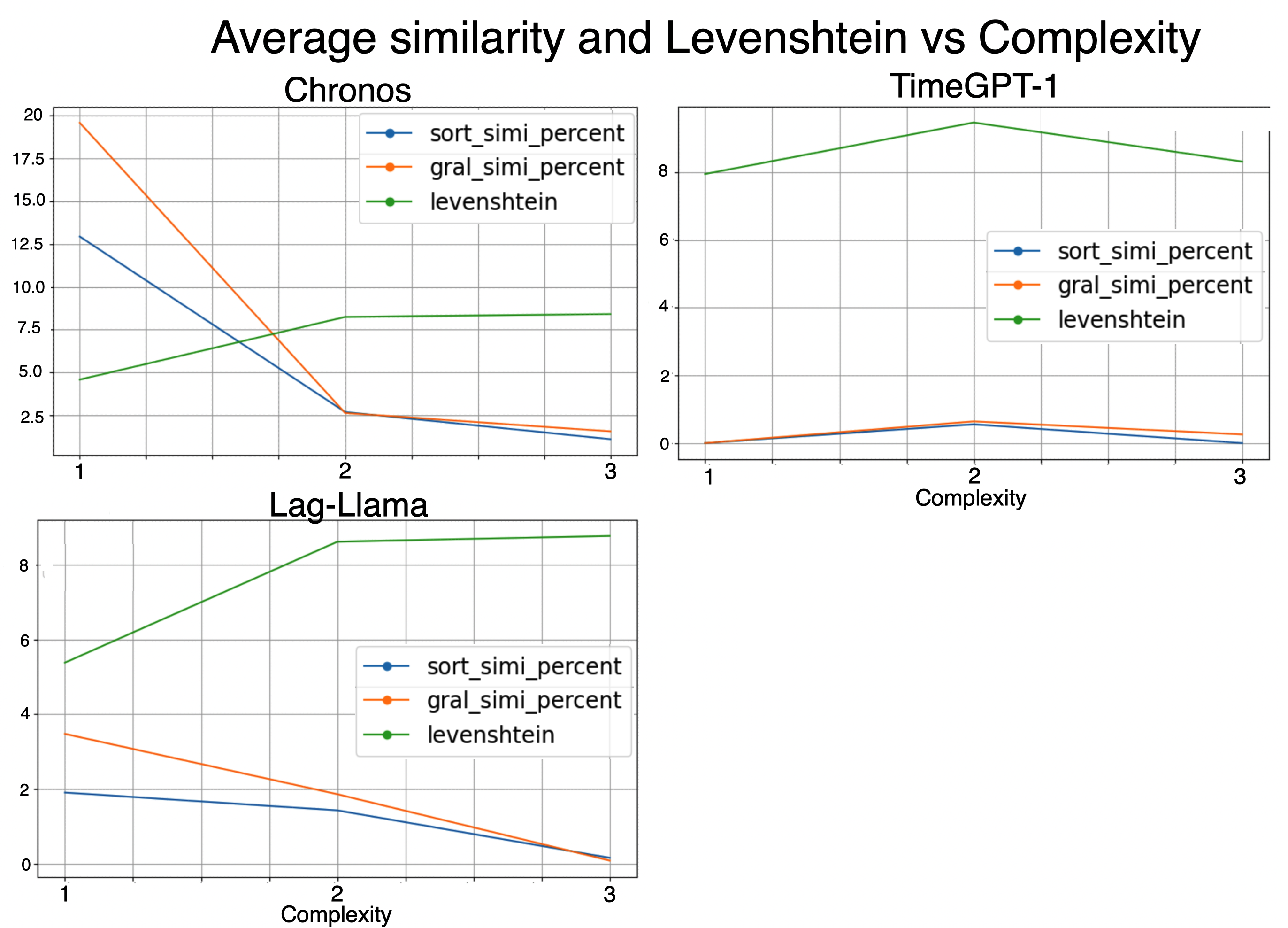
Figure 1: Similarity over predictions with Chronos, TimeGPT-1 and lag-llama. Methods and descriptions in the Supp. Inf.

We split our sequences into several segments, using the models described to predict the remaining portions, which correspond to 10%, 25%, 50%, and 75% of the sequence. This approach divided the sequence into a ‘root’ and a ’target’. For instance, given the sequence [1, 2, 3, 4, 5, 6, 7, 8, 9, 10] and a prediction of 25%, the ’root’ (the context provided to the prediction model) would be [1, 2, 3, 4, 5, 6, 7, 8], with the ’target’ [9, 10] expected to be predicted. An asymptotic distribution of test results $\varphi_{1},\ldots,\varphi_{n}$ for growing $n$ where $|s|=n$ should provide some insight into the generalisation of the capabilities of the LLMs to scale their reported abilities, if any.

We used three methods to measure the accuracy of the predicted target:

1. Sort similarity: This measures how many elements in the target sequence were predicted correctly, with their order being considered.

2. General similarity: This measures the correctness of predicted elements, without considering their order.

3. Levenshtein: This measures the Levenshtein distance between the expected and predicted sequences after converting them to strings.

5 Results

5.1 Next-digit Prediction Task with Binary and Non-binary Sequences

The objective of this experiment is to compare a fundamental characteristic of LLMs, that is, the prediction of the next token, with the power of understanding and then predicting approached through Algorithmic Probability Theory. This test, in particular, is inspired by  [74], which focuses on using Turing machines to approximate algorithmic complexity for short binary strings as a measure of algorithmic complexity as a means to explore fundamental principles of information and computational complexity, providing insights into the minimal description length of a string, an essential concept in understanding randomness and structured data.

We tasked Large Language Models (LLMs) specializing in time series prediction with predicting the final digit of both non-binary sequences and binary sequences, the latter of which were categorised as either random or “climber" sequences. The results of the experiment involving binary sequences are presented in Figure 2.

As shown in Figure 2, in the case of simple “climbers”, Lag-Llama achieved the best performance, with 70% precision, while TimeGPT–1 and Chronos barely reached 50% precision. However, for random sequences, which are considered highly complex, all models performed similarly, showing limited predictive power. This outcome suggests that, given the binary nature of the sequences, the models had a 50% chance of success, effectively reducing the task to guessing. These findings align with broader research that indicates that LLM models do not effectively capture sequential dependencies or complex patterns inherent in time series data. As highlighted by Tan et al. [75], despite their computational intensity, LLMs often fail to outperform simpler models, particularly when there is high complexity or randomness in the data.

A comparable analysis was conducted using LLMs specialised in time-series data, using non-binary sequences of increasing complexity. In this test, a specific percentage of the final numbers in each sequence was required to be predicted. Three distinct metrics were utilised: general similarity, sort similarity, and the Levenshtein distance (refer to the section  4.4.2 for its definition). Figure 1 presents the results, where sort similarity and general similarity exhibit closely aligned trends. This indicates that the predictive accuracy of LLM models, even when fine-tuned for numerical series, diminishes as the complexity of the sequences increases. The resemblance between sort similarity and general similarity implies that while predictions may include some of the expected numbers, their correct order remains equally critical and may not always be achieved.

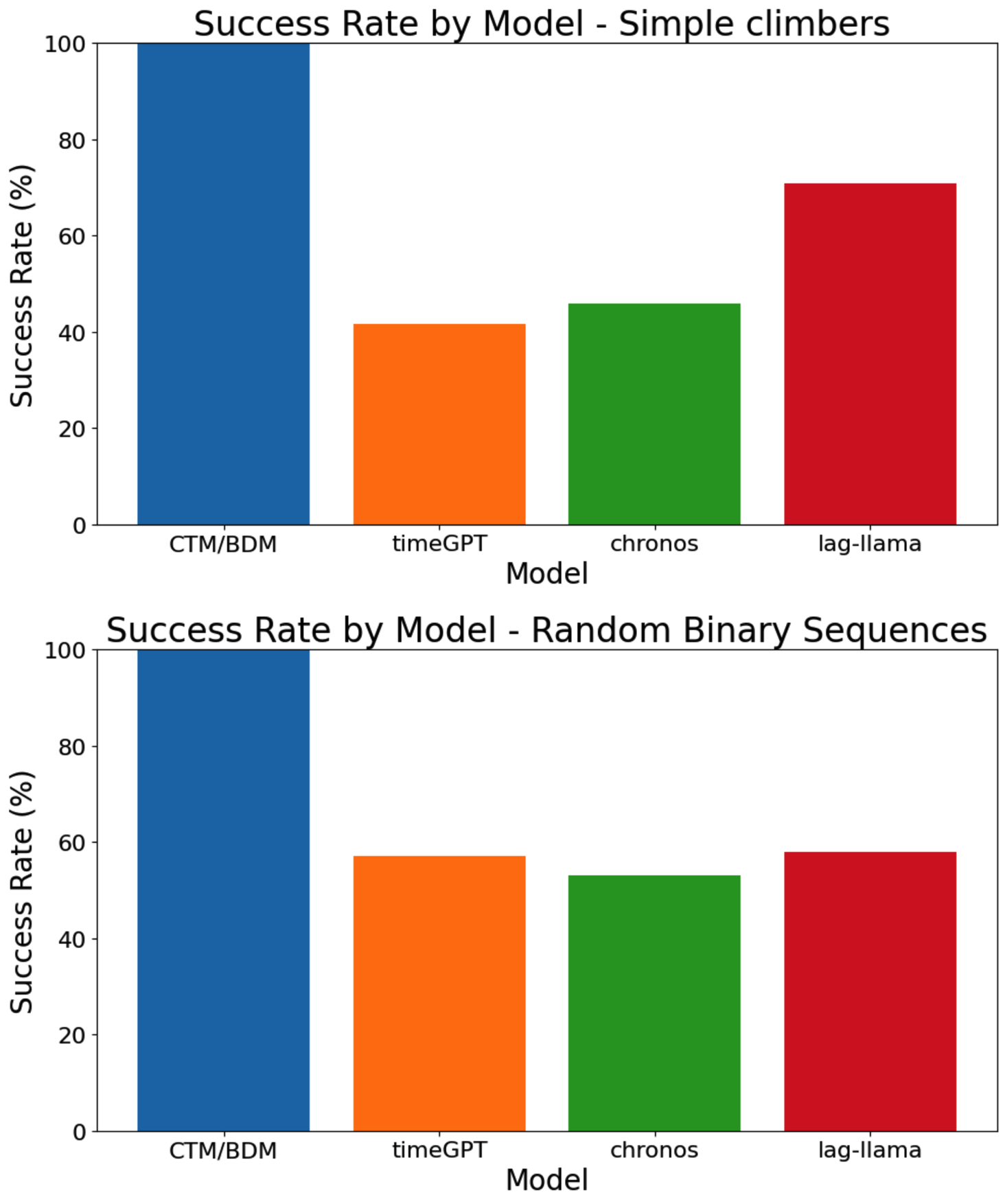
Figure 2: Percentage of accuracy on binary climbers and random binary sequences by LLM models specialising in time series prediction compared with BDM. That climbers (up) where better predicted is expected from models that are able to intrinsically characterise and better predict simpler sequences. That TimeGPT performed better for random sequences than the other LLM models is a surprise.

This observation is corroborated by the findings from the Levenshtein distance metric, which quantifies the minimum number of single-character edits (insertions, deletions, or substitutions) required to transform one sequence into another. As the complexity of the sequences rises, so does the Levenshtein distance, further confirming that predictive accuracy deteriorates with increasing complexity.

Figure 3 shows an increase in complexity as was expected given the design of each group of generated sequences. The plot suggests that BDM can capture (and can generate) better complexity and randomness, since its values increase more consistently as complexity increases, unlike other measures. Shannon-entropy-based measures (and cognates) can account for statistical randomness only. Compression algorithms, for example, decrease as complexity increases, becoming more difficult to find regularities and increasing compression length as a function of complexity growth.

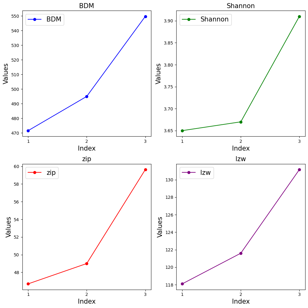
Figure 3: Quantitative Agreement of Monotonic Sequence Increase of Complexity: Comparison of BDM, Shannon Entropy, average length of Zip and LZW over the time series generated to test LLMs. Sequences chosen for each complexity class follow a pattern of increasing complexity in all cases, according to both statistical and algorithmic measures, and are used to build the testing sets, divided into three complexity groups, against which LLMs will be assessed.

5.2 Free-form Generation Task with Non-binary Sequences

A subsequent analysis focused on the free-form test, where Large Language Models (LLMs) were given complete freedom to generate any model or formula capable of producing target sequences of increasing complexity.

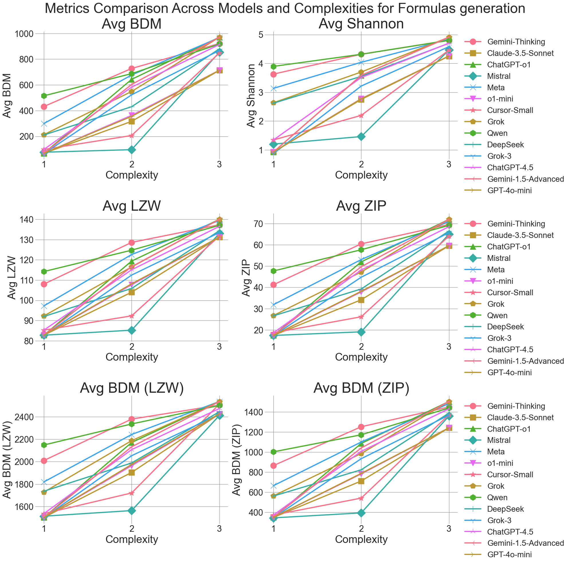
Figure 7: Complexity measures in the free-form test. LLM answers follow the theoretical expectation. For increasingly complex sequences, we see a decreasing number of compressed answers (or any answers at all) when LLMs are asked to produce a generating mechanism (such as a formula).

Figure 7 shows the plots of complexity-related metrics for the models and formulas generated by LLMs used in this research. The metrics evaluated include the length of the LZW-compressed model, the length of the ZIP-compressed model, the BDM (Block Decomposition Method) of both the uncompressed model and its LZW and ZIP-compressed forms, and the Shannon entropy of the model.

The plots reveal a clear positive correlation between model complexity and the metric values as the complexity of the target numerical sequence increases. Specifically, as the complexity of the sequence grows, the length of both LZW and ZIP-compressed representations increases, suggesting that the LLM-generated models become larger and less compressible. This indicates that the models provided by the LLMs become unable to compress and then to understand the logic behind sequences, giving as a result the sequence itself.

The BDM values (for the raw, LZW, and ZIP models) also exhibit an incremental trend, further supporting the observation that the LLMs generate less structured models when faced with more intricate sequences. Additionally, the Shannon entropy values rise with complexity, highlighting the increase in unpredictability or information content within the models as they attempt to approximate more complex patterns.

These findings suggest that the LLMs struggle to produce compact or efficient models as the complexity of the target sequence increases. The uncompressed models generated by the LLMs become longer and less structured, as indicated by the rise in all metrics. This reflects a limitation in the LLMs’ ability to discover or generate concise, elegant models for more complex sequences. Instead of producing simpler, more generalisable formulas, the LLMs resort to more convoluted representations, indicating a lack of sophistication in their capacity to identify or generate models that optimally balance complexity and brevity.

5.2.1 Emergent abilities

Another experiment aimed to evaluate characteristics recently attributed to large language models (LLMs), particularly their so-called emergent abilities, which include innovation, discovery, and improvement. These attributes have been claimed to enable LLMs to perform at levels comparable to the human top 1% in fluency and originality, as suggested by Zhao et al. in their assessment of creativity in artificial intelligence systems [76].

The experiment tested these claims by challenging LLMs to generate multiple, diverse approaches to reproducing non-binary sequences of varying complexity. The underlying rationale was that originality often stems from the ability to perceive problems in new, unexpected ways. Thus, the test focused on measuring the variety and creativity of outputs, as well as the models’ capacity to discover innovative or unconventional solutions.

Two distinct tasks were designed for this evaluation. In the first, models were asked to create any type of formula or mathematical model capable of replicating the target sequences. In the second, models were tasked with writing Python scripts to achieve the same goal. By incorporating these variations, the experiment sought to assess the models’ adaptability, computational reasoning, and creative potential across different problem-solving paradigms.

The results are shown in Figure 4 and Figure 5 where the following classification of cases was used:

1. Known Sequences: using standard algorithms such as Fibonacci or primes.

2. Pure Math: using mathematical operations without predefined sequence knowledge.

3. Not Found: inability to produce outputs.

4. Print Scripts: (only for script generation) trivial solutions directly printing the target sequence.

When it came to the production of different models or formula tests, while Gemini, Claude-3.5-Sonnet, and ChatGPT-1o performed relatively well, they ultimately shared the same core limitations as other models. In contrast, Meta and Mistral consistently underperformed, exposing disparities in baseline capabilities among LLMs.

5.3 Code Generation Task with Non-binary Sequences

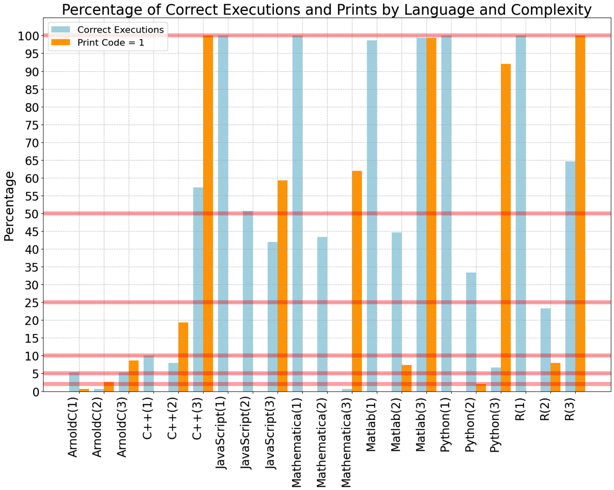
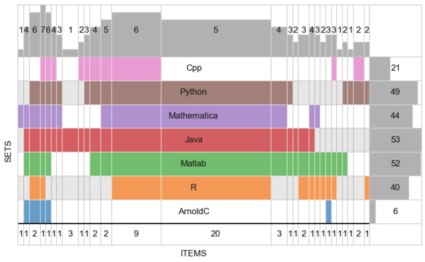
Figure 8: Top: Distribution of correct and print cases by language and complexity produced by ChatGPT-4. The results show an inversely proportional number of correct answers to sequences’ complexity increase, and a proportionally direct trend for simplistic print codes, both conforming with the expectation that higher complexity would retrieve fewer correct code evaluations and more trivial programs of type ‘print’, with a few exceptions, most likely as a result of examples found in the LLM training set. Bottom: Distribution of correct answers for ChatGPT-4. The upper section shows the number of scripts in different programming languages that reproduce the target sequences indicated below. The right section shows the total scripts by language successfully reproducing target sequences.This distribution highlights a subset of well-documented sequences accurately replicated by LLMs, with failures attributed to insufficient examples rather than language choice or understanding.

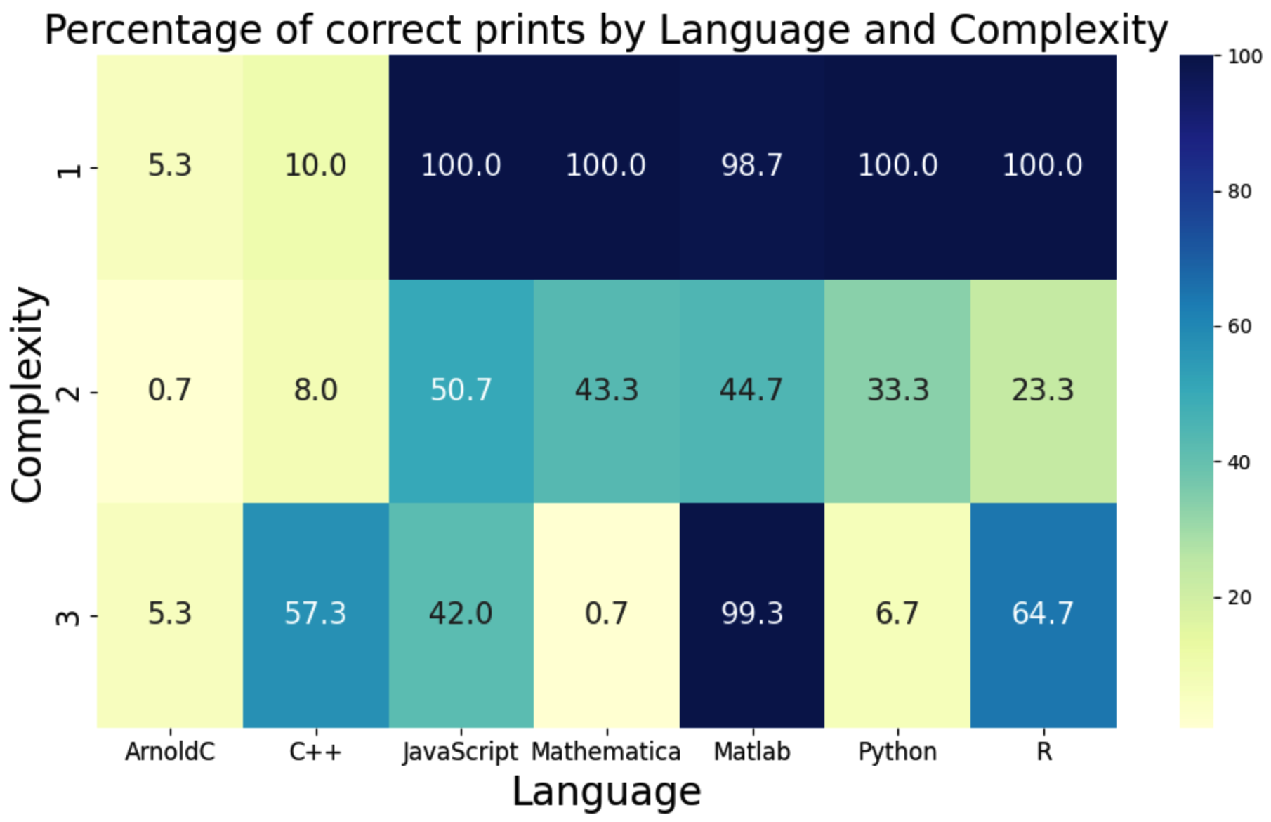
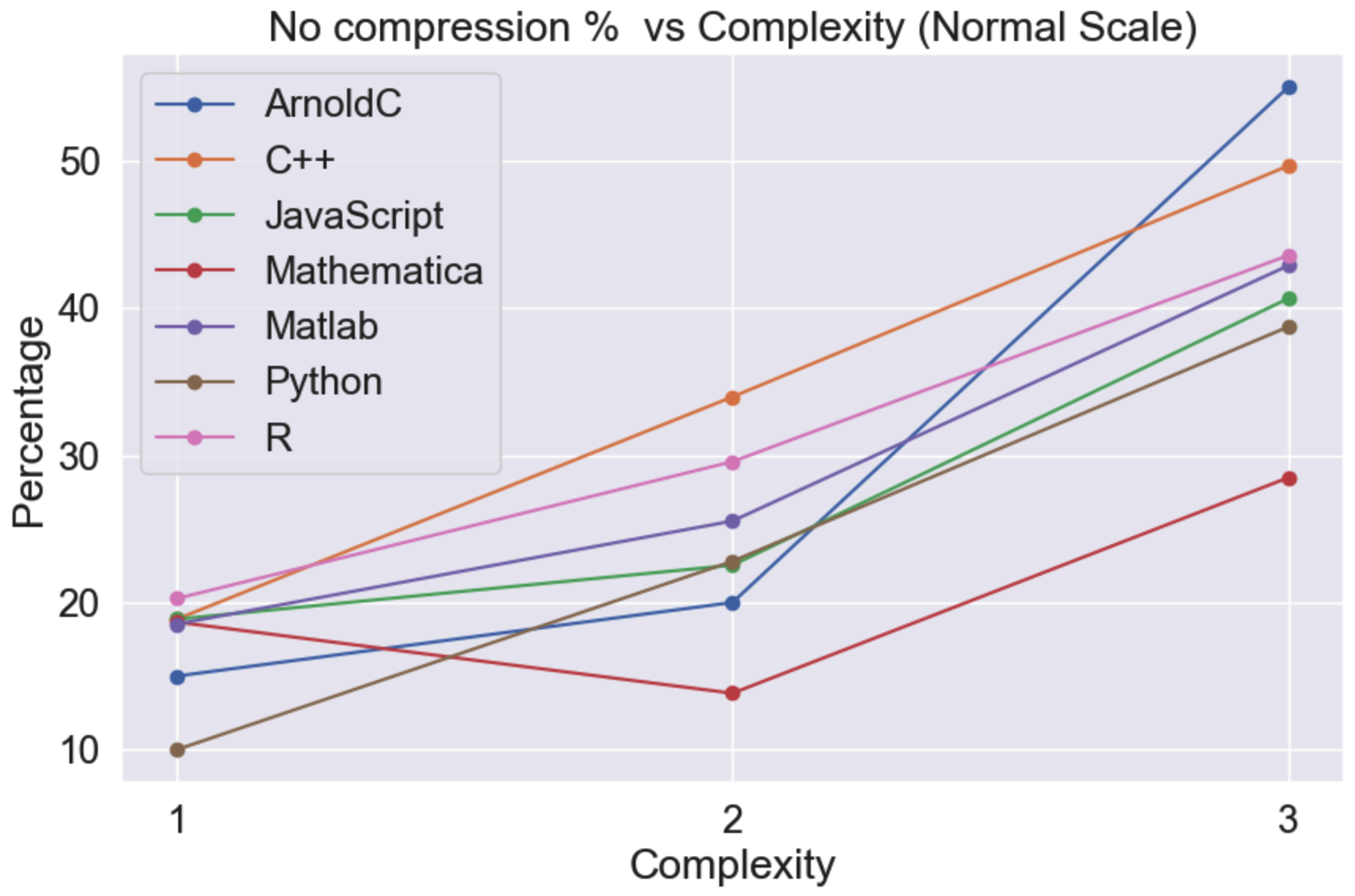
Figure 9: Top: Print cases by language and complexity for ChatGPT 4. Bottom: No compression percentage in original answers from ChatGPT 4.

For this experiment, one of the main metrics we measured was accuracy, which refers to the proportion of programs in different programming languages generated by ChatGPT that, after compilation and/or execution, produce the target sequence of digits. Figure 8 (top) shows that correct programs are more common at the lowest levels of complexity, with some minor exceptions. Figure 9 (top), on the other hand, shows the distribution of print cases by language and complexity level. They support the earlier observation that correctness in many instances is linked to a lack of compression.

Figure 8 in the Sup Inf. (bottom) shows the distribution of correct instances by sequence and by programming language generated by ChatGPT. The different programming languages are shown in coloured rows. On the right-hand side, the percentage of correct instances. At the top, the number of programming languages that overlap or solve the same problems correctly and, at the bottom, the extent of the overlap. For example, 5 languages solve the same 20 of 120 problems.

According to the results ( 8 top), the vast majority of correct cases are print failing to compress the sequences. This indicates that in most instances where the system correctly identifies a sequence, it does so by simply outputting the sequence as is, without any attempt at compression.

A second test performed to evaluate compression was based on the no-compression percentage. According to this metric, a compressed–and therefore, comprehended–sequence could be expressed as a general (and ideally short) program. Print cases are considered here to have 100% non-compression, since they involve displaying the original sequence as is, which in our test is synonymous with not understanding the sequence.

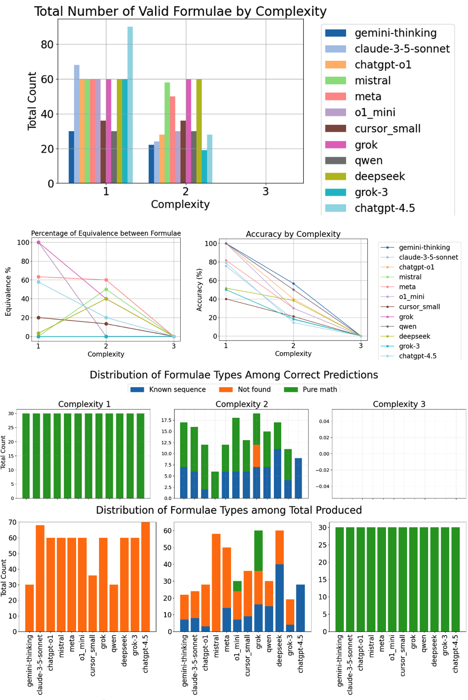
Figure 4: Analysis of formulae generation for numerical sequences of increasing complexity. Top: Total number of valid generated formulae, where valid stands for different to ‘Not found’ response. Middle: Percentage of equivalence (output similarity among generated formulae) and accuracy (correct replication of target numeric sequences). Bottom: Distribution of formula types among accurate and total responses. The results highlight a direct correlation between sequence complexity and the model’s inability to generalise. Notably, the limitations of LLMs are particularly evident in contexts allowing complete freedom to find diverse yet correct solutions, underscoring an absence of creativity and genuine understanding, attributes often mistakenly attributed to these models [76].The newest version of ChatGPT–o1, Grok and Gemini performed worse than its preview version (see Sup. Inf).

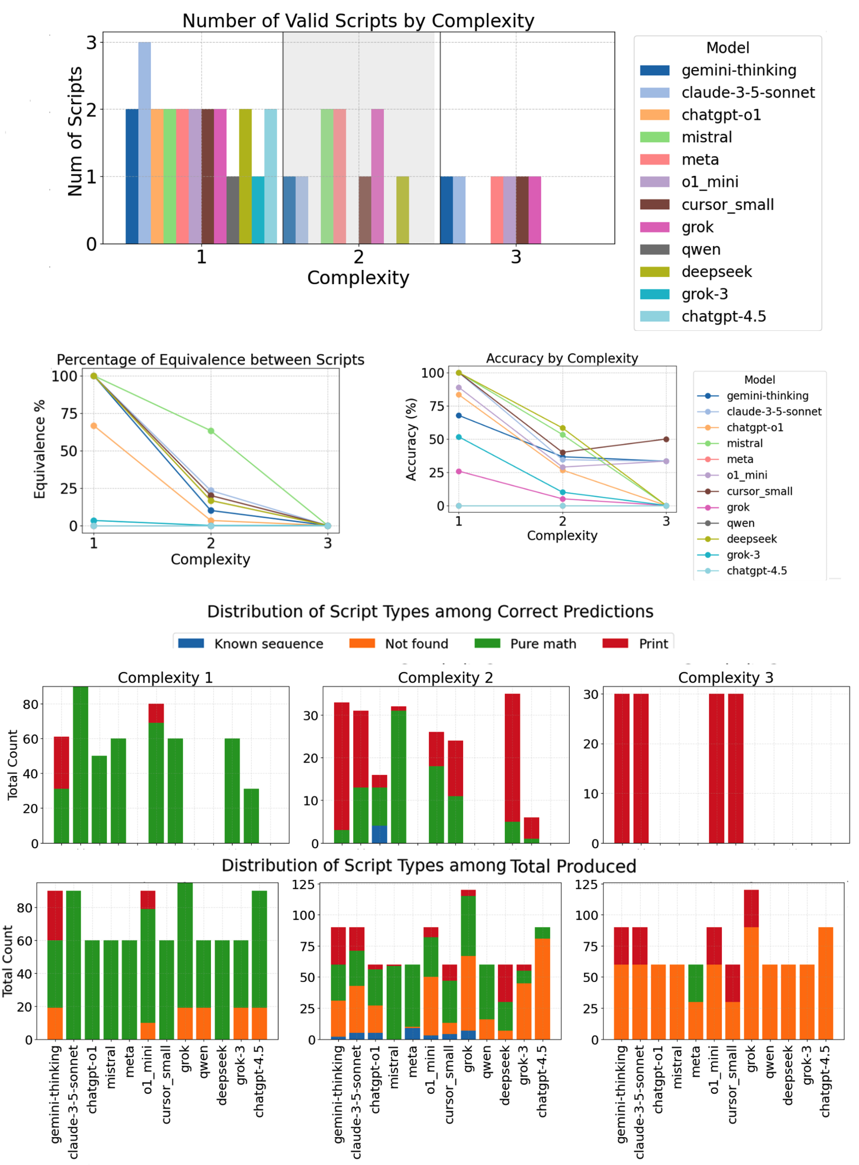
Figure 5: Analysis of Python script generation for numerical sequences of increasing complexity. Top: Total number of scripts generated with valid results. Middle: Percentage of equivalence (output similarity among generated scripts) and accuracy (correct replication of target numeric sequences). Bottom: Distribution of script types among accurate and total responses. The findings challenge the presumed ability of LLMs to outperform humans in solving well-defined yet complex tasks. While high equivalence and some capacity for coherent solutions are observed at higher complexities, low accuracy highlights significant limitations. Despite extensive training in Python, the results confirm that without similar examples in the training dataset, it becomes extremely difficult–if not impossible–for LLMs to deduce solutions or generate multiple valid answers for the same problem. The newest version of ChatGPT–o1, Grok and Gemini performed worse than its preview version (see Sup. Inf).

Figure 9 (bottom) shows how no-compression generally increases with complexity, except for Mathematica, where the no-compression percentage is lower at complexity level 2 than at level 1. This happened because Mathematica has the capacity to computationally replicate several well-studied and known sequences of numbers. This capacity leads to shorter code at complexity level 2. However, at complexity level 3 the trend aligns with other languages, showing direct proportionality between complexity and no-compression.

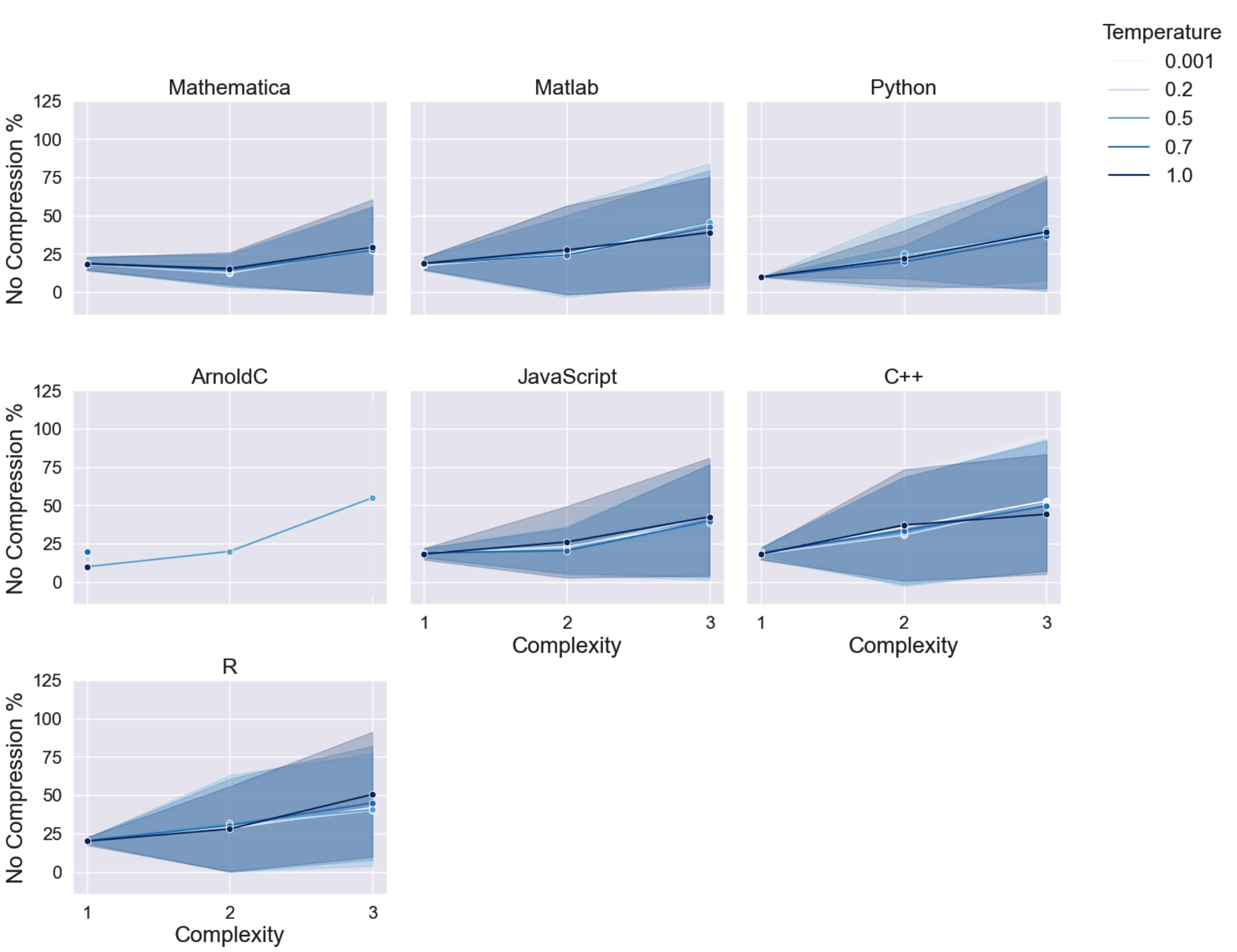
Figure 10: Complexity vs no compression and variation of temperature parameter showing robustness of results independent of controlled noise, where 1 is the typical LLM balance between ‘precision’ or repeatability and ‘creativity’ as defined by each LLM version.

Another analysis addresses the influence of the temperature parameter on the production of code to generate specific numeric sequences. In Figure 10, the average percentage of no compression by language, and across the different values of temperature used during the experiment is shown. This plot shows the shaded area representing the confidence tolerance over the average of no compression along the different values of complexity.

The trends in the percentage of no-compression across all temperature values are nearly identical, as are the shapes of the confidence intervals. The temperature value used to generate the code does not affect the result, indicating that the temperature does not have an impact on this experiment. It is worth mentioning the ArnoldC case, where in fact there were not many correct cases, making it difficult to calculate a confidence interval.

6 SuperARC-seq

Based on the previous experiments, it is possible to characterise one test directly related to the SuperARC framework: the SuperARC-seq. The objective of this test is to quantify intelligence and related cognitive capacities, specifically, reasoning and comprehension, drawing inspiration from the work in [74] and the theoretical and empirical studies here introduced. As mentioned, this test is grounded in one of the fundamental cognitive tasks: recognising patterns and evaluating the complexity of finite sequences, which inherently requires a level of understanding in order to provide a meaningful explanation. In our experiment, we generated short binary sequences and tasked several advanced LLMs with deriving a formula for each sequence capable of reproducing the target sequence.

We classified the correct answers provided by the LLMs into three types:

1. Prints: The model simply reproduced the target sequence without any attempt to encode or express it logically. This response type reflects a failure to abstract or deduce any underlying pattern, simply outputting the sequence as is.

2. Ordinal: The model provided a mapping based on the indices where “1”s occur in the sequence. This response reflects an attempt by the model to analyse and map some logical structure to the sequence, making it more valuable than simply reproducing it verbatim.

3. Non-Both: These responses avoided both simple reproduction and ordinal mapping, reflecting a more sophisticated approach to understanding and encoding the pattern. Such responses are the most valuable as they imply a deeper analysis and potentially creative logic to represent the sequence.

Thus, from these three types of correct results (i.e., the reconstructed sequence matches exactly the original one), we have four different classes of results: Correct & Non-Prints & Non-Ordinal; Correct & Ordinal; Correct & Prints; and Incorrect.

For any given tested model, the percentages of results belonging to each group can be combined as a vector of results, $\rho=[\%_{c,np,no},\%_{c,o},\%_{c,p},\%_{i}]$, such that $\sum\rho_{i}=1$ as the percentages will be represented in the range [0,1] to resemble probabilities. We know, beforehand, that the best performing model would be one with $\rho_{best}=[1,0,0,0]$. Thus, a first possible test would be to check the difference between correct and incorrect percentages.

$$\varphi_{a}=\sum_{i=1}^{3}\rho_{i}-\rho_{4},$$ (1)

which would range from -1 to 1 for models that are not able to reproduce any sequence to models which perfectly reconstruct the sequences, respectively. However, this only accounts for the ability of LLMs to reproduce the initial sequence (planning) but not for their compression capabilities. To account for the latter, let us assume that the best possible algorithm for each element of the data set is $\mathcal{B}_{k,j}$, such that $\mathcal{B}_{k,j}()=D_{k,encoded}[j]$, and here the algorithm does not have a particular input, similar to the definition of algorithmic complexity. Thus:

$$K(D_{k,encoded}[j])=K(\mathcal{B}_{k,j}())\leq K(\mathcal{B}_{k,j})$$ (2)

due to the information non-increase theorem and to the fact that no inputs were used in the function. In addition, it is clear that $K(\mathcal{B}_{k,j})\leq K(R_{k,j})$ since $\mathcal{B}_{k,j}$ is the shortest possible programme to reproduce $D_{k,encoded}[j]$. Thus, from equation 2:

$$K(D_{k,encoded}[j])\leq K(R_{k,j})$$ (3)

This suggests that the ratio $K(D_{k,encoded}[j])/K(R_{k,j})\leq 1$ could be used as a weight to indicate how well the model achieves compression and comprehension, with the best possible value equal to 1 representing a perfect ratio scenario. Since we have several algorithms classified under each of the four types (according to their structure), instead of using the individual ratios, we shall use the harmonic mean per type, defined as:

$$\delta_{k}=\frac{n_{k}}{\displaystyle\sum_{j=1}^{n_{k}}\frac{K(R_{k,j})}{K(D_{k,encoded}[j])}}\text{ for }R_{k,j}\text{ of type }k,$$ (4)

where $n_{k}$ represents the number of algorithms that are of type $k$. If we include $m$ sequences in the test, for example, $n_{k}=m\rho_{k}$. Thus, an updated version of the test is:

$$\varphi_{b}=\sum_{i=1}^{3}\delta_{i}\rho_{i}-\rho_{4}.$$ (5)

Deliberately, instead of calculating the harmonic average of complexity ratios for formulas of incorrect type ($\delta_{4}$), we penalise the test the most and set the weight $\delta_{4}$ to -1. Besides, we want to privilege models that do not simply copy or provide ordinal mappings of the input sequences. Thus we can attribute higher weights to types that are correct and do not copy nor print the results. We also want to give more weight to programs that provide ordinal mappings when compared to print cases. Then, considering a power-law weighting strategy, the final test metric is:

$$\varphi=\delta_{1}\rho_{1}+\frac{\delta_{2}\rho_{2}}{2}+\frac{\delta_{3}\rho_{3}}{4}-\rho_{4}.$$ (6)

It can be seen that $\varphi\in[-1,1]$ encompasses different behaviours. For example, $\varphi\in[0,0.25]$ if only print-type models are outputted. Also, $\varphi\in[0,0.5]$ if only ordinal-like formulas are created. Finally, $\varphi\in[0,1]$ in cases where the LLMs create formulas that are always correct, do not copy nor create ordinal mappings. The ranges will be populated with varying compression levels corresponding to the algorithms obtained. The test performance results for each model are calculated using equation 6 for $\mathcal{T}$ in Algorithm 1.

There are some possible variations for the test metric in equation 6. For example, some sort of Bayesian approach could be used to consider that the elements of $\rho$ are not constants, but random variables which could account for the number of different correct/incorrect answers for the same input sequence. In this way, the multiplicity of possible generators is taken into account, better capturing the concept of algorithmic probability, and the output of the test would be a random variable instead. However, LLMs hardly produced even one correct answer, therefore we kept the formula simple.

As described, equation 6 tests for two features, compression via non-print computer programs and non-ordinal mathematical formulas to the input sequence, and prediction, by running all programs and all formulas to match each sequence digit, and penalising them when they did not represent an actual compressed model that generated a possible new digit of the sequence when run in reverse, i.e. when ‘decompressed’. The test formula assigns greater importance to correct cases that are not solutions of the type ‘print($s$)’ where $s$ is the sequence for which the AI system is asked for a model, given that a print model does not allow generalisation by prediction through simulation, as running a print command will only print up to the last digit. The same is true for what we call ‘ordinals‘, which is simply indicating the index of the non-zero non-one element in the binary sequence, meaning that, together with the ‘print’ case, the system failed in its attempts at abstracting features of the object. Finally, the formula punishes ordinal and print answers in a weighted fashion. The best performer can only reach a $\varphi$ of 1 while the lowest value is -1.

6.1 Applying SuperARC-seq

The results of the LLM classification tested by applying this test according to the formula are shown in Table 1 and summarised in Figure 6. As shown in Table 1 and Figure 6, CTM/BDM would achieve perfect scores in all categories, consistently avoiding trivial responses and providing accurate formulas. By design, this model clearly excels in abstract feature recognition, outperforming all other models at prediction, which we claim is key to planning. CTM/BDM actually produces a set of possible generative models (computer programs) that, when run in reverse in what would be the uncompressing process, produce new elements to test against the observation, thus updating and producing new possible outcomes. These models are also hypotheses that do suggest whether a sequence is random or not, rather than looking for such a sequence in the training set or a combination thereof and failing for those not found in the distribution.

Model $\rho_{1}$ $\rho_{2}$ $\rho_{3}$ $\rho_{4}$ $\delta_{1}$ $\delta_{2}$ $\delta_{3}$ $\varphi$ ASI (AIXI/BDM/CTM) $1.000$ $0.000$ $0.000$ $0.000$ $1.000$ $0.000$ $1.000$ $1.000$ mistral $0.670$ $0.000$ $1.000$ $0.180$ $1.553$ $0.000$ $0.116$ $0.100$ gpt_4o_mini $0.390$ $0.000$ $1.460$ $0.000$ $1.551$ $0.000$ $0.160$ $0.090$ claude_3.7 $0.400$ $0.810$ $0.320$ $0.320$ $1.060$ $0.032$ $0.313$ $0.067$ chatgpt_4.5 $0.440$ $1.000$ $0.000$ $0.410$ $1.008$ $0.030$ $0.000$ $0.063$ cursor_small $0.490$ $0.000$ $1.000$ $0.360$ $0.691$ $0.000$ $0.141$ $0.061$ deepseek $0.590$ $0.000$ $1.000$ $0.260$ $0.345$ $0.000$ $0.116$ $0.059$ qwen $0.590$ $0.000$ $1.000$ $0.260$ $0.204$ $0.000$ $0.116$ $0.056$ o1_mini $0.520$ $0.640$ $0.140$ $0.550$ $0.595$ $0.058$ $0.224$ $0.051$ gemini $0.410$ $0.000$ $1.000$ $0.440$ $0.255$ $0.000$ $0.141$ $0.047$ gpt_4o $0.410$ $0.000$ $0.360$ $1.080$ $1.384$ $0.000$ $0.313$ $0.039$ grok_3 $0.480$ $0.020$ $0.000$ $1.350$ $1.027$ $0.424$ $0.000$ $0.023$ meta $0.670$ $0.000$ $0.000$ $1.180$ $0.285$ $0.000$ $0.000$ $0.017$ claude_3.5 $0.140$ $0.460$ $0.000$ $1.250$ $0.129$ $0.116$ $0.000$ $0.007$ o1_preview $0.010$ $0.290$ $0.140$ $1.410$ $2.493$ $0.048$ $0.224$ $0.000$

Table 1: Numerical benchmark ranking of popular frontier models publicly available against ASI from methods like AIXI [77] or neuro-symbolic approach such as CTM/BDM [69, 20].

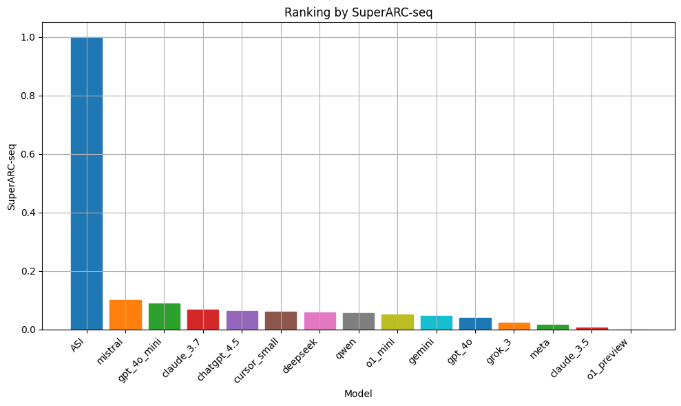
Figure 6: Renormalised benchmarking plot from Table 1 showing how most frontier models are close to each other in their performance under this test and far from AGI or ASI goals according to this test. ASI would be able to distinguish simpler from complex sequences and generate predictive models for each accordingly, as AIXI [11] or CTM/BDM would do [20, 69] as instantiations of universal AI hence ASI. Today, LLMs only produce or retrieve models for sequences that were seen and found in their original training sets, given that increasing the sequences’ lengths impacts the LLM performance in identifying the sequence, hence indicating sequences are not recognised from first principles but from simplistic pattern matching.

These findings indicate that LLMs perform well when there are discernible patterns in the data, but struggle with randomness, failing to capture complexity in an algorithmic sense. In contrast, Algorithmic Probability Theory can accurately predict (rather than guess) the sequence, regardless of the string’s complexity. These results demonstrate that the algorithmic-complexity approach effectively approximates the minimal description length of information, identifying the shortest algorithm capable of generating a given sequence.

Despite being the top-ranked LLM models, all LLMs only provided exact copies of the inputs, which achieved correct results at the cost of no abstraction and comprehension at all. The o1–mini and o1–preview LLM versions produced several incorrect formulas and ordered-seeming responses, indicating a lack of pattern recognition beyond basic sequence reproduction. GPT-4o and Meta got all the formulas wrong.

Unlike standard LLMs that predict the next tokens in text, CTM/BDM finds the mechanistic generators of the sequence by a combination of symbolic and statistical pattern matching algorithms, which allows it to derive concise models that can then run in reverse to match each digit and produce new ones, hence allowing prediction and planning by picking the most likely among a set of possible models based on the algorithmic probability of the model (how short and how often the same model was found to produce the same sequence).

7 Conclusions

Previously, we showed that aspects of human [2, 78] and animal [3]) cognition and intelliegnce could be characterised, and aspects of their behaviour reproduced, in terms of algorithmic probability tools and metrics that we have also suggested for artificial systems, including robots [4]. Here, we tested these ideas and proposed a new quantitative metric based on the principles of algorithmic information theory related to recursive compression (as opposed to statistical) and prediction in application to LLMs that are believed or have been proposed to be capable of approaching AGI and Superintelligence.

Another problem in LLM testing is benchmarking contamination; this is the targeted optimisation over or leakage of the answers to a test. The open-ended nature of this test is intended to counteract this problem of benchmarking contamination and cheating. We have introduced and demonstrated that recursive compression can quantify model abstraction and prediction based on a new result and mathematical proof of equivalency between model compression and prediction applied to sequences based on Martingales, without resorting to Martin-Löf randomness tests (see Sup. Inf.). By incorporating and exploiting the formal equivalence between prediction and recursive compression into an intelligence test framework, we align the assessment of intelligence with fundamental computational principles. An agent’s ability to abstract information through feature selection and model compression reflects its capacity to identify and utilise patterns within data. Similarly, its planning and prediction skills demonstrate its ability to anticipate future events based on these patterns.

Our investigation of frontier models, framed within the algorithmic complexity paradigm, yields several key insights about the models’ comprehension capabilities. Most of the models demonstrate poor accuracy in replicating and predicting even simple and recursively generated sequences beyond clearly memorisation results from the training distribution (such as sequence labelling). The vast majority of the correct answers turned out to be simple print statements of the numerical sequences themselves rather than any code or model indicating any sign of understanding or pattern recognition.

These conclusions are reinforced by the model’s explicit dependency on specific programming languages for correctness or on well-studied and documented series of numbers. In other words, if there are not enough implementations available in a specific programming language for the model to learn from, or even specific methods of mathematical analysis over specific numerical sequences, LLMs failed to produce the correct answer. Rather, considering the most popular and widely used languages, LLMs do not demonstrate understanding, but instead rely on selecting from an abundance of previously seen cases.

We have previously shown how optimal prediction can be achieved by using BDM as a testing tool but not as the model generator. We have also shown how BDM can be used in the opposite fashion, not only as a testing tool for intelligence, but as a model generator [20, 79, 19], as an approach to optimal inference through the Coding Theorem Method and Algorithmic Probability [69, 80, 81]. While CTM can be seen as a brute force apprach to a giant lookup table of micro-programs to explain the data, BDM is not. BDM combines the algorithmic probability approximations produced by CTM but then stitches each most likely program for each piece back together according to valid laws of information theory in what constitutes a pure form of hybrid statistical and symbolic explanation, hence neurosymbolic. BDM, therefore, uses the two best inference theories currently available to science, one being the most used and overused in statistical Machine Learning (Shannon Entropy, with its limitations [82]), and one that has been neglected on the basis of uncomputability [83, 34]. BDM therefore always provides the best approximation and guarantees an estimation to finding the correct sequence of micro programs to the observation, providing a computable set of models for the explanandum.

While LLMs are impressive linguistic tools, LLMs were never designed to reason, infer or perform rationally beyond statistical alignment. We suspect that LLMs are too slowly moving towards symbolic computation like BDM, which transparently combines statistical pattern matching and causal inference. While the results may read negative, a positive reading is that there is still a lot of room for improvement despite claims of AI hitting a wall through a lack of data to feed an ever-increasing need. This means that an enhancement of nontrivial performance in agnostic abstraction and universal planning will likely be the result of symbolic computation and not of pure statistical memorisation.

Recursive compression and optimal prediction go hand in hand [30], but previous tests focused on particular subset features, even those designed to test human reasoning and human abstraction such as ARC [27].

We have reported that top-performing LLMs currently perform close to pure-copy solutions, with even advanced models struggling to produce correct model extraction and predictive results. These results would also imply a poor performance if LLMs in traditional tests of education as introduced by e.g. Bloom [84] in its education hierarchy for humans testing for new knowledge and synthesis generation test. The results confirm that current LLMs, while competent in pattern replication, lack critical elements associated with AGI and ASI. All LLM’s involved in this test showed dependence on predefined patterns. As complexity increased, models relied increasingly on trivial strategies, such as direct sequence printing or brute-force simplistic mathematical expressions. This highlights the LLMs’ inability to abstract or conceptualise novel solutions.

The level of equivalence says a lot about creativity in bringing about new knowledge. The high equivalence with greater complexity often reflected repetitive outputs rather than meaningful creativity. This tendency to revert to safe and redundant approaches underscores the models’ limited exploratory capabilities.

An inability to generalise can be detected. The steep decline in accuracy and functional outputs as complexity increased reveals that these models are heavily reliant on memorisation and predefined rules. They struggle to generalise knowledge or engage in higher-order problem solving.

The models’ outputs suggest strength in replication but a lack of adaptive and ‘inventive thinking’. The predominance of trivial or incorrect solutions demonstrates an inability to think ‘outside the box’ (as in if it had not been seen in the training distribution). This suggests that while LLMs can mimic comprehension through retrieval. pattern matching and Chain-of-Thought techniques, their capabilities remain bounded when tested against algorithmically complex sequences.

We have argued throughout this contribution–and it is distilled by our test for intelligence–that only semicomputable open-ended tests can be powerful enough to quantify the full extent of our conception of natural intelligence, human [2, 78], animal [3]) or artificial [4]. And that one lesson from LLMs is that we should dissociate language from intelligence, something Turing himself suggested with his imitation game [7].

And that the converse is also true, that only incorporating sufficiently powerful open-ended semi or uncomputable predicting generators, such as the methods explored (BDM running on CTM), may achieve Superintelligence by way (or not) of AGI. We have also argued that optimising for the features that our test captures will lead to Superintelligence.

Based on these results and first principles, when it comes to chatbots in the context of their claims about ‘reasoning’ capabilities and AGI/ASI, it is our belief that any AGI/ASI system will actually show more ‘difficulties’ in displaying human language capabilities if they actually mean the words they produce as opposed to emulate a coherent conversation as in current LLMs that perform so well in human languages out of the box as their main feature, with causality and meaning neglected.

We believe that this test has fundamental significance because it demonstrates that LLMs primarily rely on direct pattern matching, making it impossible for them to predict in even basic and well-defined scenarios in a meaningful way. This limitation is closely related to the phenomenon of hallucinations in LLMs, which reinforces the criticism that LLMs lack an internal model of the world to allow them to simulate possible future scenarios and pick the most likely for planning purposes. Instead, they statistically generate a scenario for each predictive challenge, where the LLM is forced to build a coherent answer without an underlying model representation or causal inference capability making claims about ‘reasoning’, reaching AGI, or heading toward Superintelligence, unfounded.

8 Code and Data Availability

Code and data generated for this work are available at https://github.com/AlgoDynLab/SuperintelligenceTest.

Supplementary Information

Further test context and future research

This first version of a test based on the SuperARC framework, hereby named SuperARC-seq, has its initial application related to studying sequences of integers with different complexity classes. Although this type of test has received some criticism for being suitable for static situations only (where the intelligent agent does not interact with the computable environment) [85], other frameworks and adaptations have been proposed [15]. In addition, sequence prediction as a pure prediction task resembles a subset of IQ tests [86] and it has been shown that there are some ML models which can excel at that [87] and break the test for next-generation LLMs (just like OpenAI’s o1 model did with the ARC challenge). Overall, it must be clear to the reader that the prediction task here considered is constrained by the computational complexity of the solution (thus it is not a mere sequence prediction task that could be naively solved with interpolation polynomials, for example). The prediction should consider previous examples and the most natural solution (here understood as the one with lowest complexity).

In order to further expand the application of the SuperARC framework, combining it with other tasks can be of great interest. For example, some tasks have been proposed to test LLMs with respect to the computational aspects of the learned compressed representation, as one of the subtests of the framework called “Beyond the Imitation Game: Quantifying and extrapolating the capabilities of language models”  [88], which evaluates the capability of language models to learn algorithmic concepts in a universal language (Turing-complete) under the perspective of machine teaching. In that case, using the concepts presented here, especially BDM as a benchmark and as a decision support tool (algorithm selection), could lead to even more powerful implementations of SuperARC. The same can be said about other frameworks such as DyVal [89], which considers the structural advantage of directed acyclic graphs to dynamically generate evaluation samples with controllable complexities. DyVal generates challenging evaluation sets on reasoning tasks that include mathematics, logical reasoning, and algorithm problems, and the latter can be considerably enhanced by AIT and the SuperARC framework. On the same subject, Kolmogorov-Test (KT) [90] explored an approach to intelligence testing through algorithmic complexity and compression, but while SuperARC and KT recognise compression as a fundamental aspect of intelligence, KT focuses specifically on the evaluation of code generation by LLMs. In particular, KT considers codes in Python, whereas SuperARC presents a broader intelligence test applicable to AGI and ASI, and compares it to a pure form of Neurosymbolic computation that can reach AGI and ASI. Combining some of the concepts behind KT with SuperARC, especially the use of CTM and BDM to estimate the algorithmic complexity of codes, could yield interesting applications of SuperARC. Despite these differences, both KL and SuperARC share common ground in their use of algorithmic complexity as a foundation for intelligence measurement. Both studies highlight the limitations of LLMs in achieving true intelligence, with KT focusing on their inability to generate optimal programs and SuperARC demonstrating their struggles with generalisation, planning, and abstraction.

Other implementations of SuperARC may involve the concept of conversational complexity  [91], defined as the algorithmic complexity of the user’s instruction sequence leading to a given response by LLMs. One possible approach is to use this as a proxy for intelligence, where more intelligent LLMs require user instructions with lower algorithmic complexity to achieve the expected results. In that case, LLMs would be understood as the Universal computing systems to which instructions (prompts) are submitted. This concept shifts the notion of ‘intelligence’ by focusing on the level of assistance an LLM needs to produce accurate outputs. Since LLMs often require extensive context, intelligence in this sense would be defined by their ability to accomplish more with fewer inputs (aligned with Occam’s razor). Using different prompts, like the Structured Chain-of-Thought Prompting for Code Generation proposed in  [73], can considerably increase the quality of LLMs outputs (particularly when the prediction task is carried out by running a code produced by the LLM), but conversational complexity would flag this prompt complexity increase, preventing LLMs from “cheating” on the test by leveraging better prompting techniques. Also, by exploring LLMs in their “original” text-like grammar, language-symbolic alternatives such as the one in GSM-Symbolic [92] could be combined with the SuperARC testing framework. In that case, by combining the symbolic prompt templates in GSM-Symbolic with SupeARC’s robust AIT framework, interesting metrics for measuring the reasoning capabilities of models could be obtained.

In order to make CTM/BDM useful for botchatting, it would need to invest resources to make it look mundane, almost reversing its super capabilities. An interesting analogy is to Borges Babel’s library, LLMs are like a version of its library or produced by all the possible random combinations (as in the original library), the recursive library as introduced in [30] is the version in which every book could only be recursively generated, one that was causally generated and does not include every possible permutation. If there is any filtering, it happens over a smaller set of only constructive sets, but every word in every book would be meant in the deepest way because it is all connected constructively to some common origin or common history.

8.0.1 Is the SuperARC a reasonable challenge?

An argument that could be made is that CTM is a brute-force approach to this problem, but it does not require nearly as many computational resources as the billions of dollars needed to train or run an LLM to start delivering complementary results to LLM pattern-matching that can materially improve their ‘understanding’ and predictive power. While CTM is indeed based on a brute force approach and is necessary to guarantee convergence to the purest form of ASI, BDM exploits CTM efficiently as a greedy algorithm by decomposing a problem into smaller pieces. This combination is therefore both powerful and efficient to some extent, leveraging the strengths of both sybolic and neural approaches.

We have proven that the worst-case performance of CTM/BDM is equivalent to a Shannon entropy estimation [69], on which most, if not all, loss functions and ML kernels are in some way or another based. Consequently, this means that CTM/BDM cannot perform worse than statistical Machine and Deep Learning methods–it can only improve performance from CTM, despite its computational expense, which remains significantly lower in practice than that of Deep Learning or LLMs today.

No credible argument in favour of Neural Networks’ efficiency, as opposed to allegedly brute-force approaches, can be made when considering, for example, self-driving cars requiring tens of millions of miles of driving to learn how to operate a car with questionable skills.

CTM may approach impracticality when dealing with high-complexity sequences, but this does not apply to sequences on which LLMs fail. Low- and medium-complexity sequences include the digits of the mathematical constant $\pi$, or prime numbers. LLms may identify prime numbers, yet they fails to generate programs in general other than direct ‘print’-like statements for even simple sequences–let alone more complex ones.

For example, if prompted for the next digit in an initial segment of $\pi$, the longer the sequence, the higher the error rate–even when the number is ‘identified’ as $\pi$. Rather than computing the digits using a formula, an LLM must search its training dataset for previously seen sequences and then attempt to reconstruct them. More often than not, this approach fails as the sequence length increases. Notably, however, our tests begin with very short strings, as brief as 11 to 20 digits, and yet LLMs perform poorly, rarely generating the correct computer program or formula that produces the sequence.

Additionally, another interpretation of this benchmark is that new models are not improving over time, strengthening the suspicion that LLMs may have reached a performance plateau [54]. This is due to their inability to generalise beyond specific cases found in their training data. In this paper, we suggest that optimising for the features that enable abstraction from a sequence and allow for next-symbol prediction is fundamental to model creation and planning, which, according to AI researchers and cognitive scientists, are key components in defining intelligence.

A positive perspective is that we propose methods to actually achieve Superintelligence, formally defined by Algorithmic Probability as the ultimate method of optimal inference, where for any computable question, the correct computable answer is retrieved.

Regarding objections to brute-force approaches, deep learning and LLMs currently appear far more resource-intensive, as seen in self-driving cars requiring hundreds of millions of miles of training before they are able to operate. The method we propose integrates LLM and Deep Learning technology (which relies on classical information theory, statistics, and certainty) with symbolic computation, a field already capable of narrow Superintelligence, as seen in arithmetic calculators and theorem provers.

We believe that optimising this relationship will ultimately lead to Superintelligence.

Equivalence between compression and prediction via Martingales

An infinite sequence (or equivalently, a real number) is denoted by $x=x_{1}x_{2}x_{3}\ldots$, where each $x_{i}\in\{0,1\}$. Let $x\upharpoonright_{n}$ the sequence of the first $n$ bits of the binary representation of $x$.

A (super)martingale function $d:\{0,1\}^{*}\rightarrow\mathbb{R}^{+}$ represents a betting strategy that satisfies the fairness conditions:

• $$d(\sigma)=\frac{d(\sigma 0)+d(\sigma 1)}{2}\text{, in the case of a martingale;}$$ (7)

• $$d(\sigma)\geq\frac{d(\sigma 0)+d(\sigma 1)}{2}\text{, in the case of a \emph{super}martingale.}$$ (8)

This conveys the idea that the expected capital after the next bet is either equal (for martingales) or is lost (for supermartingales) with respect to the previous capital.

A (super)martingale $d$ succeeds on a sequence $x$ if:

$$\limsup_{n\rightarrow\infty}d\left(x\upharpoonright_{n}\right)=\infty$$

This implies that the betting strategy can make an unbounded amount of money on $x$ at the asymptotic limit as the length of the initial segment of $x$ increases.

A martingale $d$ is (left) semicomputable if there is an algorithm that computably enumerates the left cuts of $d(\sigma)$ for any given string $\sigma$. Thus, if a semicomputable $d$ succeeds on a sequence $x$, this (super)martingale can be interpreted as revealing the existence of an algorithm that can computably enumerate a betting strategy that always increases its capital gains at the asymptotic limit as the length of the initial segment of $x$ increases. This holds even if eventually one loses expected capital in the next bit (as the supermartingale condition allows). The existence of such an enumerating algorithm guarantees that there is at least one asymptotically effective way of predicting the forthcoming bits in the infinite sequence $x$ so as to render the betting strategy successful as this process goes on.

Now, remember that an algorithmically random infinite sequence (or real number) $x$ is incompressible up to a fixed constant so that $K\left(x\upharpoonright_{n}\right)\geq n-\mathbf{O}(1)$, and the constant does not depend on $n$. Therefore, if $x$ is not algorithmic random, then for any $k$ and for any $n^{\prime}\geq 1$, there is $n\geq n^{\prime}$ such that $K\left(x\upharpoonright_{n}\right)<n-k$. In other words, $x$ is compressible (by more than a fixed value) infinitely often.

The notion of predictability conveyed by martingales should reflect the fact that in the case of an algorithmically random sequence, there would not exist an enumerating algorithm that guarantees that there is at least one asymptotically effective way of predicting the forthcoming bits in the infinite sequence $x$ so as to render the betting strategy successful as this process goes on. In summary, one should not expect to be able to devise a computably enumerable betting strategy that is successful on a perfectly random sequence. Indeed, the equivalence between (super)martingales and algorithmic randomness holds:

• If a sequence $x$ is not algorithmically random (i.e., it is compressible infinitely often), then there exists a semicomputable martingale that succeeds on $x$.

• Conversely, if there exists a semicomputable martingale that succeeds on $x$, then $x$ is not algorithmically random (i.e., it is compressible infinitely often).

Another equivalence between algorithmic randomness and the notion of predictability can be achieved from (stochastic or probabilistic) martingale processes which are defined upon real-valued random variables. In this case, one can demonstrate that an infinite sequence is algorithmic random iff no computable martingale process succeeds on it [25].

Usually, (super)martingales and randomness are demonstrated to be equivalent via proof- and measure-theoretic statistical (Martin-Löf) tests. A sequence is incompressible iff it does not pass on any ($\Sigma_{1}^{0}$) theoretic statistical test [25], thereby called (prefix) algorithmic random ($1$-random or $\mathbf{O}(1)$-$K$-random). It is important to remark that the triple equivalence between predictability (via martingales), statistical tests (via proof and measure theory), and compressibility (via algorithmic complexity) establishes one of the foundational results in the theory of algorithmic randomness and algorithmic information [25, 24].

In order to highlight the connection between predictability and compressibility, we introduce in the following a novel and alternative proof for the direct equivalence between compression and (successful computably enumerable) martingales.

As for algorithmic randomness deficiency [26], one can define a weaker notion of supermartingales to account for language and computation model dependencies. We say a function $d$ is a $C$-supermartingale iff for any sequence $\sigma$, there is a constant $C>0$ (that does not depend on $\sigma$) such that

$$\frac{1}{2^{C}}\leq\frac{d(\sigma 0)+d(\sigma 1)}{2\,d(\sigma)}\leq\frac{1}{2^{-C}}\text{ .}$$ (9)

On the one hand, the expected capital from the bet in the next bit is never smaller than a constant ratio of the previous bet. On the other hand, one may gain some expected capital in the next bet but only up to a multiplicative constant. Instead of a constant $C$, one can also define $\mathfrak{d}(\sigma)$-supermartingale, where $\mathfrak{d}\colon\left\{0,1\right\}^{*}\to\mathbb{N}$. For the present purposes, we focus on the constant that does not depend on the object.

From the basic properties in algorithmic information theory, it is straightforward to prove that the function

$$d_{(1,k)}(\sigma)=\frac{2^{\left|\sigma\right|}}{2^{k+K(\sigma)}}$$ (10)

is a $\mathbf{O}(1)$-supermartingale. Clearly, if $x$ is not an algorithmic random infinite sequence, then $d_{(1,k)}(x\upharpoonright_{n})\geq 1$ for every $k$ and $n$ in which $K(x\upharpoonright_{n})<n-k$. From the definitions and the property that the summation of any two $C$-supermartingales is also a $C$-supermartingale, one can demonstrate by induction that if $d_{1},d_{2},\dots,d_{i},\dots$ is an infinite family of $C$-supermartingales and $\sum\limits_{i=1}^{\infty}d_{i}(a)<\infty$, where $a$ is any string for the initial capital (usually, the empty string $\lambda$, $0$, or $1$), then $\sum\limits_{i=1}^{\infty}d_{i}(\cdot)$ is a $C$-supermartingale (see also [25]). From Equation (10), we have it that $\sum\limits_{i=1}^{\infty}d_{(1,i)}(a)=\mathbf{O}(1)$. In addition, for any $\sigma$, one has it that $\sum\limits_{k=\left|\sigma\right|}^{\infty}d_{(1,k)}(\sigma)\leq\mathbf{O}\left(2^{\left|\sigma\right|}\right)$, and as a consequence $\sum\limits_{i=1}^{\infty}d_{(1,k)}(\sigma)<\infty$ holds. We also have that $\sum\limits_{i=1}^{\infty}d_{(1,i)}(\sigma)$ is left semicomputable because there is a program that can always approximate the value of $\sum\limits_{i=1}^{\infty}d_{(1,i)}(\sigma)$ from below for any $\sigma$. Therefore, if $x$ is not an algorithmic random infinite sequence, it follows that there is a left semicomputable $\mathbf{O}(1)$-supermartingale $d_{1}(\sigma)=\sum\limits_{i=1}^{\infty}d_{(1,i)}(\sigma)$ such that $\limsup_{n\rightarrow\infty}d_{1}\left(x\upharpoonright_{n}\right)=\infty$. The converse implication can be proved analogously to the proof in Theorem 1.

Nevertheless, as we show in Theorem 1, one can also obtain a demonstration of the implications in both directions between compression and the traditional (successful computably enumerable) martingales without resorting to proof- and measure-theoretic statistical tests.

Theorem 1 (Incompressibility and unpredictability).

Let $x=x_{1}x_{2}\ldots x_{n}\ldots$ be an infinite sequence (or equivalently, a real number). Then, $x$ is algorithmic random iff there is no (left) semicomputable martingale that succeeds on $x$.

Proof (Compression implies Prediction):.

For any arbitrary sequences $w$ and $z$, let $w\preceq z$ denote $w$ being a prefix of the sequence $z$. Without loss of generality, let $C>0$ be a constant such that

$$K(a)<C\text{ ,}$$ (11)

for $a\in\left\{\lambda,0,1\right\}$. Let

$$W_{k}\left(\sigma\right)=\left\{w\in{\{0,1\}^{*}}\bm{\colon}\begin{array}[]{l}w\succeq\sigma,\\ \left(K\left(w\right)<C\right)\lor\left(K\left(w\right)<\left|w\right|-k\right)\end{array}\right\}$$ (12)

be the set of bit strings that are compressible by at least $k$ bits, strings which have $\sigma$ as a prefix. For arbitrary $k\in\mathbb{N}$, let $d_{(2,k)}\colon\{0,1\}^{*}\rightarrow\mathbb{R}^{+}$ be a function such that

$$d_{(2,k)}\left(\sigma\right)=\frac{2^{\left|\sigma\right|}}{2^{k}}\left(\sum\limits_{w\in W_{k}\left(\sigma\right)}\frac{1}{2^{K(w)}}\right)\text{ .}$$ (13)

First, notice that $W_{k}\left(a\right)\neq\emptyset$ for any $k\geq 1$ because of our choice of the constant $C$. Secondly, from the basic properties of a prefix-free (or self-delimiting) programming language [26, 24, 25], we have that

$$0\leq d_{(2,k)}\left(\sigma\right)\leq\frac{2^{\left|\sigma\right|}}{2^{k}}$$ (14)

holds for any $\sigma$ and $k$. As a consequence, we will have it that $\sum\limits_{k=1}^{\infty}d_{(2,k)}\left(a\right)=\mathbf{O}\left(1\right)$ and $\sum\limits_{k=1}^{\infty}d_{(2,k)}\left(\sigma\right)<\infty$. From the definition of $W_{k}(\cdot)$ in Equation (12), we have that

$$W_{k}(\sigma 0)\cap W_{k}(\sigma 1)=\emptyset$$ (15)

and

$$W_{k}(\sigma 0)\cup W_{k}(\sigma 1)=W_{k}(\sigma)$$ (16)

hold for any $\sigma$, and therefore one can straightforwardly demonstrate that $d_{(2,k)}$ is a martingale for each fixed $k$. We know that if $d_{1},d_{2},\dots,d_{i},\dots$ is an infinite family of arbitrary martingales and $\sum\limits_{i=1}^{\infty}d_{i}(a)<\infty$, where $a$ is any string for the initial capital, then $\sum\limits_{i=1}^{\infty}d_{i}(\cdot)$ is a martingale [25]. Therefore, we will have that

$$d_{2}\left(\sigma\right)=\sum\limits_{i=1}^{\infty}d_{(2,i)}\left(\sigma\right)$$ (17)

is a martingale. Since the infinite set $W_{k}(\sigma)$ can be computably enumerated from below for any $\sigma$, we will have that $\sum\limits_{i=1}^{\infty}d_{(2,i)}\left(\sigma\right)$ is left semicomputable. By construction, for any $k$ and $\sigma$ in which $K\left(\sigma\right)<\left|\sigma\right|-k$ holds, one has it that

$$d_{(2,k)}\left(\sigma\right)\geq d_{(1,k)}\left(\sigma\right)\geq 1\text{ ,}$$ (18)

where $d_{(1,k)}\left(\sigma\right)$ was defined in the above Equation (10). Additionally, for any $w$ and $z$ with $w\succeq z$ such that $K\left(z\right)<\left|z\right|-k$ and $K\left(w\right)<\left|w\right|-k-1$ hold, we will have it that $d_{(2,k+1)}\left(w\right)\geq 1$ and $d_{(2,k)}\left(w\right)\geq 1$. One can extend this property recursively so that if $w_{m}\succeq w_{m-1}\succeq\dots\succeq w_{0}$ such that $K\left(w_{i}\right)<\left|w_{i}\right|-k-i$ holds for any $i$ where $0\leq i\leq m$ and $m>0$, then $d_{(2,k+i)}\left(w_{m}\right)\geq 1$ holds for each $i\leq m$, thereby one obtains that $d_{2}\left(w_{m}\right)\geq m$. Therefore, if $x$ is not an algorithmic random infinite binary sequence, then $\limsup_{n\rightarrow\infty}d_{2}\left(x\upharpoonright_{n}\right)=\infty$.

∎

Proof (Prediction implies Compression):.

Let $\sigma\upharpoonright_{n}$ be the sequence of the first $n$ bits of the string $\sigma$. From the martingale condition in Equation (7), where

$$\frac{d^{\prime}(\sigma 0)+d^{\prime}(\sigma 1)}{d^{\prime}(\sigma)}=2$$ (19)

holds for any $\sigma$ and an arbitrary martingale $d^{\prime}$, we will have that

$$\frac{d^{\prime}(\sigma)}{d^{\prime}(\sigma\upharpoonright_{k})}=\prod\limits_{i=1+k}^{\left|\sigma\right|}\frac{d^{\prime}(\sigma\upharpoonright_{i})}{d^{\prime}(\sigma\upharpoonright_{i-1})}\leq 2^{\left|\sigma\right|-k}$$ (20)

holds for any arbitrary natural number $k\geq 1$. Let $f_{k}\left(\sigma\right)=\frac{d(\sigma)}{d(\sigma\upharpoonright_{k})}$, where by hypothesis $\limsup_{n\rightarrow\infty}d\left(x\upharpoonright_{n}\right)=\infty$. Then, from basic properties in AIT and Equation (20), we have it that

$$K\left(f_{k}\left(\sigma\right)\right)\leq\left|\sigma\right|-k+\mathbf{O}(1)\text{ .}$$ (21)

In addition, because of the prefix-free properties of $K(\cdot)$ and that $d$ is semicomputable, we will also have that

$$\mu\left(\sigma\right)=\frac{1}{2^{K\left(f_{k}\left(\sigma\right)\right)}}$$ (22)

is a semicomputable semimeasure for any $\sigma\in\left\{0,1\right\}^{*}$, and hence that

$$\frac{1}{\mu\left(\sigma\right)}\leq 2^{\left|\sigma\right|-k+\mathbf{O}(1)}\text{ .}$$ (23)

From the algorithmic coding theorem [24, 25, 26], we have that

$$K\left(x\right)=-\log\left(\mathbf{m}\left(x\right)\right)\pm\mathbf{O}(1)\text{ ,}$$ (24)

holds, where $\mathbf{m}\left(\cdot\right)$ is a maximal semicomputable semimeasure. Notice that a semicomputable semimeasure $\mathbf{m}\left(\cdot\right)$ is said to be maximal if for any other semicomputable semimeasure $\mu\left(\cdot\right)$, where $\sum\limits_{x\in\left\{0,1\right\}^{*}}\mu\left(x\right)\leq 1$, there is a constant $C>0$ (which does not depend on $x$) such that, for every encoded object $x$, $\mathbf{m}\left(x\right)\geq C\,\mu\left(x\right)\text{ .}$ Therefore, it follows from Equations (23) and (24) that there is a constant $C^{\prime}$ such that

$$K\left(\sigma\right)\leq\log\left(\frac{1}{C^{\prime}\mu(\sigma)}\right)\pm\mathbf{O}(1)\leq\left|\sigma\right|-k+\mathbf{O}(1)\text{ .}$$ (25)

∎

Levin’s Distribution and the Algorithmic Probability of Integer Sequences

The algorithmic probability $P(s)$ of a string $s$ is equivalently given by [23, 31]:

$$P(x)=\sum_{p:U(p)=x}2^{-|p|},$$

where $U(p)=x$ means that the (prefix) universal Turing machine $U$, when given program $p$, produces the string $x$. $|p|$ is the length of the program $p$, so $2^{-|p|}$ can be interpreted as the probability assigned to that program, with shorter programs being more probable.

Levin’s distribution modifies the algorithmic probability by adding a penalty for the time taken by the program to compute the output, for example as

$$m(x)=\sum_{p:U(p)=x}2^{-|p|-\log T(p)},$$

where $T(p)$ is the time taken by program $p$ to generate the string $x$, where $\log T(p)$ is the logarithmic penalty for the time complexity of program $p$. Notice that $m$ is a lower bound for the universally optimal semicomputable semimeasure $\mathbf{m}$ in Section Equivalence between compression and prediction via Martingales that appears in the algorithmic coding theorem.

In the context of a time series $x_{1},x_{2},\dots,x_{t}$, the goal is to predict the next value $x_{t+1}$ based on the previous observations $x_{1},x_{2},\dots,x_{t}$. The probability of the next element $x_{t+1}$, given the previous values, is given by

$$P(x_{t+1}\mid x_{1},x_{2},\dots,x_{t})=\sum_{p:U(p)=x_{1},x_{2},\dots,x_{t}}2^{-|p|-\log T(p)}$$

This represents the posterior probability of $x_{t+1}$, where shorter and faster programs (that generate the sequence $x_{1},x_{2},\dots,x_{t}$) are favoured.

The compression of a time series $x_{1},x_{2},\dots,x_{t}$ seeks the shortest program that generates the observed sequence. Using Levin’s distribution, the compressed length $K(x_{1},x_{2},\dots,x_{t})$ is approximately

$$C(x_{1},x_{2},\dots,x_{t})\approx\min_{p:U(p)=x_{1},x_{2},\dots,x_{t}}\left(|p|+\log T(p)\right)$$

This expression seeks the minimum of the program length $|p|$ plus the time penalty $\log T(p)$, giving the most compressed form of the time series while also considering the computational time complexity.

Time Series Library (TSLib)

TSlib is an open-source library for deep learning researchers, especially for deep time series analysis. Its authors describe it as a “neat code base to evaluate advanced deep time series models or develop your own model, which covers five mainstream tasks: long- and short-term forecasting, imputation, anomaly detection, and classification”  [93]. It contains a range of several models, with three models considered the most important and highly ranked: iTransformer, TimeMixer, and TimesNet.

iTransfomer is a tranformer that “simply applies the attention and feed-forward network on the inverted dimensions where the time points of individual series are embedded into variate tokens which are utilised by the attention mechanism to capture multivariate correlations; meanwhile, the feed-forward network is applied for each variate token to learn nonlinear representations”. The authors characterise this model as “a nice alternative as the fundamental backbone of time series forecasting”  [94].

TimeMixer is introduced as a “fully MLP-based architecture with Past-
Decomposable- Mixing (PDM) and Future-Multipredictor-Mixing (FMM) blocks to take full advantage of disentangled multiscale series in both past extraction and future prediction phases”. Roughly speaking PDM applies decomposition to multiscale series and further mixes the decomposed seasonal and trend components in fine-to-coarse and coarse-to-fine directions separately, which successively aggregates the microscopic seasonal and macroscopic trend information. FMM further assembles multiple predictors to utilise complementary forecasting capabilities in multiscale observations. The authors conclude that this model “is able to achieve consistent state-of-the-art performances in both long-term and short-term forecasting tasks with favourable run-time efficiency” [95]

TimesNet is an analytical method for time series that basically ravels out the complex temporal variations into the multiple intraperiod- and interperiod-variations. The authors propose “the TimesNet with TimesBlock as a task-general backbone for time series analysis”. According to the authors this “achieves consistent state-of-the-art in five mainstream time series analysis tasks, including short and long-term forecasting, imputation, classification, and anomaly detection”  [96].

It is worth mentioning that, although replicating the results reported in papers was relatively easy, applying this family of models to different experiments was extremely difficult due to the large number of parameters required for proper adaptation. These parameters are divided into categories such as general configuration, loader settings, definition, sampling, optimisation, and GPU usage.

Time Series Analysis with LLMs

“Empowering Time Series Analysis with Large Language Models: A Survey”  [97] is a repository that collects and ranks most of the LLMs specialising in analysis, forecasting and prediction in time series.

It is important to say that the LLM modes mentioned in the following sections are mentioned in this repository, because they need an extended context to work, which means that they need even hundreds of data points as prompts to make predictions in the short, medium and long term.

We think that such a task relies more on pattern recognition, or statistical regularities instead of compression. Hence, we did not use this type of model in our forecasting.

Chronos

Chronos is introduced as “a framework for pre-trained probabilistic time series models”  [98]. It uses tokenisation on time series values, scaling and quantisation into a fixed vocabulary, and trains existing transformer-based language model architectures on these tokenised time series via cross-entropy loss.

Chronos is based on the T5 family (ranging from 20M to 710M parameters) and trained on a large collection of publicly available datasets, complemented by a synthetic dataset that we generated via Gaussian processes to improve generalisation.

Chronos is claimed to “significantly outperform other methods on datasets that were part of the training corpus; and to have comparable and occasionally superior zero-shot performance on new datasets, relative to methods that were trained specifically on them”  [98]

The authors claim that the “results demonstrate that Chronos models can leverage time series data from diverse domains to improve zero-shot accuracy on unseen forecasting tasks, positioning pretrained models as a viable tool to greatly simplify forecasting pipelines.”  [98]

What is important to note is that Chronos aims to leverage data from diverse domains to improve forecasting on unseen data, empowered by synthetic data constructed on the basis of Gaussian processes looking for generalisation of the normal trends, which is a common strategy in statistically based methods of forecasting.

The authors claim that their “models significantly outperform existing local models and task-specific deep learning baselines in terms of their in-domain performance “. Also that “Chronos models obtain excellent results on unseen datasets (zero-shot performance), performing competitively with the best deep-learning baselines trained on these datasets, while showing promising evidence of further improvements through fine-tuning. Furthermore, they claim that “the strong performance of Chronos models suggests that large (by forecasting standards) pretrained language models can greatly simplify forecasting pipelines without sacrificing accuracy, offering an inference-only alternative to the conventional approach involving training and tuning a model on individual tasks" [98]

TimeGPT

TimeGPT is described as the “first foundation model for time series, capable of generating accurate predictions for diverse datasets not seen during training”. According to its authors, TimeGPT was evaluated “against established statistical, machine learning, and deep learning methods, demonstrating that TimeGPT zero-shot inference excels in performance, efficiency, and simplicity”. More interesting is the fact that they conclude that their approach represents “access to precise predictions and reduces uncertainty by leveraging the capabilities of contemporary advances in deep learning”  [99].

An interesting feature is that TimeGPT was extensively compared with the other models used in this experiment [99], reporting better results.

Lag-Llama

Lag-Llama is introduced as “a general-purpose foundation model for univariate probabilistic time series forecasting based on a decoder-only transformer architecture that uses lags as covariates”  [100].

Lag-Llama was pretrained on a “large corpus of diverse time series data from several domains”, and according to its authors “demonstrate[d] strong zero-shot generalisation capabilities compared to a wide range of forecasting models on downstream datasets across domains”, showing, after fine-tuning, achievements that its authors considered “state-of-the-art performance, outperforming prior deep learning approaches, emerging as the best general-purpose model on average  [100].

Interpretation of number of formulae and script generation

Prompts

The following, are the type of prompts utilised for the prediction of time series in each model:

1. “Without any kind of comments, explanation, or additional text, give me a Python program to generate the following list of sequences. One script per sequence. Print them also as a list of scripts in flat ASCII, one per row, separated by commas.”

2. “Without any kind of comments, explanations, or additional text, give me a formula or a model to generate the following list of sequences. One model or formula per sequence. Print them also as a list of formulas in flat ASCII, one per row, separated new lines.”

3. “Without any kind of comments, or explanations, or additional text give me the shortest computer program in any programming language to generate the following list of sequences. One script per sequence. Try hard. Print them also as a list of scripts in flat ASCII, one per row, separated by commas.”

Updates in prompts

1. “Without any kind of comment, or explanations, or additional text provide a formula or a model to generate the following list of sequences. One model or formula per sequence. Print them also as a list of formulas in flat ASCII, one per row, separated by new lines”

2. “For each of the following numeric sequences, please, without any kind of comment, nor explanations nor even text give me more than one script in Python to generate each of them. List all solutions per sequence separated by commas in a single row, for example:

   $$``script{1}^{\prime\prime},``script{2}^{\prime\prime},...$$

   Print them as a list of script lists in flat ASCII, one per row, and for each new sequence create a new list in a new line. If you do not find any program for any of the numeric sequence, write *not found*.”

Comparison with Newly Released Versions: ChatGPT and Gemini Cases

At the time of writing, the latest versions of ChatGPT-o1, Gemini 1.5 Thinking and Gemini 1.5 Advanced Deep research had been released, exhibiting advanced features designed to enhance intelligent performance.

As outlined in [101], ChatGPT-o1 surpasses its predecessor, ChatGPT-4o, in several key areas, including multi-step reasoning, contextual understanding, and problem-solving abilities. It demonstrates a reduced rate of logical errors and more nuanced language comprehension. With an updated knowledge base (as of October 2023), ChatGPT-o1 ensures greater factual relevance and accuracy, further strengthened by tools for coding, debugging, and technical analysis. Additional capabilities, such as Python execution and real-time web browsing, facilitate precise data validation and up-to-date responses. Ethical moderation enhancements and bias reduction measures improve fairness and reliability, while optimised error mitigation, superior context retention, and adaptive learning mechanisms further establish ChatGPT-o1 as a versatile and intelligent AI model.

In comparison, according to [102], Gemini 1.5 Advanced Deep Research introduces several enhancements over its predecessor, Gemini 1.5 Flash, particularly in terms of speed, multimodal capabilities, and integration within the Google ecosystem. The updated model operates at twice the speed of Gemini 1.5 Pro, offering significantly faster response times without sacrificing output quality. It supports multimodal inputs and outputs, allowing seamless processing and generation of text, images, video, and audio, which greatly enhances its applicability across diverse use cases. Additionally, Gemini 1.5 Advanced Deep Research integrates seamlessly with Google products such as Search, Maps, and Workspace, delivering a unified and efficient user experience. These advancements position Gemini 1.5 Advanced Deep Research as a robust and highly capable AI model, increasing its utility for both developers and end users. In addition, according to [103] the version 1.5 Thinking ”It’s designed for tasks that require strong reasoning and problem-solving skills. This mode aims to improve the model’s ability to handle complex challenges effectively”.

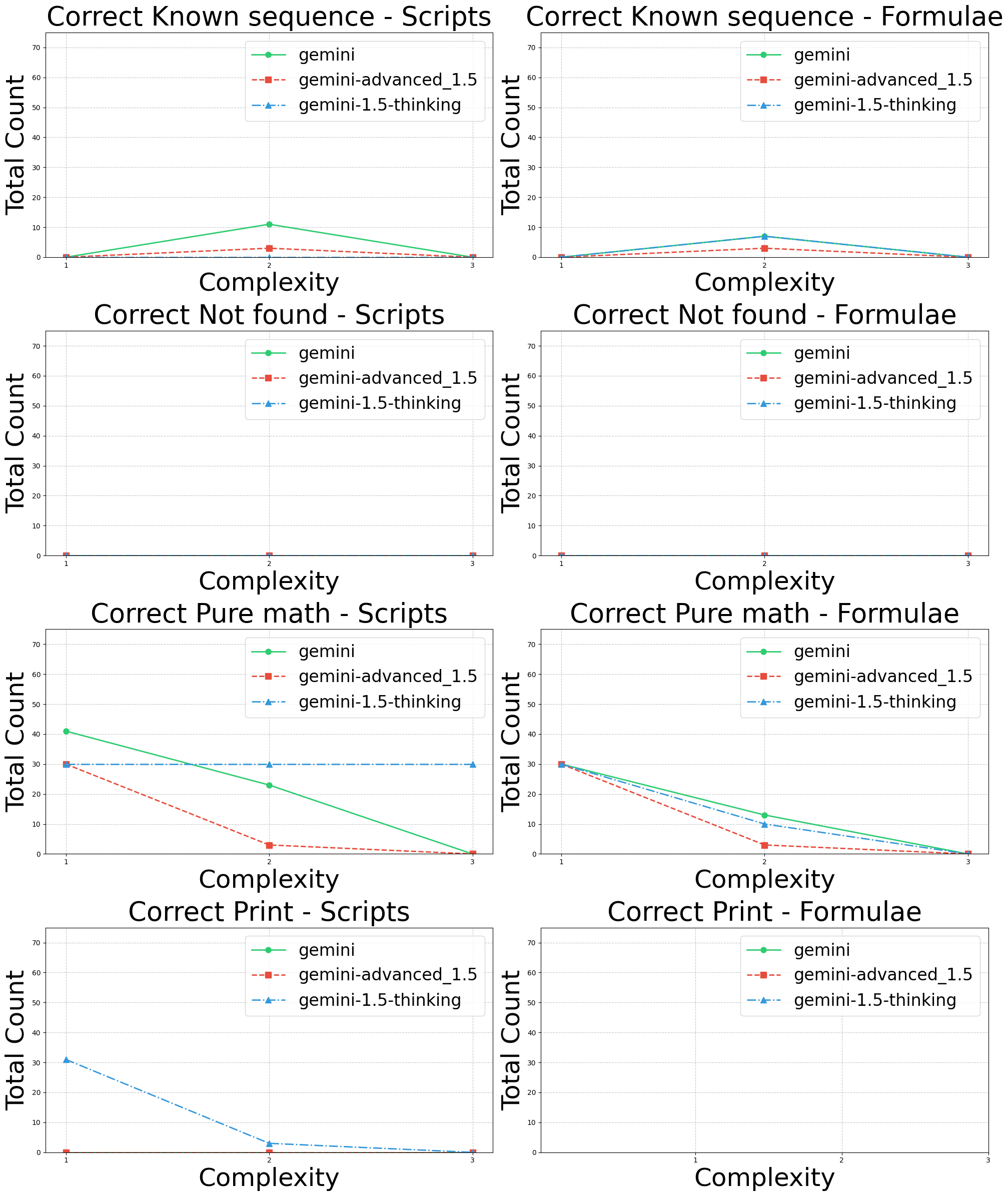
Figure 18: Comparison of the distribution of types of instances among the correct ones. Correct instances refer to Python scripts or formulae that correctly generate the target sequence. Known sequences refer to well-known numeric series such as Fibonacci and primes. Instances of mathematical formulae are defined using mathematical or programming terms only. Print cases (only for Python scripts) involve simple Print(sequence) statements to generate the target sequence. ”Not Found” cases occur when Gemini declares itself unable to generate any expression. These results further demonstrate the underperformance of the 1.5 Advanced version, even in Print, known sequences, and pure mathematical formula cases.

Despite these advancements, experimental comparisons between versions of ChatGPT, as well as Gemini revealed notable underperformance of the newer versions in specific dimensions. For ChatGPT, the comparative analysis is summarised in Figures 11, 13, 15, and 17. For Gemini, the corresponding results are illustrated in Figures 14, 12, 16, and 18.

Figure 11 evaluates equivalence and accuracy for ChatGPT, where equivalence is defined as instances in which multiple Python scripts or formulae produce identical outputs, and accuracy represents the generation of the target numeric sequence. While ChatGPT-o1 exhibited similar trends to ChatGPT-4o for Python script generation, its performance for formulae was notably inferior, achieving less than 75% accuracy even for the simplest cases, compared to ChatGPT-4o’s consistent 100% accuracy. Furthermore, ChatGPT-o1 completely failed in generating accurate cases involving simple print commands for the target sequences. Interestingly, ChatGPT-4.5 demonstrates performance quite similar to that of ChatGPT-4o in Python script generation; however, its performance is inferior in the generation of formulae.

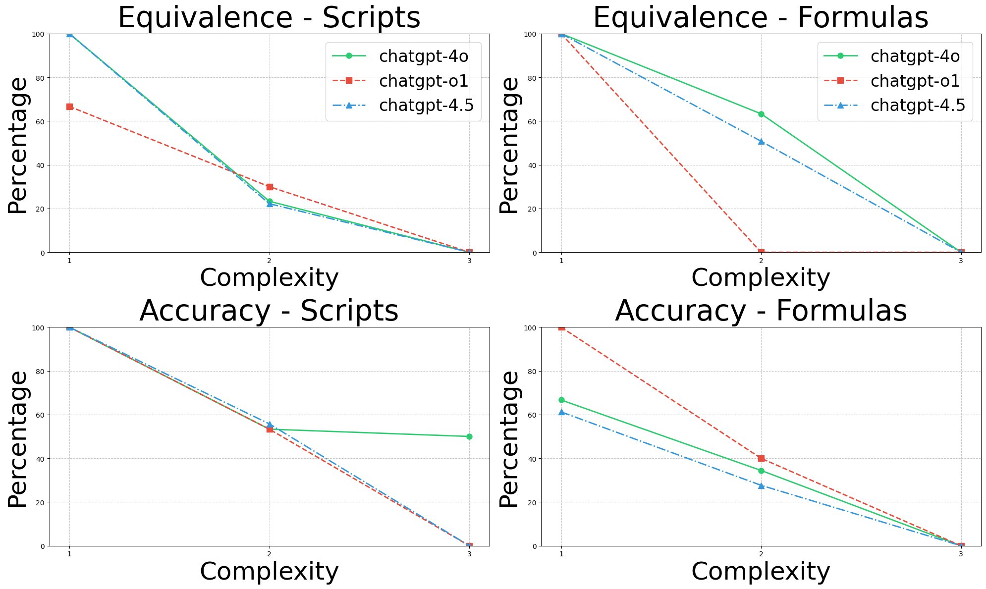
Figure 11: Comparison of equivalence and accuracy between ChatGPT-4o, ChatGPT-o1 and ChatGPT-4.5. Two or more scripts or formulae are deemed equivalent if they produce the same output, and accurate if they generate the target numeric sequence. The results show convergence inconsistencies or divergence with no clear goal or progress for newer versions under this test.

Gemini 1.5 Advanced Deep Research exhibited notable underperformance, particularly at higher levels of complexity. While demonstrating 100% accuracy and equivalence at lower complexity levels, its performance consistently declined or remained equal to Gemini 1.5 Thinking and Gemini Flash as complexity increased. This trend was further accentuated by the absence of print-based strategies (except in the 1.5 Thinking version) and a higher incidence of ”Not Found” cases during formula generation (as depicted in Figure 16).

While Gemini explicitly acknowledged its inability to generate solutions for certain sequences, thereby avoiding simplistic approaches like relying on print-based scripts or referencing known sequences, this combination of outcomes suggests a potential trade-off. While potentially reducing hallucinations, it may also indicate a degradation in creativity and problem-solving capacity.

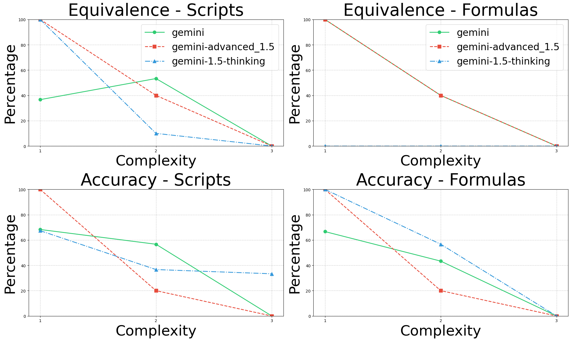
Figure 12: Comparison of equivalence and accuracy percentages between Gemini 1.5 Flash, Gemini 1.5 Advanced Deep Research and Gemini 1.5 Thinking. Equivalence measures the similarity of outputs between multiple Python scripts and multiple formulae generated for numeric sequences, while accuracy indicates the percentage of instances that correctly generate the target numeric sequence. A significant underperformance of the version 1.5 Advanced Deep Research is observed at higher complexity levels.

The disparity between the models is evident when considering the valid cases, as shown in Figures 13 for the ChatGPT case and in Figure 14 for Gemini. These figures illustrate the total number of valid instances, defined as scripts or formulae that can be executed or evaluated without errors. ChatGPT-o1 consistently produced fewer valid instances than ChatGPT-4o, often approaching zero in certain cases.

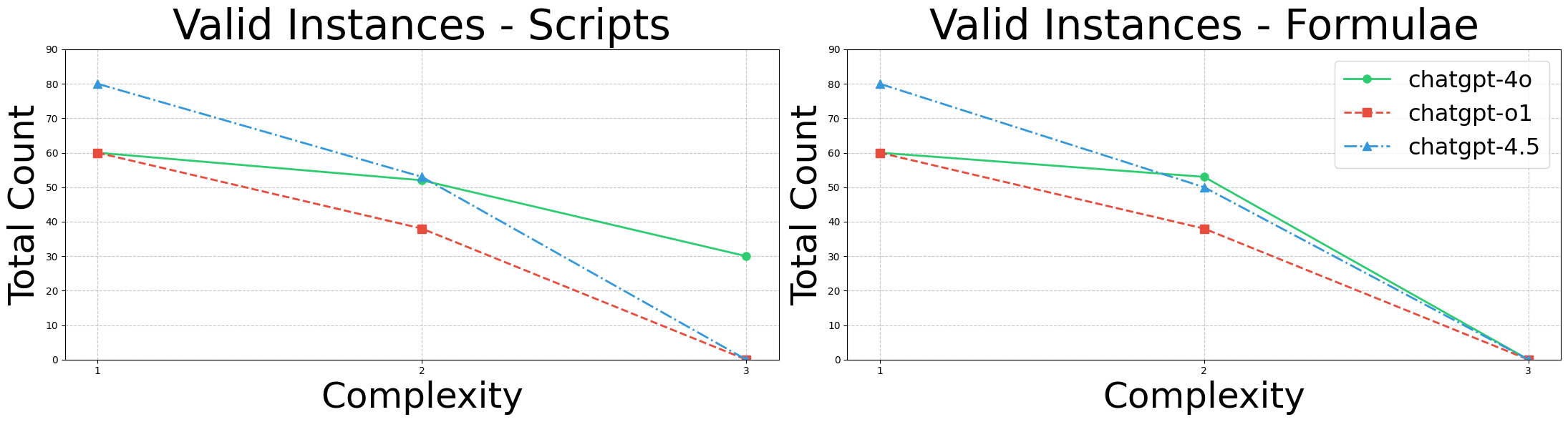
Figure 13: Comparison of the total number of valid instances between ChatGPT–4o, ChatGPT–o1 and ChatGPT–4.5. Valid instances are those that produce interpretable results without execution errors.

In the case of Gemini, the difference is even more pronounced, with a significant negative separation observed in cases of low complexity.

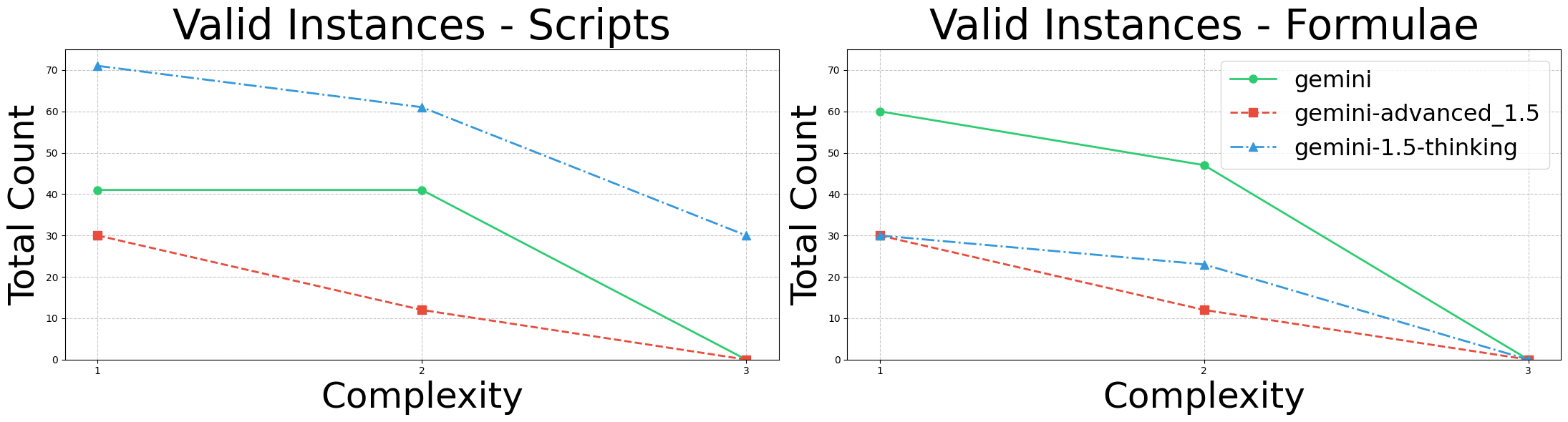
Figure 14: Comparison of valid instances between Gemini 1.5 Flash, Gemini 1.5 Deep Research and Gemini 1.5 Thinking. Valid instances refer to Python scripts and formulae that generate an output without execution errors.

A deeper insight is gained when considering the distribution of instance types among the total generated. For ChatGPT, these results are shown in Figure 15. ”Not Found” cases, where the model explicitly states its inability to generate an expression, were more prevalent in ChatGPT-o1. Furthermore, ChatGPT-o1 consistently underperformed in all other categories, including known sequences (e.g., primes, Fibonacci), mathematical formulae cases, and Python-specific cases, compared to ChatGPT-4o. This trend is further reinforced by the smaller number of total instances produced by ChatGPT-o1.

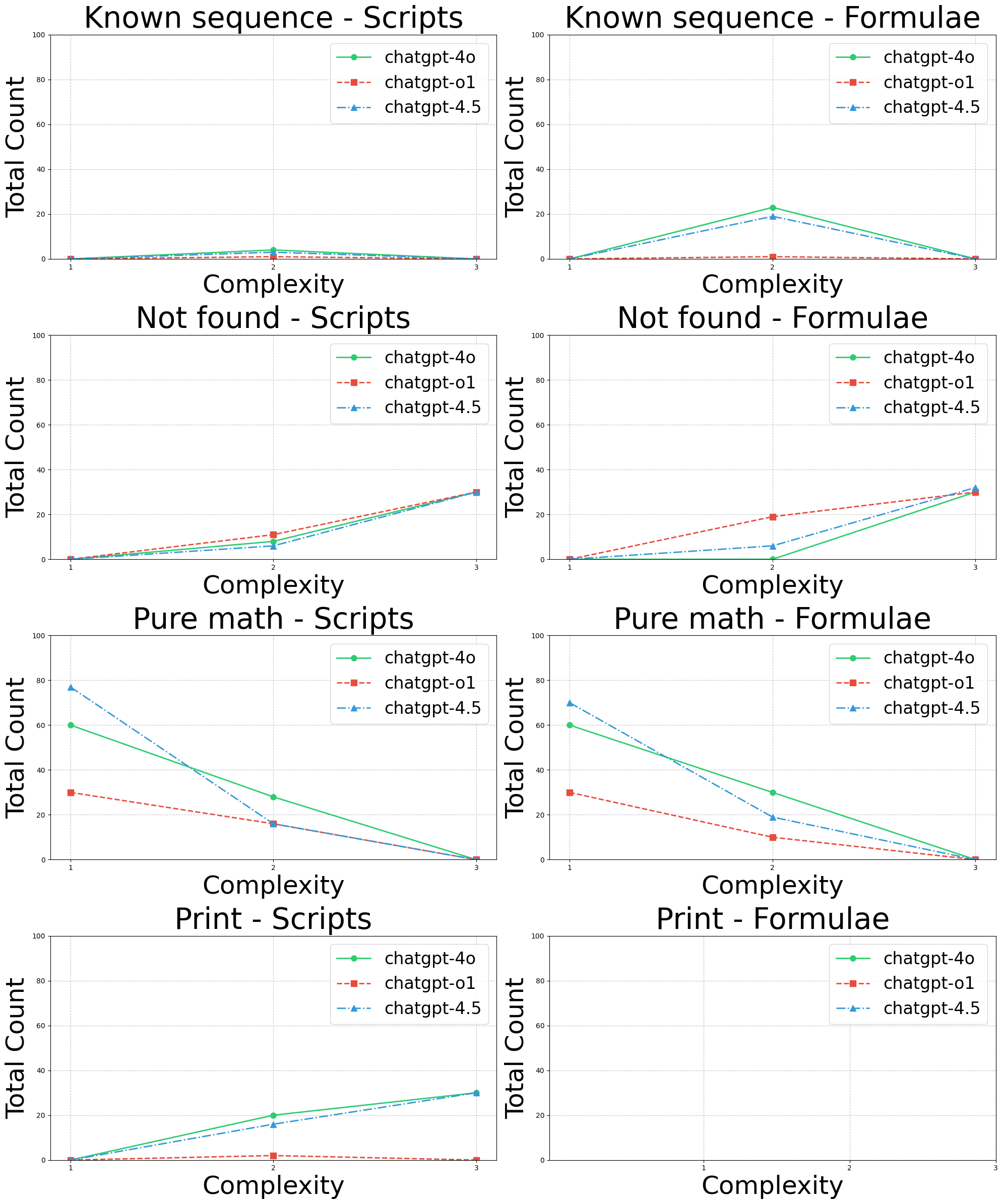
Figure 15: Comparison of the types of formulae and scripts produced by ChatGPT–4o, ChatGPT–o1 and ChatGPT–4.5. Known sequences refer to established numeric series such as Fibonacci, while ”Not Found” cases indicate the model’s explicit acknowledgement of failure.

The same trend is evident in the case of Gemini, as shown in Figure 16, where the version 1.5 Advanced Deep Research consistently performs poorly. This difference is particularly noticeable when considering the total number of instances generated, and is further reinforced by the fact that the newer version tends to generate more ”Not Found” cases.

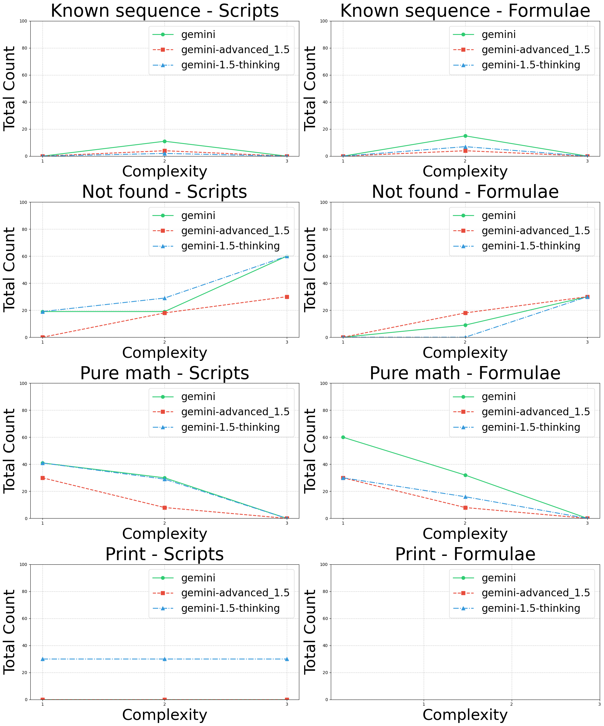
Figure 16: Comparison between Gemini 1.5 Flash, Gemini 1.5 Advanced Deep Research and Gemini 1.5 Thinking of the total count of instances by type among the total generated. Known sequences refer to well-known and documented numeric series such as Fibonacci and primes. Pure math instances are those defined in terms of mathematical formulae or programming terms only. Print cases (only for Python scripts) refer to instances where a simple Print(sequence) generates the target sequence. “Not Found” cases are those where Gemini declares its inability to generate an expression. These results show the underperformance of Gemini 1.5 Advanced in terms of total counts, with a notable absence of Print cases, which is the simplest and most effective way to generate a sequence.

Lastly, Figures 17 and 18 consolidate these findings by comparing the types of correct instances across both models. Both ChatGPT and Gemini consistently generated fewer correct outputs than their predecessor versions, further substantiating the observed performance gap.

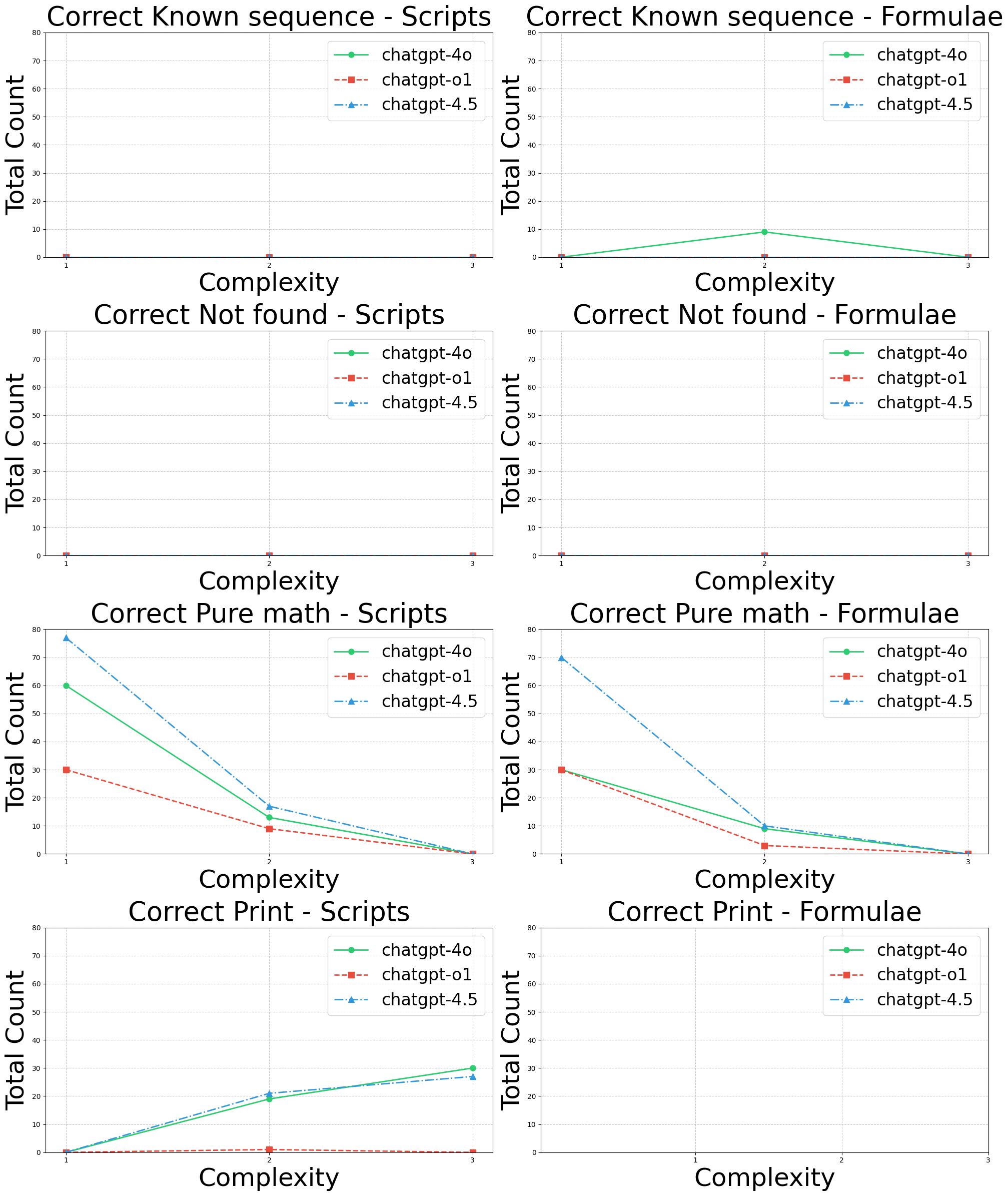
Figure 17: Comparison of correct instances between ChatGPT–4o, ChatGPT–o1 and ChatGPT–4.5. An instance is considered correct if it accurately generates the target sequence. ChatGPT–4.5 performed slightly better for simpler sequences.

Through this analysis, we can explain and justify the impact of the enhancements made to large language models (LLMs) in general. As mentioned at the beginning of this section, all changes can be attributed to technical improvements in processing speed, dataset quality, and hardware optimisation. However, the fundamental theory underpinning the transformer architecture remains unchanged. Although these improvements may make models more optimal for commercial use, they do not enhance or increase the level of general intelligence. In fact, they appear to move in the opposite direction, degrading not only the number of possible solutions in tasks that require intrinsic intelligence, such as improvisation, imagination, and analysis, but also the quality and accuracy of the outputs.

Sample of Sequences Testing Set

The following is a sample test for testing purposes used throughout the paper:

List of ‘climbers’

0, 0, 0, 0, 0, 0, 0
0, 0, 0, 0, 0, 0, 0
0, 0, 0, 0, 1, 0, 0
0, 0, 0, 0, 0, 1, 0, 0
0, 0, 0, 0, 0, 0, 1, 1
0, 0, 0, 0, 0, 0, 0, 1
0, 0, 0, 0, 0, 0, 0, 1
0, 0, 0, 1, 1, 0, 0, 0
0, 0, 1, 0, 0, 0, 0, 0
0, 1, 0, 1, 0, 1, 0, 1
0, 0, 0, 0, 1, 1, 1, 0
0, 0, 0, 0, 0, 0, 0, 1, 0
0, 0, 0, 0, 0, 0, 0, 0, 1
0, 0, 0, 0, 0, 0, 0, 0, 1
0, 0, 0, 0, 0, 1, 1, 0, 1
0, 1, 0, 1, 0, 1, 0, 1, 0
0, 0, 1, 0, 1, 0, 1, 0, 1
0, 1, 1, 0, 1, 1, 0, 1, 1
0, 0, 0, 0, 0, 0, 0, 0, 0
0, 0, 1, 0, 1, 0, 1, 1, 0
0, 1, 0, 1, 0, 0, 1, 0, 0
0, 1, 0, 1, 0, 1, 1, 0, 1
0, 0, 0, 1, 0, 1, 0, 1, 0, 1
0, 1, 0, 1, 0, 1, 0, 1, 0, 1

Binary Sequences

1, 1, 0, 0, 0, 1, 0, 0, 0, 0, 1 0, 0, 0, 1, 0, 1, 1, 0, 1, 0, 1 1, 0, 0, 0, 0, 1, 1, 1, 1, 0, 0 1, 1, 1, 1, 1, 1, 1, 1, 0, 1, 0 1, 0, 1, 1, 0, 1, 0, 1, 0, 1, 0 1, 1, 1, 0, 0, 1, 1, 0, 1, 1, 0 0, 0, 1, 1, 1, 0, 0, 1, 0, 1, 1 1, 1, 1, 0, 0, 0, 0, 0, 0, 0, 0 0, 1, 1, 1, 1, 0, 1, 0, 1, 1, 1 1, 1, 0, 0, 0, 1, 1, 1, 0, 1, 1 1, 0, 0, 1, 1, 0, 1, 0, 0, 0, 1 0, 1, 1, 1, 0, 1, 1, 0, 1, 1, 0 1, 0, 1, 0, 0, 1, 0, 1, 0, 1, 1 0, 1, 1, 0, 0, 1, 1, 1, 1, 0, 0 0, 0, 1, 1, 1, 1, 1, 0, 1, 1, 1 1, 1, 1, 0, 1, 1, 1, 0, 0, 1, 0 1, 0, 1, 0, 1, 0, 0, 0, 0, 0, 0 0, 0, 1, 1, 1, 1, 1, 1, 0, 1, 1 1, 1, 0, 0, 0, 1, 0, 1, 0, 1, 0 0, 0, 0, 0, 0, 1, 0, 1, 1, 0, 1 0, 0, 1, 1, 1, 1, 1, 1, 0, 0, 1 0, 1, 0, 0, 1, 0, 0, 1, 0, 1, 1 1, 0, 0, 1, 1, 0, 0, 0, 0, 0, 0 1, 1, 0, 1, 1, 1, 0, 0, 1, 1, 1 0, 0, 0, 0, 0, 0, 0, 1, 0, 0, 0 0, 1, 0, 0, 1, 1, 1, 1, 1, 1, 0 0, 0, 1, 0, 0, 0, 1, 0, 0, 0, 0 1, 0, 0, 0, 1, 1, 0, 0, 1, 1, 0 1, 1, 0, 0, 1, 0, 0, 0, 0, 0, 0 1, 0, 1, 0, 1, 0, 1, 0, 0, 1, 1 1, 0, 1, 1, 0, 1, 1, 1, 1, 1, 0 0, 0, 0, 0, 0, 0, 1, 0, 0, 0, 0 0, 1, 1, 0, 0, 0, 0, 0, 0, 0, 1 0, 0, 1, 1, 0, 1, 1, 0, 1, 1, 0 0, 0, 0, 0, 1, 1, 1, 1, 1, 0, 1 1, 1, 1, 0, 0, 0, 0, 1, 1, 1, 1 1, 0, 1, 0, 0, 1, 1, 1, 1, 1, 1 0, 1, 0, 0, 0, 0, 0, 0, 1, 0, 1 0, 1, 0, 0, 0, 1, 0, 1, 1, 1, 0 1, 0, 1, 0, 1, 1, 1, 0, 1, 0, 1 1, 0, 0, 0, 0, 1, 0, 0, 1, 1, 1 1, 1, 0, 0, 0, 0, 1, 0, 0, 0, 1 1, 0, 1, 0, 0, 0, 1, 0, 1, 0, 0 0, 0, 1, 1, 1, 1, 0, 0, 1, 0, 1 0, 0, 0, 0, 0, 0, 1, 0, 0, 0, 1 1, 1, 1, 1, 0, 0, 1, 1, 1, 0, 0 1, 0, 1, 0, 1, 1, 0, 1, 0, 1, 1 1, 0, 0, 1, 0, 1, 1, 1, 1, 1, 1 1, 1, 1, 1, 1, 0, 0, 0, 1, 1, 1 0, 0, 0, 1, 0, 1, 1, 1, 0, 0, 1 0, 0, 1, 0, 1, 0, 0, 1, 0, 0, 0 1, 1, 1, 0, 0, 1, 1, 1, 0, 1, 1 1, 0, 0, 1, 1, 1, 0, 1, 1, 1, 1 1, 0, 0, 1, 0, 0, 1, 1, 0, 0, 1 0, 0, 0, 0, 0, 0, 1, 1, 0, 1, 1 1, 0, 0, 1, 1, 0, 0, 1, 1, 1, 1 1, 1, 1, 1, 1, 0, 0, 1, 0, 0, 0 0, 1, 1, 1, 0, 1, 1, 1, 1, 1, 1 1, 0, 1, 0, 0, 1, 0, 0, 1, 1, 0 0, 1, 0, 0, 0, 1, 1, 0, 0, 1, 1 0, 0, 0, 0, 0, 1, 1, 0, 1, 1, 0 0, 1, 0, 0, 1, 0, 0, 1, 0, 0, 1 1, 1, 1, 0, 0, 1, 1, 1, 1, 1, 0 0, 1, 0, 1, 0, 1, 0, 0, 1, 1, 0 1, 1, 1, 0, 1, 0, 1, 0, 0, 0, 0 1, 0, 0, 0, 1, 0, 1, 1, 1, 1, 0 1, 0, 1, 0, 0, 0, 1, 0, 1, 1, 0 0, 0, 1, 0, 0, 1, 0, 1, 1, 0, 1 1, 0, 0, 1, 0, 1, 1, 0, 0, 1, 1 1, 1, 0, 0, 1, 1, 1, 0, 0, 1, 0 0, 0, 1, 0, 1, 1, 1, 0, 0, 1, 1 0, 1, 1, 1, 0, 1, 1, 0, 1, 1, 1 1, 0, 0, 0, 0, 1, 0, 0, 1, 0, 1 0, 1, 1, 1, 1, 0, 0, 1, 0, 0, 0 0, 0, 0, 0, 0, 1, 1, 1, 0, 1, 0 0, 1, 0, 1, 0, 1, 1, 0, 0, 1, 1 0, 0, 0, 1, 0, 0, 0, 0, 1, 0, 1 0, 1, 1, 0, 0, 0, 0, 0, 1, 1, 0 1, 0, 0, 1, 0, 1, 0, 1, 1, 0, 0 0, 1, 0, 1, 1, 1, 1, 1, 0, 1, 0 1, 0, 0, 1, 0, 0, 1, 0, 1, 1, 0 0, 1, 0, 1, 0, 1, 0, 1, 1, 1, 0 0, 0, 1, 0, 0, 1, 1, 0, 1, 0, 0 1, 1, 0, 0, 0, 0, 1, 1, 1, 1, 1 1, 0, 1, 1, 0, 0, 0, 1, 0, 0, 1 0, 1, 1, 1, 0, 0, 1, 1, 0, 0, 0 1, 0, 1, 1, 1, 0, 1, 0, 1, 0, 1 0, 1, 0, 1, 0, 0, 0, 0, 0, 0, 1 0, 1, 0, 0, 0, 1, 1, 0, 1, 0, 0 0, 0, 1, 0, 1, 0, 0, 0, 1, 1, 1 1, 0, 1, 1, 1, 0, 1, 1, 1, 0, 1 1, 1, 1, 1, 0, 1, 0, 1, 0, 0, 1 0, 0, 1, 1, 0, 0, 1, 0, 1, 0, 1 0, 1, 1, 0, 1, 0, 1, 0, 1, 1, 1 1, 0, 1, 0, 1, 0, 1, 1, 0, 0, 1 1, 0, 1, 1, 1, 1, 1, 0, 1, 1, 1 0, 1, 0, 1, 0, 0, 1, 1, 0, 1, 0 0, 0, 0, 1, 0, 1, 0, 0, 1, 1, 1 1, 1, 1, 0, 0, 0, 1, 1, 1, 1, 1 1, 0, 0, 0, 1, 1, 1, 0, 1, 1, 0

Example of Numerical Sequences

Complexity 1 Complexity 2 Complexity 3 2, 4, 6, 8, 10, 12, 14, 16, 18, 20 2, 3, 5, 7, 11, 13, 17, 19, 23, 29 29, 57, 68, 120, 134, 140, 173, 197, 283, 313 3, 6, 9, 12, 15, 18, 21, 24, 27, 30 1, 1, 2, 3, 5, 8, 13, 21, 34, 55 24, 26, 36, 40, 184, 226, 244, 384, 391, 423 4, 8, 12, 16, 20, 24, 28, 32, 36, 40 1, 2, 4, 8, 16, 32, 64, 128, 256, 512 90, 203, 212, 235, 270, 324, 342, 352, 371, 417 5, 10, 15, 20, 25, 30, 35, 40, 45, 50 1, 3, 9, 27, 81, 243, 729, 2187, 6561, 19683 20, 48, 95, 234, 282, 296, 352, 402, 428, 481 6, 12, 18, 24, 30, 36, 42, 48, 54, 60 1, 4, 9, 16, 25, 36, 49, 64, 81, 100 62, 98, 130, 154, 290, 315, 324, 385, 408, 447 7, 14, 21, 28, 35, 42, 49, 56, 63, 70 1, 8, 27, 64, 125, 216, 343, 512, 729, 1000 2, 42, 66, 102, 153, 195, 201, 252, 306, 396 8, 16, 24, 32, 40, 48, 56, 64, 72, 80 1, 1, 2, 6, 24, 120, 720, 5040, 40320, 362880 128, 151, 153, 217, 224, 332, 382, 400, 450, 478 9, 18, 27, 36, 45, 54, 63, 72, 81, 90 1, 3, 6, 10, 15, 21, 28, 36, 45, 55 26, 50, 114, 148, 160, 170, 274, 347, 432, 497 10, 20, 30, 40, 50, 60, 70, 80, 90, 100 2, 1, 3, 4, 7, 11, 18, 29, 47, 76 48, 94, 176, 177, 219, 276, 282, 283, 459, 488 1, 3, 5, 7, 9, 11, 13, 15, 17, 19 0, 1, 2, 5, 12, 29, 70, 169, 408, 985 139, 252, 272, 281, 304, 361, 370, 415, 438, 500 2, 4, 6, 8, 10, 12, 14, 16, 18, 20 1, 4, 27, 256, 3125, 46656, 823543, 16777216, 387420489, 10000000000 15, 95, 115, 195, 240, 318, 326, 350, 432, 450 11, 12, 13, 14, 15, 16, 17, 18, 19, 20 1, 2, 6, 20, 70, 252, 924, 3432, 12870, 48620 134, 224, 293, 378, 379, 395, 434, 451, 482, 496 21, 22, 23, 24, 25, 26, 27, 28, 29, 30 2, 3, 5, 7, 11, 13, 17, 19, 23, 29 23, 93, 142, 145, 245, 266, 296, 317, 428, 495 31, 32, 33, 34, 35, 36, 37, 38, 39, 40 4, 6, 9, 10, 14, 15, 21, 22, 25, 26 18, 39, 71, 194, 197, 219, 263, 270, 416, 473 41, 42, 43, 44, 45, 46, 47, 48, 49, 50 1, 10, 11, 100, 101, 110, 111, 1000, 1001, 1010 9, 84, 144, 170, 325, 393, 401, 405, 435, 497 51, 52, 53, 54, 55, 56, 57, 58, 59, 60 0, 1, 81, 512, 2401, 4913, 5832, 17576, 19683, 234256 26, 40, 202, 267, 282, 340, 359, 408, 410, 495 61, 62, 63, 64, 65, 66, 67, 68, 69, 70 1, 2, 145, 40585 34, 92, 164, 165, 209, 296, 414, 456, 467, 494 71, 72, 73, 74, 75, 76, 77, 78, 79, 80 2, 5, 12, 20, 29, 39, 50, 62, 75, 89 16, 119, 121, 123, 135, 139, 285, 311, 409, 412 81, 82, 83, 84, 85, 86, 87, 88, 89, 90 1, 8, 10, 18, 19, 100, 101, 108, 109, 110 8, 11, 12, 103, 116, 196, 247, 254, 389, 427 91, 92, 93, 94, 95, 96, 97, 98, 99, 100 3, 7, 31, 127, 2047, 8191, 131071, 524287, 8388607, 536870911 12, 36, 96, 119, 171, 213, 221, 232, 363, 451 101, 102, 103, 104, 105, 106, 107, 108, 109, 110 1, 2, 4, 8, 16, 23, 28, 38, 58, 89 38, 91, 142, 197, 215, 313, 316, 319, 423, 466 111, 112, 113, 114, 115, 116, 117, 118, 119, 120 1, 2, 4, 8, 15, 26, 42, 64, 93, 129 7, 42, 147, 201, 213, 248, 310, 332, 436, 479 121, 122, 123, 124, 125, 126, 127, 128, 129, 130 1, 5, 12, 22, 35, 51, 70, 92, 117, 145 27, 101, 105, 164, 245, 290, 304, 441, 449, 490 131, 132, 133, 134, 135, 136, 137, 138, 139, 140 0, 1, 1, 2, 1, 2, 2, 3, 1, 3 4, 11, 29, 106, 214, 283, 296, 298, 360, 497 141, 142, 143, 144, 145, 146, 147, 148, 149, 150 1, 2, 5, 15, 52, 203, 877, 4140, 21147, 115975 72, 106, 139, 165, 171, 192, 199, 429, 453, 477 151, 152, 153, 154, 155, 156, 157, 158, 159, 160 2, 3, 5, 7, 11, 13, 17, 19, 23, 29 187, 218, 260, 295, 301, 314, 379, 410, 452, 469 161, 162, 163, 164, 165, 166, 167, 168, 169, 170 1, 11, 21, 1211, 111221 29, 63, 95, 140, 150, 190, 221, 437, 482, 491 171, 172, 173, 174, 175, 176, 177, 178, 179, 180 2, 3, 5, 7, 11, 13, 17, 19, 23, 29 3, 11, 84, 144, 156, 177, 188, 199, 229, 284 181, 182, 183, 184, 185, 186, 187, 188, 189, 190 1, 2, 4, 8, 16, 32, 64, 128, 256, 512 26, 94, 98, 137, 176, 301, 323, 330, 372, 444 191, 192, 193, 194, 195, 196, 197, 198, 199, 200 1, 3, 7, 15, 31, 63, 127, 255, 511, 1023 39, 81, 88, 210, 215, 378, 416, 430, 439, 490

References

- [1] C. Spearman, “"general intelligence," objectively determined and measured,” The American Journal of Psychology, vol. 15, no. 2, pp. 201–292, 1904.
- [2] N. Gauvrit, H. Zenil, F. Soler-Toscano, J.-P. Delahaye, and P. Brugger, “Human behavioral complexity peaks at age 25,” PLoS Computational Biology, vol. 13, no. 4, p. e1005408, 2017.
- [3] H. Zenil, J. A. R. Marshall, and J. Tegnér, “Approximations of algorithmic and structural complexity validate cognitive-behavioural experimental results,” Frontiers in Computational Neuroscience, vol. 16, 2023.
- [4] H. Zenil, “On the complex behaviour of natural and artificial machines and systems,” in Metrics of Sensory Motor Integration in Robots and Animals, ser. Cognitive Systems Monographs, F. P. Bonsignorio, A. P. del Pobil, E. Messina, and J. Hallam, Eds. Springer, 2019, pp. 111–125.
- [5] ——, “Compression is comprehension, and the unreasonable effectiveness of digital computation in the natural world,” in Unravelling Complexity: The Life and Work of Gregory Chaitin, S. Wuppuluri and F. Doria, Eds. World Scientific Publishing, 2019, pp. 173–208.
- [6] J. Hernández-Orallo and N. Minaya-Collado, “A formal definition of intelligence based on an intensional variant of algorithmic complexity,” in International Symposium of Engineering of Intelligent Systems (EIS98), 1998, pp. 146–163.
- [7] A. M. Turing, “Computing machinery and intelligence,” Mind, vol. LIX, no. 236, pp. 433–460, 1950.
- [8] D. Hofstadter, Gödel, Escher, Bach: An Eternal Golden Braid, ser. Harvester studies in cognitive science. Penguin, 2000.
- [9] G. J. Chaitin, “Gödel’s theorem and information,” International Journal of Theoretical Physics, vol. 21, no. 12, pp. 941–954, Dec. 1982. [Online]. Available: http://dx.doi.org/10.1007/BF02084159
- [10] R. Solomonoff, The Application of Algorithmic Probability to Problems in Artificial Intelligence. Elsevier, 1986, pp. 473–491. [Online]. Available: http://dx.doi.org/10.1016/B978-0-444-70058-2.50040-1
- [11] M. Hutter, Universal Artificial Intelligence: Sequential Decisions Based on Algorithmic Probability, ser. Texts in Theoretical Computer Science. An EATCS Series. Springer, Berlin, Heidelberg, 2005.
- [12] S. Legg and M. Hutter, Tests of Machine Intelligence. Springer Berlin Heidelberg, 2007, pp. 232–242. [Online]. Available: http://dx.doi.org/10.1007/978-3-540-77296-5_22
- [13] H. Zenil, “A turing test-inspired approach to natural computation,” in Turing in Context II, Historical and Contemporary Research in Logic, Computing Machinery and Artificial Intelligence, G. Primiero and L. De Mol, Eds. Belgium: Royal Flemish Academy of Belgium for Science and the Arts, 2013.
- [14] J. Hernández-Orallo, C-Tests Revisited: Back and Forth with Complexity. Springer International Publishing, 2015, pp. 272–282. [Online]. Available: http://dx.doi.org/10.1007/978-3-319-21365-1_28
- [15] P. Belcak, F. Schenker, A. Kastrati, and R. Wattenhofer, “Fact: learning governing abstractions behind integer sequences,” in Proceedings of the 36th International Conference on Neural Information Processing Systems, ser. NIPS ’22. Red Hook, NY, USA: Curran Associates Inc., 2022.
- [16] I. Sutskever, “Talk at the Simons Institute: Ilya Sutskever (OpenAI),” Video; Simons Institute for the Theory of Computing, August 14 2023. [Online]. Available: https://simons.berkeley.edu/talks/ilya-sutskever-openai-2023-08-14
- [17] AI News, “AI compresses reality to small vector space: Elon Musk,” Online, 2021, last updated December 28, 2021. [Online]. Available: https://analyticsindiamag.com/ai-news-updates/ai-compresses-reality-to-small-vector-space-elon-musk/
- [18] S. Hernández-Orozco, H. Zenil, J. Riedel, A. Uccello, N. A. Kiani, and J. Tegnér, “Algorithmic probability-guided machine learning on non-differentiable spaces,” Frontiers in Artificial Intelligence, vol. 4, p. 25, 2021. [Online]. Available: https://doi.org/10.3389/frai.2021.658282
- [19] H. Zenil, N. Kiani, F. Marabita, Y. Deng, S. Elias, A. Schmidt, G. Ball, and J. Tegnér, “An Algorithmic Information Calculus for Causal Discovery and Reprogramming Systems,” iScience, 2019, s2589-0042(19)30270-6.
- [20] H. Zenil, N. Kiani, A. Zea, and J. Tegnér, “Causal Deconvolution by Algorithmic Generative Models,” Nature Machine Intelligence, vol. 1, pp. 58–66, 2019.
- [21] A. N. Kolmogorov, “Three approaches to the quantitative definition of information,” Problems of Information Transmission, vol. 1, no. 1, pp. 1–7, 1965.
- [22] G. J. Chaitin, “On the length of programs for computing finite binary sequences,” Journal of the ACM (JACM), vol. 13, no. 4, pp. 547–569, 1966.
- [23] R. Solomonoff, “A Formal Theory of Inductive Inference,” Information and Control, vol. 7, no. 1, pp. 1–22, 1964.
- [24] C. S. Calude, Information and Randomness: An algorithmic perspective, 2nd ed. Springer-Verlag, 2002.
- [25] R. G. Downey and D. R. Hirschfeldt, Algorithmic Randomness and Complexity, ser. Theory and Applications of Computability. New York, NY: Springer New York, 2010. [Online]. Available: http://link.springer.com/10.1007/978-0-387-68441-3
- [26] M. Li and P. Vitányi, An Introduction to Kolmogorov Complexity and Its Applications, 4th ed. Springer, 2019.
- [27] F. Chollet, “On the measure of intelligence,” arXiv preprint arXiv:1911.01547, 2019. [Online]. Available: https://arxiv.org/abs/1911.01547
- [28] Y. LeCun, “A path towards autonomous machine intelligence,” OpenReview Archive, June 27 2022. [Online]. Available: https://openreview.net/forum?id=BZ5a1r-kVsf
- [29] M. Assran, Q. Duval, I. Misra, P. Bojanowski, P. Vincent, M. Rabbat, Y. LeCun, and N. Ballas, “Self-supervised learning from images with a joint-embedding predictive architecture,” arXiv preprint arXiv:2301.08243 [cs.CV], 2023.
- [30] H. Zenil, “Compression is comprehension and the unreasonable effectiveness of digital computation in the natural world,” in UNRAVELLING COMPLEXITY: The Life and Work of Gregory Chaitin. World Scientific, 2020, pp. 201–238.
- [31] L. Levin, “Universal Search Problems and Algorithmic Probability,” Problems of Information Transmission, vol. 9, no. 3, pp. 265–266, 1973.
- [32] W. Kirchherr, M. Li, and P. Vitányi, “The miraculous universal distribution,” The Mathematical Intelligencer, vol. 19, pp. 7–15, 1997.
- [33] H. Zenil, F. Soler-Toscano, and J. J. Joosten, “Empirical Encounters with Computational Irreducibility and Unpredictability,” Minds and Machines, vol. 22, no. 3, pp. 149–165, 2012.
- [34] H. Zenil, “A Review of Methods for Estimating Algorithmic Complexity: Options, Challenges, and New Directions,” Entropy, vol. 22, no. 612, 2020.
- [35] A. Agrawal, J. Gans, and A. Goldfarb, Prediction Machines: The Simple Economics of Artificial Intelligence. Boston, MA: Harvard Business Review Press, 2018.
- [36] ——, Power and Prediction: The Disruptive Economics of Artificial Intelligence. Boston, MA: Harvard Business Review Press, 2022.
- [37] L. A. Levin, “Various measures of complexity for finite objects (axiomatic description),” Soviet Math. Doklady, vol. 17, no. 2, pp. 522–526, 1976.
- [38] ——, “Laws of information conservation (nongrowth) and aspects of the foundation of probability theory,” Problems of Information Transmission, vol. 10, no. 3, pp. 206–210, 1974.
- [39] ——, “On the notion of a random sequence,” Soviet Math. Doklady, vol. 14, no. 5, pp. 1413–1416, 1973.
- [40] R. von Mises, Wahrscheinlichkeit, Statistik und Wahrheit. Vienna: Springer-Verlag, 1928.
- [41] C.-P. Schnorr, Zufälligkeit und Wahrscheinlichkeit. Eine Algorithmische Begründung der Wahrscheinlichkeitstheorie. Springer, 1971.
- [42] ——, “A unified approach to the definition of random sequences,” Mathematical Systems Theory, vol. 5, no. 3, pp. 246–258, 1971.
- [43] J. Schmidhuber, “Gödel Machines: Fully Self-referential Optimal Universal Self-improvers,” in Artificial General Intelligence, ser. Cognitive Technologies, B. Goertzel and C. Pennachin, Eds. Springer, Berlin, Heidelberg, 2007, pp. 199–226.
- [44] E. Glazer, E. Erdil, T. Besiroglu, D. Chicharro, E. Chen, A. Gunning, C. F. Olsson, J.-S. Denain, A. Ho, E. de Oliveira Santos, O. JÀrviniemi, M. Barnett, R. Sandler, M. Vrzala, J. Sevilla, Q. Ren, E. Pratt, L. Levine, G. Barkley, N. Stewart, B. Grechuk, T. Grechuk, S. V. Enugandla, and M. Wildon, “Frontiermath: A benchmark for evaluating advanced mathematical reasoning in ai,” arXiv preprint arXiv:2411.04872, 2024. [Online]. Available: https://arxiv.org/abs/2411.04872
- [45] K. F. Hubert, K. N. Awa, and D. L. Zabelina, “The current state of artificial intelligence generative language models is more creative than humans on divergent thinking tasks,” Scientific Reports, vol. 14, no. 1, p. 3440, 2024.
- [46] I. Mirzadeh, K. Alizadeh, H. Shahrokhi, O. Tuzel, S. Bengio, and M. Farajtabar, “Gsm-symbolic: Understanding the limitations of mathematical reasoning in large language models,” arXiv preprint arXiv:2410.05229, 2024. [Online]. Available: https://arxiv.org/abs/2410.05229
- [47] D. Schuurmans, H. Dai, and F. Zanini, “Autoregressive Large Language Models are Computationally Universal,” arXiv preprint arXiv:2410.03170, 2024.
- [48] M. Aljanabi, M. Ghazi, A. H. Ali, S. A. Abed et al., “ChatGpt: open possibilities,” Iraqi Journal For Computer Science and Mathematics, vol. 4, no. 1, pp. 62–64, 2023.
- [49] L. Yizhen, H. Shaohan, Q. Jiaxing, Q. Lei, H. Dongran, and L. Zhongzhi, “Exploring the Comprehension of ChatGPT in Traditional Chinese Medicine Knowledge,” arXiv preprint arXiv:2403.09164, 2024.
- [50] D. Bayani, “Testing the Depth of ChatGPT’s Comprehension via Cross-Modal Tasks Based on ASCII-Art: GPT3. 5’s Abilities in Regard to Recognizing and Generating ASCII-Art Are Not Totally Lacking,” arXiv preprint arXiv:2307.16806, 2023.
- [51] F. Wei, X. Chen, and L. Luo, “Rethinking generative large language model evaluation for semantic comprehension,” arXiv preprint arXiv:2403.07872, 2024.
- [52] T. Zhong, Z. Liu, Y. Pan, Y. Zhang, Y. Zhou, S. Liang, Z. Wu, Y. Lyu, P. Shu, X. Yu et al., “Evaluation of OpenAI o1: Opportunities and Challenges of AGI,” arXiv preprint arXiv:2409.18486, 2024.
- [53] C. Si, D. Yang, and T. Hashimoto, “Can LLMS generate novel research ideas? a large-scale human study with 100+ NLP researchers,” arXiv preprint arXiv:2409.04109, 2024.
- [54] G. Marcus, “Deep learning is hitting a wall,” Nautilus, March 10 2022. [Online]. Available: https://nautil.us/deep-learning-is-hitting-a-wall-238440/
- [55] L. Feng, L. Zhang, and C. H. Lai, “Optimal machine intelligence at the edge of chaos,” arXiv preprint arXiv:1909.05176, 2019.
- [56] G. Marcus, The Algebraic Mind: Integrating Connectionism and Cognitive Science. Cambridge, MA: MIT Press, 2001.
- [57] J. M. Bishop, “Artificial intelligence is stupid and causal reasoning will not fix it,” Frontiers in Psychology, vol. 11, p. 513474, 2021.
- [58] H. Zenil, F. Soler Toscano, and N. Gauvrit, Methods and Applications of Algorithmic Complexity: Beyond Statistical Lossless Compression. Springer, 2022.
- [59] H. Zenil, N. A. Kiani, and J. Tegnér, Algorithmic Information Dynamics: A Computational Approach to Causality with Applications to Living Systems. Cambridge University Press, 2023.
- [60] L. A. Levin, “Randomness conservation inequalities: Information and independence in mathematical theories,” Information and Control, vol. 61, pp. 15–37, 1984.
- [61] H. Zenil, Ed., A Computable Universe: Understanding Computation and Exploring Nature as Computation. Singapore: World Scientific, 2012.
- [62] J.-P. Delahaye and H. Zenil, “Numerical evaluation of algorithmic complexity of short strings: A glance into the innermost structure of algorithmic randomness,” Applied Mathematics and Computation, vol. 219, pp. 63–77, 2012.
- [63] F. Soler-Toscano, H. Zenil, J.-P. Delahaye, and N. Gauvrit, “Calculating kolmogorov complexity from the output frequency distributions of small turing machines,” PLoS ONE, vol. 9, no. 5, p. e96223, 2014.
- [64] H. Zenil, F. Soler-Toscano, J.-P. Delahaye, and N. Gauvrit, “Two-dimensional kolmogorov complexity and validation of the coding theorem method by compressibility,” PeerJ Computer Science, vol. 1, p. e23, 2015.
- [65] J. Rissanen, “Modeling by shortest data description,” Automatica, vol. 14, no. 5, pp. 465–471, 1978.
- [66] H. Zenil and P. Minary, “Training-free measures based on algorithmic probability identify high nucleosome occupancy in dna sequences,” Nucleic Acids Research, vol. 47, no. 20, p. gkz750, 2019.
- [67] H. Zenil, J.-P. Delahaye, and C. Gaucherel, “Image characterization and classification by physical complexity,” Complexity, vol. 17, no. 3, pp. 26–42, 2012.
- [68] F. Soler-Toscano, H. Zenil, J.-P. Delahaye, and N. Gauvrit, “Correspondence and independence of numerical evaluations of algorithmic information measures,” Computability, vol. 2, no. 2, pp. 125–140, 2013.
- [69] H. Zenil, S. Hernández-Orozco, N. Kiani, F. Soler-Toscano, and A. Rueda-Toicen, “A Decomposition Method for Global Evaluation of Shannon Entropy and Local Estimations of Algorithmic Complexity,” Entropy, vol. 20, no. 8, p. 605, 2018.
- [70] H. Zenil, S. Hernández-Orozco, N. A. Kiani, F. Soler-Toscano, A. Rueda-Toicen, and J. Tegnér, “A decomposition method for global evaluation of Shannon entropy and local estimations of algorithmic complexity,” Entropy, vol. 20, no. 8, p. 605, 2018.
- [71] H. Zenil, N. Kiani, F. Abrahão, and J. Tegner, “Algorithmic information dynamics,” Scholarpedia, 2020.
- [72] C.-Y. Wang, A. DaghighFarsoodeh, and H. V. Pham, “Selection of prompt engineering techniques for code generation through predicting code complexity,” 2024. [Online]. Available: https://arxiv.org/abs/2409.16416
- [73] J. Li, G. Li, Y. Li, and Z. Jin, “Structured chain-of-thought prompting for code generation,” ACM Trans. Softw. Eng. Methodol., vol. 34, no. 2, Jan. 2025. [Online]. Available: https://doi.org/10.1145/3690635
- [74] F. Soler-Toscano, H. Zenil, J.-P. Delahaye, and N. Gauvrit, “Calculating kolmogorov complexity from the output frequency distributions of small turing machines,” PloS one, vol. 9, no. 5, p. e96223, 2014.
- [75] M. Tan, M. A. Merrill, V. Gupta, T. Althoff, and T. Hartvigsen, “Are language models actually useful for time series forecasting?” in The Thirty-eighth Annual Conference on Neural Information Processing Systems, 2024.
- [76] Y. Zhao, R. Zhang, W. Li, D. Huang, J. Guo, S. Peng, Y. Hao, Y. Wen, X. Hu, Z. Du et al., “Assessing and understanding creativity in large language models,” arXiv preprint arXiv:2401.12491, 2024.
- [77] M. Hutter, D. Quarel, and E. Catt, An Introduction to Universal Artificial Intelligence. Boca Raton, FL: CRC Press, May 2024.
- [78] H. Zenil, “A turing test-inspired approach to natural computation,” in Turing in Context II, Historical and Contemporary Research in Logic, Computing Machinery and Artificial Intelligence, G. Primiero and L. De Mol, Eds. Belgium: Royal Flemish Academy of Belgium for Science and the Arts, 2013.
- [79] S. Hernández-Orozco, N. Kiani, and H. Zenil, “Algorithmically Probable Mutations Reproduce Aspects of Evolution, such as Convergence Rate, Genetic Memory, and Modularity,” Royal Society Open Science, vol. 5, p. 180399, 2018.
- [80] F. Soler-Toscano and H. Zenil, “A Computable Measure of Algorithmic Probability by Finite Approximations with an Application to Integer Sequences,” Complexity, vol. 2017, p. Article ID 7208428, 2017.
- [81] F. Soler-Toscano, H. Zenil, J.-P. Delahaye, and N. Gauvrit, “Correspondence and Independence of Numerical Evaluations of Algorithmic Information Measures,” Computability, vol. 2, no. 2, pp. 125–140, 2013.
- [82] H. Zenil, N. A. Kiani, and J. Tegnér, “Low algorithmic complexity entropy-deceiving graphs,” Physical Review E, vol. 96, no. 1, p. 012308, 2017.
- [83] F. S. Abrahão, S. Hernández-Orozco, N. A. Kiani, J. Tegnér, and H. Zenil, “Assembly theory is an approximation to algorithmic complexity based on lz compression that does not explain selection or evolution,” PLOS Complex Systems, vol. 1, no. 1, p. e0000014, 2024.
- [84] B. S. Bloom, M. D. Engelhart, E. J. Furst, W. H. Hill, and D. R. Krathwohl, Taxonomy of Educational Objectives: The Classification of Educational Goals. Handbook 1: Cognitive Domain. New York: Longman, 1956.
- [85] J. Hernández-Orallo and D. L. Dowe, “Measuring universal intelligence: Towards an anytime intelligence test,” Artificial Intelligence, vol. 174, no. 18, pp. 1508–1539, Dec. 2010. [Online]. Available: http://dx.doi.org/10.1016/j.artint.2010.09.006
- [86] J. Hernández-Orallo, F. Martínez-Plumed, U. Schmid, M. Siebers, and D. L. Dowe, “Computer models solving intelligence test problems: Progress and implications,” Artificial Intelligence, vol. 230, pp. 74–107, Jan. 2016. [Online]. Available: http://dx.doi.org/10.1016/j.artint.2015.09.011
- [87] V. Corsino, J. M. Gilpérez, and L. Herrera, “Kitbit: A new ai model for solving intelligence tests and numerical series,” IEEE Transactions on Pattern Analysis and Machine Intelligence, vol. 45, no. 11, pp. 13 893–13 903, 2023.
- [88] A. S. et al., “Beyond the imitation game: Quantifying and extrapolating the capabilities of language models,” Transactions on Machine Learning Research, 2023. [Online]. Available: https://openreview.net/forum?id=uyTL5Bvosj
- [89] K. Zhu, J. Chen, J. Wang, N. Z. Gong, D. Yang, and X. Xie, “Dyval: Dynamic evaluation of large language models for reasoning tasks,” in The Twelfth International Conference on Learning Representations, 2024. [Online]. Available: https://openreview.net/forum?id=gjfOL9z5Xr
- [90] O. Yoran, K. Zheng, F. Gloeckle, J. Gehring, G. Synnaeve, and T. Cohen, “The koLMogorov test: Compression by code generation,” in The Thirteenth International Conference on Learning Representations, 2025. [Online]. Available: https://openreview.net/forum?id=C45YqeBDUM
- [91] J. Burden, M. Cebrian, and J. Hernandez-Orallo, “Conversational complexity for assessing risk in large language models,” 2024. [Online]. Available: https://arxiv.org/abs/2409.01247
- [92] S. I. Mirzadeh, K. Alizadeh, H. Shahrokhi, O. Tuzel, S. Bengio, and M. Farajtabar, “GSM-symbolic: Understanding the limitations of mathematical reasoning in large language models,” in The Thirteenth International Conference on Learning Representations, 2025. [Online]. Available: https://openreview.net/forum?id=AjXkRZIvjB
- [93] H. Wu, T. Hu, Y. Liu, H. Zhou, J. Wang, and M. Long, “TimesNet: Temporal 2D-Variation Modeling for General Time Series Analysis,” in International Conference on Learning Representations, 2023.
- [94] Y. Liu, T. Hu, H. Zhang, H. Wu, S. Wang, L. Ma, and M. Long, “itransformer: Inverted transformers are effective for time series forecasting,” arXiv preprint arXiv:2310.06625, 2023.
- [95] W. Shiyu, W. Haixu, S. Xiaoming, H. Tengge, L. Huakun, M. Lintao, Z. J. Y, and Z. Jun, “Timemixer: Decomposable multiscale mixing for time series forecasting,” arXiv preprint arXiv:2405.14616, 2024.
- [96] H. Wu, T. Hu, Y. Liu, H. Zhou, J. Wang, and M. Long, “Timesnet: Temporal 2d-variation modeling for general time series analysis,” in The eleventh international conference on learning representations, 2022.
- [97] Y. Jiang, Z. Pan, X. Zhang, S. Garg, A. Schneider, Y. Nevmyvaka, and D. Song, “Empowering Time Series Analysis with Large Language Models: A Survey,” 2024.
- [98] Ansari, A. Fatir, Stella, Lorenzo, Turkmen, Caner, Zhang, Xiyuan, Mercado, Pedro, Shen, Huibin, Shchur, Oleksandr, Rangapuram, S. Syndar, P. Arango, Sebastian, Kapoor, Shubham, Zschiegner, Jasper, Maddix, D. C., Mahoney, M. W., Torkkola, Kari, G. Wilson, Andrew, Bohlke-Schneider, Michael, Wang, and Yuyang, “Chronos: Learning the Language of Time Series,” arXiv preprint arXiv:2403.07815, 2024.
- [99] A. Garza and M. Mergenthaler-Canseco, “Timegpt-1,” 2023.
- [100] K. Rasul, A. Ashok, A. R. Williams, H. Ghonia, R. Bhagwatkar, A. Khorasani, M. J. D. Bayazi, G. Adamopoulos, R. Riachi, N. Hassen, M. Biloš, S. Garg, A. Schneider, N. Chapados, A. Drouin, V. Zantedeschi, Y. Nevmyvaka, and I. Rish, “Lag-Llama: Towards Foundation Models for Probabilistic Time Series Forecasting,” 2024.
- [101] A. V. Team, “GPT-4o vs OpenAI o1: A Comprehensive Comparison,” Blog; Analytics Vidhya, September 2024. [Online]. Available: https://www.analyticsvidhya.com/blog/2024/09/gpt-4o-vs-openai-o1/
- [102] C. Días, “Los cambios esenciales que llegan con gemini 2.0 y que le hacen mejor que chatgpt,” 2024, accessed: 2024-12-18. [Online]. Available: https://cincodias.elpais.com/smartlife/lifestyle/2024-12-18/gemini-20-cambios-mas-importantes.html?utm_source=chatgpt.com
- [103] G. Team, “Google Gemini: Next Generation Model,” Blog; Google Blog, February 2024, accessed: 2024-12-23. [Online]. Available: https://blog.google/technology/ai/google-gemini-next-generation-model-february-2024/#:˜:text=1.5%20Pro%20can%20perform%20highly,across%20longer%20blocks%20of%20code