Efficient automated cut-point finder in high-dimensional Cox models: a simple but promising approach

Abstract

We introduce $Binacox+$, an advanced extension of the $Binacox$ method for prognostic analysis of high-dimensional survival data, enabling the detection of multiple cut-points per feature. The original $Binacox$ method leverages the Cox proportional hazards model, combining one-hot encoding with the binarsity penalty to simultaneously perform feature selection and cut-point detection. In this work, we enhance $Binacox$ by incorporating a novel penalty term based on the $L_{1}$ norm of coefficients for cumulative binarization, defined over a set of pre-specified, context-dependent cut-point candidates. This new penalty not only improves interpretability but also significantly reduces computational time and enhances prediction performance compared to the original method. We conducted extensive simulation studies to evaluate the statistical and computational properties of $Binacox+$ in comparison to $Binacox$. Our simulation results demonstrate that $Binacox+$ achieves superior performance in important cut-point detection, particularly in high-dimensional settings, while drastically reducing computation time. As a case study, we applied both methods to three real-world genomic cancer datasets from The Cancer Genome Atlas (TCGA). The empirical results confirm that $Binacox+$ outperforms $Binacox+$ in risk prediction accuracy and computational efficiency, making it a powerful tool for survival analysis in high-dimensional biomedical data.

1 Introduction

Bussy et al. (2022) introduced the $Binacox$ method, a novel approach for automatic cut-point detection in high-dimensional Cox models. The method aims to address the challenge of identifying multiple cut-points per feature in survival data, a common issue in medical and genetic studies (see, e.g., Cheang et al. 2009). By employing one-hot encoding (Wu and Coggeshal 2012) and the binarsity penalty (Alaya et al. 2019), a total-variation regularization combined with an extra linear constraint, the $Binacox$ method facilitates feature selection while ensuring interpretability. This approach allows for the automatic detection of important cut-points in continuous features, which can serve understanding nonlinear effects and developing predictive risk scores.

The authors demonstrated the theoretical robustness of the $Binacox$ method by establishing nonasymptotic oracle inequalities for prediction and estimation. They also validated the method through extensive simulations and applications to high-dimensional genetic cancer datasets. The results showed that $Binacox$ outperforms two classical approaches, both based on multiple log-rank tests but with different corrections for multiple testing (Bland and Altman 1995; Lausen and Schumacher 1992), in terms of risk prediction and computational efficiency, making it a compelling tool for clinical research and practical implementation in prognostic studies.

Despite its strengths, the $Binacox$ method has several notable limitations that warrant consideration. The most significant limitation lies in its reliance on the assumption that true cut-points exist (Assumption 3 in Bussy et al. 2022), implying that the true relationship between a continuous predictor and the outcome can be represented through the predictor’s categorical version with unknown cut-points. Under this simplifying assumption, $Binacox$ focuses on detecting local changes in a covariate’s effect to identify optimal cut-points. However, this approach can falter when the assumption is violated, particularly in regions where the effect of a covariate changes gradually. In such cases, subtle shifts in the covariate’s influence may go unnoticed, resulting in either the failure to detect meaningful cut-points or the detection of an excessive number of cut-points in these regions.

A second limitation concerns the trade-off in selecting the number of cut-points. Choosing a large number of cut-points may improve the approximation of the covariate’s effect by creating narrower bins, but this can lead to a sample size issue within individual bins, compromising the method’s reliability. Conversely, selecting fewer cut-points increases the sample size within each interval, improving statistical robustness, but at the cost of potentially reducing the model’s ability to accurately capture the covariate’s effect. Balancing this trade-off is critical, yet challenging, and can impact the overall performance of the $Binacox$ method.

Finally, the original $Binacox$ model’s disregard for the impact of covariate boundary values may lead to an overemphasis on local effects, neglecting the overall trend of a covariate’s influence. This limitation becomes particularly problematic in the presence of inflated observations near the boundaries, which can result in the identification of suboptimal cut-points that fail to accurately capture the broader effect of the covariate across its entire range. For example, the proportion of days covered (PDC) is commonly used to estimate medication adherence by calculating the proportion of days during a specific period in which a person has access to the medication. PDC, as a continuous metric within $[0,1]$, is often treated as the primary exposure in studies aiming to assess its effect on outcomes. Notable examples include Safari et al. (2024) and Salmasi et al. (2024), where PDC for oral anticoagulants (OACs) was used to evaluate major clinical outcomes in patients with atrial fibrillation (AF). The distribution of PDC in the AF population typically exhibits two peaks, at PDC=0 and PDC=1, a pattern often observed in other populations due to the nature of PDC. Applying the original $Binacox$ model in such cases may lead to the identification of cut-points near these inflated boundary values, such as PDC=0 and PDC=1, driven by the distribution rather than the covariate’s true effect. Consequently, this undermines the model’s ability to capture meaningful changes in PDC effects across its full range.

In this commentary, we present $Binacox+$, a refined approach that builds on the original $Binacox$ method by incorporating cumulative binarization. This enhancement provides a better proxy for the true effects of covariates, enabling the improved detection of important/meaningful cut-points for continuous predictors and, consequently, enhancing model performance. $Binacox+$ also simplifies the interpretation of covariates, making it particularly valuable in contexts where identifying risk thresholds is critical for clinical decision-making. We validate the effectiveness of this approach through an extensive simulation study encompassing a wide range of scenarios, from the presence of true cut-points to more complex and gradual effects of continuous predictors on outcomes. These results underscore the potential of $Binacox+$ to improve the interpretability and utility of survival models, especially in high-dimensional settings.

The remainder of this paper is structured as follows: Section 2 provides a review of the original $Binacox$ method along with a detailed presentation of our proposed $Binacox+$ approach. Section 3 discusses implementation of our method in an R statistical package. In Section 4, we report the results of a comprehensive simulation study to evaluate the performance of our method. Section 5 demonstrates the application of $Binacox+$ on cancer datasets to assess its practical utility. Finally, Section 6 presents the discussion and conclusions, summarizing key findings and potential future research directions.

2 Material Description of the Model and Method

We present the $Binacox+$ approach, including its binarization modification step, estimation procedure, and implementation details. To maintain consistency, we adopt the notation used by Bussy et al. (2022) to describe the variables and models. Specifically, let $(X_{i},Z_{i},\Delta_{i})\in[0,1]^{p}\times\mathbb{R}^{+}\times\{0,1\}$, for $i=1,\dots,n$, represent the triplet comprising scaled predictors, right-censored survival time, and censoring indicator, where $X_{i}=(X_{i,1},X_{i,2},\dots,X_{i,p})$ denotes the vector of predictors.

2.1 Review of $Binacox$

Before introducing the proposed $Binacox+$ approach, we briefly review the $Binacox$ method by Bussy et al. (2022). The Cox proportional hazards model (Cox, 1972) is used to describe the relationship between the hazard function and predictor variables, modelled as:

$$\lambda(t|X_{i})=\lambda_{0}(t)\exp\left(f(X_{i})\right)$$ (1)

where $\lambda_{0}(t)$ is the baseline hazard function, and $f(\cdot)$ quantifies the relationship between the covariates $X_{i}$ and the outcome hazard. The primary objective is to estimate the function $f(\cdot)$.

In the $Binacox$ method, the covariates are transformed into a sparse binarized matrix $X^{B}$, where continuous variables are one-hot encoded (Wu and Coggeshal, 2012). This encoding expands the original matrix into $p+d$ columns, possibly $d>>p$, where each continuous feature is replaced by $d_{j}+1\geq 2$ binary columns $X_{.,j,1}^{B},\dots,X_{.,j,d_{j}+1}^{B}$, and $d=\sum_{j=1}^{p}d_{j}$.

The intervals $I_{j,1},\dots,I_{j,d_{j}+1}$ partition the range of the continuous covariates such that for each observation $i=1,\dots,n$ and for each feature $j$, the binarized covariate $X_{i,j,l}^{B}$ is defined as:

$$X_{i,j,l}^{B}=\left\{\begin{array}[]{lll}1&\textnormal{if}&X_{i,j}\in I_{i,j}\\ 0&\textnormal{}&\textnormal{otherwise,}\end{array}\right.$$

The function $f(\cdot)$ is then represented as:

$$f_{\beta}(X_{i})=\boldsymbol{\beta}^{T}\boldsymbol{X}_{i}^{B}=\sum_{j=1}^{p}f_{\boldsymbol{\beta}_{j,.}}(X_{i,j})=\sum_{j=1}^{p}\sum_{l=1}^{d_{j}+1}\beta_{j,l}\boldsymbol{1}(X_{i,j}\in I_{j,l})$$ (2)

where the vector of coefficients $\boldsymbol{\beta}$ is given by:

$$\boldsymbol{\beta} =(\boldsymbol{\beta}_{1}^{T},\dots,\boldsymbol{\beta}_{p}^{T})^{T}$$ (3)

$$=(\beta_{1,1},\dots,\beta_{1,d_{1}+1},\dots,\beta_{p,1},\dots,\beta_{p,d_{p}+1})^{T}$$

To estimate the parameters $\boldsymbol{\beta}$, the method employs a penalized partial likelihood approach with a constrained total variance penalty term (a group fused lasso like penalty), solving the following optimization problem:

$$\hat{\beta}=argmin_{\beta\in\mathfrak{B}_{p+d}(C)}\{\l _{n}(f_{\beta})+bina(\beta)\}$$ (4)

where $\mathfrak{B}_{p+d}(C)=\{\beta\in R^{p+d}:\sum_{j=1}^{p}||\beta_{j,.}||_{\infty}\leq C~\&~n_{j,.}^{T}\beta_{j,.}=0\}$, $n_{j,.}$ is the vector of number of observations corresponding to the intervals of $j^{th}$ predictor ($I_{j,1},\dots,I_{j,d_{j}+1}$), and the scaled negative log-partial likelihood function is:

$$\l _{n}(f_{\beta})=-\frac{1}{n}\sum_{i=1}^{n}\Delta_{i}\left\{f_{\beta}(X_{i})-\log\sum_{i^{`}:Z_{i^{`}}\geq Z_{i}}\exp(f_{\beta}(X_{i^{`}}))\right\}$$ (5)

and the binarization penalty is:

$$bina(\beta)=\sum_{j=1}^{p}\left(\sum_{l=2}^{d_{j}+1}w_{j,l}|\beta_{j,l}-\beta_{j,l-1}|\right)$$ (6)

where $w_{j,l}$’s are a set of data-driven weights to scale contributing covariates’ effect in the penalty term (see Gaïffas and Guilloux 2012 for more details). This formulation encourages smooth transitions between adjacent cut-points while penalizing large differences in the coefficients, ensuring an interpretable and sparse solution.

2.2 $Binacox+$: Cumulative binarization

To achieve a more accurate proxy for capturing the effect of continuous covariates through their categorized counterparts, we adopt a modified binarization technique. Unlike conventional binarizations that rely on standard one-hot encoding, we propose a novel approach termed cumulative binarization. This method begins by partitioning the domain of continuous covariates into multiple disjoint bins. However, instead of generating a separate indicator variable for each bin, we construct dummy variables that cumulatively represent the region beyond each splitting point. Specifically, each dummy variable corresponds to an interval defined by a splitting value, with larger splitting values nested within intervals created by smaller splitting points.

Building on the work of Bussy et al. (2022), let $X^{B}$ represent the (possibly sparse) binarized matrix with $p+d$ columns, where continuous features are cumulatively one-hot encoded. Unlike the original $Binacox$, we relax the assumption of known population-level minimum and maximum values for the predictors $X$. Continuous predictors can still be standardized (or normalized) based on the sample data before fitting the model, as is common when penalty terms involve the absolute values of predictor coefficients. Importantly, these preprocessing steps do not require access to population-level data.

Let $(X_{i},Z_{i},\Delta_{i})\in[a_{i},b_{i}]^{p}\times\mathbb{R}^{+}\times\{0,1\}$, for $i=1,\dots,n$, where the boundary values $a_{i}$ and $b_{i}$ may extend to $-\infty$ and $\infty$, respectively. If population-level minimum and maximum values of the predictors were available, one could normalize the predictors accordingly, simplifying the notation used in Bussy et al. (2022) by setting $a_{i}\equiv 0$ and $b_{i}\equiv 1$.

For the $j^{th}$ feature with $d_{j}+1$ binarized columns, we define strictly increasing endpoints $\mu_{j,l},l=1,\dots,d_{j}+1$ (potential cut-points). These endpoints create nested, decreasing intervals $CI_{j,l}=(\mu_{j,l},b_{j}]$ for $l=1,\dots,d_{j}+1$, with $CI_{j,1}=(a_{j},b_{j}]$. For each observation $i=1,\dots,n$ and $l=1,\dots,d_{j}+1$, the binarized variable $X_{i,j,1}^{B^{*}}$ is then defined as:

$$X_{i,j,1}^{B^{*}}=\left\{\begin{array}[]{lll}1&\textnormal{if}&X_{i,j}\in CI_{j,l},\\ 0&\textnormal{}&\textnormal{otherwise}\end{array}\right.$$ (7)

The rationale behind this cumulative binarization is to facilitate the interpretation of the $j^{th}$ continuous covariate at each cut-point by comparing “lower versus all higher values”: values in $(a_{j},\mu_{j,l}]$ (“lower”) vs values in the complement of that interval (“all higher”). This enables the direct estimation of the effect size for such low/high comparisons. By simultaneously including multiple cumulative binarized covariates, we can perform more comprehensive comparisons across different intervals of the continuous covariate, providing a richer understanding of the variable’s relationship to the outcome.

2.3 $Binacox+$: Estimation procedure

For each binarized feature $\boldsymbol{X}_{j,l}^{B^{*}}$, there corresponds a parameter $\beta^{*}_{j,l}$. The vector associated with the binarization of the $j^{th}$ feature is denoted by $\boldsymbol{\beta}^{*}_{j}=(\beta^{*}_{j,1},\dots,\beta^{*}_{j,d_{j}+1})^{T}$. Each parameter $\beta^{*}_{j,l}$ is linked to a corresponding cut-point $\mu_{j,l}$, thus the parameter vector $\boldsymbol{\beta}^{*}_{j}$ corresponds to the cut-point vector $\boldsymbol{\mu}_{j}=(\mu_{j,1},\dots,\mu_{j,d_{j}})^{T}$. Using this parameterization, a candidate function for the estimation of $f$, denoted as $f^{*}$, can be expressed as:

$$f_{\boldsymbol{\beta}^{*}}(\boldsymbol{X}_{i})=\boldsymbol{\beta^{*}}^{T}\boldsymbol{X}_{i}^{B^{*}} =\sum_{j=1}^{p}f_{\boldsymbol{\beta}^{*}_{j}}(X_{i,j})$$ (8)

$$=\sum_{j=1}^{p}\sum_{l=1}^{d_{j}+1}\beta^{*}_{j,l}\boldsymbol{1}(X_{i,j}\in CI_{j,l})$$

where the full parameter vectors of size $p+d$ and $d$, respectively, are obtained by concatenating the vectors $\boldsymbol{\beta}^{*}_{j}$ and $\boldsymbol{\mu}_{j}$, similar to the formulation in Eq. (3).

To estimate the parameters $\beta^{*}$, we apply a weighted lasso penalized partial likelihood approach. The optimization problem is defined as:

$$\hat{\boldsymbol{\beta}}^{*}=argmin_{\boldsymbol{\beta}^{*}}\left\{\l _{n}(f_{\boldsymbol{\beta}^{*}})+\sum_{j=1}^{p}\left(\sum_{l=1}^{d_{j}+1}w^{*}_{j,l}|\beta^{*}_{j,l}|\right)\right\}$$ (9)

While assigning different weights $w^{*}_{j,l}$ to each parameter $\beta^{*}_{j,l}$ as additional tuning constants enhances model flexibility, it comes at the cost of increased computational complexity during model fitting. As an alternative, these weights can be specified using strategies similar to those employed in group and adaptive Lasso techniques (e.g., cross validation). Since interpretability is our primary goal, many applications prefer a limited number of levels when categorizing continuous covariates. For such cases, these weights can be strategically used to achieve a predefined number of levels for each covariate. Therefore, one can simplified the penalty terms as:

$$\sum_{j=1}^{p}w^{*}_{j}\left(\sum_{l=1}^{d_{j}+1}|\beta^{*}_{j,l}|\right)$$ (10)

This simplification balances model flexibility with practical considerations, maintaining interpretability while reducing complexity.

2.4 $Binacox+$ vs $Binacox$

Comparing our proposed cumulative intervals $CI_{j,l}$ with those in $Binacox$, we observe that $CI_{j,l}=\bigcup_{i=l}^{d_{j}+1}I_{j,i}$, which implies that $1(X_{i,j}\in CI_{j,l})=\sum_{k=l}^{d_{j}+1}1(X_{i,j}\in I_{j,k})$. Furthermore, the partial likelihood function $\ln(f_{\beta^{*}})$ depends on the parameter vector $\beta^{*}$ only through the function $f$, with $f_{\beta^{*}}$ serving as a reparameterization of $f_{\beta}$. Specifically, for $j=1,\dots,p$ and $i=1,\dots,n$, the function $f_{\beta^{*}_{j}}(X_{i,j})$ can be expressed as:

$$f_{\beta^{*}_{j}}(X_{i,j})=\sum_{l=1}^{d_{j}+1}\beta^{*}_{j,l}1(X_{i,j}\in CI_{j,l})$$ (11)

$$=\sum_{l=1}^{d_{j}+1}\beta^{*}_{j,l}\sum_{k=l}^{d_{j}+1}1(X_{i,j}\in I_{j,k})$$ (12)

$$=\sum_{k=1}^{d_{j}+1}1(X_{i,j}\in I_{j,k})\sum_{l=k}^{d_{j}+1}\beta^{*}_{j,l}.$$ (13)

By comparing this expression with the original formulation of $f$ in the $Binacox$ model (Eq. 2), it can be shown that setting $\beta_{j,k}=\sum_{l=k}^{d_{j}+1}\beta^{*}_{j,l}$ demonstrates that $f_{\beta^{*}_{j}}(X_{i,j})$, and consequently $f_{\beta^{*}_{j}}$, is indeed a reparameterization of $f_{\beta_{j}}(X_{i,j})$ and $f_{\beta_{j}}$. The relationship between $\beta^{*}$’s and $\beta$’s also implies that the binarization penalty term (group fused lasso lie penalty) also simplifies to a more standard group lasso penalty term.

By comparing this expression with the original formulation of $f$ in the $Binacox$ model (Eq. 2), it can be established that setting $\beta_{j,k}=\sum_{l=k}^{d_{j}+1}\beta^{*}_{j,l}$ confirms $f_{\beta^{*}_{j}}(X_{i,j})$, and consequently $f_{\beta^{*}_{j}}$, as a reparameterization of $f_{\beta_{j}}(X_{i,j})$ and $f_{\beta_{j}}$. Furthermore, the relationship between the $\beta^{*}$ parameters and the $\beta$ parameters implies that the binarization penalty term (originally a group fused lasso-like penalty) simplifies to the more standard group lasso penalty term, offering computational and conceptual advantages.

Our $Binacox+$ model parametrization offers several advantages over the original $Binacox$. First, the objective function of $Binacox+$ resembles that of a Cox model with an $\ell_{1}$ norm penalty (lasso, achieved by setting all weights to one). This structure allows $Binacox+$ to be easily and efficiently fitted using commonly available statistical packages, unlike the original $Binacox$. Second, while Bussy et al. (2022) introduced explicit, data-driven expressions for weights $w_{j,l}$ (dependent on a single tuning parameter) that are optimal only under specific, and sometimes unrealistic, assumptions (e.g., Assumption 3 in Bussy et al. 2022), treating these weights as additional tuning parameters in the original $Binacox$ is computationally challenging due to its non-conventional penalty term. In contrast, $Binacox+$ employs a more conventional penalty structure, enabling all weights to be treated as tuning parameters while still allowing efficient estimation using readily available libraries in R or Python. Finally, and perhaps most importantly, the definition of the coefficients $\beta^{*}$, which directly focus on low/high comparisons, enhances the interpretability of the estimated covariate effects, providing a clearer and more intuitive understanding of their impact.

2.5 $Binacox+$: Feature boundaries

An important application of categorizing a continuous covariate is the identification of thresholds, such as risk thresholds, where values below or above a specific cut-point are interpreted similarly to boundary values in terms of their impact on the outcome. This type of interpretation is particularly relevant for predictors with well-defined population-level minimum and maximum values. For instance, given a threshold $\mu^{*}_{j}$ for a scaled covariate $X_{.,j}\in[0,1]$ by setting $a_{j}\equiv 0$ and $b_{j}\equiv 1$, the interpretation might be that, while holding all other covariates constant, any observation with $X_{.,j}\in(0,\mu^{*}_{j})$ is considered to have a comparable outcome risk to those with $X_{.,j}=0$.

In this context, the problem of finding the optimal threshold for dichotomizing $X_{.,j}$ becomes equivalent to identifying the maximum (or minimum) value of $X_{.,j}$, denoted $\mu^{*}_{j}$, such that observations with $X_{.,j}\in(0,\mu^{*}_{j})$ (or $X_{.,j}\in(\mu^{*}_{j},1]$) would have a similar outcome as those with $X_{.,j}=0$ (or $X_{.,j}=1$), while other predictors in the model remain fixed.

The focus here is not on assessing the impact of the covariate at its boundary values, but rather on identifying which middle values in $(0,1)$ exhibit a similar effect to that at the boundaries. To account for the boundaries explicitly, two indicator variables can be introduced for the boundary values of the covariate:

$$X_{i,j,bl}=\begin{cases}1&\text{if }X_{i,j}=l,\\ 0&\text{otherwise},\end{cases}$$ (14)

where $l\in\{0,1\}$. These boundary indicators are included in the model but are excluded from the penalty term during regularization. The role of regularization, in this case, is to control the number of intervals within $(0,1)$ that show distinct effects on the outcome, while adjusting for the boundary values. This technique proves especially useful in cases where observations are disproportionately concentrated near the covariate boundaries, helping the model avoid misinterpretation of boundary effects.

3 Software

All analyses were performed using R (R Core Team, 2023) and RStudio (RStudio Team, 2023) for statistical computing and data visualization. The code to reproduce all the results for the simulation studies and the case study is available on the manuscript repository on our GitHub page at https://github.com/ab-sa. Additionally, to obtain the results for the work by Bussy et al. (2022), we used the code provided on their GitHub page.

All simulations and analyses were conducted on a Windows-based PC with a $12^{th}$ Gen. Intel(R) Core(TM) i9-12900KF processor (3.2 GHz) and a 64 GB of RAM, running Windows 11 Pro (64-bit).

4 Simulation Study

4.1 Simulation Designs

To benchmark our findings against those of Bussy et al. (2022), we designed a comprehensive simulation study inspired by their methodology, extending it to include additional scenary that test the robustness and generalizability of our approach under broader and more challenging conditions. Specifically, we proposed three distinct scenarios to evaluate the performance of our method. Scenarios 1 and 2 replicated the simulation design used in Bussy et al. (2022), while Scenario 3 introduced a more realistic and complex condition to assess the methods under a more nuanced data-generating process.

In Scenario 1, continuous predictors were generated from a bivariate normal distribution. True cut-points for each predictor were determined by randomly selecting two deciles uniformly. These predictors were then discretized into categorical variables based on the selected cut-points. Time-to-event data were simulated using a Weibull distribution, with the hazard function dependent on the categorized predictors. This scenario aimed to evaluate the performance of the methods in identifying optimal cut-points when true cut-points exist for both predictors.

Building on Scenario 1, Scenario 2 extended the simulation design to include high-dimensional data with noise variables. Specifically, we generated $2$ to $100$ predictors from a multivariate normal distribution with a mean of zero and an autoregressive correlation structure. A sparsity parameter of $0.2$ was introduced, meaning only $80\%$ of the predictors were truly associated with the outcome, while the remaining $20\%$ were noise variables. This setup was designed to evaluate the methods’ performance in high-dimensional settings with a substantial proportion of irrelevant predictors. Further details on the simulation mechanisms and design parameters for Scenarios 1 and 2 can be found in Bussy et al. (2022); Nath Mukhexjee and Samar Maiti (1988); Moeschberger and Klein (2005).

Scenario 3 introduced a more realistic and challenging condition by replacing true cut-points with “cut-regions”, where the effect of predictors on the outcome changed gradually within specific intervals, while remaining constant outside these regions. The data generation process for this scenario involved the following steps: 1. Two predictors were generated from a bivariate normal distribution, similar to Scenario 1. 2. The range of the predictors was expanded by multiplying them by $3$ to accommodate the cut-regions. 3. Two deciles of each predictor were randomly selected as the centres of the cut-regions. 4. The cut-regions were constructed by defining intervals around each center, spanning one-third of the distance between the two region centres. 5. Each predictor mean was derived in order to reflect a flat effect outside the cut-regions and a linearly increasing effect within the cut-regions (see panel A in Figure 1). 6. Final predictor values were generated from a normal distribution with the means obtained in Step 5 and a fixed standard deviation (SD) of $0.2$. 7. Time-to-event outcomes were simulated using a similar Weibull distribution as in Scenario 1 by using the continuous predictors generated in Step 6.

Panel B of Figure 1 illustrates an example of data generated under this simulation design. This scenario tested the methods’ ability to approximate the relationship between predictors and outcomes through categorization in the absence of true cut-points, focusing on their performance in identifying and modelling gradual changes in predictor effects.

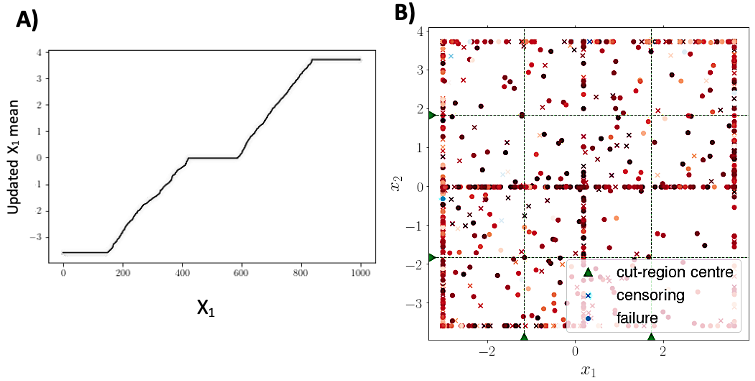
Figure 1: Simulation design for Scenario 3: Panel A illustrates a sample generated predictor mean, showcasing the construction of cut-regions where the effect of predictors gradually increases within specific intervals. Panel B provides an example of simulated data for Scenario 3, featuring two predictors, each with two cut-regions. Dots represent observed failure times, crosses indicate censoring times, and the colour gradient (red to blue) reflects the event/censoring times, with red representing earlier times and blue representing later times.

By incorporating these scenarios, our simulation study not only replicates prior work but also extends it to more realistic and challenging conditions, providing a robust evaluation of the methods under a wide range of data-generating processes.

4.2 Evaluation Metrics

We evaluated the performance of our proposed method, $Binacox+$ against $Binacox$ using the following criteria:

• Computation Time: We assessed the computational efficiency of $Binacox+$ and $Binacox$ across all three simulation scenarios to compare their scalability and runtime performance.

• Accuracy: In Scenario 1, where true cut-points exist, we evaluated the accuracy of the estimated cut-points using the $m_{1}$ accuracy metric proposed by Bussy et al. (2022). This metric calculates the Hausdorff distance between true and estimated cut-points only for predictors with at least one true and one estimated cut-point.

• Sparsity: In Scenario 2, which focuses on high-dimensional data with noise variables, we used the $m_{2}$ metric from Bussy et al. (2022) to evaluate the methods’ ability to distinguish truly associated predictors (with true cut-points) from noise variables (without true cut-points). The $m_{2}$ metric is defined as the proportion of predictors with at least one estimated cut-point relative to the number of predictors with at least one true cut-point.

• Model Performance: To evaluate the overall impact of the estimated cut-points on the fitted Cox models, we used two performance metrics: Akaike’s Information Criterion (AIC) and the Integrated Brier Score (IBS) in Scenario 3. These metrics assess the trade-off between model complexity and goodness-of-fit (AIC) and the accuracy of survival predictions (IBS), respectively.

To ensure the robustness and generalizability of our findings, we conducted simulations across five different sample sizes: 300, 500, 1000, 2000, and 4000. This allowed us to evaluate the scalability and reliability of the methods under varying data sizes. Each simulation configuration was repeated 500 times to ensure stable and reproducible results.

4.3 Simulation results

Figure 2 presents the average computational time (left) and the $m_{1}$ accuracy metric (right) for $Binacox+$ and $Binacox$ across different sample sizes ($n$) under Scenario 1. The results demonstrate that $Binacox+$ was consistently faster, with computation times ranging from 4 to 11 times shorter than $Binacox$, depending on the sample size. While the computing time for $Binacox+$ increased moderately with larger $n$, the computing time for $Binacox$ remained relatively constant, with a slight increase at $n=4000$. At the largest sample size ($n=4000$), $Binacox+$ was approximately 11 times faster than $Binacox$. In terms of the $m_{1}$ score, which measures the accuracy of estimated cut-points, $Binacox+$ consistently outperformed $Binacox$ across all sample sizes. The performance gap between the two methods was more pronounced at smaller sample sizes, underscoring the robustness of $Binacox+$ in data-limited settings.

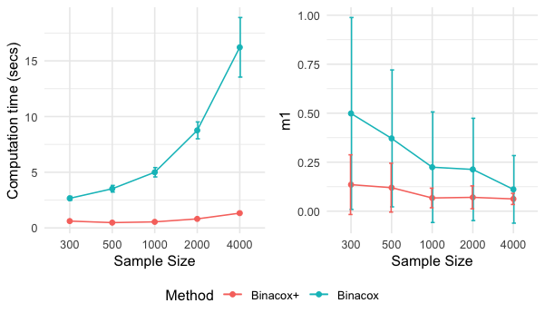
Figure 2: Comparison of $Binacox+$ (red) and $Binacox$ (blue) in the simulation Scenario 1: Average computing times in seconds (left) and average $m_{1}$ metric (right) across different sample sizes ($n$), with vertical lines representing ± the standard deviation (SD) based on 500 simulated datasets. The $m_{1}$ metric evaluates the accuracy of estimated cut-points, with lower values indicating better performance.

Figure 3 compares the methods in terms of average computational time (left) across different sample sizes, average computational time (middle) across varying numbers of features ($P$), and the $m_{2}$ sparsity metric (right) across different sample sizes under Scenario 2. Similar to Scenario 1, $Binacox+$ exhibited significantly shorter computation times compared to $Binacox$ across all sample sizes and values of $P$. The performance gap between the two methods widened with larger sample sizes and higher dimensionality. Additionally, $Binacox+$ achieved superior performance according to the $m_{2}$ sparsity metric, which evaluates the ability to distinguish truly associated predictors from noise variables. The difference in $m_{2}$ scores between the two methods was more pronounced at smaller sample sizes, further highlighting the advantages of $Binacox+$ in high-dimensional settings.

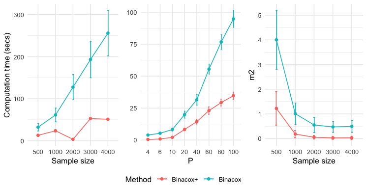
Figure 3: Performance of $Binacox+$ (red) and $Binacox$ (blue) in the simulation Scenario 2: Average computing times in seconds across different sample sizes ($n$, left) and varying numbers of features ($P$, middle), along with the average $m_{2}$ metric (right) for sparsity evaluation. Vertical lines represent ± the standard deviation (SD) based on 500 simulated datasets. The $m_{2}$ metric measures the proportion of predictors with at least one estimated cut-point relative to those with true cut-points, with higher values indicating better performance.

Figure 4 displays the average computation times (left), average AIC (middle), and average IBS (right) for the fitted Cox models under Scenario 3. The predictors for these models were categorized using the cut-points estimated by $Binacox+$ and $Binacox$. For comparison, we also included the “true” model, which used the original continuous predictors. Consistent with the previous scenarios, $Binacox+$ demonstrated superior computational efficiency compared to $Binacox$ across all sample sizes. In terms of model performance, all three models ($Binacox+$, $Binacox$, and the “true” model) achieved similar AIC and IBS values, indicating that both methods effectively captured the underlying relationships between predictors and outcomes, even in the absence of true cut-points. This suggests that $Binacox+$ and $Binacox$ are capable of approximating the true data-generating process through categorization, despite the added complexity of cut-regions in Scenario 3.

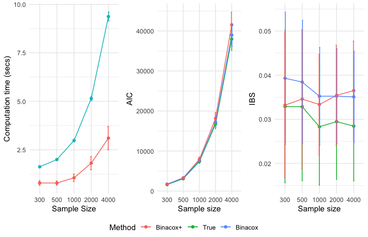
Figure 4: Performance of $Binacox+$ (red) and $Binacox$ (blue) in the simulation Scenario 3: Average computing times in seconds (left), average Akaike’s Information Criterion (AIC, middle), and average Integrated Brier Score (IBS, right) across different sample sizes ($n$). As reference, the “true” model, which used the original continuous predictors, is added (in green) to the AIC and IBS plots. Vertical lines represent ± the standard deviation (SD) based on 500 simulated datasets.

5 Case study

5.1 Datasets

To evaluate the practical performance of our method, we applied both $Binacox+$ and $Binacox$ to three biomedical datasets from The Cancer Genome Atlas (TCGA) platform, which were previously used by Bussy et al. (2022). These datasets include breast invasive carcinoma (BRCA), glioblastoma multiforme (GBM), and kidney renal clear cell carcinoma (KIRC). TCGA is a publicly available resource that leverages genomic technologies, such as large-scale genome sequencing, to advance the understanding of cancer’s molecular basis. Since their use in Bussy et al. (2022), these datasets have been updated significantly. The most recent versions include 1,231 patients for BRCA, 391 patients for GBM, and 614 patients for KIRC, each with both gene expression and survival data. The gene expression data consist of Fragments Per Kilobase per Million mapped fragments (FPKM) unstrand values for 60,660 genes.

Following the approach of Bussy et al. (2022), we performed an initial screening step by fitting a Cox model for each gene individually and calculating the Akaike Information Criterion (AIC) and Integrated Brier Score (IBS) for each model. Genes were then ranked based on these metrics, and the top 50 genes from each ranking were selected, resulting in up to 100 unique genes per dataset (due to overlap between the top 50 genes from each metric). Finally, the selected genes were standardized before applying $Binacox+$ and $Binacox$. A summary of the datasets after the screening step is provided in Table 1.

Table 1: Summary of the breast invasive carcinoma (BRCA), glioblastoma multiforme (GBM), and kidney renal clear cell carcinoma (KIRC) datasets obtained from The Cancer Genome Atlas (TCGA) after the initial screening step including the number of patients, the total number of genes, and the number of genes selected for analysis after ranking based on Akaike’s Information Criterion (AIC) and Integrated Brier Score (IBS).

Dataset	n	Total no. of genes	No. of selected genes
BRCA	1231	60660	99
GBM	391	60660	94
KIRC	614	60660	95

5.2 Estimated cut-points

We applied both $Binacox+$ and $Binacox$ to each dataset after the screening step. Table 2 reports the estimated cut-points for the GBM dataset. $Binacox+$ detected a single cut-point for 13 genes and two cut-points for 3 genes in this dataset. The estimated cut-points for the BRCA (1 gene) and KIRC (13 genes) datasets are detailed in Tables 4 and 5 in the Supplementary Materials. In contrast, $Binacox$ failed to detect any cut-points for the GBM and BRCA datasets and identified a single cut-point for 16 genes in the KIRC dataset, none of which overlapped with those detected by $Binacox+$.

Table 2: Estimated optimal cut-points for the GBM dataset identified by $Binacox+$ and $Binacox$. The table summarizes the number of genes with detected cut-points, including single and multiple cut-points, as well as their specific values.

Genes	$Binacox+$	$Binacox$
LINC00906	-0.32	.
AC083906.5	-0.79	.
CPPED1	-1.43	.
LBH	-1.01	.
AC090114.1	-1.01	.
SNRPB	-1.07	.
PTPRN2	-1.15	.
AC008875.3	-1.33, -1.18	.
CYB561	-1.48	.
PODNL1	-0.52	.
HPCAL1	-1.12, -1.03	.
RNF175	-1.08	.
AC073332.1	-1.01	.
CLEC5A	-1.04, -0.99	.
AL592064.1	-0.34	.
PLK2	-1.07	.

5.3 Model performance

To evaluate the impact of the detected cut-points on the overall performance of the Cox model, we categorized genes with at least one detected cut-point for each method and fitted Cox models using these categorized predictors. Table 3 summarizes the performance metrics, including AIC, IBS, and the Concordance Index (C-index) along with its estimated SD, for the fitted Cox models based on the categorized gene expression predictors for both $Binacox+$ and $Binacox$. $Binacox+$ consistently outperformed $Binacox$ across all three datasets, achieving the lowest AIC and IBS values and the highest C-index values.

Table 3: Performance metrics for Cox models fitted using categorized gene expression predictors derived from the estimated cut-points of $Binacox+$ and $Binacox$. The table presents Akaike’s Information Criterion (AIC), Integrated Brier Score (IBS), and Concordance Index (C-index) with its estimated standard deviation (SD) for each method across the BRCA, GBM, and KIRC datasets. Lower AIC and IBS values indicate better model fit and predictive accuracy, respectively, while a higher C-index reflects superior discriminative performance.

Dataset	Metric	$Binacox+$	$Binacox$
BRCA	AIC	2080.2	2108.8
BRCA	IBS	0.157	0.163
BRCA	C-index (SD)	0.548 (0.015)	0.5 (0)
GBM	AIC	2853.4	3026.7
GBM	IBS	0.044	0.064
GBM	C-index (SD)	0.726 (0.016)	0.5 (0)
KIRC	AIC	2065.2	2166.5
KIRC	IBS	0.146	0.182
KIRC	C-index (SD)	0.769 (0.016)	0.698 (0.018)

6 Discussion

In this paper, we introduced $Binacox+$, an enhanced version of the $Binacox$ method, designed for rapid and accurate estimation of multiple cut-points in Cox models with high-dimensional features. Through extensive simulation studies, we demonstrated that $Binacox+$ significantly outperforms the original $Binacox$ method, achieving computational speeds up to 11 times faster while maintaining superior performance in cut-point detection and model accuracy. Notably, $Binacox+$ excels in identifying multiple cut-points per feature, a critical capability for modelling complex relationships in high-dimensional data. We further validated its practical utility by applying it to three publicly available high-dimensional genetic datasets, showcasing its effectiveness in real-world applications.

The cumulative binarization approach used in $Binacox+$ addresses several limitations of conventional binarization methods for categorizing continuous covariates. Traditional binarization methods, which rely on fixed intervals or percentiles, are often sensitive to the choice of interval boundaries and can lead to small sample sizes in certain bins, reducing statistical power and introducing bias (Royston et al., 2006). In contrast, the nested intervals in $Binacox+$ are less sensitive to boundary choices, allowing for more flexible and precise cut-point estimation without compromising sample size. This approach mitigates issues such as residual confounding and loss of precision, particularly in the outer intervals of the data range (Naggara et al., 2011).

However, our study has some limitations. First, the performance of $Binacox+$ relies on the pre-specified set of cut-point candidates, which may not always capture the true underlying structure of the data. Second, while $Binacox+$ is computationally efficient, its scalability to ultra-high-dimensional datasets (e.g., millions of features) remains to be tested. Finally, the method assumes that the relationship between predictors and outcomes can be adequately modelled using cut-points, which may not hold for all types of data. Future work could explore adaptive methods for selecting cut-point candidates and extend $Binacox+$ to handle more complex data structures.

How can this approach be utilized in real-world applications? We strongly advocate for first identifying the optimal relationship between predictors and the risk of outcomes, irrespective of its immediate clinical interpretability. This can be achieved using an additive Cox proportional hazards model, such as the Cox-based Generalized Additive Model (CGAM), which leverages smoothing spline-based machine learning algorithms (Hastie and Tibshirani, 1990; Wood et al., 2016; Bender et al., 2018). In this approach, continuous predictors are included in the Cox model, and smoothing splines are applied to flexibly estimate potentially non-linear, data-driven relationships between predictors and outcomes. Generalized cross-validation can be used during model fitting to determine the appropriate level of smoothness, thereby avoiding overfitting while maintaining flexibility.

For generating clinically actionable insights, we recommend using $Binacox+$ to categorize continuous predictors based on identified cut-points and fitting a standard Cox proportional hazards model. This approach balances interpretability and performance, making it more suitable for practical applications. To evaluate the trade-off between interpretability and predictive accuracy, model performance metrics such as AIC or IBS can be used to compare the simplified Cox model with the more flexible CGAM. This ensures that the results remain both scientifically robust and clinically relevant.

In conclusion, $Binacox+$ represents a significant advancement in the analysis of high-dimensional survival data, offering a computationally efficient and interpretable approach for identifying multiple cut-points per feature. Its ability to handle complex relationships while maintaining high predictive accuracy makes it a valuable tool for both research and clinical applications. By combining the flexibility of non-parametric methods with the simplicity of categorized predictors, $Binacox+$ bridges the gap between statistical rigour and practical usability, paving the way for more effective prognostic modelling in high-dimensional settings. Future research should focus on extending its applicability to ultra-high-dimensional data and exploring adaptive methods for cut-point selection to further enhance its utility.

Supporting Information

Table 4: Estimated optimal cut-points for the BRCA dataset identified by $Binacox+$ and $Binacox$. The table summarizes the number of genes with detected cut-points, including single and multiple cut-points, as well as their specific values.

Genes	$Binacox+$	$Binacox$
ABCB5	-0.42	.

Table 5: Estimated optimal cut-points for the KIRC dataset identified by $Binacox+$ and $Binacox$. The table summarizes the number of genes with detected cut-points, including single and multiple cut-points, as well as their specific values.

Genes	$Binacox+$	$Binacox$
CUBN	-1.01	.
TXLNA	-1.58	.
NUMBL	-0.88	.
CYP3A7	-0.52	.
EIF4EBP2	-1.63	.
SORBS2	-1.71	.
ANAPC7	-1.19	.
SLC16A12	-1.11	.
CDCA3	-0.59	.
SLC2A9	-0.95	.
HJURP	-0.60	.
IL4	-0.77	.
CARS1	-1.45	.
RUNDC3B	.	-1.05
GGACT	.	-0.48
SEMA3D	.	-0.62
KMT5A	.	-1.43
Z83745.1	.	-0.87
PTPRB	.	-1.32
GIPC2	.	-1.37
FBXL5	.	-1.45
EHHADH	.	-1.23
AMOT	.	-1.45
MSH3	.	-1.31
OSBPL1A	.	-1.65
PLPP3	.	-1.44
SLC52A2	.	-1.11
RORA	.	-1.22
METTL24	.	-1.13

References

- Alaya et al. (2019) Alaya, M., Bussy, S., Gaiffas, S., and Guilloux, A. (2019). Binarsity: a penalization for one-hot encoded features in linear supervised learning. Journal of Machine Learning Research 20, 1–118.
- Bender et al. (2018) Bender, A., Groll, A., and Scheipl, F. (2018). A generalized additive model approach to time-to-event analysis. Statistical Modelling 18, 299–321.
- Bennette and Vickers (2012) Bennette, C. and Vickers, A. (2012). Against quantiles: categorization of continuous variables in epidemiologic research, and its discontents. BMC Medical Research Methodology 12, 12–21.
- Bland and Altman (1995) Bland, M. and Altman, D. (1995). Multiple significance tests: the bonferroni method. BMJ 310, 170.
- Bussy et al. (2022) Bussy, S., Alaya, M., Jannot, A.-S., and Guilloux, A. (2022). Binacox: automatic cut-point detection in high-dimensional cox model with applications in genetics. Biometrcs 78, 1414–1426.
- Cheang et al. (2009) Cheang, M., Chia, S., Voduc, D., Gao, D., and et al. (2009). Ki67 index, her2 status, and prognosis of patients with luminal b breast cancer. Journal of National Cancer Institute 101, 736–750.
- Cox (1972) Cox, D. (1972). Regression models and life-tables. Journal of the Royal Statistical Society 34, 187–202.
- Gaïffas and Guilloux (2012) Gaïffas, S. and Guilloux, A. (2012). High-dimensional additive hazards models and the Lasso. Electronic Journal of Statistics 6, 522 – 546.
- Hastie and Tibshirani (1990) Hastie, T. and Tibshirani, R. (1990). Generalized Additive Models. Chapman & Hall/CRC.
- Lausen and Schumacher (1992) Lausen, B. and Schumacher, M. (1992). Maximally selected rank statistics. Biometrics 48, 73–85.
- Moeschberger and Klein (2005) Moeschberger, M. L. and Klein, J. P. (2005). Survival analysis: techniques for censored and truncated data. Amsterdam: Springer Science & Business Media.
- Naggara et al. (2011) Naggara, O., Raymond, J., Guilbert, F., Roy, D., Weill, A., and Altman, D. (2011). Analysis by categorizing or dichotomizing continuous variables is inadvisable: An example from the natural history of unruptured aneurysms. American Journal of Neuroradiol 32, 437–440.
- Nath Mukhexjee and Samar Maiti (1988) Nath Mukhexjee, B. and Samar Maiti, S. (1988). On some properties of positive definite toeplitz matrices and their possible applications. Linear Algebra and its Applications 102, 211–240.
- Royston et al. (2006) Royston, P., Altman, D., and Sauerbrei, W. (2006). Dichotomizing continuous predictors in multiple regression: a bad idea. Statistics in Medicine 25, 127–141.
- Safari et al. (2024) Safari, A., Helisaz, H., Salmasi, S., Adelakun, A., De Vera, M., and et al. (2024). Association between oral anticoagulant adherence and serious clinical outcomes in patients with atrial fibrillation: A long‐term retrospective cohort study. Journal of the American Heart Association 13, e035639.
- Salmasi et al. (2024) Salmasi, S., Safari, A., De Vera, M., Hogg, T., and et al. (2024). Adherence to direct or vitamin k antagonist oral anticoagulants in patients with atrial fibrillation: a long-term observational study. Journal of Thrombosis and Thrombolysis 57, 437–444.
- Wood et al. (2016) Wood, S., Pya, N., and Safken, B. (2016). Smoothing parameter and model selection for general smooth models. Journal of the American Statistical Association 111, 1548–1563.
- Wu and Coggeshal (2012) Wu, J. and Coggeshal, S. (2012). Foundations of Predictive Analytics. Chapman and Hall/CRC.