Spatial Data Science Languages: commonalities and needs

Abstract

Recent workshops brought together several developers, educators and users of software packages extending popular languages for spatial data handling, with a primary focus on R, Python and Julia. Common challenges discussed included handling of spatial or spatio-temporal support, geodetic coordinates, in-memory vector data formats, data cubes, inter-package dependencies, packaging upstream libraries, differences in habits or conventions between the GIS and physical modelling communities, and statistical models. The following set of insights have been formulated: (i) considering software problems across data science language silos helps to understand and standardise analysis approaches, also outside the domain of formal standardisation bodies; (ii) whether attribute variables have block or point support, and whether they are spatially intensive or extensive has consequences for permitted operations, and hence for software implementing those; (iii) handling geometries on the sphere rather than on the flat plane requires modifications to the logic of simple features, (iv) managing communities and fostering diversity is a necessary, on-going effort, and (v) tools for cross-language development need more attention and support.

1 Introduction

High-level open-source programming languages for data science enable users to combine data management, interactive data analysis, and application development in a single environment. R [R Core Team, 2023], Python [Van Rossum et al., 2007] and Julia [Bezanson et al., 2017] dominate in this space. Spatial data science in these languages is the focus of this paper. A growing focus on ‘open science’ principles and reproducibility in scientific research have further increased the demand for these languages [Hughes-Noehrer et al., 2024]. A notable domain is that of spatial data science, which focusses on datasets with explicit spatial locations. It is used in many applied fields, including climate, oceanography, agriculture, ecology, biodiversity, geography, and mobility. Analysis tasks range from data collection and cleaning, combining different datasets, exploring data, visualising it, predicting new observations to statistical inference and identifying outliers or causalities.

R has the oldest roots of the three languages considered in this paper, dating back to the mid 1970s [Becker et al., 1986]. R grew out of an experimental project to make an alternative implementation of the statistical programming language S. In the 1997, R was open-sourced, and by the early 2000s had largely replaced S and S-Plus in academia. Spatial R packages have a history dating back to their development as S-Plus extensions. Early attempts to handle spatial data were initiated by Roger Bivand, and reported in Pebesma and Bivand [2005]. A coherent group of packages for spatial statistics was described in Bivand et al. [2013], the first edition of which appeared in 2008. Interface packages rgdal [Bivand et al., 2017] and rgeos were retired in 2023, as they had been superseded by sf [Pebesma, 2018, Pebesma and Bivand, 2023], a package that is standards-based and uses modern interfaces like Rcpp [Eddelbuettel, 2013] and tidyverse [Wickham et al., 2019].

Python was released in 1991 but its tooling for spatial data science evolved much later. The foundation of the ecosystem we use today can be linked to the work of Butler and Gillies [2005] eventually resulting in the release of Shapely [Gillies et al., 2023b] as the Python bindings of GEOS in 2007, Rtree [Butler et al., 2023] as bindings of libspatialindex in the same year and Fiona [Gillies et al., 2023a] as bindings of GDAL managing vector geometries in 2008. Raster bindings through the rasterio [Gillies et al., 2013–] package came five years later in 2013. The PROJ bindings, known as pyproj [Snow et al., 2023] are around since 2006. In parallel, the work of Anselin et al. [2006] within the GeoDA/PySpace and that of Rey and Janikas [2006] in STARS have merged and formed the Python Spatial Analytics Library (PySAL) [Rey and Anselin, 2007], at the time not tied to any of the bindings mentioned above. The modern ecosystem is much more connected and oftentimes revolves around the GeoPandas package [den Bossche et al., 2023], released in 2013 to provide a common data frame-based interface to all Shapely, Rtree, and Fiona. In the recent years, PySAL is progressing towards closer dependence on the GeoPandas-based ecosystem and deprecating its own geometry classes and file interfaces. The world of raster data has been evolving largely in parallel based heavily on rasterio and numpy [Harris et al., 2020], with modern tools embracing xarray [Hoyer and Hamman, 2017] and the general Pangeo ecosystem.

Julia, introduced in 2012 and version 1.0 released in 2018, is a relatively young programming language [Bezanson et al., 2017]. Its spatial tools have also emerged recently. Initially, efforts focused on wrapping C libraries like GDAL.jl and LibGEOS.jl, facilitated by Julia’s call interface, automatic wrapper packages such as Clang.jl, and its built-in package manager that supports binary dependencies. These foundational packages have been abstracted to simplify working with C libraries. More recently, higher-level abstractions like Rasters.jl and GeoDataFrames.jl have been developed, allowing for one-liner operations. With many Julia packages incorporating (some form of) geometry, a spatial interface package called GeoInterface.jl was created to enable spatial interoperability and conversion between different packages using traits. The latest developments leverage Julia’s ability to compile high-performance native code, leading to the implementation of spatial algorithms directly in Julia, such as GeometryOps.jl, rather than relying on the GEOS wrapper.

Each programming language is characterised by communities in which the exact boundary between developers and users is blurred: users need to write commands to get something done, and many users get into development sooner or later because they need to, and find out they can. Other programming languages like JavaScript, Java and Rust have also thriving communities working on spatial data, but have a stronger division between users and developers. These latter languages, as well as the older languages Fortran, C and C++ have important components for spatial data analysis that are often interfaced using binary language bindings and thus also become useful to R, Python and Julia users. All three languages use a common representation for vector geometries defined by the simple feature access standard [Herring, 2011]. Additionally, each language has infrastructure to read diverse data types such as raster (imagery), spatio-temporal array data (data cubes), and more traditional vector data formats as well as ways to interface with spatial databases, such as PostGIS and Spatialite with their built-in spatial analysis functions.

In September 2023, a hybrid Spatial Data Science across Languages (SDSL) workshop was organised by Edzer Pebesma at the Institute for Geoinformatics of the University of Münster. In September 2024, a second edition was organised by Martin Fleischmann at the Charles University. These workshops served as a collaborative platform for developers, educators, and users of software packages extending R, Python, and Julia. The events were focused on addressing the challenges related to the handling and analysis of spatial data. They fostered discussions among experts in the field, leading to the identification of common challenges and formulation of a set of recommendations, described in this document, aimed at limiting potential pitfalls in spatial data analysis, cultivating communication between groups of developers and users, and enhancing the capabilities of spatial data science software.

2 Common challenges

2.1 File formats, data connectivity, and in-memory representation

A commonality across the spatial data science languages considered is that each has a diverse and modular ecosystem of composable packages/functions that can be mixed and matched to provide highly customizable in-memory transformations compared to a traditional desktop GIS-based processing workflow. Whereas desktop GIS-based processing workflows typically combine tools that read files as input and write files as output, spatial data science language workflows commonly combine tools that transform data frames containing one or more columns with a geometry data type.

Because many spatial data science workflows depend heavily on data frame transformations, libraries in these languages are closely related to the respective data frame libraries: GeoPandas is an extension of the pandas data frame library in Python; sf is built on R’s built-in data.frame and provides methods for tidyverse-style transformations, and GeoDataFrames.jl is built on top of the DataFrames.jl package in Julia. All of these add the concept of a ”primary geometry column” and propagate its identity through as many transformations as possible. Similarly, columnar geometry representations in R, Julia, and Python treat CRS as a column-level concept and propagate/validate its value wherever possible.

In-memory geometry column representation and examples of sharing between packages is accomplished: In R, this is achieved with sf and sfc object classes, and some example tools that leverage the ABI-stable (application binary interface) memory model are exactextractr, stars, geojsonsf. In Julia, this is GeoInterface.jl, or a set of traits/generic methods that other packages can use to write generic algorithms to read or transform an arbitrary geometry source. In Python, this is a numpy array of Shapely objects, which are wrappers around GEOS geometries.

Since the development of geospatial support in R, Julia, and Python, the diversity of tools available to work with data frames has exploded: Polars, DuckDB, cuDF, and Apache Arrow all offer some level of accelerated data frame transformation in Python with varying levels of support in R and Julia. As data size increases, users increasingly reach for these tools and file formats such as Parquet that scale to support larger-scale spatial workflows.

Efforts to extend these libraries and formats to integrate with the larger spatial ecosystem are underway: the OGC GeoParquet 1.1.0 specification was recently released [Holmes et al., 2024] to extend the Parquet format to mark columns as geometry and propagate the primary geometry column, while Apache Parquet specification itself recently included native support for geometry and geography columns [Dem et al., 2025], which will be used by GeoParquet 2.0.0. The GeoArrow 0.1.0 specification [Dunnington et al., 2024], also recently released, includes both Apache Arrow extension types (enabling first-class support for a geometry type in Arrow-based tools) and efficient memory layouts compatible with DuckDB [Raasveldt and Muehleisen, ], Polars [Vink et al., 2025], cuDF [Team, 2023], and Parquet. DuckDB and cuDF both have geospatial extensions and work is underway to improve connectivity and metadata propagation among geometry representations in these libraries and geometry representations in spatial data science ecosystems.

A commonality across the spatial data science languages considered is that a typical workflow starts with reading data from an external data source, like a file or database connection, compute, and write results which may be a figure or again data written to some file. A lot of interest has recently gone into efficient handling (reading, analysing, writing) of large vector and raster data, in combination with cloud computing. For vector data, ”classic” file formats such as Esri Shapefile or GeoPackage organize data record by record; for many analytical purposes columnar storage formats such as GeoParquet can be considerably faster. In-memory data representations such as GeoArrow, or those used by DuckDB or Polars can also speed up processing and avoid copying of large amounts of data. Spatial tiling such as done in FlatGeobuf or PMTiles may speed up reads of particular regions. The growth and popularity of Apache Arrow as a common in-memory interchange representation is reflected in GDAL, which optionally enabled reading of vector file formats as an Arrow table in the version 3.6, followed by the write support and inclusion of the GeoArrow specification two releases later. This allows performant bulk I/O tailored to data frame representations of spatial data.

Apache Arrow, together with its GeoArrow extension, has a potential to change the way we move spatial data between different languages as Arrow can serve as an in-memory representation that can be accessed without copying from R, Python, Julia, Rust, C++, JavaScript, and others. Given other languages like Rust or JavaScript can also directly consume Arrow data, efficient support of Arrow should be a priority across all high-level languages.

For raster data and data cubes, formats such as Zarr and cloud-optimized GeoTIFF (COG) are frequently used; these allow for tiling, chunked reads, region reads, and low resolution / strided reads. Such formats often require additional libraries like BLOSC and LERC for compressing scientific (floating point) data.

2.2 Inter-package dependencies and shared upstream libraries

One of the powerful features of modern languages is that they can be extended by packages that are developed and distributed by the community. Such package may reuse other packages, allowing developers to build-on the work of others and focus on things they know well. Important tasks like reading and writing to external data formats, geometrical operations and conversions or transformation of coordinates is typically left to external libraries that are shared by a much larger open source community.

2.2.1 Inter-package dependencies across languages

A common feature of each language’s support for spatial data is using existing low-level libraries for fundamental operations such as data import, export, and coordinate system transformation. This approach is efficient because it avoids reinventing the wheel, but does mean that ’system dependencies’ need to be managed somehow. Each language needs to have access to GDAL binaries, for example, and this is currently handled differently in each language. Figure 1 gives an overview how the main geospatial R and Python packages depend on a common set up upstream C/C++ libraries.

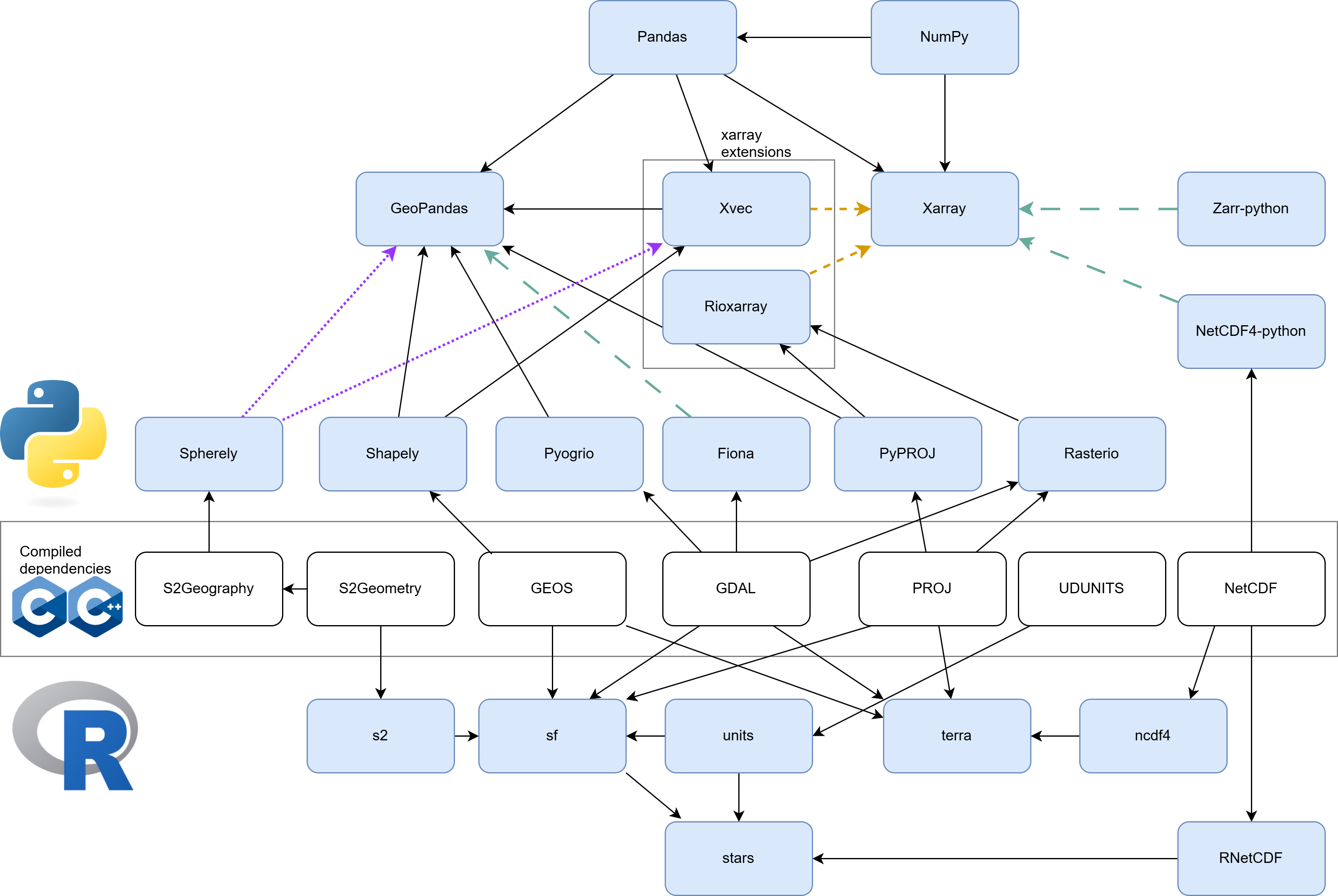
Figure 1: Dependency of R and Python spatial packages on other libraries and external system requirements. Green long-dashed arrows indicate optional dependencies, purple dotted arrows indicate planned optional dependencies, while the orange dashed lines indicate optional dependency through the Xarray’s extension mechanism.

In R, pre-built binary packages provided by the Comprehensive R Archive Network (CRAN) for Windows and Mac contain the system requirements: libraries such as GDAL, PROJ, UDUNITS and S2Geometry are compiled and statically linked to the shared library contained in the package. This leads to some duplication and inflexibility to upgrade system requirements by users, but has the advantage that binary packages, after installation, ”just work”. Linux users who install source packages must first install the system requirements, unless the package contains (”vendors”) the complete library (as s2 and GEOS do). Linux binary distributions of packages are also available, typically use dynamic linking and thus make implicit, hard requirements to installed versions; examples are r2u, Posit Public Package Manager and bspm.

In Python, GeoPandas depends on Shapely to provide GEOS bindings, either on Fiona or Pyogrio to provide GDAL bindings and on pyproj to interface PROJ. In future, this list will also include Spherely, providing bindings to S2Geometry. The dependency on compiled C++ libraries and a resulting need for compiled distributions of Python packages directly depending on them may occasionally bring additional friction into the installation process. Historically, not all packages had released versions for all operating systems (often excluding Windows), which lead to the growth of independent community-led packaging efforts like conda-forge [conda-forge community, 2015] aiming to solve the packaging process by cross-compiling all packages in the ecosystem, ensuring binary compatibility and cross-platform support.

Like the other languages, Julia wraps the C bindings of GDAL, GEOS and PROJ libraries. However this is done in a generic way to produce versioned, shared binaries for the whole ecosystem. It does so by first cross-compiling all these projects, including all their (inter)dependencies as an artefact package (a so called .jll package, compared to normal .jl usage for a pure Julia package) for fourteen common platforms and application binary interfaces (ABIs). Packages like GDAL.jl then depend on GDAL_jll and wrap the C statements in Julia calls. Furthermore julian—abstractions have been build on top, such as ArchGDAL.jl, then Rasters.jl and GeoDataFrames.jl on top of that. In Julia it is easy to create new packages and extend functionality of other packages and types. This focus on composability has lead to an emphasis on interfaces, as seen in Figure 2.

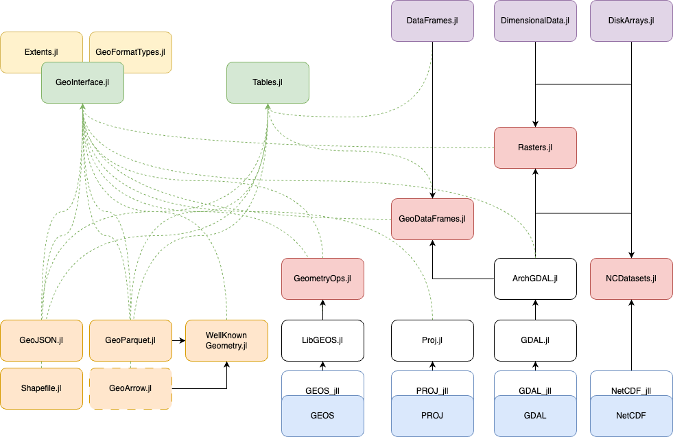
Figure 2: Geospatial stack in Julia. Like other languages, the well known C++ libraries are wrapped (blue), resulting in the core packages of GeometryOps.jl, GeoDataFrames.jl, and Rasters.jl (red). A number of packages implement native file formats (orange). Note that while the stack depends on other non-spatial Julia packages (purple), much of the interaction and indeed dependencies are replaced by the implementation of interfaces using traits (green). Only where native Julia types are not adequate, we created spatial versions of them (yellow).

2.3 Polygonal coverage

In most of the cases discussed above, polygon data describe a partitioning (tessellation) of the domain of interest, meaning that no two polygons overlap and all area of interest is covered. This refers to polygon coverage (for point support variables) or choropleth (for block support variables). Knowing that a dataset represents a valid polygonal coverage brings significant benefits to the subsequent processing as the algorithms depending on overlay relations can avoid the need of testing the relationship beyond the ”touches” predicate. Furthermore, a valid coverage ensures that vertices reflecting shared edges are present in both neighbouring polygon, enabling fast coordinate-based construction of contiguity matrices representing which polygon neighbours which. Yet, the simple feature standard [Herring, 2011] ignores this, and users are typically faced with a set of polygon rings without any guarantee. Having tools to verify overlaps, or to identify and remove small, unwanted gaps or overlaps resulting from careless, topology-ignoring line simplification would be convenient since geometrical operations become more efficient when it is known that polygons do not overlap. This is currently available only in a rather prototypical form.

2.3.1 Polygonal coverage across languages

GEOS, as of version 3.13.0, offers coverage validation and coverage gap finding to support its coverage-based algorithms for simplification and union but not tooling for coverage enforcement and correction. In Python, the package geoplanar [Rey et al., 2023], covering most of the common planarity violations and their correction, attempts to fill this gap. We are not aware of other attempts in R or Julia but users occasionally rely on JavaScript library mapshaper [Bloch, 2024], offering experimental tooling for topology cleaning, or GRASS GIS [GRASS Development Team, 2024].

2.4 Geodetic coordinates, spherical geometry

Geodetic coordinates (also known as Geographic or Geographical coordinates), degrees longitude and latitude describing points on an ellipsoid or sphere, are fundamentally different from Cartesian coordinates describing points on a flat surface. For simplicity we will ignore here that the Earth’s shape is better approximated by an ellipsoid rather than a sphere, not because this is not important but because the difference between sphere and ellipsoid is much smaller than between a sphere and a flat surface. With the increasing availability of global datasets, we also see an increase in datasets with geodetic coordinates.

For geodetic coordinates with longitude $\lambda$ and latitude $\phi$, the two points POINT($\lambda=0$ $\phi=90$) and POINT($\lambda=90$ $\phi=90$) coincide, as do the two points POINT($\lambda=-180$ $\phi=30$) and POINT($\lambda=180$ $\phi=30$). For Cartesian coordinates, swapping the $x$ and $y$ coordinate results in identical distance computations but that is not the case for geodetic coordinates. Geodetic coordinates measure angles and have units in degrees, Cartesian coordinates measure distance and have length units.

There is a long tradition in geospatial data analysis and GIS to treat geodetic coordinates as if they are Cartesian [Chrisman, 2012], which corresponds to using the so-called plate carrée projection, in which $x=\lambda,y=\phi$. As an example, the GeoJSON specification [Butler et al., 2016] prescribes to handle all geodetic coordinates as Cartesian in the rectangle bound by POINT($x=-180$ $y=-90$) and POINT($x=180$ $y=90$). This may be helpful for some problems, but not for others, and one wonders how many users of GeoJSON are aware of these explicit intentions.

As an alternative, one might consider geodetic coordinates as coordinates on a sphere. This, however, changes a number of fundamental things. For example, on a flat surface, any ring has an unambiguous inside and an outside: only one of them has a finite surface. A sphere, by contrast, is a finite surface and any ring (polygon), therefore, divides the sphere’s surface into two finite parts.

Similarly, on a flat surface, one can use the terms ”clockwise” (CW) and ”counter-clockwise” (CCW) to indicate the winding order of the nodes of a ring; on the sphere this is again ambiguous: if one takes the ring formed by the equator, CW and CCW flip when one changes the side from which one looks at it.

Another issue is that straight lines are unambiguously straight on a flat surface but, on a sphere, they are curved; the obvious choice is to use great circles arcs (the shortest path over the sphere connecting two points). Great circle arcs do not coincide to straight lines in the plate carrée view [Butler et al., 2016], except when they fall on a meridian or the equator.

When using the simple features standard to handle polygons on the sphere [Herring, 2011], one needs to additionally take care of:

• winding order: simple features require outer rings to have CCW, inner rings (holes) to have CW winding, but this is not enforced and most software does not require this (e.g. GEOS produces geometry with reversed windings). The options are either to define the inside of a ring to be the area to the left when following nodes, or more pragmatically define the inside as the smaller of the two polygons,

• the POLYGON FULL: the special polygon formed by the entire Earth’s surface as the negation of the empty set, POLYGON EMPTY,

• validity: polygons valid on plate carrée are not generally valid on the sphere, and vice versa [Pebesma and Bivand, 2023].

2.4.1 Geodetic coordinates across languages

The R package sf has, since its 1.0-0 release in June 2020 adopted the s2 package, which wraps the S2Geometry C++ library to fully use spherical geometry operations by default when provided coordinates are geodetic.

The Python package GeoPandas aims to follow the behaviour of the R package sf and leverage the S2Geometry C++ library when dealing with spherical data. The work to create vectorized Python bindings to S2Geometry enabling this is currently ongoing within the Spherely package and it is expected that the first experimental support of spherical geometry in GeoPandas will be released in upcoming versions. So far, however, GeoPandas shows a warning like in the example below where a GeoDataFrame with geographic coordinates is queried for polygon areas. The ”units” of the values obtained are ”squared degrees”. For area, this is not helpful as an area of 1°$\times$ 1° is over 12000 km² near the equator, whereas near the poles it is a bit over 100 km². See the treatment of geodetic coordinates in GeoPandas 0.14:

⬇

>>> import geopandas

>>> countries = geopandas.read_file(”countries/”)

>>> countries.area

<stdin>:1: UserWarning: Geometry is in a geographic CRS. Results from ’area’ are likely incorrect. Use ’GeoSeries.to_crs()’ to re-project geometries to a projected CRS before this operation.

0 1.639511

1 76.301964

2 8.603984

3 1712.995228

4 1122.281921

…

172 8.604719

173 1.479321

174 1.231641

175 0.639000

176 51.196106

Length: 177, dtype: float64

The warning message emitted by GeoPandas is correct, but one wonders how often data scientists seeing it will follow the advice, as the warning does not suggest a concrete coordinate reference system to use in to_crs(). For area computations, one could choose an equal area projections, transform the data, and recompute area. The problem is harder for distance computations, or e.g. computing buffers involving global or near-global datasets. In such cases, projection to Cartesian coordinates is not a great solution, and computations on a spherical (or ellipsoidal) geometry are to be preferred.

In Julia, most packages implicitly assume operations are based on Cartesian coordinates. Because not all geometries include a coordinate reference system (CRS) or can determine if the attached CRS is geodetic, the software cannot alert users, leaving them to verify the correctness of operations themselves. Some packages offer partial support for geodetic operations, such as calculating great circle distances, or provide workarounds like a cellsize method to accurately compute raster areas.

Since the first SDSL workshop, the GeoInterface.jl package has introduced a crstrait trait, allowing packages to identify the CRS type and automatically select the appropriate method when available. This trait is currently being integrated across the ecosystem. Additionally, efforts are underway to wrap the S2Geometry library in Julia, aiming to offer a comprehensive suite of geodetic operations.

Writing spatial data to dedicated file formats needs care if coordinate reference systems are not specified. Writing GeoPackage files with GDAL ($\geq 3.9$) without specifying a CRS creates a file that, upon reading, specifies that coordinates are geodetic. A dedicated layer creation options (SRID="99999") or a dedicted WKT specification of an unknown engineering CRS specifies Cartesian coordinates, the default assumption in sf and GeoPandas for objects without specified CRS. GeoParquet also has a metadata flag that specifies whether line or polygon edges should be taken linear (Cartesian) or great circle arcs (geodetic). Some file formats (e.g., GeoPackage, GeoParquet, Parquet) interpret a missing CRS as having geodetic coordinates.

2.5 Maps

Among all statistical graphs, maps are compelling because it is so easy to relate to them. Yet, any map is a projection and creating code that maps unprojected data involves choosing defaults: should the projection preserve area, should Europe be at the center of the map, should North point up, should a graticule (a grid with lines following constant longitude or latitude) be added?

Currently, the default plot method of R package sf uses an equidistant rectangular projection, meaning that longitude and latitude are mapped linearly to $x$ and $y$, with unit scale (one unit distance in $x$ direction equals one unit distance in $y$ direction) at the center of the map. GeoPandas applies the same treatment when dealing with unprojected data. Other software may choose for a plate carrée projection (e.g., QGIS). More dedicated plotting packages such as the R tmap choose a more sensible projection. In particular for (near) global maps plate carrée seems a poor choice, and some coordination between defaults maintained in different language environments is desirable.

2.6 Point versus block support

The support of a data variable refers to the physical area and/or temporal period with which an observed or computed data value is associated (Table 2). Spatial data variables have an associated geometry: a point, a line or a polygon (or a raster cell, which can be seen as a polygon). In case the geometry is a point, the variable is said to have point support. In reality, observation is always associated with devices that have a non-zero size, but for practical purposes we often treat small sizes as points. In all other cases, the geometry has non-zero size (length, or area) and refers to an infinite number of points. Data values of an attribute then can refer either to the value of every point in the geometry, in which case the variable has point support, or summarise a property of all these points with a single value, in which case the variable has block support (or line, area, or time period support). As over space, variables have temporal point support when associated with time instances and either temporal point or block support when associated with time intervals.

Examples of a point support variables associated with polygons are soil type, land use, and risk: all points in the polygon have the associated value for soil type, land use, or risk category. Examples of block support variables associated with polygons are population count, population density, or standardised incidence rates for a disease: reported values are counted or averaged over the polygon and are not valid for every point it contains. Polygon boundaries of a point support map indicate boundaries where the variable changes; for block support variables they are often administrative boundaries, and often carry no principled relation with the aggregated variable.

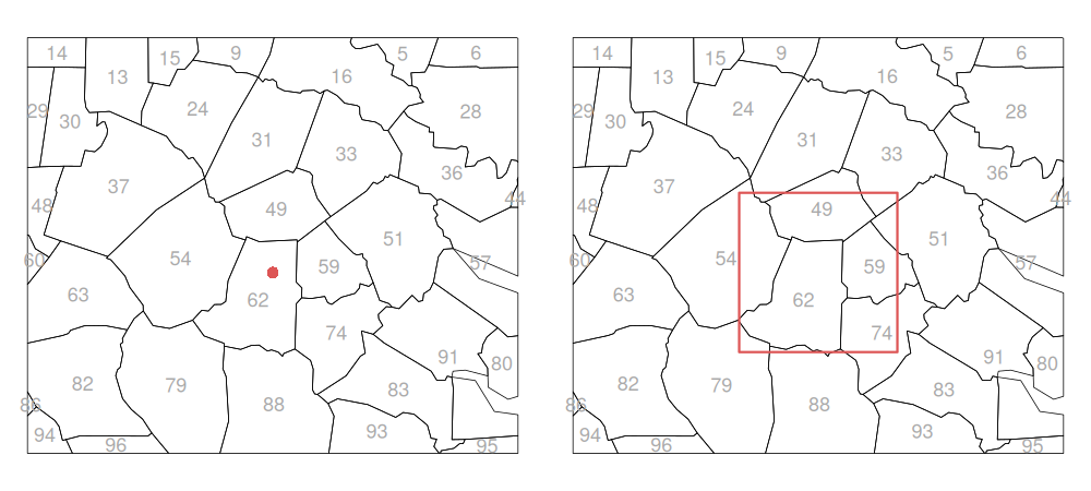
Figure 3: Support of a variable: retrieving the values of the black polygons for the red point or the red square needs knowledge whether values (grey) are associated with each point in a black polygon (point support) or whether they summarise properties of all points in a polygon (block support). Vice versa, going from red to black geometries involves the same problem.

The support of a variable matters when data variables that are associated with non-matching geometries are combined (figure 3). The disaggregation (figure 3 left) or aggregation (figure 3 right) of point support variables is trivial: as all values are known, there is no uncertainty involved. Disaggregation and aggregation of a block support variable is harder: the only thing we can assume is that at a finer (e.g. point) support, the variable will not be constant throughout the geometry. Auxiliary variables are needed to meaningfully model this variation, and obtain downsampled or aggregated values. Examples are downsampling of climate variables [Hewitson and Crane, 1996], or dasymetric mapping of population density [Mennis, 2009].

In addition, when disaggregating (downsampling) or aggregating (upsampling) block support variables, it needs to be known whether sums need to be preserved, as with population counts, or whether averages need to be preserved, as with population density or temperature. When sums need preservation we call the variable extensive, when averages need preservation we call it intensive. These properties may depend on whether considering space or time. As an example, yearly CO₂ emissions of coal power plants have spatial point support (power plant) and temporal block support (years), and are spatially extensive but temporally intensive.

A typical spatial data science analysis starts with reading data from an external source. Ideally, this source should indicate whether variables have point or block support in space and time, and whether they are intensive or extensive. When this is the case, the software used could choose reasonable defaults which methods to use, or raise warnings if unexpected / potentially unsuitable methods would be used. Also, the software in turn could write back the data in a format documenting the support and/or intensive/extensive flag.

Metadata containing support information is often scattered and incomplete. GeoTIFFs can have a metadata flag, AREA_OR_POINT, which, when set, indicates whether raster cells refer to the value of the cell area or at the cell center point. GeoPackage [Yutzler, 2021] or FileGeoDatabase files can have a FieldDomain value that indicates a split policy and a merge policy. These two policies seem to reflect whether a variable is extensive or intensive (table 1).

Redistricting (figure 3 right) always involves both splitting and merging [Do et al., 2015b, a, Goodchild and Lam, 1980, Pebesma and Bivand, 2023]. Table 2 gives examples of extensive and intensive variables for point or block support, associated with point, line or area geometries. Note that while categorical variables can be conceptualised within this framework as (mostly) intensive, their treatment in redistricting will be different. Typically, software such as a Python package Tobler [Knaap et al., 2024] reports proportions per each class in the output.

Variable type	Split policy	Merge policy
extensive	geometry ratio	sum
intensive	duplicate	geometry weighted average

Table 1: Values for the ”split policy” and ”merge policy” field domains for a variable that is spatially extensive or intensive

The NetCDF climate and forecast conventions [Hassell et al., 2017] allow for specifying bounds on dimension variables (space and time) so that particular areas (grid cells) or time periods are made explicit. In addition, it uses the cell_methods attribute for specifying the aggregation method, indicating how a value was aggregated over an area or period (table 3).

Support	Dim	Int/Ext	Example
Point	0	Int	temperature or air quality measured at a sensor
		Ext	power plant CO2 emission, capacity of a wind turbine
	1	Int	Road surface reflectance
		Ext	$\emptyset$ (lines have an infinite number of points)
	2	Int	clay content of the soil
		Ext	$\emptyset$ (areas have an infinite number of points)
Block	0	Int	$\emptyset$ (block support implies non-point geometry)
		Ext	$\emptyset$ (block support implies non-point geometry)
	1	Int	average width of a road, minimum width of a road
		Ext	length of a road, duration to travel a road segment
	2	Int	County average elevation, average temperature, county population density
		Ext	County population total, county area

Table 2: Examples of spatially extensive (Ext) and intensive (Int) variables having Block or Point support, for various geometry dimensions (Dim: 0 for points, 1 for lines, 2 for polygons); $\emptyset$ refers to situations where no examples are possible (reason in italics)

CF encoding	Meaning
pressure:cell_methods = "time: point";	(temporal) point support
ppn:cell_methods = "time: sum";	(temporal) block support, using sum of precipitation
maxtemp:cell_methods = "time: maximum";	indicates (temporal) block support, giving the maximum over the period

Table 3: CF-convention encoding of temporal support, and aggregation method

2.6.1 Point versus block support across languages

R package sf deals to some extent with spatial support: sf data.frames carry an attribute agr (for attribute-geometry relationship) that for each non-geometry variable (”attribute”) is either missing or has one of three values:

constant

: the value has point support, and has constant value for every point of the geometry

aggregate

: the value has block support, and is the result of aggregating some quantity over the geometry

identity

: the value identifies the geometry (e.g., a state name; this is point support)

When operations are carried out on an attribute where point support is assumed (e.g., area-weighted interpolation, or extraction of polygon values a point geometries) and the agr field is missing or aggregate, a warning is raised. Spatial aggregate or summary methods can set the agr flag of the attribute involved to aggregate.

In Python, there is typically no built-in way to carry the information about point and block support or of a type of a variable (intensive vs extensive). The responsibility in this case is left to a user to determine the correct operation for each variable. The same situation is in Julia.

2.7 Data cubes

We use the word ”data cubes” as synonymous with n-dimensional arrays with data values (or tuples) arranged at the combinations of a set of $n\geq 1$ dimension values. In our context, dimensions typically include spatial and/or temporal variables. Dimensions may also be discrete, e.g. a sequence of plant species when the array contains per species abundance values or warehouses’ locations where the array cells contain total sales (c.f. online analytical processing (OLAP) data cubes).

A simple data cube example is a greyscale raster image, which is a two-dimensional array. Multi-band (e.g. Red/Green/Blue) or multi-time images are three-dimensional, while multi-band multi-time images are four-dimensional. Non-raster data cubes can be time series data for a set of (point) sensor locations, or time series with averages for polygon geometries; these are two-dimensional. The case of $n=1$ corresponds to one or more columns in a table.

A lot of large datasets lend themselves well to be represented as data cubes, including Earth observation data, weather forecast or reanalysis data, and climate model forecasts.

Common operations on data cubes include:

• creating regular data cubes from irregular or sparse ones (e.g., image collections collected at different times and having heterogeneous coordinate reference systems, or collections of trajectories),

• interacting with the data cube at a lower spatial and/or temporal resolution, e.g. by pyramids or overviews, where different ways of computing pyramids are possible,

• analysing processes in space, time, or spacetime, e.g. by trend analysis or aggregation, identifying persistent spatial patterns or space-time interactions, and

• creating machine learning models and classifying images.

2.7.1 Data cubes across languages

R packages stars and terra provide two views on representing data cubes, where stars focuses on a generic representation of (raster or vector) n-D cubes, and terra on high performance and scalability for stacks of raster layers (three-dimensional data cubes). Both integrate well with vector data to extract values at points or aggregate data cubes over polygons. Irregular image collections like time series of Sentinel-2 imagery (optionally fetched from a STAC catalog using rstac, Simoes et al. [2021b]), can be transformed into regular four-dimensional data cubes using the gdalcubes package [Appel and Pebesma, 2019], supporting the use of image overviews at lower spatial resolution. A complete workflow from data cube creation to the application of machine learning methods for satellite image time series classification can be achieved using the sits package [Simoes et al., 2021a]. Support for moving features within data cubes is also being conceived in a package under development (post). However, their complex nature still posses challenges for their implementation (see section 2.8).

The Python package xarray is used widely to analyse very large data cubes and is well integrated with dask for parallel processing. xarray provides integration with spatial vector data (like R’s stars and terra) through a series of packages extending its functionality like the package xvec for vector data cubes and zonal statistics. To create data cubes from irregular image collections (with overlapping areas, different CRSes, etc.), StackSTAC takes a STAC catalog and creates a regular data cube as a lazy four-dimensional Dask array. As a coordinating initiative for large-scale geoscientific applications in Python, Pangeo (pangeo.io) provides a community, a software ecosystem, and facilitates the deployment on computing infrastructure.

In Julia, Rasters.jl and YAXArrays.jl can handle arbitrary n-D cubes, building on the shared backends DimensionalData.jl (for spatial indexing) and DiskArrays.jl (for lazy chunk-based operation following Julias’ ‘AbstractArray‘ interface). Rasters.jl also handles stacks of mixed type and n-D layers, that can represent arbitrary NetCDF or grib files, and integrates with all GeoInterface.jl compatible vector data. Cubes can be sampled using points in Rasters.jl, and sampling using lines and polygons can be used with custom ‘Where‘ statements. However, optimised spatial selectors have not yet been implemented. DiskArrayEngine.jl is in early development, but extends DiskArrays.jl for optimised out-of-core chunked operations leveraging Dagger.jl, as an analogue of xarray/dask in the Python ecosystem.

The openEO API [Schramm et al., 2021, Mohr et al., 2025] is a higher level interface to cloud-based processing systems similar to the closed source systems Google Earth Engine [Gorelick et al., 2017] and Sentinel-Hub [Milcinski and Kolaric, 2023]. Clients for openEO in R, Python, Julia, and JavaScript are available, and link to the respective package ecosystems. Examples of openEO-based processing systems are openEO Platform and the Copernicus Data Space Ecosystem.

2.7.2 GIS and modelling community conventions

	GIS	Model (weather, climate, …)
Data types	Vector, raster	Arrays, discrete global grids
Dynamic data	not of primary interest	dominantly present
Height-varying data	ignored	often present (atmosphere)
Coordinates	Cartesian	Geodetic
Raster types	regular	regular, rectilinear or curvilinear
File formats	Esri Shapefile, GeoTIFF	NetCDF, Zarr, GRIB
Data standardisation	Open Geospatial Consortium	NetCDF CDL, CF Conventions
Data support	mostly ignored	CF: bounds, cell methods

Table 4: Comparison of the GIS and modelling communities’ conventions

As opposed to the geospatial ”GIS” community, the geospatial ”modelling” communities comprises for instance weather, climate, oceanographic and geophysical modelling. To a large extent these communities create and share large datasets with predictions, forecasts, or reanalysis results, typically computed as a data cube, i.e. on a regular space and time discretization. For such datacubes the modelling community has largely converged on formats like NetCDF [Rew and Davis, 1990], Zarr [Moore and Kunis, 2023]. The ”climate and forecast” (CF) conventions [Eaton et al., 2003] constrain the very flexible NetCDF format to use specific names for dimensions, units, coordinate reference systems, and to express support and aggregation methods (bounds, cell methods). The data model underlying NetCDF and the CF conventions are also largely used in Zarr data cubes created by these communities. In a number of activities, the geospatial and modelling communities have attempted to find a common ground, these include the definition of geozarr, crs-in-netcdf, the GDAL MultiDimimensional array C++ API, and the existence of NetCDF and Zarr drivers in GDAL. A comparison of differences in conventions between the two communities is given in Table 4.

2.8 Trajectories

While data cubes may cover time series of observations at points locations or for polygons, moving features and their trajectories represent another level of complexity in spatiotemporal data handling and analysis. Acknowledging this fact, the OGC has been working on a new standard – beyond simple features – called moving features [Asahara et al., 2015] which encompasses standardized trajectory encodings in CSV, XML, and JSON, as well as a moving features access standard that specifies functions for movement data (similar to the spatial functions defined in the simple features access standard). In general, the OGC standard supports translation and/or rotation of moving features but not geometry deformation.

One of the main challenges is handling the temporal dimension and how discrete, linear, or step-wise interpolation of geometry and attribute information should be managed. A logical trajectory may consist of separate geometry and attribute time series whose time steps do not necessarily have to align. For example, a vehicle may be fitted with a GPS tracker recording at 1 Hertz and carry a sensor that records events at irregular time intervals. Trajectory data formats should support storage of this data, even if many analysis algorithms require that the data be synced before it can be analyzed further. Another challenge is the visualization of movement data. Common approaches include representing trajectories as directed lines (e.g. using arrow marker, gradients, or tapered lines) or using animation. However, most geospatial visualization libraries have no or very limited support for any of these options.

2.8.1 Trajectories across languages

The review paper of Joo et al. [2020] lists 58 R packages created to deal with moving object or tracking data, with a large focus on movement ecology, and identified 11 packages with good or excellent documentation, mostly based on the CRAN Task View “Handling and Analyzing Spatio-Temporal Data” [Pebesma and Bivand, 2022]. A task view is an overview of R packages for a certain topic. Some of the packages build on each other, however, a large number of packages are isolated even if having similar goals and methods. From this review, the CRAN Task View “Processing and Analysis of Tracking Data” [Joo and Basille, 2023] was created to keep the focus on tracking data. The tracking packages mainly depend on sf, however, there are still a number of dependencies to sp.

There are also numerous open source Python libraries – most of which are based on either Pandas or GeoPandas, including: MovingPandas [Graser, 2019], traffic [Olive, 2019], scikit-mobility [Pappalardo et al., 2021], TransBigData [Yu and Yuan, 2022] trackintel [Martin et al., 2023]. For a full list, see https://github.com/anitagraser/movement-analysis-tools/.

As far as the authors are aware, there are no Julia packages for mobility analysis, although an effort to wrap the MEOS library is currently underway. Implementations discussed in the OGC Moving Features working group include the PostGIS extension MobilityDB [Zimányi et al., 2020] with its core functionality condensed in the C++ library MEOS (Mobility Engine Open Source, a name inspired by GEOS), and a Cesium-based viewer [Kim et al., 2024]. The Moving Features JSON encoding (MF-JSON) is also supported by the Python library MovingPandas.

2.9 Statistical modelling

One purpose common to using spatial data science languages is to fit some statistical model, diagnose it and carry out parameter inferences or create predictions. For doing so, typically data structures are created that specify the input or reflect the outcome of these steps. Inputs are for instance

• a model specification (e.g. an R formula) specifying response, predictors, the type of their relationships, and random effects, or

• a point pattern with its observation window, or

• neighbourhood lists or weights lists specifying which geographic features are related, and to which extent.

Output data structures may include fitted models, e.g. for

• predicting point density from covariates, or

• specifying residual spatial correlation in terms of a covariogram or semivariogram model, or

• spatial error or CAR models, specifying fitted regression coefficients and spatial correlation parameters.

As an example, Bivand [2022] examined R and Python packages for areal data analysis, carrying out the same workflow in both environments and comparing the results. Some data formats used in legacy software, e.g. .GAL files for neighbourhood lists, exist and can help transporting data structures from one environment to the other.

2.10 Cross-language development

A common challenge that all SDSL attendees faced was using software from outside their main language. This is difficult, not only because people tend to specialize on one language at a time, but also because package and environment development systems tend to be language-specific (CRAN does not host Python packages and PyPI does not host R packages, for example). To overcome this challenge, there are two main options: cross-language environment managers and containerisation. The pixi environment manager, first released in June 2023, aims to be a language-agnostic environment manager, with the ability to install R, Julia and spatial packages tested by SDSL attendees.

The current ‘gold standard’ for creating and maintaining cross-language infrastructure — for testing, development, and production — is containerisation. Docker containers can be developed that ‘ship’ with all system dependencies. They can be tagged to specific, immutable versions, providing long-term stability and a near-guarantee of reproducibility [Boettiger and Eddelbuettel, 2017, Nüst and Pebesma, 2021]. Efforts to provide Docker images explicitly for cross-language development are still rare. Numerous projects maintain containers for cross-language spatial data science, including GDS [Arribas-Bel, ], Rocker [Boettiger and Eddelbuettel, 2017, Nüst et al., 2020], geocompx, and b-data.

3 Lessons learned and recommendations

3.1 Lessons learned

The package ecosystems for R, Python and Julia are currently different in a number of respects. The R package sf warns users if they are making implicit assumptions about line or polygon data having point support, and has the ability to label data such that unnecessary warnings are not emitted. It also uses geometrical operations by default on the sphere if coordinates are not projected (geodetic), or warns if it has to use operations in a Cartesian space for geodetic coordinates. It raises errors if operations on objects with different coordinate reference system are carried out, or bring them to a common coordinate reference system as is done when plotted with ggplot2.

Python’s GeoPandas package performs all operations on geodetic coordinates in Cartesian space, while giving the user a warning that values may be wrong and projection is recommended. Developments to use a spherical geometry engine are in progress. There is no tooling that would implicitly help with point and block support or differentiation between intensive and extensive variables, although some PySAL modules ask users to explicitly specify a variable type.

In Julia, most existing geometry interfaces either do not attach metadata such as a coordinate reference system, or have no method to distinguish between the different types of projection. Avoiding combining objects with different coordinate reference systems and applying Cartesian operations to geodetic coordinates is the responsibility of the user, though automatic support for this is improving.

The three different languages have strongly different processes for submitting and sharing packages. R packages distributed on CRAN always need to work with other R packages released, and reverse dependency checks are performed by CRAN on every new submission; changes breaking other packages need to be communicated and clarified in advance.

Python has a complicated mechanism to check whether a release breaks any reverse dependency. Python packages have the ability to require particular versions; package environments can be created to create and maintain collections of packages with particular versions. Furthermore, conda-forge packaging system ensures compatibility of C++ components.

Julia packages follow semantic versioning, and registered packages are required to set compatibility bounds for all declared dependencies. The combination of these factors means it is practically difficult to install packages that are incompatible. Doing reverse dependencies checks, and updating the compatibility bounds are the responsibility of the developer, but much of it is automated - for example, GDAL tests ArchGDAL.jl, GeoDataFrames.jl and Rasters.jl in continuous integration tests. Additionally, the Julia language infrastructure tests the entire ecosystem against all new release candidates to ensure breakages do not occur in relation to changes in the language itself.

3.2 Recommendations

3.2.1 Open standards

It is encouraging to see that involvement in the development of open geospatial is no longer restricted to members of the Open Geospatial Consortium (OGC), and takes place in issues of public OGC GitHub repositories (for instance for GeoZarr and GeoParquet), or even completely outside OGC communication channels (e.g. STAC, GDAL, and openEO). OGC recently increased its individual and academic membership fee from 550 USD to 2500 USD per year, making it more and more of a business activity. Requiring more than one open source implementation is still not a requirement for a standard to be adopted by OGC.

It would be convenient to have routines to verify polygons form a coverage (i.e. are not overlapping), or to create non-overlapping polygons from overlapping ones, in a way that all spatial data science languages can profit from. A prototypical implementation is found in R package sf, with n-ary intersection and difference, and in Python package geoplanar [Rey et al., 2023] providing a tooling to fix common planarity issues.

The increased diversity in data frame libraries, increased diversity in geospatial tooling, and increasing data size have highlighted a need for connectivity that extends beyond the columnar memory model implemented separately in each of the spatial data science languages. Wider adoption of GeoParquet as a more efficient file format for whole-file read/write and wider adoption of GeoArrow as a common metadata standard and memory model may help address these challenges.

3.2.2 Field domains

Splitting spatially extensive block support variables to point geometries should at all times be avoided: one would need an infinite number of zero valued points that should sum to the polygon sum. With discrete computers this cannot be realised, and software should warn against attempts doing so. Intensive and extensive variables should both refer to quantitative variables, otherwise sums, proportions and averages do not make sense. Split rules can only apply to variables with non-point geometries.

As table 1 reveals, split and merge policies follow from a variable being spatially extensive or intensive, and hence one of them is obsolete. The question remains what to do when a data source has two contradictory values set, e.g. split policy ”duplicate” and merge policy ”sum”. A less ambiguous approach would be to have a single field domain called is_spatially_extensive with a boolean value.

3.2.3 Geodetic coordinates, spherical geometry

For a consistent handling of simple feature geometries on a spherical geometry, one has to augment the simple feature standard in the following way:

• in addition to the POLYGON EMPTY one needs the POLYGON FULL to define the polygon formed by the entire surface of the sphere. In addition to this WKT definition one would need a WKB representation of this; the value used for this by the S2Geometry library, WKB of POLYGON ((0 -90, 0 -90)) would be a pragmatic choice. R package sf now supports the POLYGON FULL.

• straight lines on the sphere are not straight: the obvious choice is to use shortest arcs over the sphere (”great circle distance”). When importing GeoJSON files, one may need to add nodes to longer line segments on plate carrée, to follow the GeoJSON definition of a straight line.

• one needs to define winding order of polygon rings, e.g. the way S2Geometry does this: the area left of the lines when connecting nodes in order of appearance is the inside. When importing polygons, a pragmatic default, also taken by BigQuery GIS [Mozumder and Karthikeya, 2022] is to define the inner side of a ring as the smaller of the two areas, but full user control is needed to work e.g. with the polygon of the oceans.

3.2.4 Community management

R, being the oldest of the spatial data science languages, has now finished a full development circle where crucial infrastructure packages (rgdal and rgeos) have been developed, used, maintained, and retired. Retirement involved a process taking more than two years, informing all reverse dependencies when this would be coming and how they could adapt to use modern alternatives.

The Python community is trying to coordinate the development efforts potentially refactor core packages to support current needs to avoid the need for retirement (which is also not entirely possible due to the design of Python packaging systems) and migration. The clear example is the recent merge of the PyGEOS project into Shapely, resulting in Shapely 2.0 release with completely revised interface to GEOS.

Julia is much earlier in the cycle, and while it has the benefit of learning from the work of the R and Python ecosystems, has a relatively small developer community, largely focused on high-performance or big-data modelling applications.

The developer communities would benefit from a stronger diversity, and one way to increase that is to create a welcoming culture for newcomers, for comments, to adopt good code of conducts, and to follow the experience collected in organisations like rOpenSci and pyOpenSci. Several efforts towards this goal have already started as precursors and within the SDSL community. To foster support, guidance and to increase interaction between community members, discord channels are available both for the geocompx project and the SDSL community . The geocompx discord is a open forum to seek support, ask questions, and showcase exciting work. The SDSL discord serves as a tool to foster discussions, both among developers and users on spatial data science concepts, methods, packages and programming languages.

3.2.5 Cross-language collaboration and infrastructure

Communities and infrastructure for cross-language collaboration are in their infancy. However, an increasing number of projects are using multiple languages for spatial data science for research, testing and deployment of services in production. This creates a need for more cross-language events like the SDSL initiative that formed a basis for this paper.

One of the findings from the SDSL sessions is that cross-language infrastructure is in its infancy. Projects such as ‘Rocker’ and ‘Pixi’, mentioned in Section 2.10, have made a start in this direction, but they are still focussed on one language with support for other languages being add-ons, rather than core features. We recommend that more work is done to provide both the technical infrastructure and social environments for constructive cross-language work for spatial data science developers, users and educators.

The geocompx project is “a community-driven effort to provide resources for learning and teaching about geocomputation in multiple programming languages”. Three books on the topic of geocomputation, one focusing on R [Lovelace et al., 2025], one on Python [Dorman et al., 2025], one on Julia, are available online through this project. The Spatial Data Science book [Pebesma and Bivand, 2023] is also fully available online, a second edition is evolving with subtitle “With applications in R and Python”, and contains tabbed code sections with R and Python tabs. The Quarto publishing system can be used to create books or websites from notebook-style markdown documents that contains multiple data science languages. Jupyter [Kluyver et al., 2016] notebooks can also handle multiple languages, but not in single document, as Quarto does.

3.2.6 Future events

The general impression of the attendees of the workshops on Spatial Data Science Languages was very positive, as many developers and users usually work in relative isolation, with asynchronous on-line communication. It was agreed to repeat this event, and to combine it then with a hackathon in order to do practical work, including testing, comparison, and further interoperability experiments. Not all aspects of spatial data science have been considered yet and future events should also address other relevant domains such as spatial network analysis, web-mapping and visualization, among others.

References

- Anselin et al. [2006] L. Anselin, I. Syabri, and Y. Kho. Geoda : An introduction to spatial data analysis. Geographical Analysis, 38(1):5–22, 2006. doi: https://doi.org/10.1111/j.0016-7363.2005.00671.x. URL https://onlinelibrary.wiley.com/doi/abs/10.1111/j.0016-7363.2005.00671.x.
- Appel and Pebesma [2019] M. Appel and E. Pebesma. On-demand processing of data cubes from satellite image collections with the gdalcubes library. Data, 4(3), 2019. URL https://www.mdpi.com/2306-5729/4/3/92.
- [3] D. Arribas-Bel. gds_env: A containerised platform for geographic data science. URL https://darribas.org/gds_env.
- Asahara et al. [2015] A. Asahara, R. Shibasaki, N. Ishimaru, and D. Burggraf. Ogc® moving features encoding part i: Xml core. Open Geospatial Consortium Inc, 2015. URL https://portal.opengeospatial.org/files/14-083r2.
- Becker et al. [1986] R. A. Becker, J. M. Chambers, and A. R. Wilks. The new S Language: A programming environment for data analysis and graphics. Pacific Grove, CA: Wadsworth & Brooks/Cole, 1986.
- Bezanson et al. [2017] J. Bezanson, A. Edelman, S. Karpinski, and V. B. Shah. Julia: A fresh approach to numerical computing. SIAM review, 59(1):65–98, 2017.
- Bivand [2022] R. Bivand. R packages for analyzing spatial data: A comparative case study with areal data. Geographical Analysis, 54(3):488–518, 2022. doi: https://doi.org/10.1111/gean.12319. URL https://onlinelibrary.wiley.com/doi/abs/10.1111/gean.12319.
- Bivand et al. [2013] R. Bivand, E. Pebesma, and V. Gómez-Rubio. Applied spatial data analysis with R, Second edition. Springer, NY, 2013. URL http://www.asdar-book.org/.
- Bivand et al. [2017] R. Bivand, T. Keitt, and B. Rowlingson. rgdal: Bindings for the ’Geospatial’ Data Abstraction Library, 2017. URL https://CRAN.R-project.org/package=rgdal. R package version 1.2-15.
- Bloch [2024] M. Bloch. mapshaper, 2024. URL https://github.com/mbloch/mapshaper.
- Boettiger and Eddelbuettel [2017] C. Boettiger and D. Eddelbuettel. An Introduction to Rocker: Docker Containers for R. The R Journal, 9(2):527, 2017. ISSN 2073-4859. doi: 10.32614/RJ-2017-065.
- Butler and Gillies [2005] H. Butler and S. Gillies. Open source python gis hacks. Open Source Geospatial, 5, 2005.
- Butler et al. [2016] H. Butler, M. Daly, A. Doyl, S. Gillies, S. Hagen, and T. Schaub. The geojson format, 2016. ISSN 2070-1721. URL https://tools.ietf.org/html/rfc7946.
- Butler et al. [2023] H. Butler, S. Gillies, A. Stewart, B. Pedersen, and M. W. Taves. rtree, Oct. 2023. URL https://github.com/Toblerity/rtree.
- Chrisman [2012] N. Chrisman. A deflationary approach to fundamental principles in GIScience. In Francis Harvey (ed.) Are there fundamental principles in Geographic Information Science?, pages 42–64. CreateSpace, United States, 2012.
- conda-forge community [2015] conda-forge community. The conda-forge Project: Community-based Software Distribution Built on the conda Package Format and Ecosystem, July 2015. URL https://doi.org/10.5281/zenodo.4774216.
- Dem et al. [2025] J. L. Dem, R. Blue, F. Driesprong, N. Li, A. Pitrou, G. Szadovszky, G. Wu, A. Mokashi, A. Levenson, N. Kollár, ggershinsky, nkollar, J. Chen, J. Apple, dvryaboy, C. Lian, C. Aniszczyk, emkornfield, zivanfi, G. Pang, A. Lamb, E. Seidl, L. Volker, T. Deng, mwish, T. Armstrong, d becker, V. Ganesh, and D. Z. Chen. apache/parquet-format, 2 2025. URL https://github.com/apache/parquet-format.
- den Bossche et al. [2023] J. V. den Bossche, K. Jordahl, M. Fleischmann, J. McBride, J. Wasserman, M. Richards, A. G. Badaracco, A. D. Snow, J. Tratner, J. Gerard, B. Ward, M. Perry, C. Farmer, G. A. Hjelle, M. Taves, E. ter Hoeven, M. Cochran, rraymondgh, S. Gillies, G. Caria, L. Culbertson, R. Bell, M. Bartos, N. Eubank, sangarshanan, J. Flavin, S. Rey, J. Gardiner, maxalbert, and A. Bilogur. geopandas/geopandas: v0.14.0, Sept. 2023.
- Do et al. [2015a] V. H. Do, C. Thomas-Agnan, and A. Vanhems. Spatial reallocation of areal data: a review. Rev. Econ. Rég. Urbaine, 1/2:27–58, 2015a. URL https://www.tse-fr.eu/sites/default/files/medias/doc/wp/mad/wp_tse_397_v2.pdf.
- Do et al. [2015b] V. H. Do, C. Thomas-Agnan, and A. Vanhems. Accuracy of areal interpolation methods for count data. Spatial Statistics, 14:412 – 438, 2015b. ISSN 2211-6753. doi: 10.1016/j.spasta.2015.07.005.
- Dorman et al. [2025] M. Dorman, A. Graser, J. Nowosad, and R. Lovelace. Geocomputation with Python. CRC Press, 2025. ISBN 9781032460659.
- Dunnington et al. [2024] D. Dunnington, K. Barron, J. Van den Bossche, M. Visser, B. Teuscher, B. Ward, C. Korner, M. Dobias, N. Crane, and R. Li. geoarrow/geoarrow, 2024. URL https://github.com/geoarrow/geoarrow.
- Eaton et al. [2003] B. Eaton, J. Gregory, B. Drach, K. Taylor, S. Hankin, J. Caron, R. Signell, P. Bentley, G. Rappa, H. Höck, et al. Netcdf climate and forecast (cf) metadata conventions. URL: http://cfconventions. org/Data/cf-conventions/cf-conventions-1.8/cf-conventions. pdf, 2003.
- Eddelbuettel [2013] D. Eddelbuettel. Seamless R and C++ integration with Rcpp. Springer, 2013.
- Gillies et al. [2023a] S. Gillies, R. Buffat, J. Arnott, M. W. Taves, K. Wurster, A. D. Snow, M. Cochran, E. Sales de Andrade, and M. Perry. Fiona, Oct. 2023a. URL https://github.com/Toblerity/Fiona.
- Gillies et al. [2023b] S. Gillies, C. van der Wel, J. Van den Bossche, M. W. Taves, J. Arnott, B. C. Ward, and others. Shapely, Oct. 2023b. URL https://github.com/shapely/shapely.
- Gillies et al. [2013–] S. Gillies et al. Rasterio: geospatial raster i/o for Python programmers, 2013–. URL https://github.com/rasterio/rasterio.
- Goodchild and Lam [1980] M. F. Goodchild and N. S. N. Lam. Areal interpolation: a variant of the traditional spatial problem. Department of Geography, University of Western Ontario London, ON, Canada, 1980.
- Gorelick et al. [2017] N. Gorelick, M. Hancher, M. Dixon, S. Ilyushchenko, D. Thau, and R. Moore. Google earth engine: Planetary-scale geospatial analysis for everyone. Remote Sensing of Environment, 202:18–27, 2017. ISSN 0034-4257. doi: https://doi.org/10.1016/j.rse.2017.06.031. URL https://www.sciencedirect.com/science/article/pii/S0034425717302900. Big Remotely Sensed Data: tools, applications and experiences.
- Graser [2019] A. Graser. Movingpandas: efficient structures for movement data in python. GIForum, 1:54–68, 2019.
- GRASS Development Team [2024] GRASS Development Team. Geographic Resources Analysis Support System (GRASS GIS) Software, Version 8.4. Open Source Geospatial Foundation, USA, 2024. URL https://grass.osgeo.org.
- Harris et al. [2020] C. R. Harris, K. J. Millman, S. J. van der Walt, R. Gommers, P. Virtanen, D. Cournapeau, E. Wieser, J. Taylor, S. Berg, N. J. Smith, R. Kern, M. Picus, S. Hoyer, M. H. van Kerkwijk, M. Brett, A. Haldane, J. F. del Río, M. Wiebe, P. Peterson, P. Gérard-Marchant, K. Sheppard, T. Reddy, W. Weckesser, H. Abbasi, C. Gohlke, and T. E. Oliphant. Array programming with NumPy. Nature, 585(7825):357–362, Sept. 2020. doi: 10.1038/s41586-020-2649-2. URL https://doi.org/10.1038/s41586-020-2649-2.
- Hassell et al. [2017] D. Hassell, J. Gregory, J. Blower, B. N. Lawrence, and K. E. Taylor. A data model of the climate and forecast metadata conventions (cf-1.6) with a software implementation (cf-python v2. 1). Geoscientific Model Development, 10(12):4619–4646, 2017.
- Herring [2011] J. Herring. Opengis implementation standard for geographic information-simple feature access-part 1: Common architecture. Open Geospatial Consortium Inc, page 111, 2011. URL http://portal.opengeospatial.org/files/?artifact_id=25355.
- Hewitson and Crane [1996] B. C. Hewitson and R. G. Crane. Climate downscaling: techniques and application. Climate Research, 7(2):85–95, 1996.
- Holmes et al. [2024] C. Holmes, J. Van den Bossche, T. Schaub, K. Barron, M. Mohr, ghobona, E. Rouault, A. Asuero, J. A. Torrens, felixpalmer, X. Nogueira, M. Barry, M. Pronk, L. Yee, J. Aponte, J. Brockmeier, J. Yu, J. de la Torre, J. Wasserman, D. Dunnington, C. Benavent, B. Hulette, and B. Ward. opengeospatial/geoparquet, 2024. URL https://github.com/opengeospatial/geoparquet.
- Hoyer and Hamman [2017] S. Hoyer and J. Hamman. xarray: N-D labeled arrays and datasets in Python. Journal of Open Research Software, 5(1), 2017. doi: 10.5334/jors.148. URL https://doi.org/10.5334/jors.148.
- Hughes-Noehrer et al. [2024] L. Hughes-Noehrer, N. Aubert Bonn, M. De Maria, T. R. Evans, E. K. Farran, L. Fortunato, E. L. Henderson, N. Jacobs, M. R. Munafò, S. L. K. Stewart, and A. J. Stewart. UK Reproducibility Network open and transparent research practices survey dataset. Scientific Data, 11(1):912, Aug. 2024. ISSN 2052-4463. doi: 10.1038/s41597-024-03786-z.
- Joo and Basille [2023] R. Joo and M. Basille. CRAN Task View: Processing and Analysis of Tracking Data, 2023. URL https://CRAN.R-project.org/view=Tracking. Version 2023-03-07.
- Joo et al. [2020] R. Joo, M. E. Boone, T. A. Clay, S. C. Patrick, S. Clusella-Trullas, and M. Basille. Navigating through the r packages for movement. Journal of Animal Ecology, 89(1):248–267, 2020. doi: https://doi.org/10.1111/1365-2656.13116. URL https://besjournals.onlinelibrary.wiley.com/doi/abs/10.1111/1365-2656.13116.
- Kim et al. [2024] D. Kim, WijaeCho, H. Jeong, H.-G. Ryoo, T. Kim, and B. Hards. aistairc/mf-cesium, 2024. URL https://github.com/aistairc/mf-cesium.
- Kluyver et al. [2016] T. Kluyver, B. Ragan-Kelley, F. Pérez, B. Granger, M. Bussonnier, J. Frederic, K. Kelley, J. Hamrick, J. Grout, S. Corlay, et al. Jupyter notebooks–a publishing format for reproducible computational workflows. In Positioning and power in academic publishing: Players, agents and agendas, pages 87–90. IOS press, 2016.
- Knaap et al. [2024] E. Knaap, R. X. Cortes, S. Rey, M. Fleischmann, D. Arribas-Bel, J. Gaboardi, J. Parry, and P. Frontiera. pysal/tobler: v0.12.0, Nov. 2024. URL https://doi.org/10.5281/zenodo.14031618.
- Lovelace et al. [2025] R. Lovelace, J. Nowosad, and J. Muenchow. Geocomputation with R. CRC Press, second edition, 2025. ISBN 9781032248882.
- Martin et al. [2023] H. Martin, Y. Hong, N. Wiedemann, D. Bucher, and M. Raubal. Trackintel: An open-source python library for human mobility analysis. Computers, Environment and Urban Systems, 101:101938, 2023. ISSN 0198-9715. doi: https://doi.org/10.1016/j.compenvurbsys.2023.101938. URL https://www.sciencedirect.com/science/article/pii/S0198971523000017.
- Mennis [2009] J. Mennis. Dasymetric mapping for estimating population in small areas. Geography Compass, 3(2):727–745, 2009.
- Milcinski and Kolaric [2023] G. Milcinski and P. Kolaric. Sentinel hub-federated on-demand ard generation. In EGU General Assembly Conference Abstracts, pages EGU–4160, 2023.
- Mohr et al. [2025] M. Mohr, E. Pebesma, J. Dries, S. Lippens, B. Janssen, D. Thiex, G. Milcinski, B. Schumacher, C. Briese, M. Claus, A. Jacob, P. Sacramento, and P. Griffiths. Federated and reusable processing of earth observation data. Scientific Data, 12, 2025. URL https://doi.org/10.1038/s41597-025-04513-y.
- Moore and Kunis [2023] J. Moore and S. Kunis. Zarr: A cloud-optimized storage for interactive access of large arrays. In Proceedings of the Conference on Research Data Infrastructure, volume 1, 2023.
- Mozumder and Karthikeya [2022] C. Mozumder and N. S. Karthikeya. Geospatial Big Earth Data and Urban Data Analytics, pages 57–76. Springer International Publishing, Cham, 2022. ISBN 978-3-031-14096-9. doi: 10.1007/978-3-031-14096-9˙4. URL https://doi.org/10.1007/978-3-031-14096-9_4.
- Nüst et al. [2020] D. Nüst, D. Eddelbuettel, D. Bennett, R. Cannoodt, D. Clark, G. Daróczi, M. Edmondson, C. Fay, E. Hughes, L. Kjeldgaard, et al. The rockerverse: packages and applications for containerization with r. arXiv preprint arXiv:2001.10641, 2020. URL https://arxiv.org/abs/2001.10641.
- Nüst and Pebesma [2021] D. Nüst and E. Pebesma. Practical reproducibility in geography and geosciences. Annals of the American Association of Geographers, 111(5):1300–1310, 2021. doi: 10.1080/24694452.2020.1806028. URL https://doi.org/10.1080/24694452.2020.1806028.
- Olive [2019] X. Olive. traffic, a toolbox for processing and analysing air traffic data. Journal of Open Source Software, 4(39):1518, 2019. doi: 10.21105/joss.01518. URL https://doi.org/10.21105/joss.01518.
- Pappalardo et al. [2021] L. Pappalardo, F. Simini, G. Barlacchi, and R. Pellungrini. Scikit-mobility: a python library for the analysis, generation and risk assessment of mobility data, 2021.
- Pebesma [2018] E. Pebesma. Simple Features for R: Standardized Support for Spatial Vector Data. The R Journal, 10(1):439–446, 2018. doi: 10.32614/RJ-2018-009. URL https://doi.org/10.32614/RJ-2018-009.
- Pebesma and Bivand [2005] E. Pebesma and R. Bivand. Classes and methods for spatial data in R. R News, 5(2):9–13, November 2005. URL https://CRAN.R-project.org/doc/Rnews/.
- Pebesma and Bivand [2022] E. Pebesma and R. Bivand. CRAN Task View: Handling and Analyzing Spatio-Temporal Data, 2022. URL https://CRAN.R-project.org/view=SpatioTemporal. Version 2022-10-01.
- Pebesma and Bivand [2023] E. Pebesma and R. Bivand. Spatial Data Science: With Applications in R. Chapman and Hall/CRC, 2023. doi: 10.1201/9780429459016. URL https://doi.org/10.1201/9780429459016.
- R Core Team [2023] R Core Team. R: A Language and Environment for Statistical Computing. R Foundation for Statistical Computing, Vienna, Austria, 2023. URL https://www.R-project.org/.
- [60] M. Raasveldt and H. Muehleisen. DuckDB. URL https://github.com/duckdb/duckdb.
- Rew and Davis [1990] R. Rew and G. Davis. Netcdf: an interface for scientific data access. IEEE computer graphics and applications, 10(4):76–82, 1990.
- Rey et al. [2023] S. Rey, N. Wajiha, and M. Fleischmann. geoplanar, Oct. 2023. URL https://github.com/sjsrey/geoplanar.
- Rey and Anselin [2007] S. J. Rey and L. Anselin. Pysal: A python library of spatial analytical methods. The Review of Regional Studies, 37(1):5–27, 2007.
- Rey and Janikas [2006] S. J. Rey and M. V. Janikas. Stars: Space–time analysis of regional systems. Geographical Analysis, 38(1):67–86, 2006. doi: https://doi.org/10.1111/j.0016-7363.2005.00675.x. URL https://onlinelibrary.wiley.com/doi/abs/10.1111/j.0016-7363.2005.00675.x.
- Schramm et al. [2021] M. Schramm, E. Pebesma, M. Milenković, L. Foresta, J. Dries, A. Jacob, W. Wagner, M. Mohr, M. Neteler, M. Kadunc, T. Miksa, P. Kempeneers, J. Verbesselt, B. Gößwein, C. Navacchi, S. Lippens, and J. Reiche. The openeo api–harmonising the use of earth observation cloud services using virtual data cube functionalities. Remote Sensing, 13(6), 2021. ISSN 2072-4292. doi: 10.3390/rs13061125. URL https://www.mdpi.com/2072-4292/13/6/1125.
- Simoes et al. [2021a] R. Simoes, G. Camara, G. Queiroz, F. Souza, P. Andrade, L. Santos, A. Carvalho, and K. Ferreira. Satellite image time series analysis for big earth observation data. Remote Sensing, 13(13):2428, 2021a. doi: 10.3390/rs13132428.
- Simoes et al. [2021b] R. Simoes, F. Souza, M. Zaglia, G. R. Queiroz, R. Santos, and K. Ferreira. Rstac: An r package to access spatiotemporal asset catalog satellite imagery. In 2021 IEEE International Geoscience and Remote Sensing Symposium IGARSS, pages 7674–7677, 2021b. doi: 10.1109/IGARSS47720.2021.9553518.
- Snow et al. [2023] A. D. Snow, J. Whitaker, and M. Cochran. pyproj, Oct. 2023. URL https://github.com/pyproj4/pyproj.
- Team [2023] R. D. Team. RAPIDS: Libraries for End to End GPU Data Science, 2023. URL https://rapids.ai.
- Van Rossum et al. [2007] G. Van Rossum et al. Python programming language. In USENIX annual technical conference, volume 41, pages 1–36. Santa Clara, CA, 2007.
- Vink et al. [2025] R. Vink, S. de Gooijer, A. Beedie, M. E. Gorelli, nameexhaustion, O. Peters, G. Burghoorn, W. Guo, J. van Zundert, G. Hulselmans, C. Grinstead, Marshall, chielP, I. Turner-Trauring, L. Mitchell, L. Manley, M. Santamaria, D. Heres, H. Harbeck, J. Magarick, K. Genockey, ibENPC, deanm0000, I. Koutsouris, M. Wilksch, eitsupi, J. Leitao, M. van Gelderen, and R. G. Serrão. pola-rs/polars: Python polars 1.19.0, Jan. 2025. URL https://doi.org/10.5281/zenodo.14597402.
- Wickham et al. [2019] H. Wickham, M. Averick, J. Bryan, W. Chang, L. D. McGowan, R. François, G. Grolemund, A. Hayes, L. Henry, J. Hester, et al. Welcome to the tidyverse. Journal of Open Source Software, 4(43):1686, 2019. URL https://joss.theoj.org/papers/10.21105/joss.01686.
- Yu and Yuan [2022] Q. Yu and J. Yuan. Transbigdata: A python package for transportation spatio-temporal big data processing, analysis and visualization. Journal of Open Source Software, 7(71):4021, 2022. doi: 10.21105/joss.04021. URL https://doi.org/10.21105/joss.04021.
- Yutzler [2021] J. Yutzler. OGC® GeoPackage encoding standard. 2021. URL https://www.geopackage.org/spec131/index.html.
- Zimányi et al. [2020] E. Zimányi, M. Sakr, and A. Lesuisse. MobilityDB: A mobility database based on PostgreSQL and PostGIS. ACM Trans. Database Syst., 45(4), Dec. 2020. doi: 10.1145/3406534.