NuiScene: Exploring Efficient Generation of Unbounded Outdoor Scenes

Abstract

In this paper, we explore the task of generating expansive outdoor scenes, ranging from castles to high-rises. Unlike indoor scene generation, which has been a primary focus of prior work, outdoor scene generation presents unique challenges, including wide variations in scene heights and the need for a method capable of rapidly producing large landscapes. To address this, we propose an efficient approach that encodes scene chunks as uniform vector sets, offering better compression and performance than the spatially structured latents used in prior methods. Furthermore, we train an explicit outpainting model for unbounded generation, which improves coherence compared to prior resampling-based inpainting schemes while also speeding up generation by eliminating extra diffusion steps. To facilitate this task, we curate NuiScene43, a small but high-quality set of scenes, preprocessed for joint training. Notably, when trained on scenes of varying styles, our model can blend different environments, such as rural houses and city skyscrapers, within the same scene, highlighting the potential of our curation process to leverage heterogeneous scenes for joint training.

Figure 1: Our model enables efficient, unbounded generation of large outdoor scene geometry. Scenes are textured with SceneTex [6].

Figure 2: A scene generated by our model, trained on multiple scenes. We texture the scene using SceneTex. As shown, our model combines elements from different scenes in the dataset such as castles and skyscrapers. For the untextured mesh, please see the supplement (Figure˜16).

1 Introduction

Large-scale outdoor scene generation is crucial for many applications such as enabling immersive world-building for open-world video games, cinematic CGI environments, and VR simulations. Traditionally, crafting these vast outdoor environments required extensive manual labor and significant resources. Fortunately, recent advances in AI-driven content generation techniques offer the potential to significantly enhance accessibility and efficiency for this task.

Following the trend of diffusion models in image generation—such as Stable Diffusion [36]—generative models for creating standalone 3D objects [45, 23] are also rapidly maturing. The success of such models is partly driven by large-scale datasets like Objaverse [9]. However, large-scale scene generation remains limited, with many works focused on indoor environments [17, 44, 32, 4]. While some methods utilize semantic car datasets [25, 30, 26] or CAD models [29], these datasets lack high-quality geometry and have limited scene variation and height. Compared to previous methods, we tackle a challenging task with three key challenges: 1) enabling fast and efficient generation of outdoor scenes with varying height distributions, 2) generating scenes with varying styles into a cohesive and continuous scene, 3) curating a dataset that facilitates exploration into such methods and supports joint training of heterogeneous scenes.

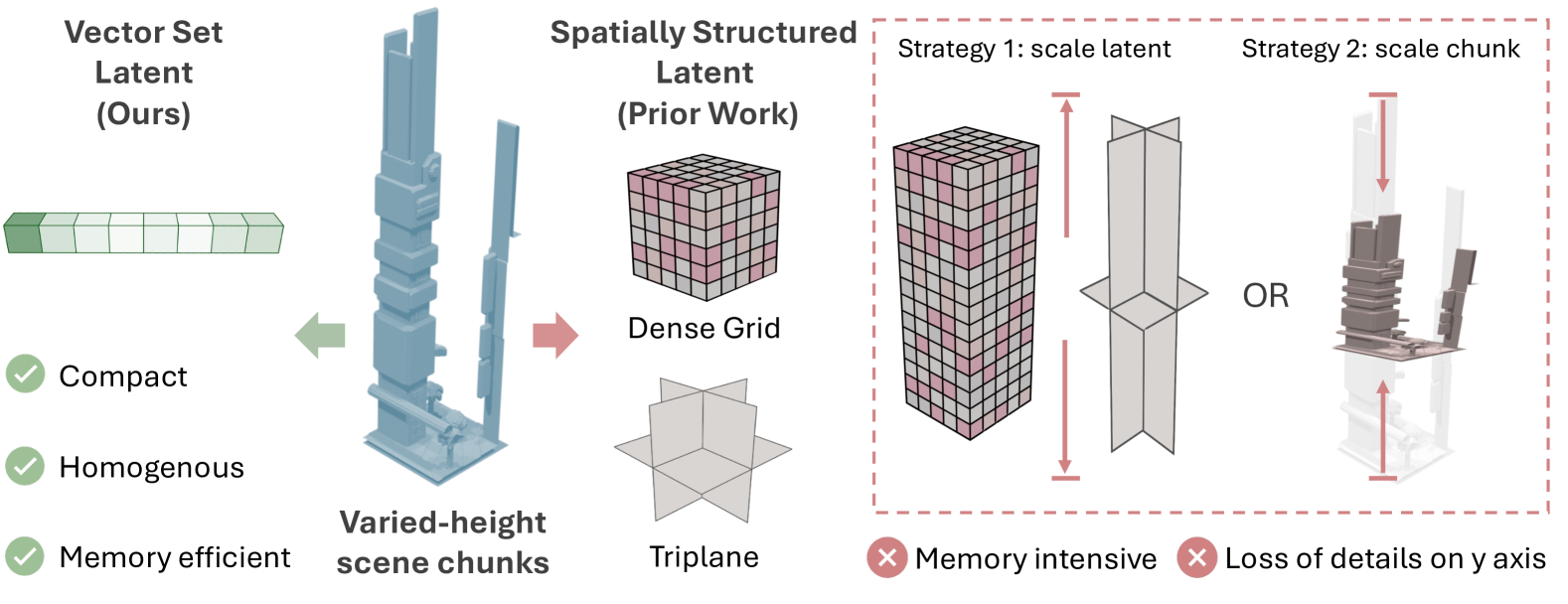
Figure 3: To accommodate scene chunks of varying heights, vector sets offer a compact and uniform representation, whereas prior work relies on spatially structured latents that require scaling either the latent resolution or the chunk itself for compatibility, resulting in high memory usage or loss of detail.

Previous works on generating unbounded indoor scenes using 3D-Front [11] assume scenes can be divided into equal-sized cubes, and learn spatially structured latents like triplanes [44] or dense feature grids [32] for compression. This approach struggles with outdoor scenes featuring buildings like skyscrapers with significantly different heights. As shown in Figure˜3, naively scaling these representations can result in intensive memory usage. Rescaling the scene via normalization will also degrade details. To address this, we compress scene chunks into vector sets using 3DShape2VecSet [49], achieving better compression than triplanes for more efficient training and higher quality generations. Additionally, we train our diffusion model for explicit outpainting, further improving inference speed over methods [44, 32] utilizing resampling-based inpainting like RePaint [31] which requires additional diffusion steps. Furthermore, prior methods focus on uniform datasets, such as indoor or urban driving scenes. In contrast, we aim to explore generative models that can bring together scenes with different context such as castles and cities. We showcase our model’s ability to generate scenes with distinct styles in Figure˜2.

Another key limitation for such a task is the lack of openly available high quality outdoor scenes for training, making developing such methods more challenging. 3D-Front [11] is used by many prior works to train unbounded indoor scene generation. However, it lacks variation in scene height and non-furniture geometry. Semantic driving datasets [42, 2] and urban reconstructions [35, 13, 12] lack high quality geometry compared to artist-created meshes. Objaverse [9] includes many scenes that could facilitate training for this task. However, several challenges remain. Notably, these meshes lack a unified global scale, and feature highly varied ground geometries—ranging from very thick to thin planes—making it difficult to train a generative model effectively as a homogeneous dataset. To address this, we curate a small set of scenes from Objaverse. We clean ground geometries and establish a unified scale, enabling the development of methods that handle (1) diverse scene height distributions and (2) outdoor geometry from varied sources and styles. We show that this data process pipeline is effective in enabling the joint training of heterogeneous scenes in a unified generative model.

In summary, NuiScene provides the following contributions: Efficient Representation. We propose using vector sets to encode chunks of varying sizes into a uniform representation, enhancing both training efficiency and scene generation quality. Outpainting Model. Unlike previous methods relying on slow resampling-based outpainting, we train our diffusion model to explicitly outpaint by conditioning on previously generated whole chunks, leading to faster inference time generation. Cross Scene Generation. We demonstrate that our efficient NuiScene model, trained on four curated scenes, can blend scenes of different styles (e.g., medieval, city), highlighting both the model’s capability and effectiveness of our curation process. NuiScene43. A dataset of 43 moderate to large sized scenes from Objaverse, with cleaned ground geometries and unified scales. This enables joint training on heterogeneous scenes, supporting the development of methods for unbounded scene generation with 1) diverse scene heights, and 2) various styles.

2 Related Work

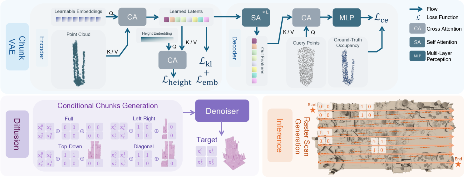
Figure 4: Overview of our VAE and diffusion models. For the VAE we use vector sets [49] for latent compression. For the diffusion model we train a conditional outpainting model with four different settings to allow for fast generation in a raster scan pattern during inference.

3D Scene Gen with T2I Priors. Recently, methods leveraging priors from text-to-image (T2I) diffusion models [36] and monocular depth estimation methods [3, 22, 19] have gained popularity for generating 3D scenes from text or images [8, 38, 48, 10]. These approaches use T2I models to generate RGB images and depth prediction models to extract geometric information, which is then used to distill or optimize 3D geometry. This enables continuous outpainting and unbounded scene generation by shifting the camera and synthesizing new regions. While the strong priors of T2I models allow for open-domain scene generation, accumulated errors in depth predictions lead to geometric distortions and limitations in long-range consistency.

3D Bounded Single Exemplar Scene Gen. Several works focus on generating 3D scenes from a single exemplar [41, 18, 43, 27], follow a coarse-to-fine progressive approach by capturing patch statistics across scales. Similar to SinGAN [37], SinGRAV [41], 3INGAN [18], and Wu and Zheng [43] adopt a pyramid of GANs, where discriminators operate on smaller patch sizes to enforce local consistency while allowing diverse global compositions. Li et al. [27] introduces EM-like optimization for patch matching and blending across different scales. Although these methods generate scenes with varying compositions and aspect ratios, they are limited to bounded generation, and producing an entire scene at once leads to increasing memory costs for larger scenes.

3D Unbounded Scene Gen. One common method for 3D unbounded scene generation start by dividing scenes into smaller chunks and using an autoencoder to compress them into latents, such as triplane or dense grids. A diffusion model is then trained on the scene chunk latents. By overlapping the current chunk with previously generated ones, these methods enable continuous outpainting relying on resampling-based inpainting methods like RePaint [31] requiring additional diffusion steps.

Unbounded outdoor scene generation has been explored using synthetic and real-world semantic driving datasets like CarlaSC [42] and SemanticKITTI [2]. While these datasets enable relatively large-scale scene generation, they lack high-quality geometry. SemCity [26] follows the approach outline above and uses triplanes as the latent representation. PDD [30] employs a pyramid discrete diffusion model on raw semantic grids directly with a scene subdivision module that conditions generation on overlapping regions. Unlike PDD which conditions on overlapping regions using dense grids, our approach conditions on entire neighboring chunks with richer context. These methods suffer from limited geometric quality, and height variation due to the dataset.

There are also other methods that take different approaches to unbounded outdoor generation. CityDreamer [46] and InfiniCity [29] leverage top-down views for unbounded generation but are limited to cityscapes with low-resolution geometry. SceneDreamer [7] and Persistent Nature [5] are promising directions to generate unbounded 3D worlds from only 2D images. However, without explicit 3D supervision, the resulting geometry lacks detail.

For unbounded indoor scene generation, methods typically train on 3D-Front [11] and assume cubic scene chunks. BlockFusion [44], like SemCity, compresses scene chunks into triplanes. It then employs another VAE to further compress the triplanes into a lower resolution, reducing redundancy in the representation to improve diffusion learning. LT3SD [32] encodes TUDF chunks into multi-level dense feature grid latent trees, organizing both its autoencoder and diffusion models in a hierarchical manner for coarse-to-fine chunk generation. While these representations perform well for indoor scenes with fixed ceiling heights, they struggle to scale to outdoor environments with significant height variations, as shown in Figure˜3. To tackle this, we use a vector set representation which compresses chunks into a uniform size, offering better compression and performance. And enable faster generation with a outpainting model.

3 Method

We represent a large outdoor scene as a collection of local scene chunks, where a VAE learns to compress individual chunks into vector sets, and a diffusion model generates neighboring chunks in a $2\times 2$ grid using the VAE’s learned representation. By combining both models, we enable continuous chunk generation, supporting unbounded outdoor scene synthesis. Our overall training framework follows the Latent Diffusion Model (LDM)[36], with an illustration provided in Figure˜4.

The dataset curation process is outlined in Sec.˜3.1, followed by how training chunks are sampled. To explore efficient large-scale scene generation, we experiment with triplane and vector set latents. The VAE backbone and the process of querying points from these representations to obtain occupancies are described in Sec.˜3.2. For fast inference without relying on resampling-based inpainting methods, we train an explicit outpainting diffusion model, detailed in Sec.˜3.3. Optionally, textures can be generated using SceneTex [6]. More details are available in the supplement (S2.3).

3.1 Dataset

Filtering and Preprocessing. We begin by filtering Objaverse [9] using multi-view embeddings from DuoduoCLIP [24] to select 43 high-quality scenes. Next, we establish a consistent scale by labeling scenes with relative scales. We then convert each scene into an occupancy grid with a resolution multiplied by its labeled relative scale and generate meshes using the marching cubes algorithm for point cloud sampling. To ensure uniform ground geometry across scenes, we ensure a uniform thickness below the ground level for each scene. For more details on the dataset curation process, please refer to the supplement (S1).

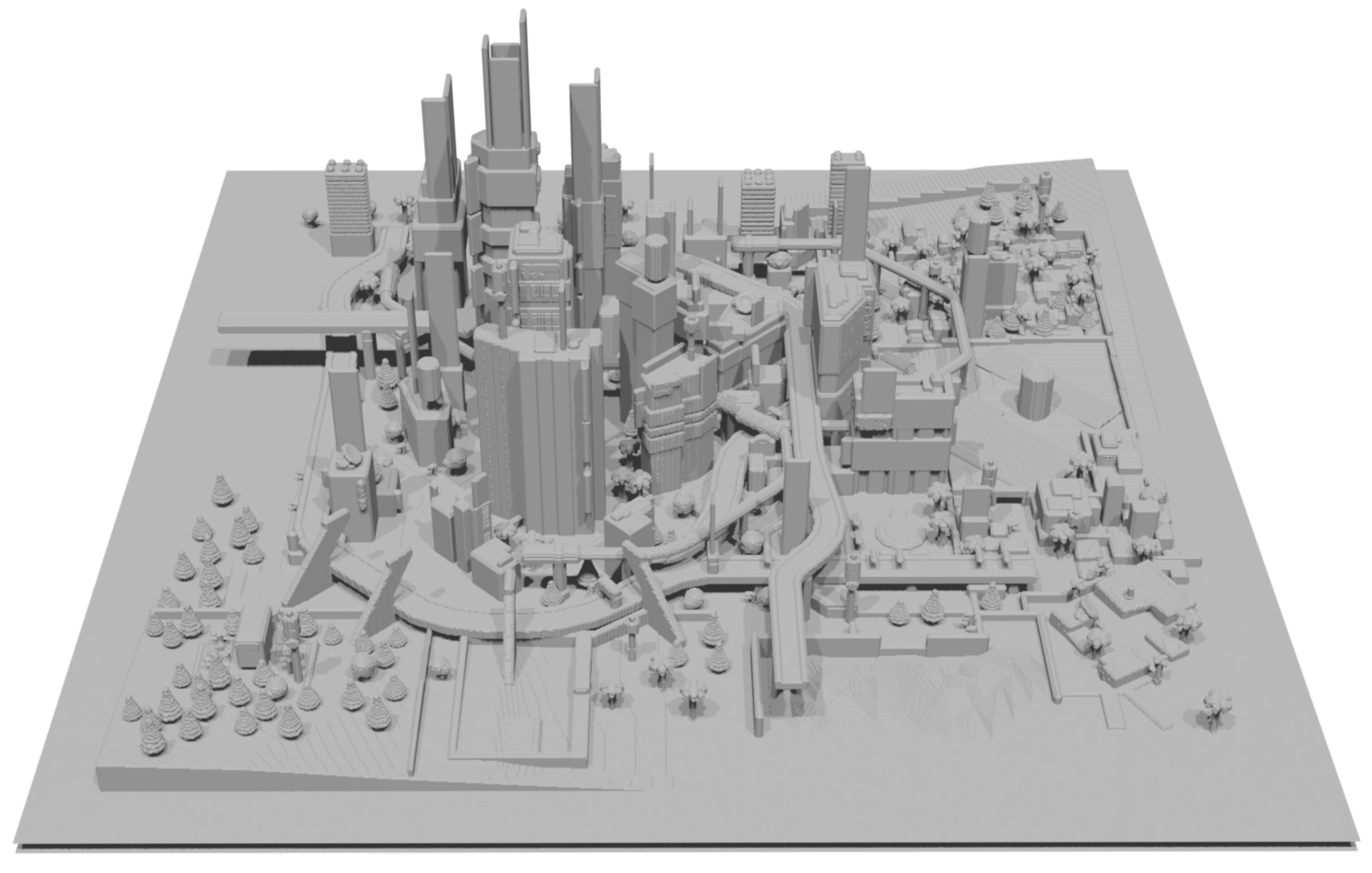
Figure 5: A sample scene processed using our curation pipeline. The occupancy is processed with marching cubes to get the mesh.

Chunk Sampling. A sample scene processed through our curation pipeline is shown in Figure˜5. The resulting occupancy grid has dimensions of occ$\in\{0,1\}^{1059\times 478\times 1059}$. To facilitate training, we divide the scene into smaller chunks of size $(50,h_{\text{vox}},50)$ along the $x,y,z$ axis, where $y$ represents the height axis. Chunks are sampled via occ[i-25:i+25,:,k-25:k+25], where $i$ and $k$ are sample coordinates along the $x$ and $z$ axis of the scene, respectively. The height of the sampled chunk $h_{\text{vox}}\leq 478$ is determined by the tallest occupied voxel within each chunk. As a result, chunk heights vary.

For training, we sample coordinates within the chunk’s occupancy grid as $\bm{r}_{\text{vox}}=(x_{\text{vox}},y_{\text{vox}},z_{\text{vox}})$, where $0\leq x_{\text{vox}},z_{\text{vox}}\leq 50$ and $0\leq y_{\text{vox}}\leq h_{\text{vox}}$ along with the corresponding occupancy $\tilde{o}$ at each coordinate. The sampled coordinates are then normalized as: $\bm{r}=2*(\bm{r}_{\text{vox}}/\bm{d})-1$, where $\bm{d}=(d_{x},d_{y},d_{z})$ is the normalization scale for each axis. The ground truth height of the chunk is computed as $\tilde{h}=2*(h_{\text{vox}}/50)-1$. The chunk’s point cloud is also normalized using the same procedure with $\bm{d}=(50,50,50)$.

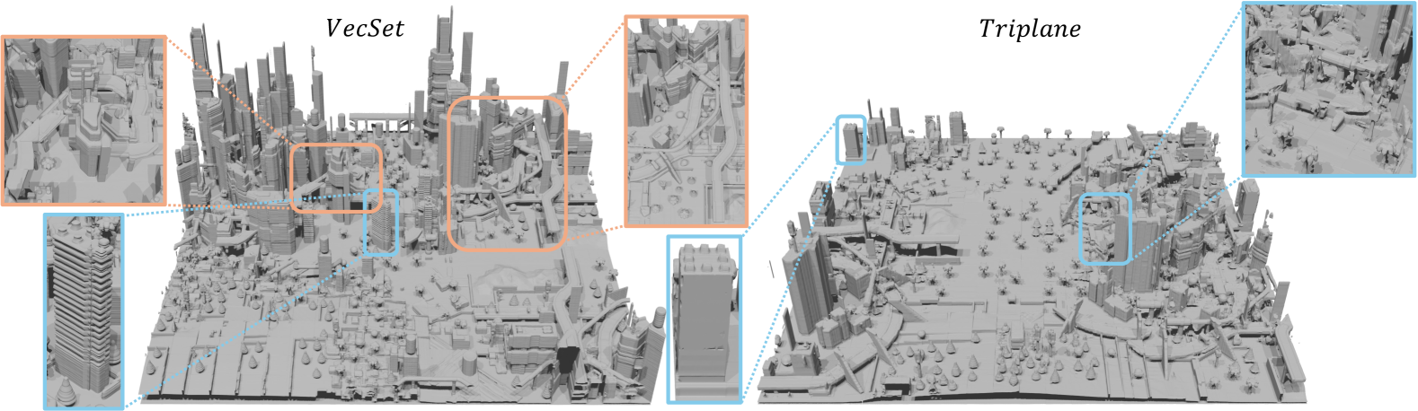
Figure 6: We show generation results for the vector set and triplane baseline trained on a single scene. Orange boxes and zoomed-in renders highlight chunk outpainting coherence, while blue boxes illustrate scene geometry (zoom in for details). Zoomed-in renders may also have adjusted camera angles for clarity. The triplane model struggles with building details and introduces noisy artifacts, whereas the vector set model has better fidelity. While models can generate continuous chunks with smoothly connected roads and pipes (orange box, right), they sometimes fail to maintain coherence across chunks, leading to broken bridges (orange box, left).

3.2 Chunk VAE

3.2.1 Encoder

Our encoder $\mathcal{E}$ compresses sampled scene chunks $P$, which consists of varying heights into a uniform set of vectors. For each chunk $P_{i}$, we uniformly sample a fixed size point cloud $\bm{p}\in\mathbb{R}^{N_{p}\times 3}$ of $N_{p}$ points. Following 3DShape2Vecset [49], we use a cross-attention (CA) layer to aggregate the point clouds into a compact representation, leveraging a learnable set of fixed features with a reduced number of tokens. Next, a fully connected (FC) layer predicts the mean and variance, from which we apply the reparameterization trick [20] to generate embeddings for the chunks. This results in $\bm{z}^{\bm{p}}=\mathcal{E}(\bm{p})\in\mathbb{R}^{V\times c}$, where $V$ is the number of vectors and $c$ is the channel size.

However, we found that this is prone to posterior collapse [39], a common issue in VAEs. To address this, we introduce an alternative regularization strategy. Specifically, we sample another point cloud $\bm{q}\in\mathbb{R}^{N_{p}\times 3}$ from the same chunk $P_{i}$ and enforce consistency between their embeddings: $\mathcal{L}_{\text{emb}}=(\bm{z}^{\bm{p}}-\bm{z}^{\bm{q}})^{2}$. This prevents VAE collapse as it prevents the encoder from ignoring its input and enforces similar embeddings for point clouds sampled from the same chunk, while adding only a minimal overhead—just an additional pass through the CA and fully connected layers.

Furthermore, we predict the chunk’s height from its embedding to prune unnecessary occupancy predictions at inference time. Since the embedding may be generated by the diffusion model, we do not have access to the ground truth height of each chunk during inference. To account for this, we learn a height embedding $\bm{e}_{h}\in\mathbb{R}^{1\times c}$ and use it to query the latent representation, yielding the predicted height $\hat{h}=\text{FC}(\text{CA}(\bm{z^{p}},\bm{e}_{h}))$. The height loss is calculated as $\mathcal{L}_{\text{height}}=(\hat{h}-\tilde{h})^{2}$ where $\tilde{h}$ is the ground truth height.

3.2.2 Decoder

Next, we pass the embedding through $L$ self-attention (SA) layers in the decoder to obtain the output features $\bm{f}_{\text{out}}=\text{SA}^{(L)}\circ...\circ\text{SA}^{(1)}(\bm{z^{p}})$, which are then passed to either the vector set or triplane head to decode the occupancy.

Triplane. For the triplane head, $\bm{f}_{\text{out}}$ is reshaped into a triplane and upsampled using deconvolution layers, similar to LRM [15], yielding a feature grid $T\in\mathbb{R}^{3\times h_{\text{tri}}\times w_{\text{tri}}\times c_{\text{tri}}}$. Query points $\bm{r_{tri}}$ as outlined in Sec.˜3.1 are normalized with $\bm{d}=(50,50*S,50)$, where the scale factor $S$ further compresses points along the y-axis. To ensure all coordinates remain within $[-1,1]$ for valid triplane sampling, we apply clamping. Note that we define $-1$ as the left or bottom bound of the triplane and $1$ as the right or top bound. Features are extracted via bilinear interpolation from the triplanes, concatenated, and processed by a fully connected layer to predict occupancies $\hat{o}_{r}$.

Vector Set. The query point $\bm{r_{vec}}$ is calculated with a normalizing scale of: $\bm{d}=(50,50,50)$. Occupancy is predicted via cross-attention: $\hat{o}_{r}=\text{FC}(\text{CA}(\bm{f}_{\text{out}},\text{PE}(\bm{r_{vec}})))$, where PE is the fourier embedding of the query points.

Loss. We supervise the occupancy with binary cross entropy $\mathcal{L}_{\text{ce}}=\text{BCE}(\hat{o}_{r},\tilde{o}_{r})$ with the ground truth occupancy $\tilde{o}_{r}$. The embedding is supervised with a KL loss $\mathcal{L}_{\text{kl}}$. See Zhang et al. [49] for more details. The total loss is $\mathcal{L}=\lambda_{\text{kl}}\mathcal{L}_{\text{kl}}+\lambda_{\text{emb}}\mathcal{L}_{\text{emb}}+\lambda_{\text{ce}}\mathcal{L}_{\text{ce}}+\lambda_{\text{height}}\mathcal{L}_{\text{height}}$, and $\lambda$s are the loss weights. We note that, unlike the triplane method, the vector set allows query points to have ranges beyond $[-1,1]$. This is because cross-attention and positional encoding can directly handle arbitrary values without requiring them to be within a specific range for valid sampling, unlike spatial latent-based approaches like triplanes.

Inference Time Decoding. During inference, since we have no access to the encoding point cloud or ground truth height $\tilde{h}$, we use the predicted height $\hat{h}$ to prune unnecessary calculations. First, our model predicts $\hat{h}$. Then, we generate all query coordinates $\bm{r}_{\text{vox}}$ within a volume of shape $(50,50*(\hat{h}+1)/2,50)$, where each query point $\bm{r}$ is normalized via $2*(\bm{r}_{\text{vox}}/\bm{d})-1$. These normalized coordinates query the latent representation for occupancy predictions, and we apply marching cubes to the occupancy volume to reconstruct the chunk’s mesh.

3.3 Diffusion

Unlike existing models [26, 44, 32] that utilize RePaint [31] for outpainting, which requires extra diffusion steps, we propose a more efficient approach. Our outpainting diffusion model generates four chunks at once in a $2\times 2$ grid, conditioning on previously generated chunks using different patterns to handle all scenarios as shown in Figure˜4 for continuous generation in a raster scan order.

We adopt DDPM [14] for diffusion probabilistic modeling. For diffusion training, we sample a quadrant of neighboring chunk latents $\{\bm{z}^{0},\bm{z}^{1},\bm{z}^{2},\bm{z}^{3}\}$ arranged in a $2\times 2$ grid sampled from the scene and encoded by the VAE. The order of chunks can be seen in Figure˜4. At each training step we sample a Gaussian noise $\bm{\epsilon}\sim\mathcal{N}(0,\mathbf{I})$ at a randomly sampled timestep $t\in[1,T]$ which is added to the quadrant of embeddings to obtain noisy latents $\bm{X}_{t}=\{\bm{x}^{0}_{t},\bm{x}^{1}_{t},\bm{x}^{2}_{t},\bm{x}^{3}_{t}\}\in\mathbb{R}^{4\times V\times c}$, where $\bm{x}^{i}_{t}\in\mathbb{R}^{V\times c}$ is the noised $i$-th latent at timestep $t$.

Our diffusion model takes noisy latents $\bm{X}_{t}$ as input, along with a binary mask indicating existing chunks and corresponding conditional embeddings providing context for outpainting. We consider four possible conditioning configurations, each with a corresponding mask $M$ and condition embeddings $Z_{\text{cond}}$, as illustrated in Figure˜4. The mask is defined as $M=\{\bm{m}^{0},\bm{m}^{1},\bm{m}^{2},\bm{m}^{3}\}\in\mathbb{R}^{4\times V\times 1}$, where $M$ has four possible values: $\{\mathbf{0},\mathbf{0},\mathbf{0},\mathbf{0}\}$, $\{\mathbf{1},\mathbf{0},\mathbf{1},\mathbf{0}\}$, $\{\mathbf{1},\mathbf{1},\mathbf{0},\mathbf{0}\}$ or $\{\mathbf{1},\mathbf{1},\mathbf{1},\mathbf{0}\}$, with $\mathbf{0},\mathbf{1}\in\mathbb{R}^{V\times 1}$. The condition embeddings are constructed based on the corresponding masks $\{\mathbf{0},\mathbf{0},\mathbf{0},\mathbf{0}\}$, $\{\bm{z}^{0},\mathbf{0},\bm{z}^{2},\mathbf{0}\}$, $\{\bm{z}^{0},\bm{z}^{1},\mathbf{0},\mathbf{0}\}$ and $\{\bm{z}^{0},\bm{z}^{1},\bm{z}^{2},\mathbf{0}\}$ with $\mathbf{0}\in\mathbb{R}^{V\times c}$ to form $Z_{\text{cond}}$. The mask, conditional embeddings and positional embeddings PE are concatenated to obtain the condition of the diffusion model:

$$\bm{C}=M\oplus Z_{\text{cond}}\oplus\text{PE}$$ (1)

We use a UNet-style Transformer from Craftsman [28] as the backbone for denoising network $\epsilon_{\theta}$. The model is then trained to denoise latents via:

$$\mathbb{E}_{\bm{X},\bm{C},\bm{\epsilon}\sim\mathcal{N}(0,\mathbf{I}),t}\left[\|\bm{\epsilon}-\epsilon_{\theta}((\bm{X}_{t}\oplus\bm{C}),t)\|^{2}_{2}\right]$$ (2)

Note that during diffusion model training, one of the four configurations is randomly selected, along with the corresponding mask and conditional embeddings. Please see the supplemental (Algorithm˜1) for more details on how the raster scan generation works during inference.

4 Experiment

4.1 Dataset

For single-scene experiments, we use the processed scene from Figure˜5 and follow the chunk sampling process outlined in Sec.˜3.1 for VAE training. Instead of sampling individual chunks, we sample larger quad-chunks of size $(100,h_{vox},100)$, which consists of a 2x2 grid of smaller chunks $(50,h_{vox},50)$. Sampling is done along the $x$ and $z$ axes using occ[i-50:i+50,:,k-50:k+50]. We sample 100k quad-chunks in total, with 95k used for training and 5k for validation. While these chunks may overlap, they are not identical, as they come from different $x$ and $z$ coordinates. We define the batch size as the number of quad-chunks used for training, with the quad-chunks divided into 4 smaller chunks during VAE training. For the diffusion model, the quad-chunks’ point clouds are encoded using the VAE for diffusion training with the 4 different patterns.

For multi-scene experiments, we add three additional scenes in additional to the single scene for training. In total we sample 300k quad-chunks from these scenes. Please see the supplement (Figure˜10) for more visualizations.

4.2 Evaluation Metrics

Reconstruction For reconstruction metrics, we report Chamfer Distance (CD), F-Score, and IoU following Zhang et al. [49] by comparing ground truth and reconstructed chunks on the validation set. CD and F-Score are computed from 50k sampled points per chunk using a threshold of $2/50$, the voxel length of our sampled chunks. For IoU, we sample 20k occupancy values, with 5k from occupied regions and 5k from unoccupied regions, along with 10k near-surface points along the chunk’s surface.

Generation We evaluate the generation quality of our diffusion models using Fréchet PointNet++ [34] Distance (FPD) and Kernel PointNet++ Distance (KPD), following Zhang et al. [49]. We use the Pointnet++ model from Point-E [33] following Yan et al. [47]. Specifically, we sample 10k quad-chunks from the diffusion model, compute their surface point clouds (2048 points), and compare them to 10k sampled quad-chunks from the original scene.

Table 1: Comparison of VAE training resources for vector set vs triplane backbones. Training for all experiments was run on 2 L40S GPUs, total batch size and memory across 2 gpus are reported. The # Latents is the size of the latent for the VAE backbone and Output Res indicates the triplane size after deconvolution. Increasing the output triplane resolution to $3\times 128^{2}$ causes the model to exceed memory limits (OOM).

Method	BS	# Latents	Output Res	S	Time (hr)	Mem. (GB)
triplane	40	$3\times 4^{2}$	$3\times 32^{2}$	6	35.9	35.7
	40	$3\times 4^{2}$	$3\times 64^{2}$	6	58.5	55.7
	40	$3\times 4^{2}$	$3\times 128^{2}$	6	-	OOM
vecset	40	16	-	-	36.1	36.6

Table 2: Comparison of difffusion training resources of vector set representation against triplanes. Training across all experiments was run on 1 A6000 GPU. The # Tokens are the token length for the transformer.

Method	BS	# Tokens	Time (hr)	Mem. (GB)
triplane	192	$4\times 3\times 4^{2}$	27.6	24.4
vecset	192	$4\times 16$	11.1	10.4

4.3 Model and Baselines

We use triplane representations as a baseline for this task, given their widespread use in prior work [26, 44]. We do not directly adopt BlockFusion’s triplane architecture, as it requires fitting triplanes for all dataset chunks, a process that took thousands of GPU hours on 3D-Front. Instead, we implement a VAE backbone with architecture similar to LRM[15] discussed in Sec.˜3.2.

We exclude dense grid methods [30, 32] due to their high memory demands, which scale cubically with resolution, compared to the quadratic growth of triplanes. In our task, the height can be up to about 8.5 times greater than the $x$ and $z$ dimensions for scene chunks in Figure˜5, further exacerbating memory usage. Additionally, LT3SD [32] requires multi-scale training for both the autoencoder and diffusion models, increasing training time.

VAE For triplane baselines, we explore configurations with $V=3\times 4\times 4$, varying the number of deconvolution layers, which affects output resolution, and the normalization scale $S$ (see Tab.˜2). For the vector set model, compressing to $V=16$ preserves geometric fidelity while enabling efficient diffusion training. Both representations use a channel size of $c=64$, and a sampled point cloud size of $N_{p}=4096$. We set the output triplane channel $c_{tri}=40$. The decoder has $L=24$ self-attention layers, and all models are trained for $160$ epochs. Each training iteration samples $4096$ query points per chunk for occupancy supervision.

Diffusion For all models, we use a 25-layer UNet-like transformer [28] for diffusion. The triplane diffusion model operates on embeddings from the VAE with the output triplane resolution of $h_{tri}=w_{tri}=64$ and $S=6$. We train all models for $320$ epochs and a batch size of $192$. The transformer processes tokens of length $4\times V$ as the diffusion model generates a 2x2 grid of chunks at once.

4.4 Single Scene

In single-scene experiments, we demonstrate the effectiveness of representing scene chunks as vector sets compared to spatially structured latents like triplanes. VAE reconstruction results (Sec.˜4.4.1) and diffusion model comparisons (Sec.˜4.4.2) show that the vector set representation achieves better compression, leading to improved training efficiency and superior performance over triplanes.

4.4.1 VAE Reconstruction

Tab.˜3 presents the quantitative reconstruction results, showing that the vector set model outperforms all triplane settings. We also report whether occupancy queries are pruned using the predicted height $\hat{h}$ or the ground truth height $\tilde{h}$ when computing meshes for CD and F-Score. The similar values in both cases indicate the accuracy of our height prediction.

The triplane models are constrained by the VAE’s output resolution, with performance improving as resolution increases from $3\times 32^{2}$ to $3\times 64^{2}$. However, for tall scenes, coordinate clamping during triplane sampling prevents reconstruction of tall buildings exceeding the scaling factor of $S=6$. Increasing $S$ to $8.5$ (matching the tallest chunk) severely degrades performance due to precision loss from excessive compression along the y-axis. While further increasing resolution to $128^{2}$ via deconvolution is possible, it results in out-of-memory (OOM) on two L40S GPUs ( Tab.˜2). In contrast, the vector set model provides better compression ($V=16$ vs $V=3\times 4\times 4$) while requiring similar training time and memory as the lowest-resolution triplane model, demonstrating its efficiency in representing scene chunks and superior performance.

Table 3: Quantitative comparison of reconstruction across different VAE backbones. Here $\hat{h}$ indicates that the predicted height was used for the occupancy prediction and $\tilde{h}$ the ground truth height.

Method	Output Res/S	IOU$\uparrow$	CD $(\hat{h})\downarrow$	F-Score $(\hat{h})\uparrow$	CD $(\tilde{h})\downarrow$	F-Score $(\tilde{h})\uparrow$
triplane	$3\times 32^{2}$/$6$	0.734	0.168	0.508	0.168	0.508
	$3\times 64^{2}$/$8.5$	0.805	0.105	0.705	0.105	0.705
	$3\times 64^{2}$/$6$	0.940	0.064	0.831	0.064	0.831
vecset	-	$\mathbf{0.989}$	$\mathbf{0.055}$	$\mathbf{0.864}$	$\mathbf{0.055}$	$\mathbf{0.863}$

4.4.2 Diffusion

Table 4: Comparison of triplane and vecset diffusion models for generated quad-chunks. KPD scores are multiplied $10^{3}$.

Method	FPD$\downarrow$	KPD$\downarrow$
triplane	1.406	2.589
vecset	$\mathbf{0.571}$	$\mathbf{0.951}$

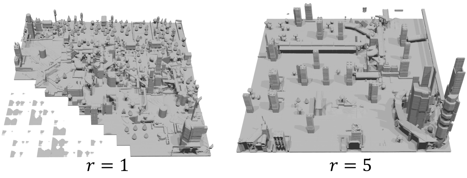
Figure 7: We compare generation results using RePaint [31] for outpainting for resampling steps $r=1$ and $r=5$.

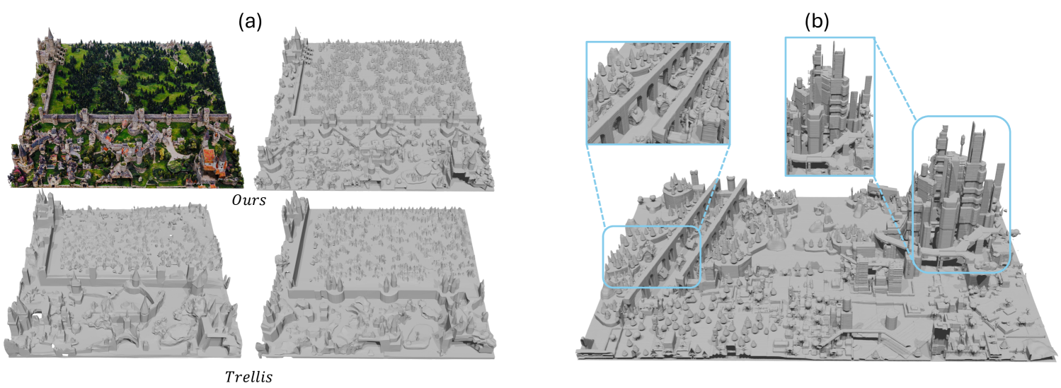
Figure 8: We present results from our NuiScene model trained on multiple scenes. In Figure (a), the top-right shows the generated geometry, while the top-left displays the textured model using SceneTex [6]. We render these models and feed them into Trellis [45] for reconstruction (zoom in to see details). It can be seen that our method showcases better geometric detail. Figure (b) presents a large scene generated by our model, showcasing its ability to blend elements from different scenes in the dataset.

Quality. The FPD and KPD scores (Tab.˜4) show that the vector set diffusion model outperforms the baseline triplane diffusion model as well. Qualitative results for a 21x21 chunk scene (Figure˜6) demonstrate the vector set model’s ability to generate finer details, especially for buildings, whereas the triplane model struggles with details and introduces noisy artifacts which contributes to the higher FPD and KPD scores, likely due to compression of query points along the y axis. Additionally, as shown in Tab.˜2, the vector set model trains about 2.5 times faster and uses half the VRAM, benefiting from three times fewer tokens with a smaller $V$.

Table 5: We benchmark generation time on 1 RTX 2080Ti for generating $21\times 21$ chunks using RePaint with 5 resampling steps and our explicit outpainting method with the vecset diffusion model, and also report the triplane diffusion model’s generation time.

Method	Outpaint	Scene Size	Emb Gen Time (s)	Occ Decode Time (s)
vecset	RePaint	$21\times 21$	1030.54	60.74
triplane	explicit	$21\times 21$	219.42	30.21
vecset	explicit	$21\times 21$	217.79	76.59

Outpainting. We compare against the inpainting method RePaint [31], widely used in prior works [44, 32, 26] for unbounded outpainting. To ensure a fair comparison, we generate scenes in the same order and with the same overlaps as our outpainting model. However, in RePaint, the mask and conditional embeddings are set to zero, with existing chunk conditions incorporated through its iterative re-sampling process. RePaint results for resampling steps $r=1$ and $r=5$ are shown in Figure˜7. Without resampling ($r=1$), inter-chunk connections lack coherence, and the process sometimes collapses into broken chunks, likely due to the model repeatedly conditioning on noisy diffusion-generated chunks. With $r=5$, coherence improves, but the RePaint baseline still produces less diverse scenes and occasional collapses, even with more resampling steps (Figure˜14, supplement). Additionally, iterative re-sampling is significantly slower than our outpainting method (Tab.˜5), as inference time scales with the number of resampling steps, whereas our method does not require resampling.

Our outpainting method is not perfect, and some chunks may still be poorly connected or discontinuous. In Figure˜6, the right orange box shows coherently connected chunks for our vector set diffusion model, while the left-side orange box highlights issues such as misaligned bridges or non-continuous chunks with visible gaps and seams. We believe that this is largely due to the limited dataset size, where certain objects may not appear often enough, leading to insufficient training examples for seamless generation.

4.5 Multiple Scenes

In Sec.˜4.4, we demonstrated the advantages of vector sets over triplanes for efficient representation, allowing flexible handling of scene chunks with varying heights. As well as the effectiveness of our outpainting model for fast large scale outdoor scene generation. However, training on a single scene leads to overfitting, with sub-scenes resembling the training data, despite the model’s ability to generate some novel compositions ( Figure˜13, supplement). To assess its generalization ability and validate our curation process for NuiScene43, we extend training to three additional scenes using the vector set backbone.

Figure˜8 (b) shows a scene generated by our model, with blue boxes highlighting how it integrates elements (rural houses, aqueduct, skyscraper) from two distinct scenes. This demonstrates its generalization ability, as such combinations are absent from the training data. Our model’s efficient generation process, combined with a curation process that unifies diverse scenes into a cohesive training dataset, enables the seamless stitching of chunks from disjoint environments.

We further compare our approach with Trellis [45], a state-of-the-art image-to-3D object generation method, using its official HuggingFace demo. The top right of Figure˜8 (a) shows the geometry produced by our model, with the top left displaying a textured version using SceneTex. We render both textured and geometry-only meshes and use them as inputs for Trellis, with results shown at the bottom. As seen, Trellis produces coarser geometric details, as its single latent representation for entire scenes limits fine details in large environments. In contrast, our model represents each chunk separately, enabling higher-detail and unbounded scene generation. This highlights a key limitation of current object generation methods, which struggle to scale effectively for unbounded scene generation.

5 Conclusion

Limitations One limitation of our model is the limited number of training scenes, as we currently pre-sample chunks offline, leading to high storage costs when sampling a large amount of chunks from scenes. More efficient scene representations, such as octrees, could enable online sampling and support training on the entire NuiScene43 dataset. Another limitation is the lack of control in our generative model, as we currently lack text descriptions or attributes for individual chunks, making controllable conditional generation difficult. However, we may be able to leverage foundation models [21, 1] to allow for semantic map or text conditioning. A related challenge, also present in previous works [44, 32, 26, 30], is the lack of global context and larger control. The model only conditions on a small portion of chunks for generation, making it difficult to make large-scale decisions, such as city planning with roads.

We introduce NuiScene, a method for expansive outdoor scene generation across heterogeneous scenes. Our approach addresses key challenges posed in this task, such as large height variations between scene chunks, by representing them as vector sets. This allows for efficient training and flexible querying, overcoming the limitations of prior works that rely on spatially structured latents. Another crucial aspect of large-scale outdoor generation is speed. Instead of slow inpainting methods like RePaint, we train an outpainting model that enables fast inference without resampling steps while ensuring better coherence between chunks. To support this task, we curate a high-quality dataset from moderate to large scenes, enabling the exploration of (1) varied scene heights and (2) heterogeneous scene blending. Trained on multiple scenes, our model showcases cross-scene generation by seamlessly merging distinct elements that never co-occurred in the training data, creating a cohesive scene and validating the effectiveness of our curation pipeline. We believe further automation of this process will expand available datasets, unlocking open-domain large-scale scene generation.

Acknowledgements. This work was funded by a CIFAR AI Chair, an NSERC Discovery grant, and a CFI/BCKDF JELF grant. We thank Jiayi Liu, and Xingguang Yan for helpful suggestions on improving the paper.

Supplementary Material

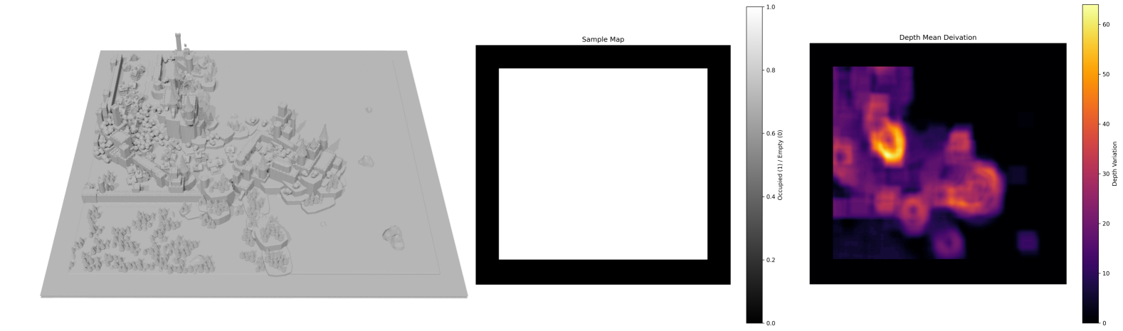
Figure 9: Sample and depth mean deviation maps are calculated for sampling chunks from scenes. The sample map is a binary map defining valid x and z coordinates where quad chunks are fully occupied. And the depth mean variation map is used to filter out overly flat regions.

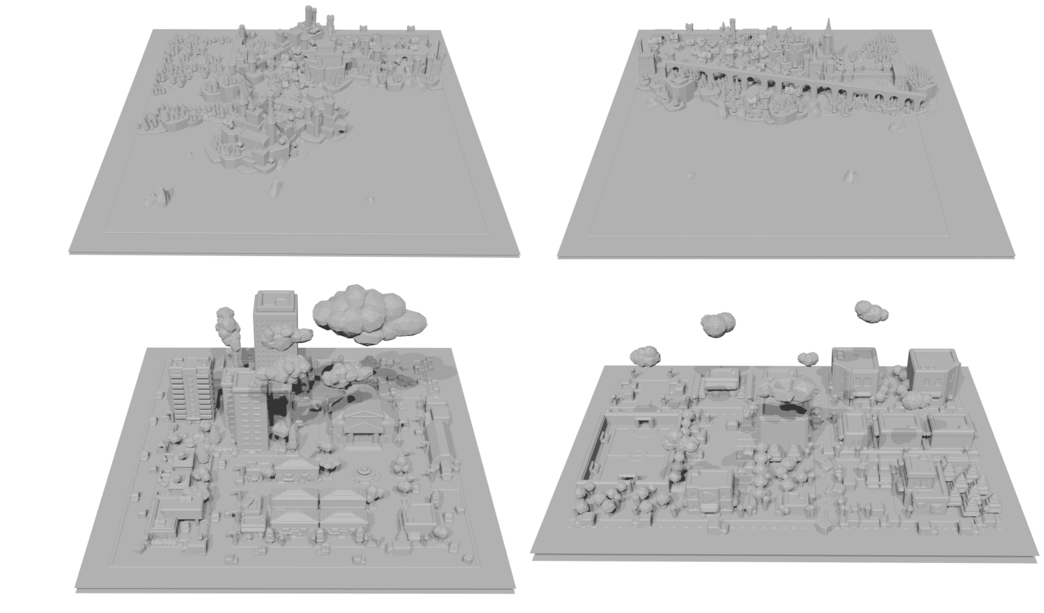
Figure 10: Three additional scenes used to train our multi-scene model. The top two sub-scenes were split from the same scene in Objaverse for occupancy calculation. The shown scenes have been processed with fixed ground geometries, and their meshes were extracted using the marching cubes algorithm on the occupancy grid.

Appendix S1 NuiScene43 Dataset

We obtain training scenes from Objaverse by applying several rounds of filtering, ultimately selecting 43 high quality moderately to large sized scenes (S1.1). To ensure a unified scale between scenes, we annotate scenes with scales relative to each other, aligning them under a uniform scale (S1.2). Finally, we preprocess the raw Objaverse mesh files for training by sampling point clouds, adjusting ground geometry, and converting them to occupancies (S1.3). Furthermore, we describe the sampling maps used to sample quad chunks from scenes (S1.4) as well as some dataset statistics (S1.5).

S1.1 Filtering

We begin by filtering Objaverse [9] using multi-view embeddings from DuoduoCLIP [24]. We use cosine similarity to query embeddings and retrieve objects, then refine selection through manual labeling and neural network filtering trained on DuoduoCLIP embeddings, reducing 37k initial scenes to 2k. Since manually processing all scenes for scale labeling and ground alignment is impractical, we select 43 larger scenes for initial experiments, which we refer to as the NuiScene43 dataset.

S1.2 Scale Labeling

To establish a uniform scale across scenes, we first normalize all scenes to be within the $[-1,1]$ range. We then randomly select one scene as the anchor, assigning it a scale of 1. Each remaining scene is compared side by side with the anchor, and its scale is adjusted visually to align elements such as trees or buildings from multiple angles, to ensure a visually coherent relative size. Since these scenes are artist-created, their proportions may prioritize aesthetic appeal over real-world accuracy. As a result, there is no definitive correct scale. Instead, we approximate a visually consistent scaling and record the assigned scale for each scene, with the anchor scene remaining fixed at scale 1.

S1.3 Geometry Processing

Point Cloud and Occupancy. All scene meshes are first converted into SDFs using the same method as Wang et al. [40], re-implemented in Taichi [16] for faster conversion. The scales obtained in S1.2 are used to adjust the voxel grid resolution for SDF conversion to enforce the unified scale across scenes. We then convert to occupancy by thresholding SDF values at zero. Finally, we apply multiple iterations of flood filling to fill in holes in the scene. Point clouds are sampled from the meshes after applying the Marching Cubes algorithm to the occupancy of each scene.

Ground Fixing. We observed that the filtered scenes had various ground geometry, ranging from flat planes to thick volumes. To deal with this, we identify the lowest ground level in each scene and enforce a uniform ground thickness of 5 voxels below this level in the occupancy grid, ensuring consistency in ground geometry across scenes.

S1.4 Chunk Sampling

To sample training chunks from the scenes, we first compute an alpha map from the top-down view of each scene. Next, we apply a convolution with all one kernel weights over the entire scene using a kernel size of $(100,100)$. The resulting convolution map is then thresholded at a value of $100\times 100$ to determine valid sampling locations. This ensures that all sampled chunks contain occupied regions, avoiding holes or boundary areas in the scenes.

Although we define the chunk size as $(50,50)$ along the x and z axes, we actually sample entire 2x2 chunks from the scene. This approach simplifies processing and better accommodates the diffusion model training. For the VAE model, the $(100,100)$ chunks are further divided into four $(50,50)$ chunks for training. An illustration of the sampling map is provided in Figure˜9.

Additionally, we compute a depth variation map. For each pixel, we calculate the mean depth within the kernel window and subtract the pixel’s depth value, taking the absolute value to obtain depth mean deviations. To avoid sampling overly flat regions, we filter out sample locations where the depth variation is below 2.5.

Finally, we apply farthest point sampling (FPS) to select quad chunks from all valid sampling locations. This helps minimize excessive overlap between chunks while ensuring maximum scene coverage for training.

Table 6: NuiScene43 statistics.

Category	# Scenes	# Sampleable Quad Chunks
Rural/Medieval	16	6.2 M
Low Poly City	19	4.9 M
Japanese Buildings	4	2.9 M
Other	4	1.2 M

S1.5 NuiScene43 Statistics

We present statistics of NuiScene43 in Tab.˜6, including the number of scenes in each category and the total number of quad chunks that can be sampled from each category. The chunk count is derived by summing the sampling map discussed earlier, following depth variation thresholding. Note that these chunks may overlap, as we consider all valid x and z coordinates for sampling.

Algorithm 1 Raster Scan Order Scene Generation

1:Number of rows $I$, number of columns $J$, trained diffusion model $\epsilon_{\theta}$

2:Initialize scene latent grid $\bm{Z}\in\mathbb{R}^{I\times J\times V\times c}$

3:for $i=0$ to $I-2$ do $\triangleright$ Iterate row-wise

4:   for $j=0$ to $J-2$ do $\triangleright$ Iterate column-wise

5:     if $i=0$ and $j=0$ then $\triangleright$ First chunk (Full)

6:        $M\leftarrow\{0,0,0,0\}$

7:        $Z_{\text{cond}}\leftarrow\{\mathbf{0},\mathbf{0},\mathbf{0},\mathbf{0}\}$

8:     else if $i=0$ then $\triangleright$ First row (Left-Right)

9:        $M\leftarrow\{1,0,1,0\}$

10:        $Z_{\text{cond}}\leftarrow\{\bm{Z}_{i,j},\mathbf{0},\bm{Z}_{i+1,j},\mathbf{0}\}$

11:     else if $j=0$ then $\triangleright$ First column (Top-Down)

12:        $M\leftarrow\{1,1,0,0\}$

13:        $Z_{\text{cond}}\leftarrow\{\bm{Z}_{i,j},\bm{Z}_{i,j+1},\mathbf{0},\mathbf{0}\}$

14:     else$\triangleright$ All other cases (Diagonal)

15:        $M\leftarrow\{1,1,1,0\}$

16:        $Z_{\text{cond}}\leftarrow\{\bm{Z}_{i,j},\bm{Z}_{i,j+1},\bm{Z}_{i+1,j},\mathbf{0}\}$

17:     end if

18:     $\bm{X}_{t}\sim\mathcal{N}(0,\mathbf{I})$ $\triangleright$ Sample Gaussian noise

19:     $\bm{C}\leftarrow M\oplus Z_{\text{cond}}\oplus\text{PE}$ $\triangleright$ Conditioning input

20:     $\{\bm{z}_{0},\bm{z}_{1},\bm{z}_{2},\bm{z}_{3}\}\leftarrow\epsilon_{\theta}(\bm{X}_{t}\oplus\bm{C},t)$ $\triangleright$ Diffuse 2×2 quad chunk

21:     $\bm{Z}_{i,j},\bm{Z}_{i,j+1},\bm{Z}_{i+1,j},\bm{Z}_{i+1,j+1}\leftarrow\bm{z}_{0},\bm{z}_{1},\bm{z}_{2},\bm{z}_{3}$ $\triangleright$ Write to scene latent grid

22:   end for

23:end for

24:return $\bm{Z}$

Appendix S2 Implementation Details

S2.1 Raster Scan Order Generation

We show the algorithm of our raster scan order generation during inference utilizing our diffusion model trained with 4 different configurations in Algorithm˜1. The algorithm outlines how the 4 different masking configurations are used based on different positions to condition on existing chunks and enable continuous and unbounded generation. After we obtain a large grid of chunks embeddings with Algorithm˜1, the decoder of the VAE is utilized to decode occupancies for the scene chunks. We then use marching cubes to convert the large scene grid of occupancies into the final mesh.

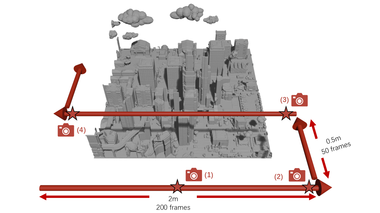
(a) An illustration of our choice for the camera trajectory, indicated by red arrows.

(b) Image rendered at position (1).

(c) Image rendered at position (2).

(d) Image rendered at position (3).

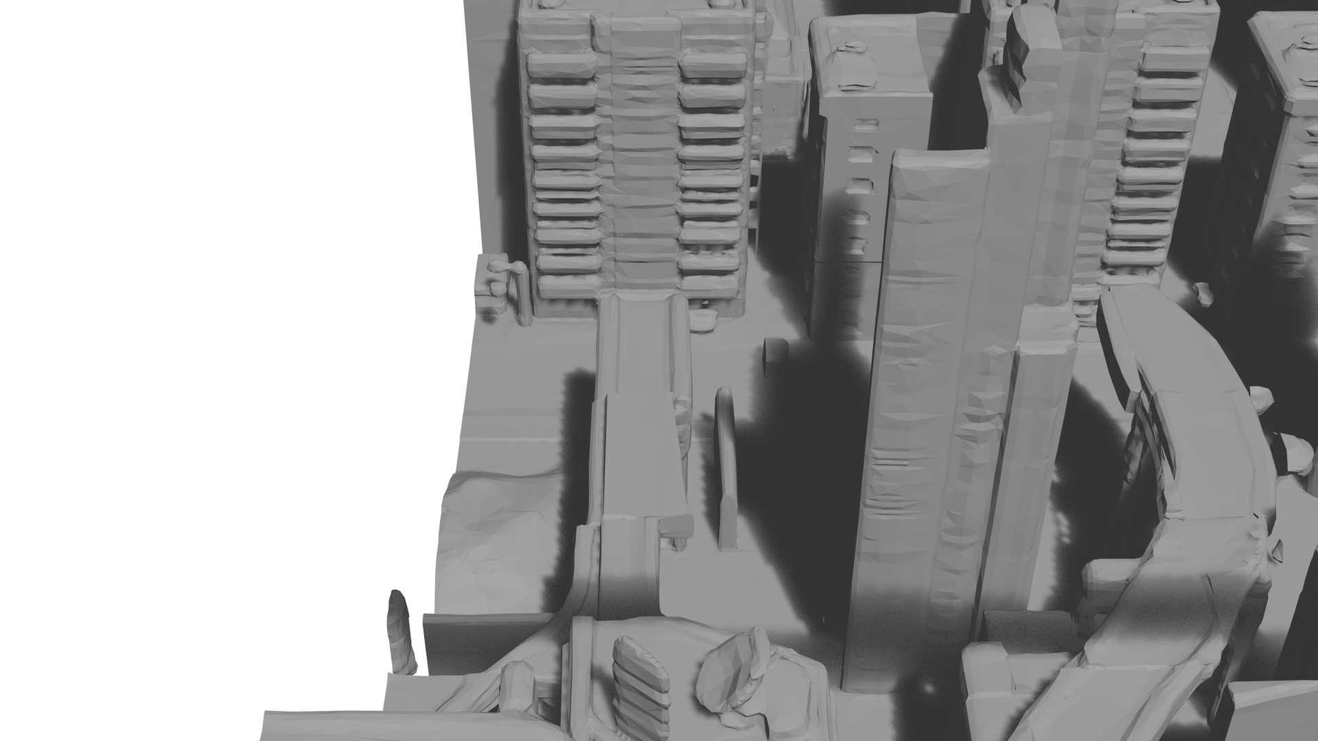
(e) Image rendered at position (4).

Figure 11: An overview of our choice of the camera trajectory in Blender and the four images respectively rendered at position (1), (2), (3) and (4). We adopt a snake-scan trajectory pattern allowing for a more comprehensive coverage of the entire scene. The long side of the trajectory spans 2 meters at a fixed number of 200 frames, and the shorter side spans 0.5 meters for 50 frames. Depending on the shape of the scene, the total number of frames ranges from 1.2k to 1.8k.

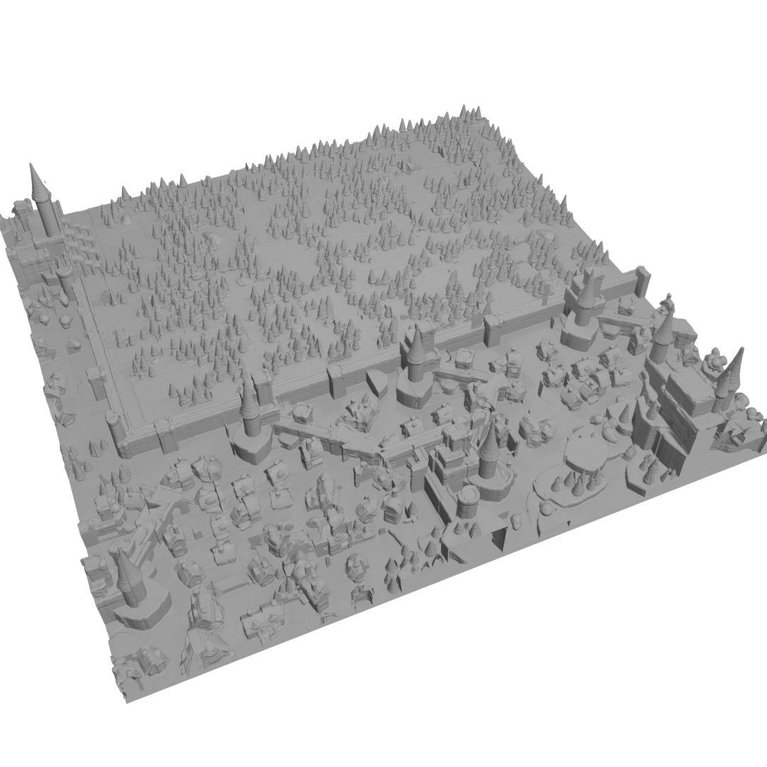
(a) Generated scene (1).

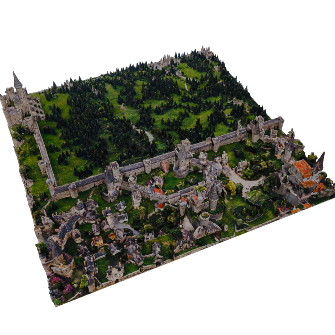
(b) Textured scene (1).

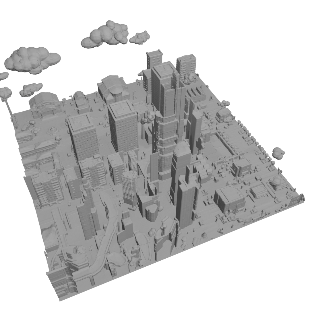
(c) Generated scene (2).

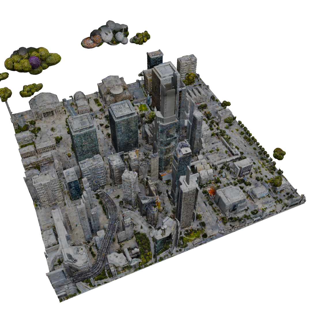
(d) Textured scene (2).

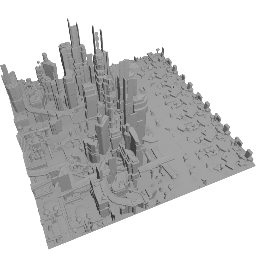
(e) Generated scene (3).

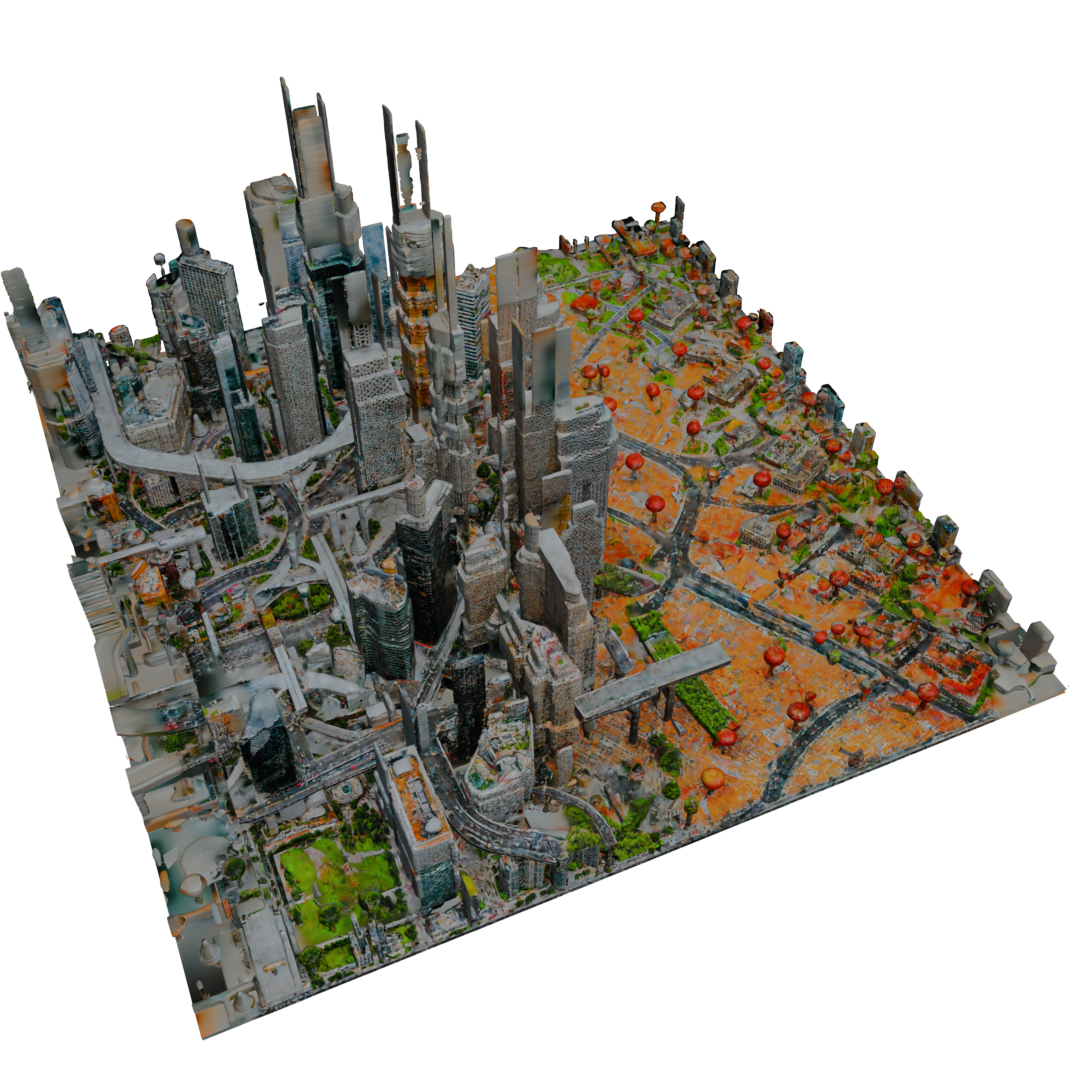
(f) Textured scene (3).

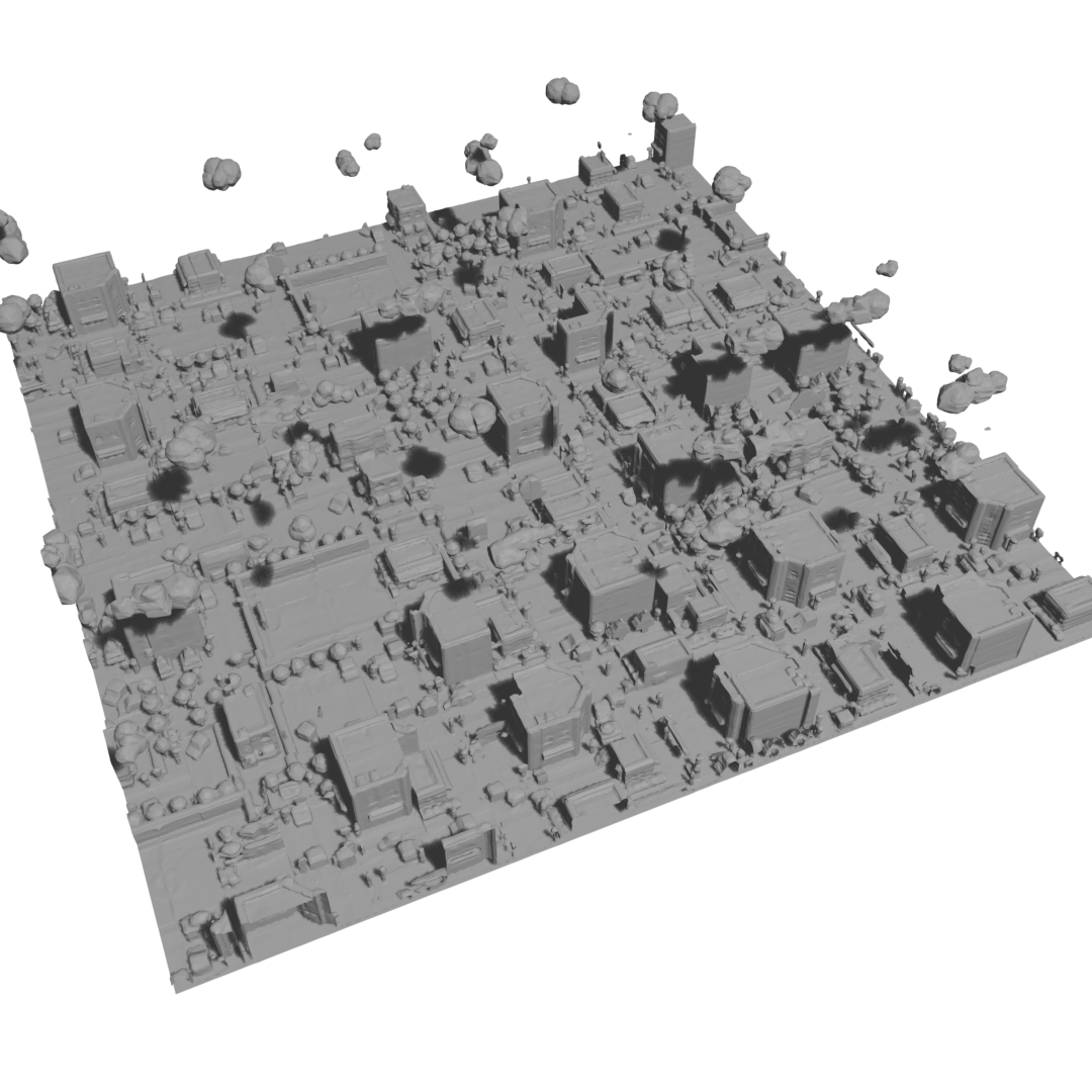
(g) Generated scene (4).

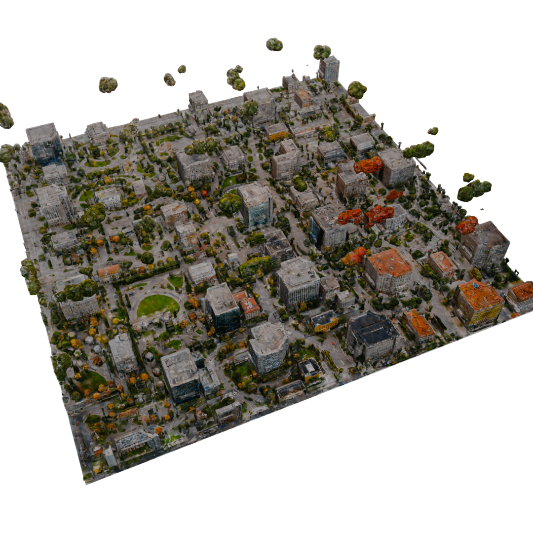
(h) Textured scene (4).

Figure 12: Four examples (1) to (4) of generated scenes and the textured counterparts. (1) is textured using prompt “A beautiful town with buildings, castles and trees”. (2)(3) are textured using prompt “A large city with buildings and surroundings”. (4) is textured using prompt “A modern city with buildings and trees, clouds in the sky”.

S2.2 Multi-scene training

For training the multi-scene model in the paper we add an additional 3 scenes along with the original single scene for training. The additional 3 scenes are shown in Figure˜10.

S2.3 Details on Scene Texturing

SceneTex [6] offers three camera modes for rendering images and texture optimization, i.e., Spherical Cameras, the Blender Cameras and BlenderProc Cameras. For small indoor scenes like those from 3DFront, spherical cameras are sufficient to capture the fine-grained details of the scene and produce high-quality textures. However, for large outdoor scenes, a predefined spherical camera trajectory often fails to cover the entire scene comprehensively and misses important scene details. We therefore choose the Blender Cameras mode to manually keyframe the camera trajectory for each scene. This enables a finer control over capturing the scene details, leading to an improved texture.

More specifically, we first normalize each scene into a spatial range of $[-1,1]^{3}$ centered at the world origin. Then, we define a snake-scan-like camera trajectory to capture the entire scene at a specified frame rate, as shown in Figure˜11. Each frame will be rendered by SceneTex and all rendered images are sampled during training to optimize the scene-level texture. Note that to enable faster optimization, we use Blender’s Decimate Geometry and Merge By Distance with a distance of 0.001m to compress the scene until its size is smaller than 20MB. This might degrade the geometry for large scenes, but it’s only for the texturing purpose. We encourage readers to focus on the untextured geometry details of the generated scenes.

Figure˜12 shows more examples on raw geometries and the textured counterparts.

Appendix S3 Additional Results

S3.1 Single Scene Results

We show additional results from our diffusion model trained on a single scene with vector set backbone in Figure˜13. And additional results for the RePaint baseline in Figure˜14.

S3.1.1 Multi Scene Results

We show additional results from our diffusion model trained on 4 scenes with vector set backbone in Figure˜15 and Figure˜16.

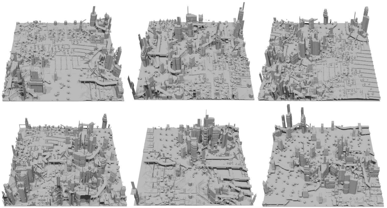
Figure 13: Additional results for our vector set diffusion model trained on a single scene. The scenes shown here are of size $21\times 21$.

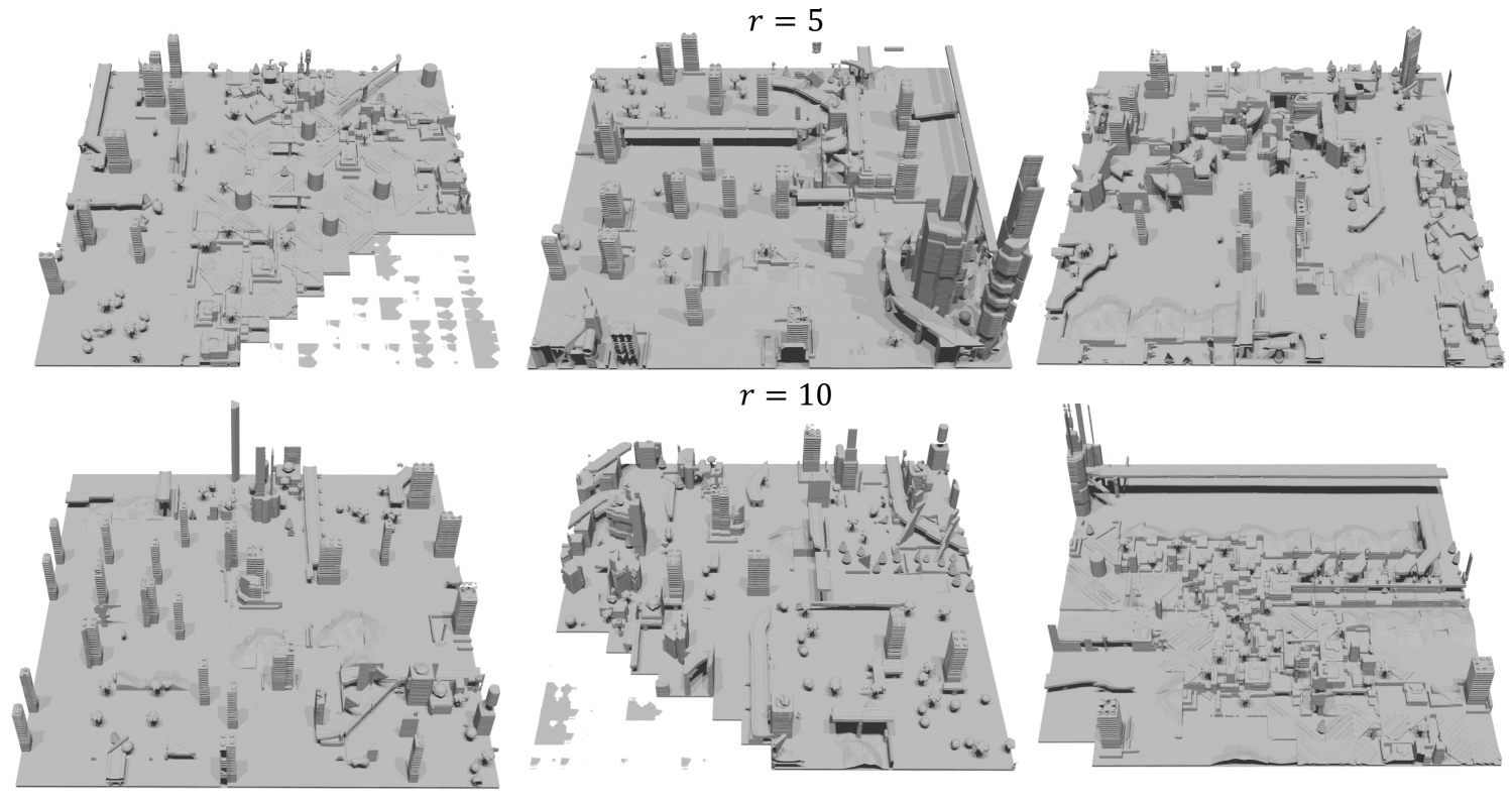
Figure 14: Additional RePaint results using our vector set diffusion model trained on a single scene. The scenes shown here are of size $16\times 16$. We show results for resampling steps $r=5$ and $r=10$. Compared to our outpainting model, RePaint struggles with inter-chunk coherence and sometimes collapses, producing broken chunks in larger scenes.

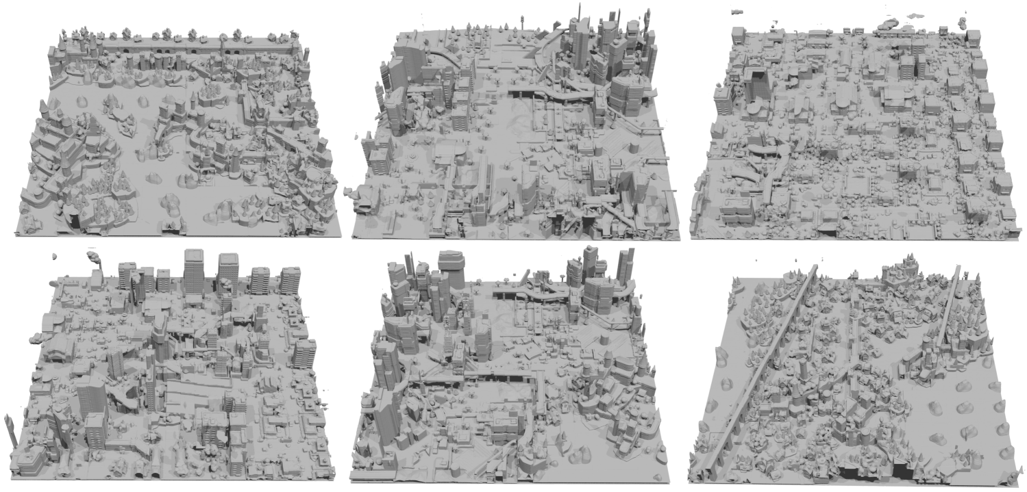
Figure 15: Additional results for our vector set diffusion model trained on multiple scenes. The scenes shown here are of size $21\times 21$.

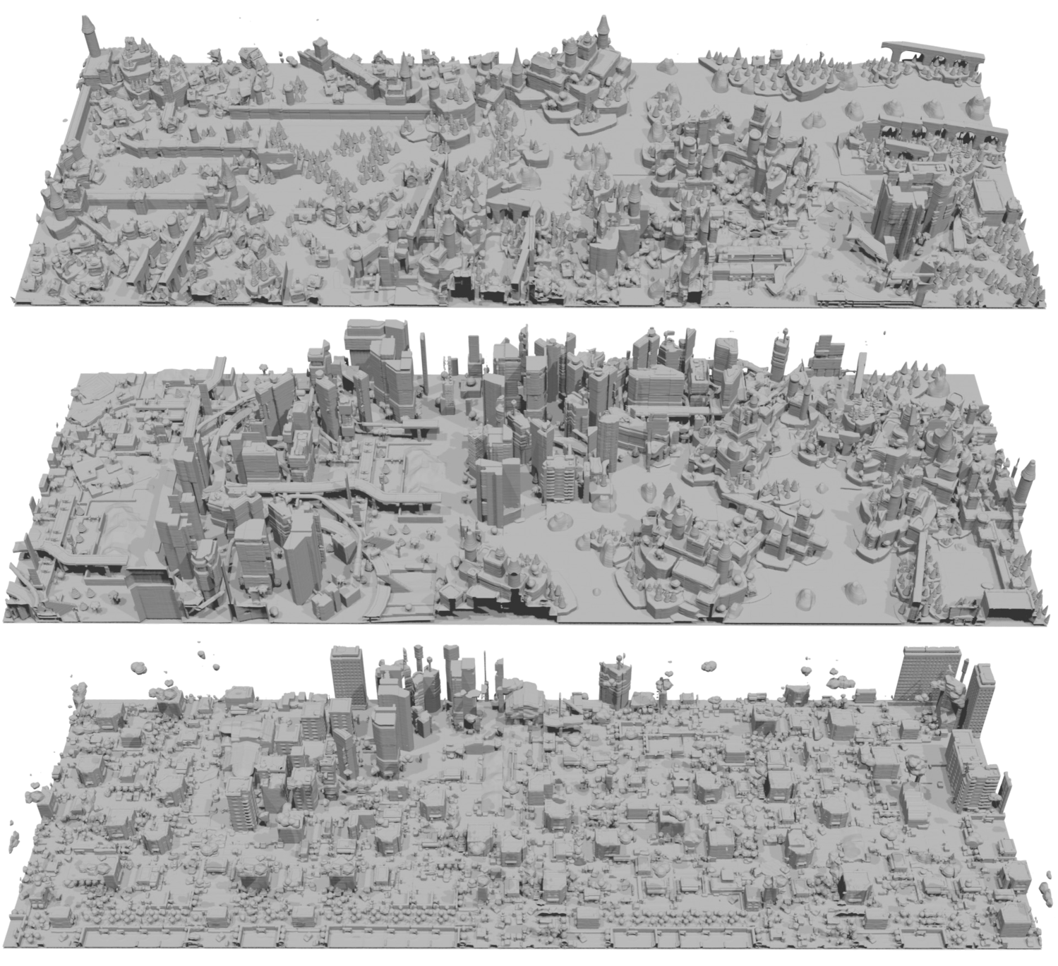
Figure 16: Additional results for our vector set diffusion model trained on a 4 scenes. The scenes shown here are of size $16\times 46$. The scene in the middle is the untextured mesh of Figure˜2.

References

- Achiam et al. [2023] Josh Achiam, Steven Adler, Sandhini Agarwal, Lama Ahmad, Ilge Akkaya, Florencia Leoni Aleman, Diogo Almeida, Janko Altenschmidt, Sam Altman, Shyamal Anadkat, et al. GPT-4 technical report. arXiv preprint arXiv:2303.08774, 2023.
- Behley et al. [2019] Jens Behley, Martin Garbade, Andres Milioto, Jan Quenzel, Sven Behnke, Cyrill Stachniss, and Jurgen Gall. SemanticKITTI: A dataset for semantic scene understanding of lidar sequences. In Proceedings of the IEEE/CVF international conference on computer vision, pages 9297–9307, 2019.
- Bhat et al. [2023] Shariq Farooq Bhat, Reiner Birkl, Diana Wofk, Peter Wonka, and Matthias Müller. ZoeDepth: Zero-shot transfer by combining relative and metric depth. arXiv preprint arXiv:2302.12288, 2023.
- Bokhovkin et al. [2024] Alexey Bokhovkin, Quan Meng, Shubham Tulsiani, and Angela Dai. SceneFactor: Factored latent 3D diffusion for controllable 3D scene generation. arXiv preprint arXiv:2412.01801, 2024.
- Chai et al. [2023] Lucy Chai, Richard Tucker, Zhengqi Li, Phillip Isola, and Noah Snavely. Persistent nature: A generative model of unbounded 3D worlds. In Proceedings of the IEEE/CVF conference on computer vision and pattern recognition, pages 20863–20874, 2023.
- Chen et al. [2024] Dave Zhenyu Chen, Haoxuan Li, Hsin-Ying Lee, Sergey Tulyakov, and Matthias Nießner. SceneTex: High-quality texture synthesis for indoor scenes via diffusion priors. In Proceedings of the IEEE/CVF Conference on Computer Vision and Pattern Recognition, pages 21081–21091, 2024.
- Chen et al. [2023] Zhaoxi Chen, Guangcong Wang, and Ziwei Liu. SceneDreamer: Unbounded 3D scene generation from 2D image collections. IEEE transactions on pattern analysis and machine intelligence, 45(12):15562–15576, 2023.
- Chung et al. [2023] Jaeyoung Chung, Suyoung Lee, Hyeongjin Nam, Jaerin Lee, and Kyoung Mu Lee. LucidDreamer: Domain-free generation of 3D Gaussian splatting scenes. arXiv preprint arXiv:2311.13384, 2023.
- Deitke et al. [2023] Matt Deitke, Dustin Schwenk, Jordi Salvador, Luca Weihs, Oscar Michel, Eli VanderBilt, Ludwig Schmidt, Kiana Ehsani, Aniruddha Kembhavi, and Ali Farhadi. Objaverse: A universe of annotated 3D objects. In Proceedings of the IEEE/CVF Conference on Computer Vision and Pattern Recognition, pages 13142–13153, 2023.
- Fridman et al. [2023] Rafail Fridman, Amit Abecasis, Yoni Kasten, and Tali Dekel. SceneScape: Text-driven consistent scene generation. Advances in Neural Information Processing Systems, 36:39897–39914, 2023.
- Fu et al. [2021] Huan Fu, Bowen Cai, Lin Gao, Ling-Xiao Zhang, Jiaming Wang, Cao Li, Qixun Zeng, Chengyue Sun, Rongfei Jia, Binqiang Zhao, et al. 3D-front: 3D furnished rooms with layouts and semantics. In Proceedings of the IEEE/CVF International Conference on Computer Vision, pages 10933–10942, 2021.
- Gao et al. [2024] Lin Gao, Yu Liu, Xi Chen, Yuxiang Liu, Shen Yan, and Maojun Zhang. CUS3D: A new comprehensive urban-scale semantic-segmentation 3D benchmark dataset. Remote Sensing, 16(6):1079, 2024.
- Gao et al. [2021] Weixiao Gao, Liangliang Nan, Bas Boom, and Hugo Ledoux. SUM: A benchmark dataset of semantic urban meshes. ISPRS Journal of Photogrammetry and Remote Sensing, 179:108–120, 2021.
- Ho et al. [2020] Jonathan Ho, Ajay Jain, and Pieter Abbeel. Denoising diffusion probabilistic models. Advances in neural information processing systems, 33:6840–6851, 2020.
- Hong et al. [2023] Yicong Hong, Kai Zhang, Jiuxiang Gu, Sai Bi, Yang Zhou, Difan Liu, Feng Liu, Kalyan Sunkavalli, Trung Bui, and Hao Tan. LRM: Large reconstruction model for single image to 3D. arXiv preprint arXiv:2311.04400, 2023.
- Hu et al. [2019] Yuanming Hu, Tzu-Mao Li, Luke Anderson, Jonathan Ragan-Kelley, and Frédo Durand. Taichi: a language for high-performance computation on spatially sparse data structures. ACM Transactions on Graphics (TOG), 38(6):201, 2019.
- Ju et al. [2024] Xiaoliang Ju, Zhaoyang Huang, Yijin Li, Guofeng Zhang, Yu Qiao, and Hongsheng Li. DiffInDScene: Diffusion-based high-quality 3D indoor scene generation. In Proceedings of the IEEE/CVF Conference on Computer Vision and Pattern Recognition, pages 4526–4535, 2024.
- Karnewar et al. [2022] Animesh Karnewar, Oliver Wang, Tobias Ritschel, and Niloy J Mitra. 3inGAN: Learning a 3D generative model from images of a self-similar scene. In 2022 International Conference on 3D Vision (3DV), pages 342–352. IEEE, 2022.
- Ke et al. [2024] Bingxin Ke, Anton Obukhov, Shengyu Huang, Nando Metzger, Rodrigo Caye Daudt, and Konrad Schindler. Repurposing diffusion-based image generators for monocular depth estimation. In Proceedings of the IEEE/CVF Conference on Computer Vision and Pattern Recognition, pages 9492–9502, 2024.
- Kingma et al. [2013] Diederik P Kingma, Max Welling, et al. Auto-encoding variational bayes, 2013.
- Kirillov et al. [2023] Alexander Kirillov, Eric Mintun, Nikhila Ravi, Hanzi Mao, Chloe Rolland, Laura Gustafson, Tete Xiao, Spencer Whitehead, Alexander C Berg, Wan-Yen Lo, et al. Segment anything. In Proceedings of the IEEE/CVF international conference on computer vision, pages 4015–4026, 2023.
- Lasinger et al. [2019] Katrin Lasinger, René Ranftl, Konrad Schindler, and Vladlen Koltun. Towards robust monocular depth estimation: Mixing datasets for zero-shot cross-dataset transfer. arXiv preprint arXiv:1907.01341, 2019.
- Lee et al. [2024a] Hanhung Lee, Manolis Savva, and Angel X Chang. Text-to-3d shape generation. In Computer Graphics Forum, page e15061. Wiley Online Library, 2024a.
- Lee et al. [2024b] Han-Hung Lee, Yiming Zhang, and Angel X Chang. Duoduo CLIP: Efficient 3D understanding with multi-view images. arXiv preprint arXiv:2406.11579, 2024b.
- Lee et al. [2023] Jumin Lee, Woobin Im, Sebin Lee, and Sung-Eui Yoon. Diffusion probabilistic models for scene-scale 3D categorical data. arXiv preprint arXiv:2301.00527, 2023.
- Lee et al. [2024c] Jumin Lee, Sebin Lee, Changho Jo, Woobin Im, Juhyeong Seon, and Sung-Eui Yoon. SemCity: Semantic scene generation with triplane diffusion. In Proceedings of the IEEE/CVF conference on computer vision and pattern recognition, pages 28337–28347, 2024c.
- Li et al. [2023] Weiyu Li, Xuelin Chen, Jue Wang, and Baoquan Chen. Patch-based 3D natural scene generation from a single example. In Proceedings of the IEEE/CVF Conference on Computer Vision and Pattern Recognition, pages 16762–16772, 2023.
- Li et al. [2024] Weiyu Li, Jiarui Liu, Rui Chen, Yixun Liang, Xuelin Chen, Ping Tan, and Xiaoxiao Long. Craftsman: High-fidelity mesh generation with 3d native generation and interactive geometry refiner. arXiv preprint arXiv:2405.14979, 2024.
- Lin et al. [2023] Chieh Hubert Lin, Hsin-Ying Lee, Willi Menapace, Menglei Chai, Aliaksandr Siarohin, Ming-Hsuan Yang, and Sergey Tulyakov. InfiniCity: Infinite-scale city synthesis. In Proceedings of the IEEE/CVF international conference on computer vision, pages 22808–22818, 2023.
- Liu et al. [2024] Yuheng Liu, Xinke Li, Xueting Li, Lu Qi, Chongshou Li, and Ming-Hsuan Yang. Pyramid diffusion for fine 3D large scene generation. In European Conference on Computer Vision, pages 71–87. Springer, 2024.
- Lugmayr et al. [2022] Andreas Lugmayr, Martin Danelljan, Andres Romero, Fisher Yu, Radu Timofte, and Luc Van Gool. Repaint: Inpainting using denoising diffusion probabilistic models. In Proceedings of the IEEE/CVF conference on computer vision and pattern recognition, pages 11461–11471, 2022.
- Meng et al. [2024] Quan Meng, Lei Li, Matthias Nießner, and Angela Dai. LT3SD: Latent trees for 3D scene diffusion. arXiv preprint arXiv:2409.08215, 2024.
- Nichol et al. [2022] Alex Nichol, Heewoo Jun, Prafulla Dhariwal, Pamela Mishkin, and Mark Chen. Point-e: A system for generating 3d point clouds from complex prompts. arXiv preprint arXiv:2212.08751, 2022.
- Qi et al. [2017] Charles Ruizhongtai Qi, Li Yi, Hao Su, and Leonidas J Guibas. Pointnet++: Deep hierarchical feature learning on point sets in a metric space. Advances in neural information processing systems, 30, 2017.
- Riemenschneider et al. [2014] Hayko Riemenschneider, András Bódis-Szomorú, Julien Weissenberg, and Luc Van Gool. Learning where to classify in multi-view semantic segmentation. In Computer Vision–ECCV 2014: 13th European Conference, Zurich, Switzerland, September 6-12, 2014, Proceedings, Part V 13, pages 516–532. Springer, 2014.
- Rombach et al. [2022] Robin Rombach, Andreas Blattmann, Dominik Lorenz, Patrick Esser, and Björn Ommer. High-resolution image synthesis with latent diffusion models. In Proceedings of the IEEE/CVF conference on computer vision and pattern recognition, pages 10684–10695, 2022.
- Shaham et al. [2019] Tamar Rott Shaham, Tali Dekel, and Tomer Michaeli. SinGAN: Learning a generative model from a single natural image. In Proceedings of the IEEE/CVF international conference on computer vision, pages 4570–4580, 2019.
- Shriram et al. [2024] Jaidev Shriram, Alex Trevithick, Lingjie Liu, and Ravi Ramamoorthi. RealmDreamer: Text-driven 3D scene generation with inpainting and depth diffusion. arXiv preprint arXiv:2404.07199, 2024.
- Van Den Oord et al. [2017] Aaron Van Den Oord, Oriol Vinyals, et al. Neural discrete representation learning. Advances in neural information processing systems, 30, 2017.
- Wang et al. [2022] Peng-Shuai Wang, Yang Liu, and Xin Tong. Dual octree graph networks for learning adaptive volumetric shape representations. ACM Transactions on Graphics (TOG), 41(4):1–15, 2022.
- Wang et al. [2024] Yu-Jie Wang, Xue-Lin Chen, and Bao-Quan Chen. SinGRAV: Learning a generative radiance volume from a single natural scene. Journal of Computer Science and Technology, 39(2):305–319, 2024.
- Wilson et al. [2022] Joey Wilson, Jingyu Song, Yuewei Fu, Arthur Zhang, Andrew Capodieci, Paramsothy Jayakumar, Kira Barton, and Maani Ghaffari. MotionSC: Data set and network for real-time semantic mapping in dynamic environments. IEEE Robotics and Automation Letters, 7(3):8439–8446, 2022.
- Wu and Zheng [2022] Rundi Wu and Changxi Zheng. Learning to generate 3D shapes from a single example. arXiv preprint arXiv:2208.02946, 2022.
- Wu et al. [2024] Zhennan Wu, Yang Li, Han Yan, Taizhang Shang, Weixuan Sun, Senbo Wang, Ruikai Cui, Weizhe Liu, Hiroyuki Sato, Hongdong Li, et al. BlockFusion: Expandable 3D scene generation using latent tri-plane extrapolation. ACM Transactions on Graphics (TOG), 43(4):1–17, 2024.
- Xiang et al. [2024] Jianfeng Xiang, Zelong Lv, Sicheng Xu, Yu Deng, Ruicheng Wang, Bowen Zhang, Dong Chen, Xin Tong, and Jiaolong Yang. Structured 3d latents for scalable and versatile 3d generation. arXiv preprint arXiv:2412.01506, 2024.
- Xie et al. [2024] Haozhe Xie, Zhaoxi Chen, Fangzhou Hong, and Ziwei Liu. CityDreamer: Compositional generative model of unbounded 3D cities. In CVPR, 2024.
- Yan et al. [2024] Xingguang Yan, Han-Hung Lee, Ziyu Wan, and Angel X Chang. An object is worth 64x64 pixels: Generating 3d object via image diffusion. arXiv preprint arXiv:2408.03178, 2024.
- Yu et al. [2024] Hong-Xing Yu, Haoyi Duan, Charles Herrmann, William T Freeman, and Jiajun Wu. WonderWorld: Interactive 3D scene generation from a single image. arXiv preprint arXiv:2406.09394, 2024.
- Zhang et al. [2023] Biao Zhang, Jiapeng Tang, Matthias Niessner, and Peter Wonka. 3DShape2VecSet: A 3D shape representation for neural fields and generative diffusion models. ACM Transactions on Graphics (TOG), 42(4):1–16, 2023.