Impact of the Intraspecies Scattering Length on the
Observability of Resonances in Efimov-Unfavored Systems

Abstract

Efimov resonances in the three-body loss rate have been observed in ultracold heteronuclear gases near interspecies Feshbach resonances. However, the intraspecies scattering length $a_{\text{BB}}$ has been assumed to have a negligible effect on the overall Efimov scenario, namely, on the locations of the Efimov resonances $a_{-}^{(n)}$ and, consequently, on the three-body parameter (3BP). The present Letter analyzes the influence of $a_{\text{BB}}$ on the Efimov resonance positions $a_{-}^{(n)}$, particularly the 3BP, in Efimov-unfavored systems. Using van der Waals interactions described by separable $s$-wave potentials, the unitarity energy spectrum ($\absolutevalue{a_{\text{BX}}}\rightarrow\infty$) and the Efimov resonance positions $a_{-}^{(n)}$ for $\ch{{}^{23}Na2^{40}K}$ are mapped out in $a_{\text{BB}}$. It is found that both the magnitude and sign of $a_{\text{BB}}$ can significantly impact the resonances $a_{-}^{(n)}$ in Efimov-unfavored systems, with the 3BP taking an observable value when $a_{\text{BB}}<0$.

The ability to fully tune the interactions strength—i.e., vary the scattering length $a$—using an external magnetic field [1, 2] in systems supporting Feshbach resonances has enabled ultracold experiments to access the regime of the Efimov effect [3]. Subsequently, theoretical interest in Efimov physics has grown substantially [4, 5, 6, 7, 8, 9, 10, 11], owing to its crucial role in understanding and controlling atomic losses in ultracold experiments. Efimov states have been extensively observed in homonuclear systems [12, 13, 14, 15, 16, 17, 18, 19, 20, 21, 22, 23, 24, 25, 26], as $a$ is varied across a Feshbach resonance, through their signatures in the three-body loss rate $K_{3}$, appearing as resonances for $a<0$ and minima for $a>0$. Efimov resonances occur in $K_{3}$ at negative scattering lengths, denoted $a_{-}^{(n)}$, when distinct Efimov trimers reach the three-body threshold, forming a shape resonance that serves as an enhancing intermediate state for ultracold three-body recombination (3BR) [27]. Although the Efimov series extends infinitely toward the three-body threshold, it is bounded from below by the physics at short interparticle distances through a three-body parameter (3BP) [5]. Standard choices for the 3BP include the ground state energy $E_{0}$ at unitarity and the scattering length $a_{-}^{(0)}$ of the first Efimov resonance.

While the Efimov effect is primarily known for three identical atoms, it also occurs in heteronuclear systems (BBX) composed of two identical bosons and a distinguishable atom, provided that at least two pairs are resonant (i.e., the interspecies scattering length $\absolutevalue{a_{\text{BX}}}\rightarrow\infty$) [28, 29, 30, 31, 32, 33]. In these systems, two Efimov scaling parameters arise depending on whether only two ($s_{0}$) or all three ($s_{0}^{*}$) pairs are resonant, both determined by the system mass imbalance [10]. Efimov resonances $a_{-}^{(n)}$ have been reported in ultracold two-species gases [34, 35, 36, 37, 38] as $a_{\text{BX}}$ is varied near an interspecies Feshbach resonance, thereby measuring the 3BP $a_{-}^{(0)}$. “Efimov-favored” systems, involving two extremely heavy and one light atom, feature a small Efimov spacing ($s_{0}>1$), enabling the detection of multiple states in the geometric series [37, 38], in contrast to “Efimov-unfavored” systems ($s_{0}<1$).

Nonetheless, in most studies, the intraspecies scattering length $a_{\text{BB}}$ has been treated as a background parameter with no significant influence on the locations of the Efimov resonances $a_{-}^{(n)}$ or, in particular, on the 3BP. For instance, Wang et al. [31, 32] reported the 3BP for multiple mass ratios, each at a single positive $a_{\text{BB}}$, with an excessively large $|a_{-}^{(0)}|$ in the Efimov-unfavored cases. A glimpse of this influence was revealed in the $\ch{Cs2Li}$ system, where the ground-state Efimov resonance was found to be absent for $a_{\text{BB}}>0$ due to the $\ch{Cs2}\,+\,\ch{Li}$ threshold, resulting in different 3BPs for opposite signs of $a_{\text{BB}}$ [39, 40]. In Efimov-unfavored systems, however, $a_{\text{BB}}$ is expected to have a more prominent effect, as suggested by the large discrepancy between $s_{0}$ and $s_{0}^{*}$ [10], highlighting the significance of the intraspecies interaction. In particular, we show that an observable value of the 3BP can occur even in an Efimov-unfavored system, provided the value of $a_{\text{BB}}$ is negative.

This Letter investigates the dependence of the 3BP as well as the Efimov resonances $a_{-}^{(n)}$ on $a_{\text{BB}}$ in Efimov-unfavored systems. Using a finite-range model for $\ch{{}^{23}Na2^{40}K}$, a recently observed example [41], it is found that $a_{\text{BB}}$ can drastically affect both the unitarity energy spectrum ($\absolutevalue{a_{\text{BX}}}\rightarrow\infty$) and the Efimov resonance positions $a_{-}^{(n)}$. Specifically, we identify distinct mechanisms through which the Efimov spectrum (and the associated $a_{-}^{(n)}$) is controlled by $a_{\text{BB}}$, depending on its sign. For $a_{\text{BB}}<0$, a strong variation of the unitarity spectrum manifests in the intermediate regime, where the homonuclear pair becomes “partially” resonant as the system transitions from three to two resonant pairs. Conversely, for $a_{\text{BB}}>0$, a similar yet dramatically more pronounced effect than in the Cs-Cs-Li Refs. [39, 40] leads to the absence of an entire series of Efimov resonances, rather than just one, yielding a notably different 3BP compared to the case of $a_{\text{BB}}<0$. These mechanisms, revealed by the finite-range model, are interpreted and supported by zero-range hyperspherical potential curves.

The Schrödinger equation in momentum space for three distinguishable particles reads

$$\left(\frac{\hbar^{2}p_{i}^{2}}{2\mu^{i}}+\frac{\hbar^{2}q_{i}^{2}}{2\mu_{i}}\right)\Psi(\vec{p}_{i},\vec{q}_{i})\;+\\ \sum_{j=1}^{3}\int\frac{d^{3}\vec{q}_{j}\!^{\prime}}{(2\pi)^{3}}V_{j}(\vec{q}_{j},\vec{q}_{j}\!^{\prime})\Psi(\vec{p}_{j},\vec{q}_{j}\!^{\prime})=E\,\Psi(\vec{p}_{i},\vec{q}_{i}),$$ (1)

where $(\vec{p}_{i},\vec{q}_{i})$ are the usual Jacobi momenta. The two-body interactions are assumed to be described by separable $s$-wave potentials [42]:

$$V_{i}(\vec{q},\vec{q}\,^{\prime})=\frac{\hbar^{2}}{2\mu_{i}}\alpha_{i}\ \chi_{i}(q)\chi^{*}_{i}(q^{\prime}).$$ (2)

Following Naidon et al. [43], our treatment adopts the following form factors modeling van der Waals interactions

$$\chi_{i}(q)=1-q\int_{0}^{\infty}\left(1-\frac{r}{a_{i}}-\varphi_{i}(r)\right)\sin(qr)\,dr,$$ (3)

and the prefactors $\alpha_{i}$ are selected as

$$\frac{1}{\alpha_{i}}=\frac{1}{4\pi a_{i}}-\frac{1}{2\pi^{2}}\int_{0}^{\infty}dq\absolutevalue{\chi_{i}(q)}^{2},$$ (4)

where $a_{i}$ are the $s$-wave scattering lengths and $\varphi(r)$ is the zero-energy $s$-wave radial solution of the van der Waals potential. Inserting the separable potentials (Eq. (2)) in Eq. (1) leads to a system of coupled integral equations in the unknowns $F_{i}$

$$D_{i}(p)F_{i}(p)+\sum_{j\neq i}\int_{0}^{\infty}H_{ij}(p,q)F_{j}(q)\,dq=0.$$ (5)

The functions $D_{i}$ and $H_{ij}$ are given by

$$D_{i}(p)=\mu_{i}\left(\frac{\pi}{a_{i}}-2\left(\frac{p^{2}}{\mu^{i}}-\frac{2E}{\hbar^{2}}\right)\int_{0}^{\infty}\frac{\absolutevalue{\chi_{i}(q)}^{2}dq}{\frac{q^{2}}{\mu_{i}}+\frac{p^{2}}{\mu^{i}}-\frac{2E}{\hbar^{2}}}\right),$$ (6)

$$H_{ij}(p,q)=\int_{-1}^{1}du\,P_{L}(u)\,q^{2}\\ \times\frac{\chi^{*}_{i}\!\left(\absolutevalue{\vec{q}+\frac{m_{j}}{m_{j}+m_{k}}\vec{p}\,}\right)\chi_{j}\!\left(\absolutevalue{\vec{p}+\frac{m_{i}}{m_{i}+m_{k}}\vec{q}\,}\right)}{\frac{p^{2}}{\mu_{j}}+\frac{q^{2}}{\mu_{i}}+\frac{2}{m_{k}}pqu-\frac{2E}{\hbar^{2}}},$$ (7)

where $P_{L}(u)$ is a Legendre polynomial. The allowed trimer energies $E$ are found by solving the determinantal equation, obtained from discretizing the system, for any scattering lengths $a_{i}$, masses $m_{i}$, and a total angular momentum $L$ [44]. For a BBX system (our case of interest) the required symmetry constraint is $F_{2}=F_{1}$, simplifying the original $3\times 3$ system in Eqs. (5) to a $2\times 2$ system. Note that instead of searching for roots in energy $E$ at a fixed set of scattering lengths $a_{i}$, one can search for roots in scattering lengths at a given energy. This approach proves useful in determining the values $a_{-}^{(n)}$ by solving the determinantal equation for $a_{\text{BX}}$ at the three-body threshold ($E=0$) while fixing $a_{\text{BB}}$.

The two van der Waals lengths used for ^23Na2^40K are $\ell_{\text{BB}}=45$ a.u. and $\ell_{\text{BX}}=53.6$ a.u. [45, 46]. Eqs. (5) are solved for the energies of spherically symmetric trimer states ($L=0$) over a range of values for one scattering length ($a_{\text{BB}}$ or $a_{\text{BX}}$) with the other held fixed. Results associated with Eqs. (5) are henceforth referred to as finite-range (FR) calculations. The results of FR calculations in momentum space are compared with those from real-space calculations based on adiabatic potential curves with contact $s$-wave interactions. The zero-range hyperspherical potential curves are given by

$$U_{n}(R)=\frac{\hbar^{2}}{2\mu}\left[\frac{\lambda_{n}(R)-1/4}{R^{2}}-Q_{nn}(R)\right],$$ (8)

where $Q_{nn}$ represents the nonadiabatic diagonal corrections. The hyperangular eigenvalues $\lambda_{n}$ are computed as the determinantal roots (at each $R$) of a $3\times 3$ ($2\times 2$ for BBX) matrix $\text{Z}_{a_{i},m_{i}}^{R,L}(\lambda)$, whose elements are analytically known for any scattering lengths $a_{i}$, masses $m_{i}$, and a total angular momentum $L$ [47]. Upon generating the pertinent three-body potential curves, one can look for three-body bound states associated with each adiabatic potential. Results derived from this model are subsequently referred to as zero-range (ZR) calculations.

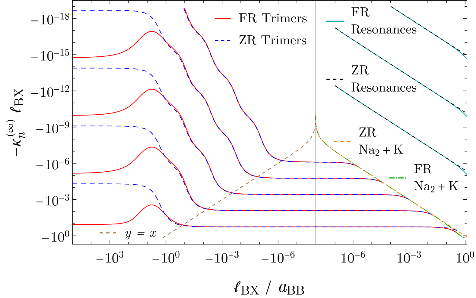
Figure 1: The Efimov spectrum for ^23Na2^40K at heteronuclear unitarity ($\absolutevalue{a_{\text{BX}}}\rightarrow\infty$) with $\kappa_{n}=\sqrt{-m_{\text{B}}E_{n}}/\hbar$. Each plotted quantity is computed from both a finite-range and a zero-range calculation. The dimer threshold (green and orange) divides the spectrum into lower trimers (red and blue) and upper resonances (cyan and black).

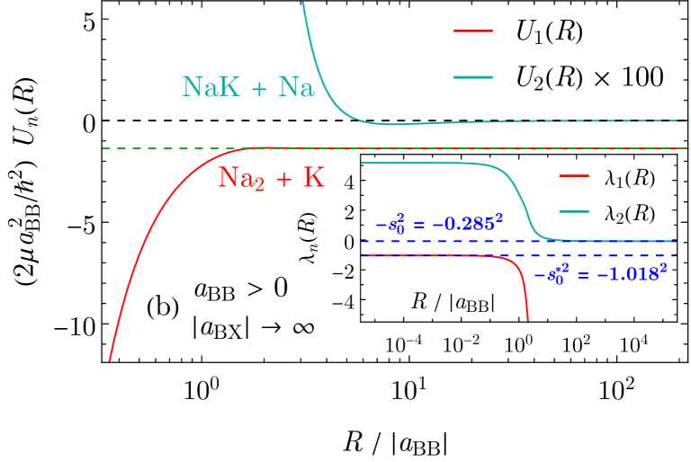
Figure 2: The zero-range hyperspherical potentials $U_{n}(R)$ at heteronuclear unitarity ($\absolutevalue{a_{\text{BX}}}\rightarrow\infty$), shown for $a_{\text{BB}}<0$ (a) and $a_{\text{BB}}>0$ (b). The insets display the corresponding hyperangular eigenvalues $\lambda_{n}(R)$ defined in Eq. 8. In the right panel, the upper potential $U_{2}(R)$ (cyan) is magnified by a factor of 100 for better visibility.

The (rescaled) energies of the lowest several Efimov states at $\absolutevalue{a_{\text{BX}}}\rightarrow\infty$, as well as the Na2 dimer threshold, are displayed in Fig. 1 as functions of $1/a_{\text{BB}}$. While solving the hyperradial Schrödinger equation with the ZR potential (Eq. (8)) at $\absolutevalue{a_{\text{BB}}}\rightarrow\infty$, a short-range log-derivative was chosen to match an eigenvalue to the FR model’s ground state energy. This log-derivative was then fixed for the ZR calculations at other $a_{\text{BB}}$ values. For $a_{\text{BB}}<0$, the spectrum follows an Efimov geometric scaling in two main regions, with the ratios of successive energies being relatively small around $a_{\text{BB}}\rightarrow-\infty$ and gradually increasing to a much larger value as $a_{\text{BB}}\rightarrow 0^{-}$. Moving leftward from $1/a_{\text{BB}}=0$, Efimov states enter an “intermediate region” where they oscillate while progressively rising until the new scaling is achieved. The boundaries of this intermediate region differ for each state, as more excited states rise earlier than deeper ones.

The rationale behind that behavior can be understood by examining the relevant ZR potential curves and their dependence on $a_{\text{BB}}$. As evident in the inset of Fig. 2(a), for $a_{\text{BB}}<0$, the hyperangular eigenvalue $\lambda_{1}(R)$, which controls the Efimov scaling (see Eq. (8)), takes on two constant values: $-s_{0}^{*2}$ as $R\ll\absolutevalue{a_{\text{BB}}}$ and $-s_{0}^{2}$ as $R\gg\absolutevalue{a_{\text{BB}}}$, with a connecting “transition region”, occurring at $R_{0}\sim\absolutevalue{a_{\text{BB}}}$. This indicates the presence of a pure Efimov three-body potential, featuring the series of Efimov states illustrated in Fig. 1, with a smaller spacing ($s_{0}^{*}=1.018$) as $a_{\text{BB}}\rightarrow-\infty$ (three resonant pairs) and a larger spacing ($s_{0}=0.285$) as $a_{\text{BB}}\rightarrow 0^{-}$ (two resonant pairs). The values of the parameters $s_{0}$ and $s_{0}^{*}$ obtained from the FR model are consistent with those calculated in previous studies for the current mass ratio [10, 5].

In general, a bound state within the unitarity potential for $a_{\text{BB}}<0$ (Fig. 2(a)) experiences a variable scaling parameter ranging from $s_{0}^{*}$ to $s_{0}$, depending significantly on the relative positions of the transition region $R_{0}$ and the antinode associated with the state’s turning point $R_{t}\sim 1/\kappa_{n}^{(\infty)}$. For instance, when $a_{\text{BB}}\rightarrow-\infty$, the transition region is located at $R_{0}\rightarrow\infty$ ($R_{0}\gg R_{t}$), and all states see the $s_{0}^{*}$ scaling. As $\absolutevalue{a_{\text{BB}}}$ decreases, one Efimov state acquires a new scaling when the position of the transition region becomes comparable to its turning point ($R_{0}\sim R_{t}$), causing the state to become less bound (i.e., rise) as it encounters an increase in potential energy. This occurs at $1/\absolutevalue{a_{\text{BB}}}\sim\kappa_{n}^{(\infty)}$, i.e., near the $y=x$ line as depicted in Fig. 1 for $a_{\text{BB}}<0$. Note that the energy curve of each Efimov state exhibits one more oscillation than the next lower state because the wavefunctions of successive states contain an increasing number of antinodes, each overlapping with the transition region similarly to the one at the turning point.

In contrast to the Efimov spectrum for $a_{\text{BB}}<0$, the spectrum for $a_{\text{BB}}>0$ does not exhibit a smooth transition between two scaling laws. Instead, it is abruptly divided by the $\ch{Na2}\,+\,\ch{K}$ threshold into two well-separated spectra having separate scaling parameters: a lower spectrum (trimers) governed by $s_{0}^{*}$ and an upper spectrum (resonances) governed by $s_{0}$. This is supported by the shape of the adiabatic potentials for $a_{\text{BB}}>0$ presented in Fig. 2(b). The lower and upper Efimov spectra reside in two extremely weakly coupled potentials, $U_{1}$ (red) and $U_{2}$ (cyan), which are tied to the $\ch{Na2}\,+\,\ch{K}$ and $\ch{NaK}\,+\,\ch{Na}$ channels, respectively. The inset of Fig. 2(b) shows the corresponding hyperangular eigenvalues approaching different limits: $\lambda_{1}\rightarrow-s_{0}^{*2}$ as $R\ll\absolutevalue{a_{\text{BB}}}$, while $\lambda_{2}\rightarrow-s_{0}^{2}$ as $R\gg\absolutevalue{a_{\text{BB}}}$, indicating that each Efimov spectrum is controlled by a distinct scaling parameter. Note that the lower trimers do not extend above (i.e., fade into) the $\ch{Na2}$ dimer threshold in Fig. 1, a behavior backed by analyzing the dependence of the atom-dimer scattering length $a_{\text{AD}}$ on $a_{\text{BB}}$ (see Ref. [44]).

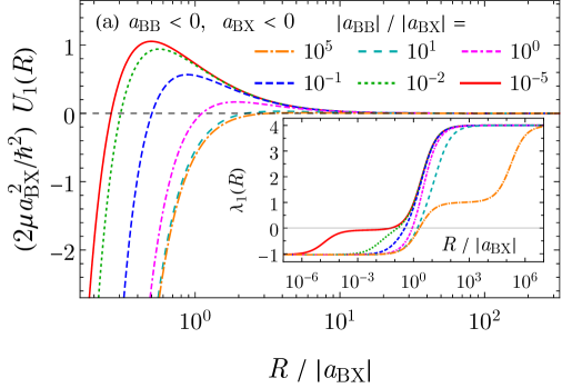
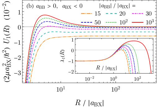
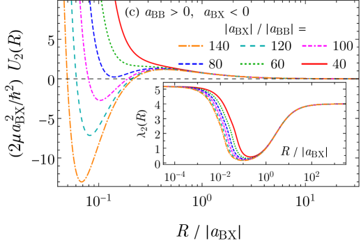
Figure 3: The zero-range hyperspherical potentials $U_{n}(R)$ for $a_{\text{BX}}<0$, shown for the lower (a and b) and upper (c) spectra. Curves within each panel correspond to different values of $|a_{\text{BB}}|/|a_{\text{BX}}|$. The insets show the corresponding hyperangular eigenvalues $\lambda_{n}(R)$.

Thus far, the Efimov spectrum has been examined only at $\absolutevalue{a_{\text{BX}}}\rightarrow\infty$. Generally, as $a_{\text{BX}}$ changes from $-\infty$ to $0$ with $a_{\text{BB}}$ fixed, Efimov states become less bound and eventually dissociate as the two-body interactions weaken in two pairs, leaving at most one pair resonant. This contrasts with the regime of Fig. 1, where Efimov states never become unbound for $a_{\text{BB}}<0$, since two pairs remain resonant while only one pair’s interaction weakens. Namely, the ZR potentials for $a_{\text{BX}}<0$, portrayed in Fig. 3, possess a shape barrier that is absent at unitarity (see Fig. 2). This barrier elevates Efimov states, initially residing in the unitarity potential, to the relevant dissociation threshold, where they become unbound at $a_{\text{BX}}=a_{-}^{(n)}$. Restated, at least two resonant pairs are required to sustain an Efimov trimer in heteronuclear systems.

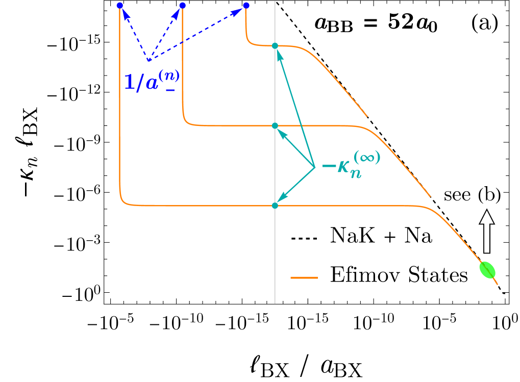
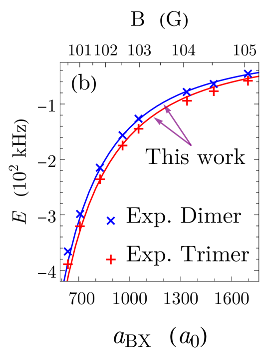
Figure 4: (a) The upper Efimov spectrum at $a_{\text{BB}}=52a_{0}$, computed from the FR model, shown vs. $1/a_{\text{BX}}$. (b) Zoomed-in view of the green-shaded area in (a), comparing the current work (solid) with experimental data [41].

For instance, in Fig. 4(a), the energies of the three resonances from Fig. 1 (upper right) are traced in $a_{\text{BX}}$, with $a_{\text{BB}}$ set to $52a_{0}$ [48, 49, 50]. Departing from unitarity in $a_{\text{BX}}$, the system exhibits typical Efimov behavior observed in homonuclear systems: Efimov states fade into the three-body continuum for $a_{\text{BX}}<0$ and merge with the dimer threshold for $a_{\text{BX}}>0$. Fig. 4(b) shows strong agreement between our FR model and the experimental energy of a recently detected $\ch{{}^{23}Na2^{40}K}$ halo trimer, indicated by the shaded area in Fig. 4(a), near a broad Na-K Feshbach resonance [41], thus providing a broader perspective on how the observed trimer fits within the usual Efimov scenario. Due to the large geometric spacing in the upper spectrum, the experimental regime for such a halo trimer ($a_{\text{BX}}\approx 30\,\ell_{\text{BX}}$) is too far from the Efimov domain in the present system ($a_{\text{BX}}\gtrsim 10^{6}\,\ell_{\text{BX}}$).

The unitarity (rescaled) energies $-\kappa_{n}^{(\infty)}$, studied in Fig. 1, and the values $a_{-}^{(n)}$, linked to resonances in the three-body loss rate, are indicated for the upper spectrum by solid and dashed arrows, respectively, in Fig. 4. The current system has two disparate Efimov spectra and therefore two sets of $a_{-}^{(n)}$ (and 3BPs) relevant for 3BR. This feature is exclusive to Efimov-unfavored systems, as increasing the mass ratio (toward Efimov-favored systems) causes the two spectra to smoothly merge into a single spectrum. Specifically, as $m_{\text{B}}/m_{\text{X}}\rightarrow\infty$, $s_{0}^{*}\leftrightarrow s_{0}$ and the two eigenvalues in the inset of Fig. 2(b) move closer to each other, becoming more strongly coupled.

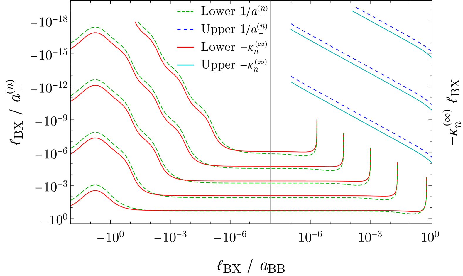
Figure 5: The Efimov resonances $a_{-}^{(n)}$ and the unitarity energies $-\kappa_{n}^{(\infty)}$, computed from the FR model, for the lower (green and red) and upper (blue and cyan) spectra. The presented quantities are relative to the three-body continuum, except for the lower spectrum when $a_{\text{BB}}>0$ (lower right), where $-\kappa_{n}^{(\infty)}$ (red) represent binding energies relative to the $\ch{Na2}$ dimer energy, and $a_{-}^{(n)}$ (green) indicate the values of $a_{\text{BX}}$ at which each Efimov state disappears into the atom-dimer continuum. The lower right curves were plot-truncated to avoid intersection with the upper curves.

Given the implied connection between $a_{-}^{(n)}$ and $-\kappa_{n}^{(\infty)}$ through the Efimov states [5], $a_{-}^{(n)}$ are expected to strongly depend on $a_{\text{BB}}$, similarly to the unitarity energies, as illustrated in Fig. 1. Using the FR model, $a_{-}^{(n)}$ were directly calculated over a range of $a_{\text{BB}}$ values by setting the total energy $E=0$. The dependence of $a_{-}^{(n)}$ on $a_{\text{BB}}$ is visualized in Fig. 5 for both the lower and upper spectra, with the unitarity energies $-\kappa_{n}^{(\infty)}$ overlaid to highlight the correlation. Manifestly, in Fig. 5, $1/a_{-}^{(n)}$ are generally correlated with $-\kappa_{n}^{(\infty)}$. Specifically, for $a_{\text{BB}}<0$, $1/a_{-}^{(n)}$ display the same oscillations and transition between two scaling factors as observed for the unitarity energies, leading to a significant variation in the Efimov resonance positions $a_{-}^{(n)}$ with $\absolutevalue{a_{\text{BB}}}$.

With $a_{\text{BB}}>0$, as $a_{\text{BX}}$ varies from $-\infty$ to $0$, the lower-spectrum states are blocked from reaching the three-body continuum by the $\ch{Na2}\,+\,\ch{K}$ threshold (i.e., they disappear into the atom-dimer continuum). It should be emphasized that for $a_{\text{BB}}>0$, the lower $a_{-}^{(n)}$ in Fig. 5 were computed with $E$ set to the $\ch{Na2}$ dimer energy instead of $E=0$. As a result, one should keep in mind that those lower $a_{-}^{(n)}$ would not show three-atom recombination resonances in a purely atomic gas, although there would be the possibility of recombination resonances in a mixed gas of dimers and atoms. Moreover, for $a_{\text{BB}}>0$, the first Efimov resonance $a_{-}^{(0)}$ becomes linked to the upper-spectrum ground state, which lies five orders of magnitude higher (in $-\kappa^{(\infty)}$) than the lower spectrum (see Fig. 1), thereby justifying the exceptionally large $|a_{-}^{(0)}|$ ($>10^{6}a_{0}$) reported by Wang et al. [31, 32] for $\ch{{}^{41}K2^{87}Rb}$ at $a_{\text{BB}}=62a_{0}$, consistent with the 3BP value inferred from Fig. 4. This suggests a considerably more observable 3BP value in Efimov-unfavored systems with negative $a_{\text{BB}}$, such as $\ch{{}^{85}Rb2^{133}Cs}$, where the value of $a_{\text{BB}}\approx-390a_{0}$ results in $a_{-}^{(0)}\approx-1800a_{0}$, which is achievable near the interspecies Feshbach resonances, for example, at $B\approx 107$ or $642$ G [51].

To summarize, we have identified two key mechanisms underlying the dramatic dependence of the Efimov resonance positions $a_{-}^{(n)}$ and the 3BP on the intraspecies scattering length $a_{\text{BB}}$ in Efimov-unfavored systems. For $a_{\text{BB}}<0$, the system undergoes a gradual transition between two markedly distinct Efimov scaling factors, resulting in a strong dependence of the Efimov spectrum on $\absolutevalue{a_{\text{BB}}}$. However, for $a_{\text{BB}}>0$, two qualitatively distinct Efimov spectra emerge above and below the homonuclear shallow dimer threshold. This leads to the association of the first Efimov resonance $a_{-}^{(0)}$ with the ground state of the upper spectrum, producing a 3BP of substantially large magnitude. Crucially, both mechanisms are driven by the large disparity between $s_{0}$ and $s_{0}^{*}$, a distinctive feature of Efimov-unfavored systems.

This work was supported by NSF grant No. 2207977.

Supplementary Material

.1 Three-Body Bound States

The pairwise two-body interactions are assumed to be described by separable potentials:

$$V_{i}(\vec{q},\vec{q}\,^{\prime})=\frac{\hbar^{2}}{2\mu_{i}}\alpha_{i}\ \chi_{i}(\vec{q}\,)\chi^{*}_{i}(\vec{q}\,^{\prime}),$$ (S.1)

for more on separable potentials see Ref. [1]. The three-body Schrödinger equation in momentum space, after eliminating the center of mass motion, reads

$$\left(\frac{\hbar^{2}p_{i}^{2}}{2\mu^{i}}+\frac{\hbar^{2}q_{i}^{2}}{2\mu_{i}}\right)\Psi(\vec{p}_{i},\vec{q}_{i})\;+\\ \sum_{j=1}^{3}\int\frac{d^{3}\vec{q}_{j}\!^{\prime}}{(2\pi)^{3}}V_{j}(\vec{q}_{j},\vec{q}_{j}\!^{\prime})\Psi(\vec{p}_{j},\vec{q}_{j}\!^{\prime})=E\,\Psi(\vec{p}_{i},\vec{q}_{i}),$$ (S.2)

where the Jacobi coordinate set $(\vec{p}_{i},\vec{q}_{i})$ is used to express the kinetic term while the relevant set $(\vec{p}_{j},\vec{q}_{j})$ is used for each of the three pairwise interaction terms. Inserting the separable potentials (Eq. (S.1)) in Eq. (S.2) gives

$$\left(\frac{p_{i}^{2}}{\mu^{i}}+\frac{q_{i}^{2}}{\mu_{i}}-\frac{2E}{\hbar^{2}}\right)\Psi(\vec{p}_{i},\vec{q}_{i})+\sum_{j=1}^{3}\chi_{j}(\vec{q}_{j})F_{j}(\vec{p}_{j})=0,$$ (S.3)

where the unknown functions $F_{i}(\vec{p}_{i})$ have been defined as

$$F_{i}(\vec{p}_{i})\equiv\frac{\alpha_{i}}{\mu_{i}}\int\frac{d^{3}\vec{q}_{i}}{(2\pi)^{3}}\chi^{*}_{i}(\vec{q}_{i})\Psi(\vec{p}_{i},\vec{q}_{i}).$$ (S.4)

Eq. (S.3) can be solved for $\Psi(\vec{p}_{i},\vec{q}_{i})$ as

$$\Psi(\vec{p}_{i},\vec{q}_{i})=-\sum_{j=1}^{3}\frac{\chi_{j}(\vec{q}_{j})F_{j}(\vec{p}_{j})}{\frac{p_{i}^{2}}{\mu^{i}}+\frac{q_{i}^{2}}{\mu_{i}}-\frac{2E}{\hbar^{2}}}.$$ (S.5)

Note that, since bound-state solutions ($E<0$) are of interest here, the right-hand side of Eq. (S.5) includes only a particular solution term and no homogeneous solution. By inserting Eq. (S.5) into Eq. (S.4), the following system of coupled integral equations is obtained

$$\left(\frac{\mu_{i}}{\alpha_{i}}+\int\frac{d^{3}\vec{q}_{i}}{(2\pi)^{3}}\frac{\absolutevalue{\chi_{i}(\vec{q}_{i})}^{2}}{\frac{p_{i}^{2}}{\mu^{i}}+\frac{q_{i}^{2}}{\mu_{i}}-\frac{2E}{\hbar^{2}}}\right)F_{i}(\vec{p}_{i})\;+\\ \sum_{j\neq i}\int\frac{d^{3}\vec{q}_{i}}{(2\pi)^{3}}\frac{\chi^{*}_{i}(\vec{q}_{i})\chi_{j}(\vec{q}_{j})}{\frac{p_{i}^{2}}{\mu^{i}}+\frac{q_{i}^{2}}{\mu_{i}}-\frac{2E}{\hbar^{2}}}F_{j}(\vec{p}_{j})=0,$$ (S.6)

where the $j=i$ term has been factored out of the sum. Now, this system is not readily solvable numerically since the argument of $F_{j}(\vec{p}_{j})$ is not identical with the integration variable $\vec{q}_{i}$, which is essential for recasting the integral operator as a matrix multiplication. To this purpose, the following relations are used to write the Jacobi set $(\vec{p}_{j},\vec{q}_{j})$ in terms of $(\vec{p}_{i},\vec{q}_{i})$

$$\vec{p}_{j} =\frac{-m_{j}}{m_{j}+m_{k}}\,\vec{p}_{i}\;+\;\epsilon_{ij}\,\vec{q}_{i}$$ (S.7)

$$\vec{q}_{j} =\epsilon_{ji}\frac{m_{k}M}{(m_{i}+m_{k})(m_{j}+m_{k})}\,\vec{p}_{i}\;+\;\frac{-m_{i}}{m_{i}+m_{k}}\,\vec{q}_{i},$$

where $\epsilon_{ij}$ is the Levi-Civita symbol, $M$ is the total mass, and $k=6-i-j$. Upon plugging these expressions into Eq. (S.6) and redefining the integration variable as $\vec{q}_{i}\rightarrow\epsilon_{ij}\left(\vec{q}_{i}+\frac{m_{j}}{m_{j}+m_{k}}\,\vec{p}_{i}\right)$, one gets

$$\left(\frac{\mu_{i}}{\alpha_{i}}+\int\frac{d^{3}\vec{q}}{(2\pi)^{3}}\frac{\absolutevalue{\chi_{i}(\vec{q}\,)}^{2}}{\frac{p^{2}}{\mu^{i}}+\frac{q^{2}}{\mu_{i}}-\frac{2E}{\hbar^{2}}}\right)F_{i}(\vec{p}\,)\;+\sum_{j\neq i}\\ \int\frac{d^{3}\vec{q}}{(2\pi)^{3}}\frac{\chi^{*}_{i}\!\left(\epsilon_{ij}\left[\vec{q}+\frac{m_{j}}{m_{j}+m_{k}}\vec{p}\,\right]\right)\chi_{j}\!\left(\epsilon_{ji}\left[\vec{p}+\frac{m_{i}}{m_{i}+m_{k}}\vec{q}\,\right]\right)}{\frac{p^{2}}{\mu_{j}}+\frac{q^{2}}{\mu_{i}}+\frac{2}{m_{k}}\vec{p}\cdot\vec{q}-\frac{2E}{\hbar^{2}}}\\ \times F_{j}(\vec{q}\,)=0,$$ (S.8)

where the indices on the momentum coordinates $(\vec{p},\vec{q}\,)$ have been omitted.

Thus far, no presumptions have been made on the interaction form factors $\chi_{i}(\vec{q}\,)$. Moving forward, $s$-wave interactions are assumed among the three particles, i.e., $\chi_{i}(\vec{q}\,)=\chi_{i}(q)$. Following Naidon, Endo, and Ueda [2], our treatment adopts the following form factor that models van der Waals pairwise interactions

$$\chi_{i}(q)=1-q\int_{0}^{\infty}\left(1-\frac{r}{a_{i}}-\varphi_{i}(r)\right)\sin(qr)\,dr,$$ (S.9)

and the prefactor $\alpha_{i}$ is selected as

$$\frac{1}{\alpha_{i}}=\frac{1}{4\pi a_{i}}-\frac{1}{2\pi^{2}}\int_{0}^{\infty}dq\absolutevalue{\chi_{i}(q)}^{2},$$ (S.10)

where $a_{i}$ are the $s$-wave scattering lengths and $\varphi(r)$ is the zero-energy $s$-wave radial solution of the van der Waals potential in the two-body sector. This form factor choice is shown to reproduce the low-energy features of the full potential, such as the scattering length and the high-lying dimer bound state. In particular, it gives the exact solution of the two-body Schrödinger equation at zero energy, namely $\varphi(r)$. For three-body states with total angular momentum $L$, the angular dependence of $F_{i}(\vec{p}\,)$ is given by $F_{i}(p)\,Y_{LM}(\hat{p})$.

Utilization of the previous facts and Eq. (S.10) reduces Eq. (S.8) to a one-dimensional system of coupled integral equations

$$D_{i}(p)F_{i}(p)+\sum_{j\neq i}\int_{0}^{\infty}H_{ij}(p,q)F_{j}(q)\,dq=0,$$ (S.11)

with

$$D_{i}(p)=\mu_{i}\left(\frac{\pi}{a_{i}}-2\left(\frac{p^{2}}{\mu^{i}}-\frac{2E}{\hbar^{2}}\right)\int_{0}^{\infty}\frac{\absolutevalue{\chi_{i}(q)}^{2}dq}{\frac{q^{2}}{\mu_{i}}+\frac{p^{2}}{\mu^{i}}-\frac{2E}{\hbar^{2}}}\right),$$ (S.12)

$$H_{ij}(p,q)=\int_{-1}^{1}du\,P_{L}(u)\,q^{2}\\ \times\frac{\chi^{*}_{i}\!\left(\absolutevalue{\vec{q}+\frac{m_{j}}{m_{j}+m_{k}}\vec{p}\,}\right)\chi_{j}\!\left(\absolutevalue{\vec{p}+\frac{m_{i}}{m_{i}+m_{k}}\vec{q}\,}\right)}{\frac{p^{2}}{\mu_{j}}+\frac{q^{2}}{\mu_{i}}+\frac{2}{m_{k}}pqu-\frac{2E}{\hbar^{2}}},$$ (S.13)

where $P_{L}(u)$ is a Legendre polynomial. After discretizing the linear operators of Eqs. (S.11), one can solve for the three-body bound state energy $E$ by searching for roots of the resulting determinantal equation. Stated differently, Eqs. (S.11) can be recast as a $3\times 3$ block matrix operator acting on a vector of unknown functions $F_{i}$ as follows:

$$\begin{pmatrix}D_{1}&H_{12}&H_{13}\\ H_{21}&D_{2}&H_{23}\\ H_{31}&H_{32}&D_{3}\end{pmatrix}\begin{pmatrix}F_{1}\\ F_{2}\\ F_{3}\end{pmatrix}=0,$$ (S.14)

where the multiplication between each element of the block matrix and the functions $F_{i}$ is understood as a matrix product in momentum space. Hence, by seeking the special energy values at which one of the eigenvalues (and the determinant) of the block matrix in Eq. (S.14) vanishes, the allowed trimer state energies are determined for any three $s$-wave scattering lengths $a_{i}$, three masses $m_{i}$, and a given total angular momentum $L$.

Note that instead of searching for roots in energy $E$ at a fixed set of scattering lengths $a_{i}$, one can search for roots in scattering lengths at a given energy. For example, this approach proves useful in solving for $a_{-}^{(n)}$ in either homonuclear or heteronuclear systems by solving the determinantal equation at the three-body threshold ($E=0$).

.2 Imposing Particles Symmetry

In this subsection, the symmetry constraints are derived for systems with arbitrary exchange symmetry (i.e., some or all of the three particles are identical bosons/fermions). These constraints, which will ultimately impose conditions on the unknowns $F_{i}(p)$, simplify the system in Eqs. (S.11) by reducing the total number of equations and unknowns.

The starting point is the fact that permuting the relevant bosons (fermions), along with their intrinsic degrees of freedom, should not affect (or should introduce a minus sign to) the properly symmetrized (antisymmetrized) three-body wavefunction. For example, if particle 1 and 2 are identical bosons, permuting their momenta ($\vec{k}_{1}$ and $\vec{k}_{2}$) should leave the wavefunction unchanged. Given that $\hat{P}_{12}(\vec{p}_{1},\vec{q}_{1})=(\vec{p}_{2},-\vec{q}_{2})$ and $\hat{P}_{12}(\vec{p}_{3},\vec{q}_{3})=(\vec{p}_{3},-\vec{q}_{3})$, Eq. (S.5) implies that

$$\chi_{1}(\vec{q}_{1})F_{1}(\vec{p}_{1})+\chi_{2}(\vec{q}_{2})F_{2}(\vec{p}_{2})+\chi_{3}(\vec{q}_{3})F_{3}(\vec{p}_{3})=$$

$$\chi_{1}(-\vec{q}_{2})F_{1}(\vec{p}_{2})+\chi_{2}(-\vec{q}_{1})F_{2}(\vec{p}_{1})+\chi_{3}(-\vec{q}_{3})F_{3}(\vec{p}_{3})=$$

$$\chi_{2}(\vec{q}_{2})F_{1}(\vec{p}_{2})+\chi_{1}(\vec{q}_{1})F_{2}(\vec{p}_{1})+\chi_{3}(\vec{q}_{3})F_{3}(\vec{p}_{3})$$ (S.15)

where the property of $s$-wave interactions $\chi_{i}(-\vec{q}\,)=\chi_{i}(\vec{q}\,)$ and the fact that $\chi_{1}=\chi_{2}$, which follows immediately from particle 1 and 2 being identical, have been used in the last equality. Comparing the first and last lines of Eq. (.2), leads to the conclusion that $F_{2}=F_{1}$ and no restriction on $F_{3}$, simplifying the original coupled system in Eqs. (S.11) to two equations in two unknowns $F_{1}(p)$ and $F_{3}(p)$. Similarly, if particles 1 and 2 are fermions, one could show that the required symmetry constraints are $F_{2}=-F_{1}$ and $F_{3}=0$. The vanishing of $F_{3}$ in this case merely reflects the fact that fermions cannot interact via $s$-wave interactions. However, if a $p$-wave interaction is allowed between only the two fermions, i.e., $\chi_{3}(-\vec{q}_{3})=-\chi_{3}(\vec{q}_{3})$, one finds that $F_{3}\neq 0$. The required exchange symmetry constraints on $F_{i}$ for different systems are summarized in Table S.I.

XXX	$F_{1}$	$F_{2}$	$F_{3}$
BBX	$F_{1}$	$F_{1}$	$F_{3}$
FFX	$F_{1}$	$-F_{1}$	$0$
BBB	$F_{1}$	$F_{1}$	$F_{1}$

Table S.I: The necessary symmetry conditions are provided for three-body systems with different particle exchange symmetries (assuming $s$-wave interactions), where X denotes a distinguishable particle, B an identical boson, and F an identical fermion.

.3 The Unitarity Spectrum

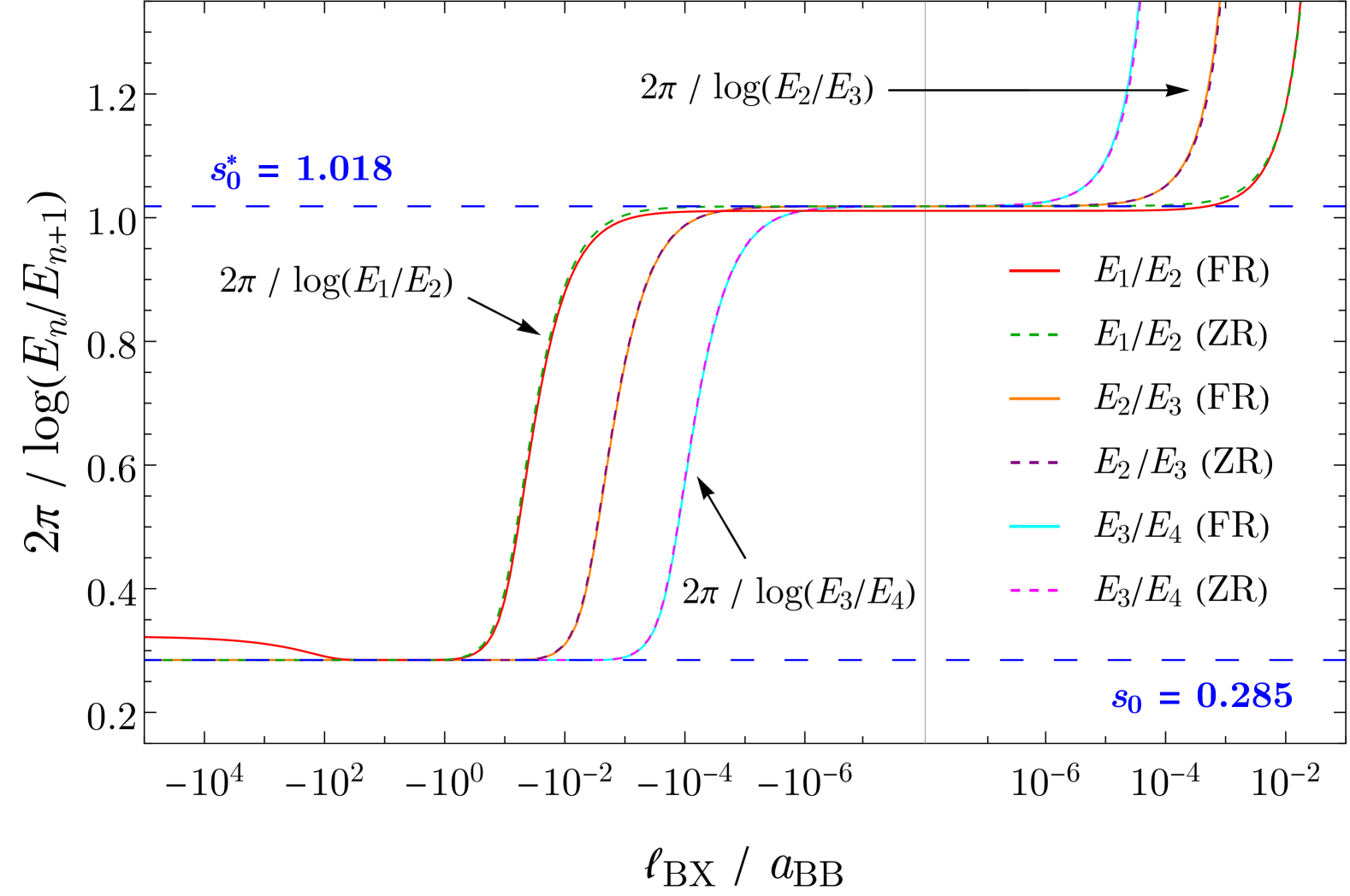
Figure S.1: The variable Efimov scaling parameter, given through the ratios $E_{n}/E_{n+1}$ at $\absolutevalue{a_{\text{BX}}}\rightarrow\infty$, graphed for the lowest three pairs of consecutive trimer states depicted in Fig. 1 of the main article. Solid curves correspond to finite-range calculations, while dashed curves correspond to zero-range calculations. The horizontal dashed blue lines represent the universal Efimov scaling parameters: $s_{0}^{*}=1.018$ (upper) at $1/a_{\text{BB}}=0$ and $s_{0}=0.285$ (lower) at $1/a_{\text{BB}}\rightarrow-\infty$, which correspond to three and two resonant pairs respectively.

The variation of the Efimov scaling factor in the lower spectrum, produced by the interplay between the transition region and the bound states’ turning points as $a_{\text{BB}}$ changes from $-\infty$ to $0$, is summarized in Fig. S.1, which involve Efimov ratios calculated from the unitarity energy spectrum.

Note that the lower trimers do not extend above the $\ch{Na2}\,+\,\ch{K}$ threshold in Fig. 1 of the main article, a behavior supported by analyzing the atom-dimer scattering length $a_{\text{AD}}$. Fig. S.2 reveals that $a_{\text{AD}}$ (solid) changes from $\infty$ to $-\infty$ periodically at specific $a_{\text{BB}}$ values that align neatly with the values (dashed) where the lower spectrum loses a bound state for $a_{\text{BB}}>0$ (i.e., trimer-dimer intersections), signifying the possibility of the Efimov effect in an ultracold gas of $\ch{Na2}$ dimers and $\ch{K}$ atoms.

Figure S.2: The atom-dimer ($\ch{K}-\ch{Na2}$) scattering length $a_{\text{AD}}$ at $\absolutevalue{a_{\text{BX}}}\rightarrow\infty$, calculated from the zero-range potential $U_{1}(R)$ for $a_{\text{BB}}>0$ associated with the lower spectrum (see Fig. 2(b) of the main article). The vertical dashed lines mark the values of $a_{\text{BB}}$ at which the lower spectrum trimers intersect the $\ch{Na2}\,+\,\ch{K}$ threshold, as determined from the ZR data in Fig. 1 of the main article. Recall that this ZR calculation is equipped with a log-derivative that ties it with the FR model.

To obtain the upper resonances as solutions of Eqs. (S.11) (i.e., the finite-range model), originally developed for true bound states, the discrete momentum mesh (i.e., the values $(p,q)$ used to tabulate the matrix in Eq. (S.14)) must be adjusted to exclude the degenerate continuum states of the lower channel, $\ch{Na2}\,+\,\ch{K}$. This momentum-space projection onto the upper channel subspace is equivalent to the real-space projection, where bound states are sought exclusively in the upper potential $U_{2}(R)$, ignoring nonadiabatic couplings to other channels.

.4 The Efimov Resonances

Valuable insight into the behavior of $a_{-}^{(n)}$ (e.g., their connection with $\kappa_{n}^{(\infty)}$) can be gained by investigating the relevant ZR potential curves. In contrast to the unitarity potentials, the potentials for $a_{\text{BX}}<0$ feature a shape barrier located on average at $R_{b}\sim\absolutevalue{a_{\text{BX}}}$, as shown in Fig. 3 of the main article. As this barrier moves inward (i.e., as $\absolutevalue{a_{\text{BX}}}$ decreases), it overlaps with an Efimov state (initially residing in a unitarity potential curve), elevating the state to the relevant continuum threshold, upon which it dissociates at $a_{\text{BX}}=a_{-}^{(n)}$. This overlap occurs when the barrier position becomes comparable to the state’s turning point at unitarity ($R_{b}\sim R_{t}$), leading to $|1/a_{-}^{(n)}|\sim\kappa_{n}^{(\infty)}$, thereby justifying the correlation with the unitarity energies.

However, $1/a_{-}^{(n)}$ do not precisely track the unitarity energies, i.e., the ratio $|1/a_{-}^{(n)}|/\kappa_{n}^{(\infty)}$ is not constant in different regions of Fig. 5 of the main article. For instance, $|1/a_{-}^{(n)}|>\kappa_{n}^{(\infty)}$ near $\absolutevalue{a_{\text{BB}}}\rightarrow\infty$, while $|1/a_{-}^{(n)}|<\kappa_{n}^{(\infty)}$ as $a_{\text{BB}}\rightarrow 0^{-}$. This variable ratio $|1/a_{-}^{(n)}|/\kappa_{n}^{(\infty)}$ for $a_{\text{BB}}<0$ can be explained by scrutinizing Fig. 3(a) of the main article, which reveals that the barrier’s position and shape (width and height) hinge on the ratio $\absolutevalue{a_{\text{BB}}}/\absolutevalue{a_{\text{BX}}}$. The barrier occurs later than $\absolutevalue{a_{\text{BX}}}$ ($R_{b}>\absolutevalue{a_{\text{BX}}}$) if $\absolutevalue{a_{\text{BB}}}>\absolutevalue{a_{\text{BX}}}$ (e.g., orange and cyan), while it occurs earlier than $\absolutevalue{a_{\text{BX}}}$ ($R_{b}<\absolutevalue{a_{\text{BX}}}$) if $\absolutevalue{a_{\text{BB}}}<\absolutevalue{a_{\text{BX}}}$ (e.g., red and green). This results in $|1/a_{-}^{(n)}|>\kappa_{n}^{(\infty)}$ below the curve $y=-\absolutevalue{x}$ ($\absolutevalue{a_{\text{BX}}}=\absolutevalue{a_{\text{BB}}}$), and $|1/a_{-}^{(n)}|<\kappa_{n}^{(\infty)}$ above it, as evident in Fig. 5 of the main article. This reasoning is supported by observing that the red and green curves in Fig. 5 of the main article intersect (i.e., $|1/a_{-}^{(n)}|=\kappa_{n}^{(\infty)}$) near $\absolutevalue{a_{\text{BB}}}=\absolutevalue{a_{\text{BX}}}$, marking a transition point for the ratio $|1/a_{-}^{(n)}|/\kappa_{n}^{(\infty)}$. For $\absolutevalue{a_{\text{BB}}}>0$, the barrier lies on opposite sides of $\absolutevalue{a_{\text{BX}}}$ for the lower and upper spectra, i.e., see Figs. 3(b–c) of the main article. Hence, the two spectra lie on opposite sides of unity in this ratio, i.e., $|1/a_{-}^{(n)}|/\kappa_{n}^{(\infty)}>1$ for the lower spectrum and vice versa.

References

- Chin et al. [2010] C. Chin, R. Grimm, P. Julienne, and E. Tiesinga, Rev. Mod. Phys. 82, 1225 (2010).
- Bartenstein et al. [2005] M. Bartenstein, A. Altmeyer, S. Riedl, R. Geursen, S. Jochim, C. Chin, J. H. Denschlag, R. Grimm, A. Simoni, E. Tiesinga, C. J. Williams, and P. S. Julienne, Phys. Rev. Lett. 94, 103201 (2005).
- Efimov [1970] V. Efimov, Physics Letters B 33, 563 (1970).
- Petrov [2004] D. S. Petrov, Phys. Rev. Lett. 93, 143201 (2004).
- Braaten and Hammer [2006] E. Braaten and H.-W. Hammer, Physics Reports 428, 259 (2006).
- Hammer and Platter [2007] H.-W. Hammer and L. Platter, The European Physical Journal A 32, 113 (2007).
- von Stecher et al. [2009] J. von Stecher, J. P. D’Incao, and C. H. Greene, Nature Physics 5, 417 (2009).
- Wang and Esry [2009] Y. Wang and B. D. Esry, Phys. Rev. Lett. 102, 133201 (2009).
- Zenesini et al. [2013] A. Zenesini, B. Huang, M. Berninger, S. Besler, H.-C. Nägerl, F. Ferlaino, R. Grimm, C. H. Greene, and J. von Stecher, New Journal of Physics 15, 043040 (2013).
- Naidon and Endo [2017] P. Naidon and S. Endo, Reports on Progress in Physics 80, 056001 (2017).
- Greene et al. [2017] C. H. Greene, P. Giannakeas, and J. Pérez-Ríos, Rev. Mod. Phys. 89, 035006 (2017).
- Kraemer et al. [2006] T. Kraemer, M. Mark, P. Waldburger, J. G. Danzl, C. Chin, B. Engeser, A. D. Lange, K. Pilch, A. Jaakkola, H.-C. Nägerl, and R. Grimm, Nature 440, 315 (2006).
- Knoop et al. [2009] S. Knoop, F. Ferlaino, M. Mark, M. Berninger, H. Schöbel, H.-C. Nägerl, and R. Grimm, Nature Physics 5, 227 (2009).
- Berninger et al. [2011] M. Berninger, A. Zenesini, B. Huang, W. Harm, H.-C. Nägerl, F. Ferlaino, R. Grimm, P. S. Julienne, and J. M. Hutson, Phys. Rev. Lett. 107, 120401 (2011).
- Huang et al. [2014] B. Huang, L. A. Sidorenkov, R. Grimm, and J. M. Hutson, Phys. Rev. Lett. 112, 190401 (2014).
- Wild et al. [2012] R. J. Wild, P. Makotyn, J. M. Pino, E. A. Cornell, and D. S. Jin, Phys. Rev. Lett. 108, 145305 (2012).
- Zaccanti et al. [2009] M. Zaccanti, B. Deissler, C. D’Errico, M. Fattori, M. Jona-Lasinio, S. Müller, G. Roati, M. Inguscio, and G. Modugno, Nature Physics 5, 586 (2009).
- Pollack et al. [2009] S. E. Pollack, D. Dries, and R. G. Hulet, Science 326, 1683 (2009).
- Gross et al. [2009] N. Gross, Z. Shotan, S. Kokkelmans, and L. Khaykovich, Phys. Rev. Lett. 103, 163202 (2009).
- Ottenstein et al. [2008] T. B. Ottenstein, T. Lompe, M. Kohnen, A. N. Wenz, and S. Jochim, Phys. Rev. Lett. 101, 203202 (2008).
- Huckans et al. [2009] J. H. Huckans, J. R. Williams, E. L. Hazlett, R. W. Stites, and K. M. O’Hara, Phys. Rev. Lett. 102, 165302 (2009).
- Wenz et al. [2009] A. N. Wenz, T. Lompe, T. B. Ottenstein, F. Serwane, G. Zürn, and S. Jochim, Phys. Rev. A 80, 040702 (2009).
- Williams et al. [2009] J. R. Williams, E. L. Hazlett, J. H. Huckans, R. W. Stites, Y. Zhang, and K. M. O’Hara, Phys. Rev. Lett. 103, 130404 (2009).
- Lompe et al. [2010] T. Lompe, T. B. Ottenstein, F. Serwane, K. Viering, A. N. Wenz, G. Zürn, and S. Jochim, Phys. Rev. Lett. 105, 103201 (2010).
- Nakajima et al. [2010] S. Nakajima, M. Horikoshi, T. Mukaiyama, P. Naidon, and M. Ueda, Phys. Rev. Lett. 105, 023201 (2010).
- Ferlaino et al. [2009] F. Ferlaino, S. Knoop, M. Berninger, W. Harm, J. P. D’Incao, H.-C. Nägerl, and R. Grimm, Phys. Rev. Lett. 102, 140401 (2009).
- Esry et al. [1999] B. D. Esry, C. H. Greene, and J. P. Burke, Phys. Rev. Lett. 83, 1751 (1999).
- Efimov [1973] V. Efimov, Nuclear Physics A 210, 157 (1973).
- D’Incao and Esry [2006] J. P. D’Incao and B. D. Esry, Phys. Rev. A 73, 030702 (2006).
- Helfrich et al. [2010] K. Helfrich, H.-W. Hammer, and D. S. Petrov, Phys. Rev. A 81, 042715 (2010).
- Wang et al. [2012] Y. Wang, J. Wang, J. P. D’Incao, and C. H. Greene, Phys. Rev. Lett. 109, 243201 (2012).
- Wang et al. [2015] Y. Wang, J. Wang, J. P. D’Incao, and C. H. Greene, Phys. Rev. Lett. 115, 069901 (2015).
- Petrov and Werner [2015] D. S. Petrov and F. Werner, Phys. Rev. A 92, 022704 (2015).
- Barontini et al. [2009] G. Barontini, C. Weber, F. Rabatti, J. Catani, G. Thalhammer, M. Inguscio, and F. Minardi, Phys. Rev. Lett. 103, 043201 (2009).
- Wacker et al. [2016] L. J. Wacker, N. B. Jørgensen, D. Birkmose, N. Winter, M. Mikkelsen, J. Sherson, N. Zinner, and J. J. Arlt, Phys. Rev. Lett. 117, 163201 (2016).
- Maier et al. [2015] R. A. W. Maier, M. Eisele, E. Tiemann, and C. Zimmermann, Phys. Rev. Lett. 115, 043201 (2015).
- Tung et al. [2014] S.-K. Tung, K. Jiménez-García, J. Johansen, C. V. Parker, and C. Chin, Phys. Rev. Lett. 113, 240402 (2014).
- Ulmanis et al. [2016a] J. Ulmanis, S. Häfner, R. Pires, F. Werner, D. S. Petrov, E. D. Kuhnle, and M. Weidemüller, Phys. Rev. A 93, 022707 (2016a).
- Ulmanis et al. [2016b] J. Ulmanis, S. Häfner, R. Pires, E. D. Kuhnle, Y. Wang, C. H. Greene, and M. Weidemüller, Phys. Rev. Lett. 117, 153201 (2016b).
- Häfner et al. [2017] S. Häfner, J. Ulmanis, E. D. Kuhnle, Y. Wang, C. H. Greene, and M. Weidemüller, Phys. Rev. A 95, 062708 (2017).
- Chuang et al. [2024] A. Y. Chuang, H. Q. Bui, A. Christianen, Y. Zhang, Y. Ni, D. Ahmed-Braun, C. Robens, and M. W. Zwierlein, Observation of a halo trimer in an ultracold bose-fermi mixture (2024), arXiv:2411.04820 [cond-mat.quant-gas] .
- Yamaguchi [1954] Y. Yamaguchi, Phys. Rev. 95, 1628 (1954).
- Naidon et al. [2014] P. Naidon, S. Endo, and M. Ueda, Phys. Rev. A 90, 022106 (2014).
- [44] See Supplemental Material (next page) for a derivation of Eqs. 5 as well as additional insights into the behavior of the Efimov spectrum.
- Arora and Sahoo [2014] B. Arora and B. K. Sahoo, Phys. Rev. A 89, 022511 (2014).
- Mitroy and Bromley [2003] J. Mitroy and M. W. J. Bromley, Phys. Rev. A 68, 052714 (2003).
- Rittenhouse et al. [2010] S. T. Rittenhouse, N. P. Mehta, and C. H. Greene, Phys. Rev. A 82, 022706 (2010).
- Gutierrez et al. [2021] E. M. Gutierrez, G. A. de Oliveira, K. M. Farias, V. S. Bagnato, and P. C. M. Castilho, Applied Sciences 11, 10.3390/app11199099 (2021).
- Schulze et al. [2018] T. A. Schulze, T. Hartmann, K. K. Voges, M. W. Gempel, E. Tiemann, A. Zenesini, and S. Ospelkaus, Phys. Rev. A 97, 023623 (2018).
- Tiesinga et al. [1996] E. Tiesinga, C. J. Williams, P. S. Julienne, K. M. Jones, P. D. Lett, and W. D. Phillips, J Res Natl Inst Stand Technol 101, 505 (1996).
- Cui et al. [2018] Y. Cui, M. Deng, L. You, B. Gao, and M. K. Tey, Phys. Rev. A 98, 042708 (2018).

References

- Yamaguchi [1954] Y. Yamaguchi, Phys. Rev. 95, 1628 (1954).
- Naidon et al. [2014] P. Naidon, S. Endo, and M. Ueda, Phys. Rev. A 90, 022106 (2014).