Knowledge-guided machine learning model with soil moisture for corn yield prediction under drought conditions
Abstract
Remote sensing (RS) techniques, by enabling non-contact acquisition of extensive ground observations, have become a valuable tool for corn yield prediction. Traditional process-based (PB) models are limited by fixed input features and struggle to incorporate large volumes of RS data. In contrast, machine learning (ML) models are often criticized for being “black boxes” with limited interpretability. To address these limitations, we used Knowledge-Guided Machine Learning (KGML), which combined the strengths of both approaches and fully used RS data. However, previous KGML methods overlooked the crucial role of soil moisture in plant growth. To bridge this gap, we proposed the Knowledge-Guided Machine Learning with Soil Moisture (KGML-SM) framework, using soil moisture as an intermediate variable to emphasize its key role in plant development. Additionally, based on the prior knowledge that the model may overestimate under drought conditions, we designed a drought-aware loss function that penalizes predicted yield in drought-affected areas. Our experiments showed that the KGML-SM model outperformed other ML models. Finally, we explored the relationships between drought, soil moisture, and corn yield prediction, assessing the importance of various features and analyzing how soil moisture impacts corn yield predictions across different regions and time periods.
keywords:
Corn yield prediction; Knowledge-guided Machine learning; Soil moisture; drought[inst1]organization=Biological Systems Engineering,addressline=University of Wisconsin-Madison, city=Madison, postcode=53706, state=WI, country=USA
[inst2]organization=Department of of Soil Science,addressline=University of Wisconsin-Madison, city=Madison, postcode=53706, state=WI, country=USA
[inst3]organization=Research and Development Division, National Agricultural Statistics Service, United States Department of Agriculture,addressline=Washington, postcode=20250, state=DC, country=USA
1 Introduction
Corn plays a vital place in the U.S. as a primary crop, supporting food security as well as the animal feed and biofuel industries (Graham et al., 2007; Thompson, 1969). Accurate yield prediction is crucial for effective resource management and economic stability (Kucharik and Ramankutty, 2005). However, achieving precise prediction across large areas and diverse environmental conditions is challenging, making it necessary to pursue advanced research in corn yield prediction techniques (Weiss et al., 2020). Traditional process-based (PB) models (Weiss et al., 2007) are built on a deep understanding of the physical, chemical, and biological processes within crop growth systems (Weiss et al., 2004). These models use equations derived from scientific principles to simulate the behavior of crops, weather, and soil interactions (Weiss et al., 2002), making them highly interpretable and reliable in scenarios where the underlying processes are well understood (Puntel et al., 2016; Shahhosseini et al., 2021). Several promising modeling frameworks are designed for simulating and predicting agricultural production systems, such as The Agricultural Production Systems sIMulator (APSIM) (McCown et al., 1996), Decision Support System for Agrotechnology Transfer (DSSAT) (Jones et al., 2003), WOrld FOod STudies (WOFOST) (Van Diepen et al., 1989), and The Agricultural Policy / Environmental eXtender (APEX) (Williams and Izaurralde, 2010). Many recent studies (Zhen et al., 2023, 2022) have successfully used these models to predict crop yields. However, PB models have several limitations. Plant growth is highly complex, and these models rely on a limited set of fixed input features, which are insufficient to accurately capture the intricacies of this process. Moreover, PB models require extensive manual parameter tuning, limiting their applicability for large-scale applications across vast regions.
In recent years, remote sensing (RS) has provided several benefits for corn yield prediction (Lobell et al., 2015). It allows for the collection of large-scale and real-time data across vast agricultural areas, which, in conjunction with machine learning (ML) methods, provides an accurate and efficient way for large-scale yield prediction. Deep learning (Goodfellow et al., 2016), a widely used ML method, has the advantage of leveraging vast amounts of RS data by automatically learning features from large datasets. This removes the need for manual feature engineering, enabling the model to capture complex patterns and relationships between environmental factors and crop yield (He et al., 2016). Many studies have applied deep learning to crop yield prediction and shown its advantages. You et al. (2017) introduced a scalable approach to crop yield prediction using modern representation learning rather than traditional hand-crafted features, achieving impressive results. Wang et al. (2018) demonstrated soybean yield predictions in Argentina and obtained reliable results in Brazil using transfer learning, even with limited data. Ma et al. (2021a) developed a county-level corn yield prediction model using a Bayesian Neural Network across 12 states in the Corn Belt, showing the potential for large-scale corn yield prediction tasks. However, despite the popularity of deep learning models in corn yield prediction tasks, they have certain limitations. First, deep learning models require a large amount of data to learn the relationships between inputs and outputs. Second, deep learning models often function as a black box, lacking reliable interpretability of the prediction results. Therefore, finding ways to expand our data sources is a critical factor in achieving accurate predictions. Additionally, there are complex biological processes among soil, weather, and corn, which are challenging for deep learning models to fully capture. Given these challenges, combining PB models with deep learning models has become an important research topic.
Knowledge-guided machine learning (KGML) (Karpatne et al., 2022) aims to integrate scientific knowledge in ML frameworks to achieve better generalizability, scientific consistency, and explainability of results. KGML involves three main approaches: Knowledge-Guided Learning, Knowledge-Guided Architecture, and Knowledge-Guided Pretraining. Knowledge-Guided Learning incorporates scientific knowledge, such as physical laws, into the learning algorithm by modifying the loss function. It guides the optimization process toward scientifically consistent and generalizable solutions (Daw et al., 2022; Bao et al., 2021). Knowledge-Guided Architecture embeds scientific knowledge directly into the structure of the ML model. By designing knowledge-guided neural network architectures, researchers can enable models to automatically capture physical properties or conservation laws, which improves both interpretability and robustness (Dugdale et al., 2017; Luo et al., 2023). Knowledge-Guided Pretraining uses simulated data or self-supervised learning tasks to pretrain ML models. By initializing model parameters using data that encodes scientific principles, this method reduces the need for large amounts of observational data and improves performance in data-scarce scenarios (Licheng et al., 2022; Chen et al., 2023). Building on these approaches, KGML has been increasingly applied in various domains, including agriculture, hydrology, and climate science, enabling improved data-driven decision-making and predictive modeling.
Recently, many studies have used KGML to combine PB models and ML models for crop yield prediction (Kimball et al., 2023; Burroughs et al., 2023). Since PB models already provide insights into the crop growth process and generate high-quality simulated data, Knowledge-Guided Pretraining is the most popular approach (He et al., 2023; Yang et al., 2023). These studies aim to use ML to identify patterns between crop features and yield from large datasets, while also deriving interpretability from the data simulated by PB models. Specifically, KGML models leverage PB models to simulate intermediate variables representing key plant growth processes, enhancing their ability to capture domain-specific knowledge. Then, ML models are applied to simulate specific parts of the process. By incorporating these intermediate variables, the model can better represent the underlying biological and environmental mechanisms. For example, He et al. (2023) integrated physical knowledge from PB models and enabled the model to adjust for temporal data shifts over the years. Yang et al. (2023) used both historical and in-season RS data to better predict key agricultural variables such as grain yield and carbon cycling processes. Yang et al. (2024) presented a knowledge-guided computer vision framework designed to monitor and simulate the growth of individual strawberry fruits, which can predict growth at the individual fruit level by integrating image-based data and dynamic simulations.
Although these KGML models have made significant progress in crop yield prediction, all existing KGML-based studies on crop yield prediction have overlooked the critical role of soil, particularly how soil moisture contributes to plant growth and affects yield. Soil moisture is influenced by temperature, precipitation, and other environmental factors and directly affects crop growth. Unlike RS data, soil moisture has a cumulative impact on yield over time. As a key drought indicator, low soil moisture causes water stress, which limits corn growth and reduces yields (Unganai and Kogan, 1998). Nonetheless, both PB and ML models have certain limitations in modeling soil moisture. In PB models, weather data serve as input, while soil moisture is treated as output (McCown et al., 1996; Williams and Izaurralde, 2010), failing to capture its direct impact on crop yield. In ML models, a key challenge is the limited soil moisture data. For example, as the most commonly used soil moisture dataset, the SPL4SMGP.007 SMAP dataset (Entekhabi et al., 2010) only covers data from 2015 onward, limiting ML models’ ability to learn from extensive historical data and impacting the model performance. Therefore, we integrated PB and ML models through KGML to better model soil moisture for corn yield prediction. Additionally, we examined how soil moisture variations over time and across space affected corn yield in drought-prone areas, where drought often reduced yields and hindered prediction accuracy (Cooper et al., 2014). Researchers have long been interested in studying the relationship between soil moisture, drought, and corn yield prediction (Ines et al., 2013; Bushong et al., 2016; Mladenova et al., 2017). However, these studies either have a narrow scope (Vergopolan et al., 2021), resulting in limited data that cannot be effectively generalized to broader applications, or they focus solely on end-of-season yield prediction (Pignotti et al., 2023).
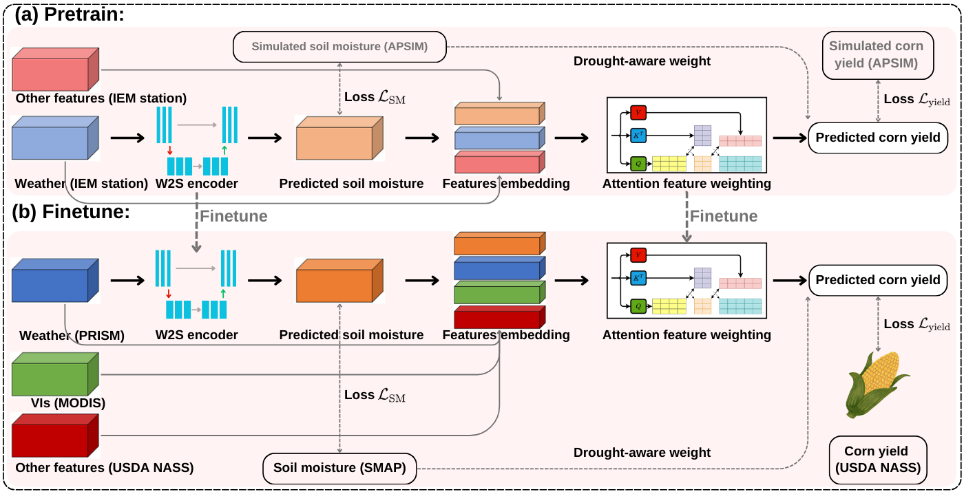
In this paper, we proposed the KGML-SM framework, which integrated PB and ML models for corn yield prediction while incorporating the role of soil moisture in plant growth. The framework consisted of two key components: a Weather-to-Soil (W2S) encoder that modeled the relationship between weather inputs and soil moisture outputs, and an attention module (Vaswani, 2017) that integrated features from multiple sources and dynamically weighted their influence on corn yield across different growth stages and drought conditions. Additionally, we designed a drought-aware yield prediction loss function, informed by the observed relationship between drought and yield reduction, to further enhance model performance under drought conditions. To train this model, we adopted a two-step process. First, we used the APSIM model to generate simulated soil moisture and corn yield data, which were then combined with the input weather data for pretraining. Then, we finetuned the model with soil moisture data from the SMAP product, corn yield data from official statistics, as well as weather data and vegetation indices (VIs) from Google Earth Engine (GEE) (Gorelick et al., 2017), which enabled it to adapt to real-world variability and enhance predictive accuracy. Our research aimed to improve the accuracy and interpretability of corn yield predictions, which ultimately contributed to more resilient agricultural systems in the face of climate variability.
2 Data acquisition
In this study, we developed two datasets for corn yield prediction. The first, a field-level dataset, was generated using APSIM (McCown et al., 1996) and used for pretraining. The second, a county-level dataset, was derived from GEE (Gorelick et al., 2017) and USDA NASS and employed for finetuning. The workflow was divided into three main steps: simulation, pretraining, and finetuning. A summary of all public datasets used in this study is provided in Table 1. In this section, we first introduce the study area (Sec. 2.1); then, we provide details of the APSIM field-level dataset (Sec. 2.2); finally, we describe the construction of the GEE county-level dataset (Sec. 2.3).
| Dataset | Use | Description | References |
| Iowa Environmental Mesonet | a, b | In-situ weather data | (Herzmann et al., 2004) |
| PRISM | c | Gridded weather data | (Daly et al., 2015, 2008) |
| MODIS | c | Vegetation indices | (Justice et al., 1998; Schaaf and Wang, 2015) |
| MODIS MCD18A1.061 | c | Radiation data | (Wang, 2021) |
| USDA-CDL | c | Crop data layer | (USDA-NASS, 2017) |
| SMAP | c | Soil moisture data | (Entekhabi et al., 2010) |
| USDA NASS yield | c | County-level yield | (USDA, 2020) |
2.1 Study area
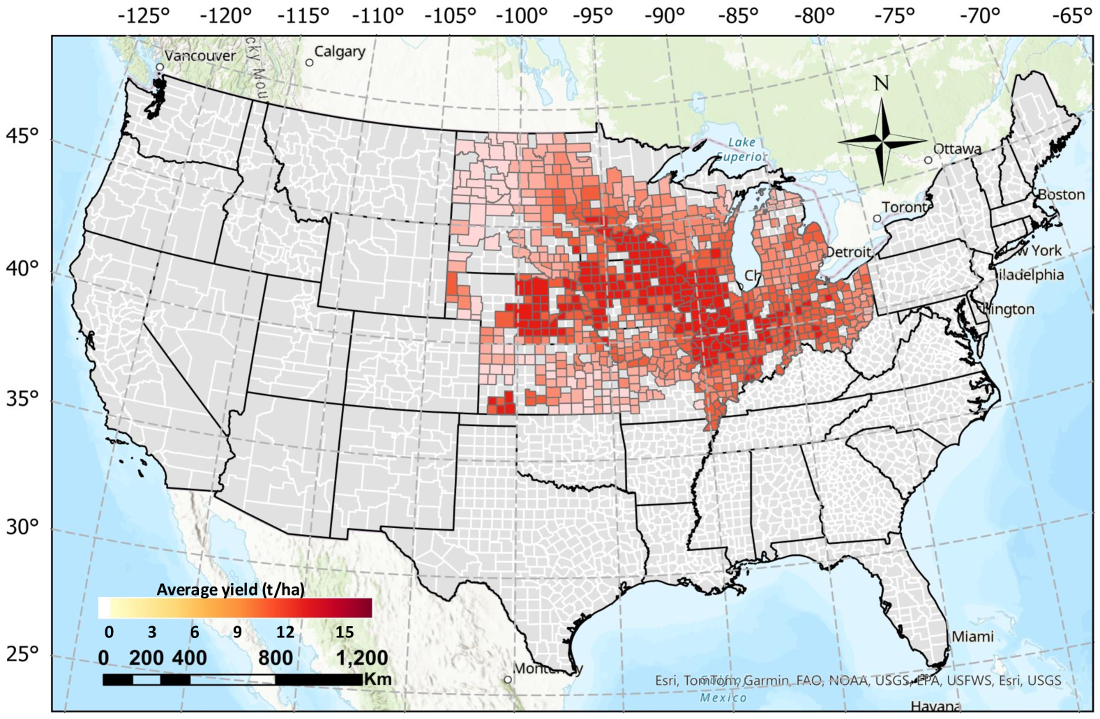
Our research focused on corn yield prediction across the U.S. Corn Belt, selecting twelve states as our study area: North Dakota, South Dakota, Minnesota, Wisconsin, Iowa, Illinois, Indiana, Ohio, Missouri, Kansas, Nebraska, and Michigan. These states are crucial agricultural regions in the U.S., known for their significant contributions to corn production. We generated a five-year average yield map (Fig. 1) for these twelve states and considered them well suited for corn yield prediction research.
2.2 APSIM field-level dataset
In this section, we explain how APSIM was used to generate a field-level simulated dataset for model pretraining. For the simulation of the APSIM field-level dataset, we used data from the Iowa Environmental Mesonet (IEM) (Herzmann et al., 2004), a platform developed by Iowa State University that provides U.S. agricultural and environmental data. We downloaded all available station data from the IEM, which included data from thousands of stations across 12 states from 1980 to 2023 (Table 2).
| State | IA | IL | IN | KS | MI | MN | MO | ND | NE | OH | SD | WI |
| Station number | 113 | 120 | 89 | 150 | 140 | 140 | 130 | 79 | 128 | 100 | 114 | 147 |
2.2.1 Input and output of APSIM
The APSIM model simulates crop yield using four weather data inputs: maximum temperature (Tmax), minimum temperature (Tmin), precipitation (PPT), and radiation (Radn). It also requires certain management parameters, which we describe in detail later (Sec. 3.3.1). Maximum and minimum temperatures influence the rate of plant development and growth stages, impacting processes like photosynthesis and respiration. Precipitation data are essential for modeling soil moisture levels, which directly affect water availability for crops. Radiation is a critical factor in photosynthesis, as it provides the energy needed for plant growth. These weather data are available from the IEM website (Herzmann et al., 2004), which collects and distributes environmental data from various observing networks. The APSIM model takes weather data as input to simulate root zone soil moisture (SM_rootzone), surface soil moisture (SM_surface), and corn yield. SM_rootzone is crucial for corn growth as it directly affects water availability for uptake, influencing plant development and yield. SM_surface plays a key role in seed germination and early growth stages.
2.2.2 Field-level dataset for pretraining
Besides APSIM’s input and output variables, we also extracted two useful features from IEM: prediction year and location (longitude and latitude). Then, we calculated the five-year historical average yield based on the average local simulated corn yield over the past five years. We believed these three features might contribute to improving the accuracy of our corn yield prediction model. After APSIM generated the simulation data, we combined its input weather data, output soil moisture, and corn yield, along with other features to construct the APSIM field-level dataset (Table 3). This dataset was used for pretraining our KGML model, aiming to help the model learn the internal processes of corn growth.
| Category | Variables |
| Weather data | Radn (MJ/m2) (input) |
| Tmax () (input) | |
| Tmin () (input) | |
| PPT (mm) (input) | |
| Soil moisture | SM_surface (simulated) |
| SM_rootzone (simulated) | |
| Corn yield | Corn yield (t/ha) (simulated) |
| Others | Prediction year |
| Location (Latitude and longitude) | |
| Historical average corn yield (t/ha) (simulated) |
2.3 GEE county-level dataset
In this section, we introduce how to construct a county-level dataset for finetuning from GEE. All the variables in the APSIM field-level dataset were also included. To enhance the ML model with RS data, we included VIs from satellite imagery: Green Chlorophyll Index (GCI), Enhanced Vegetation Index (EVI), Normalized Difference Water Index (NDWI), and Normalized Difference Vegetation Index (NDVI).
2.3.1 Vegetation indices
The Moderate Resolution Imaging Spectroradiometer (MODIS) dataset (Justice et al., 1998; Schaaf and Wang, 2015) is a vital source of satellite-derived data with 500 m resolution, providing consistent, high-quality observations of the Earth’s surface. MODIS captures data in multiple spectral bands and offers various products like VIs. These indices are essential for monitoring vegetation health, biomass, water content, and chlorophyll levels across different regions and time scales. They help improve yield prediction by indicating vegetation growth and crop health.
The Green Chlorophyll Index (GCI) is used to estimate the chlorophyll content in plants, which directly relates to plant health and productivity. It is calculated using the near-infrared (NIR) and green spectral bands. GCI is valuable for assessing vegetation health, especially for monitoring crop growth and detecting areas with nutrient deficiencies. High chlorophyll content typically indicates a healthy, productive plant, making GCI an essential tool in agricultural management. GCI is defined as:
| (1) |
where represents the surface reflectance in the Near Infrared band, and represents the surface reflectance in the Green band.
The Enhanced Vegetation Index (EVI) is designed to optimize the vegetation signal by enhancing sensitivity in high biomass areas and reducing atmospheric and canopy background noise. It uses the red, blue, and NIR spectral bands. EVI is particularly useful in regions with dense vegetation, where NDVI might saturate. It provides a more accurate representation of vegetation conditions, especially in areas with high leaf area index, making it ideal for monitoring forests and agricultural lands. EVI is defined as:
| (2) |
where and represent the surface reflectances of the Red band and Blue band, respectively.
The Normalized Difference Water Index (NDWI) measures the moisture content in vegetation and soil by using the NIR and shortwave infrared (SWIR) bands. NDWI is crucial for monitoring water stress in plants, assessing drought conditions, and detecting changes in water bodies. It aids in managing irrigation practices and understanding the impact of water availability on crop yields. NDWI is defined as:
| (3) |
where represents the shortwave infrared band.
The Normalized Difference Vegetation Index (NDVI) is one of the most widely used indices for measuring vegetation greenness and biomass. It is calculated using the NIR and red spectral bands. NDVI is a standard tool for monitoring plant growth, assessing vegetation cover, and detecting changes in biomass over time. It is particularly useful for tracking seasonal variations in vegetation and estimating crop yields. NDVI is defined as:
| (4) |
2.3.2 Weather data
The Parameter-elevation Regressions on Independent Slopes Model (PRISM) dataset (Daly et al., 2015)(Daly et al., 2008) is a high-resolution weather dataset with 4 km resolution that provides detailed information on various climatic variables, including PPT, Tmax, and Tmin. This dataset is widely used in agricultural research, hydrology, and weather studies due to its fine spatial resolution and comprehensive coverage, making it an essential tool for understanding and predicting weather-related impacts on crop yield and other environmental processes.
The MCD18A1 Version 6.1 (Wang, 2021) is a MODIS Terra and Aqua combined Downward Shortwave Radiation gridded Level 3 product that provides us with reliable radiation data (Radn). It is produced daily at 500 m resolution, with estimates of Downward Shortwave Radiation provided every 3 hours. Downward Shortwave Radiation is incident solar radiation over land surfaces in the shortwave spectrum (300-4,000 nanometers) and is an important variable in land-surface models that address a variety of scientific and applied issues.
2.3.3 Soil moisture
The SPL4SMGP.007 SMAP L4 Global 3-hourly 9-km Surface and Root Zone Soil Moisture dataset (Entekhabi et al., 2010) plays a critical role in our research on the relationship between drought and corn yield prediction. By providing detailed measurements of soil moisture at both the surface (0–5 cm) and root zone levels (0–100 cm), SMAP data allows us to assess the availability of water in the soil, a key factor influencing crop growth and resilience during drought conditions.
2.3.4 County-level dataset for finetuning
In addition to the primary weather and vegetation parameters, we also incorporated features such as the prediction year, location (latitude and longitude), and the 5-year historical average yield (USDA, 2020) into our GEE county-level dataset, as in the APSIM field-level dataset. By integrating these features, the model gained a more comprehensive understanding of the environmental and temporal factors affecting corn yield, leading to more reliable predictions. All the variables in GEE county-level dataset are listed in Table 4.
| Category | Variables | Spatial resolution | Source |
| Vegetation index | Green Chlorophyll Index (GCI) | 500m | MODIS |
| Enhanced Vegetation Index (EVI) | |||
| Normalized Difference Water Index (NDWI) | |||
| Normalized Difference Vegetation Index (NDVI) | |||
| Weather data | Radn (W/) | ||
| Tmax () | 4km | PRISM | |
| Tmin () | |||
| PPT (mm) | |||
| Soil moisture | SM_surface | 9km | SMAP |
| SM_rootzone | |||
| Corn yield | USDA NASS corn yield (t/ha) | N/A | USDA NASS |
| Others | Prediction year | ||
| Location (Latitude and longitude) | |||
| Historical average yield (t/ha) |
3 Methodology
The overall pipeline of our KGML-SM is shown in Fig. 2. Our deep learning model consisted of two main components: the W2S encoder, which learned the relationship between weather data and soil moisture, and the attention-based feature-weighting module, which captured how various features influence corn yield. We first pretrained the model using the APSIM field-level dataset, then finetuned it with the GEE county-level dataset.
We begin with a formal Problem formulation of KGML-SM (Sec. 3.1), followed by an introduction to the model components (Sec. 3.2); next, we explain how field-level dataset is generated for pretraining (Sec. 3.3) and county-level dataset for finetuning and testing (Sec. 3.4); finally, we introduce how the KGML model is trained and used for prediction (Sec. 3.5).
3.1 Problem formulation
We formally define the corn yield prediction problem and present its mathematical formulation within a KGML framework. For a unique combination of county and year sample , where , represents all counties across all years in the experiment, we define the input features as follows. The weather features are denoted as , and the other features (prediction year, location, and historical average yield) as , where and represents the entire period from corn planting to harvest. We also have the simulated soil moisture as and denotes the corn yield of each county in that year as supervision. The APSIM field-level dataset, , is used for pretraining. The vertical bar separates the input variables from the target labels.
Additionally, the VIs are represented as . We denote two subsets of the GEE county-level dataset as and respectively, where is used for finetuning and for testing, . Here, we omit the description of the validation set but introduce its partitioning and usage details in the experimental setup (Sec. 4.1).
The objective is to first learn an encoder that maps weather inputs to soil moisture: . Then, the predicted soil moisture is used along with other input features to predict yield through an attention module : . The model’s performance is evaluated by comparing the predicted yields with the actual yields .
3.2 KGML-SM model structure
3.2.1 Weather-to-Soil encoder
W2S encoder is a module designed to model the influence from weather conditions to soil moisture. By capturing the relationship between weather and soil moisture, the W2S encoder enhances the model’s understanding of soil dynamics and the impact of weather variability on soil conditions and corn yield.
The W2S encoder follows a U-Net-based encoder-decoder structure (Ronneberger et al., 2015), consisting of an encoding function , a decoding function , and a final fully connected layer for feature transformation. Given an input time-series weather input , the encoding process can be formulated as:
| (5) |
where denotes the -th convolutional block (LeCun et al., 1995), and represents the max-pooling operation (Nagi et al., 2011) that reduces the temporal dimension. For simplicity we omit the subscript for and .
The decoding process reconstructs high-level features through upsampling and convolutional layers:
| (6) |
where is a transposed convolution (upsampling) operation, represents skip connections concatenating encoder and decoder feature maps, and is the decoder convolutional block.
The predicted soil moisture is obtained via:
| (7) |
3.2.2 Attention module
The attention mechanism (Vaswani, 2017) is a powerful tool in ML that enables models to focus on the most relevant parts of the input data when making predictions. By assigning different levels of importance, or weights, to various input elements, the attention mechanism helps the model prioritize the most crucial information for the task. In KGML-SM, we aim to use the attention mechanism to weight different features, helping us understand each feature’s contribution to yield prediction across different dimensions.
Specifically, suppose that we have input for predicting corn yield. For each feature embedding , we use the attention mechanism to learn the corresponding weight , which is then used to compute the final yield .
First, we compute the query , key , and value vectors from the feature using learned linear transformations:
| (8) |
where , , and are the learned weight matrices for the query, key, and value, respectively.
Next, we calculate the attention scores by taking the dot product of the query and key, scaled by the square root of the key’s dimension :
| (9) |
These attention scores are then passed through a softmax function (Goodfellow et al., 2016) to obtain the weights :
| (10) |
And The softmax function (Goodfellow et al., 2016) is defined as:
| (11) |
Where is the input vector for . is the exponential of the -th element of the input vector .
Finally, we compute the weighted sum of the values to obtain the final yield prediction:
| (12) |
This process allows us to capture the importance of each feature in predicting the yield, dynamically adjusting the weights based on the learned attention scores.
3.3 Generating field-level dataset for pretraining
3.3.1 APSIM management parameters
In addition to weather input data, the APSIM model requires management parameters for calibration. Simulation methods vary depending on the scale of the study. For field-level crop areas, management information is obtained directly from farmers and used as input, while other unknown parameters are adjusted to optimize the model (Shahhosseini et al., 2021). For county-level crop areas, a common practice is to identify representative fields within those counties, average their management parameters, and apply these averages to represent the entire county (Puntel et al., 2016). When the study area is very large, as in our research on simulating all counties in the U.S. Corn Belt, calibrating each county individually became impractical. In this case, the typical approach is to define a range for each parameter based on empirical and statistical data, and then randomly combine these parameters within the specified ranges to simulate yield across all counties (Lobell et al., 2015). Given the vast area of cornfields in our study, it was not feasible to calibrate these parameters for every individual station. Therefore, we established a general range for these parameters to encompass all possible values across different fields. This approach ensured that the model remained applicable to a wide range of conditions while maintaining a reasonable level of accuracy in its predictions.
We selected an appropriate adjustment range for the most important management parameters (Table 5). Sowing density determines the number of plants per unit area, directly affecting competition for resources such as light, water, and nutrients. Based on statistics from the USDA NASS (USDA, 2020), the range for sowing density was set at 6-9 plants/m2. Sowing dates are crucial as they determine the crop’s growth cycle and its interaction with seasonal weather patterns. Typically, growers maximize corn yield by planting in late April or early May (Licht, 2021; Coulter, 2024). In the simulation, sowing started between April 20–25 and ended between May 15–20. Fertilizer application is essential for providing the necessary nutrients to support plant growth. The most commonly used nitrogen fertilizers for corn production in North America are anhydrous ammonia, urea, and urea-ammonium nitrate solutions (Herzmann et al., 2004). The fertilizer amount was set at 200-300 kg/ha of urea nitrogen (N). Initial soil water content is important for establishing the starting conditions for the model’s simulation of soil moisture dynamics throughout the growing season. The initial soil water content was set between 40% and 60%.
| Factor | Value range | Source |
| Start of sowing window | Apr-20 to Apr-25 | (Licht, 2021; Coulter, 2024) |
| End of sowing window | May-15 to May-20 | (Licht, 2021; Coulter, 2024; Lobell et al., 2015) |
| Plant population | 6-9 plants/m2 | (USDA, 2020) |
| Fertilizer amount | 200-300 kg/ha | (Herzmann et al., 2004) |
| Intial soil water | 40%-60% | (Lobell et al., 2015) |
3.3.2 Filtering simulated data based on soil moisture
PB models overlook certain environmental factors and real-world influences, leading to significant discrepancies between some simulated and real-world data. In the simulation process, the simulated intermediate variable is soil moisture, and the final simulation output is corn yield. It is reasonable to assume that with multiple intermediate variables, the final simulation results will have greater errors than the intermediate variables themselves. Additionally, soil moisture is influenced by external factors in a relatively direct manner, unlike yield, which depends on complex plant growth processes. Therefore, soil moisture was used as a benchmark to filter the simulated dataset. We trained a linear regression (LR) model on the GEE county-level dataset to predict soil moisture from weather data and used it to filter the most accurate simulated data in the APSIM field-level dataset. Simulated soil moisture with higher accuracy and its corresponding corn yield were retained to ensure that the model benefited from the most reliable simulations. Notably, we used only simulated data from years before the test year, eliminating the risk of future information leakage.
3.4 Generating county-level dataset for finetuning and testing
3.4.1 Feature Extraction Within Cropland
After downloading various feature data from GEE, we needed to identify the cropland areas. We used the cropland mask from the Cropland Data Layer (CDL) (USDA-NASS, 2017) to extract the feature data corresponding to cropland. The Cropland Data Layer is an annual, raster-based crop-specific land cover dataset produced by the USDA. It has a resolution of 30 meters and offers detailed crop type and location data across the United States. For our corn yield prediction study in twelve U.S. Corn Belt states, we used the CDL to generate a corn field mask in GEE. This mask identifies the specific areas where corn is grown, allowing us to focus our analysis on relevant agricultural fields.
3.4.2 Data preprocessing
Every 16 days, we aggregated all county-level features into a single value to represent agricultural conditions for that period. This method followed the experimental setup from our previous research (Ma et al., 2021b; Wang et al., 2025). We believed that a 16-day interval was sufficient to capture timely changes in weather and environmental conditions.
3.5 Developing the KGML framework
3.5.1 Pretraining with APSIM field-level dataset
The pretraining process began by using a W2S encoder to learn the relationship between input weather features and predicted soil moisture . This process was formulated as . Then, we used the simulated soil moisture to guide the W2S encoder. The loss function was defined as:
| (13) |
where . Next, we concatenated the predicted soil moisture with weather data and other features to form the features embedding . To predict the final corn yield , we used the attention module , which took the concatenated features as input:
| (14) |
The model was trained using the simulated corn yield from the dataset , ensuring that predictions align with PB simulations. The final yield prediction loss function was designed to improve the model’s accuracy while incorporating drought sensitivity and penalizing overestimation. It was formulated as:
| (15) |
where is a drought-aware weighting factor, which was defined as:
| (16) |
where is the average soil moisture over the growing season for sample , and is a small constant to prevent numerical instability. We set in our experiment. Since soil moisture plays a critical role in crop growth and yield formation, the loss function assigned a higher penalty to drier conditions, encouraging the model to be more responsive to soil moisture variations.
Additionally, we incorporated an asymmetric penalty term (Ridnik et al., 2021) controlled by the factor , which amplifies the loss when the predicted yield exceeds the true yield :
| (17) |
This asymmetry discourages overestimation, particularly under drought conditions, where yield predictions tend to be more uncertain. By applying a stronger penalty to overestimated yields, the model is encouraged to be more conservative, reducing the risk of unrealistic predictions. We set in our experiment.
Specifically, when , the predicted error is scaled by a penalty factor , amplifying the loss in these cases. This encourages the model to adopt a conservative approach, reducing the likelihood of overestimating yield, particularly in drought-prone regions where overestimation could lead to inaccurate agricultural planning.
This formulation ensured that the model not only learned accurate yield predictions but also captured the impact of soil moisture variability and drought stress, leading to more reliable and interpretable results.
3.5.2 Finetuning and testing with GEE county-level dataset
We used the GEE county-level dataset for finetuning, which contained real-world input features and corresponding USDA NASS yield records. The loss functions and were optimized on this dataset. Finally, we evaluated the finetuned model on the testing set , where only the input features were available.
4 Experimental Results
4.1 Experimental setup
We conducted experiments on both traditional ML models and DL models. When predicting corn yield for a specific year, we trained the model using all data from preceding years, then split the dataset into 80% for training and 20% for validation, and tested it on the target year. Each experiment was conducted five times with different random seeds, and the final results represented the average across these runs to ensure robustness and reliability.
We implemented the deep learning models using the PyTorch framework (Paszke et al., 2019) and the traditional ML code with sklearn (Pedregosa et al., 2011). The models were run on A100-SXM4-40GB and A100-SXM4-80GB GPUs. For training, we used the ADAM optimizer (Kingma and Ba, 2014) with an initial learning rate of 0.001 and the ReduceLROnPlateau scheduler.
Root mean square error () and the coefficient of determination () were used to evaluate the performance of our model. is a measure of the differences between predicted and actual values in a regression model. It provides an estimate of the standard deviation of the prediction errors. A lower indicates a better fit of the model to the data. The formula for is:
| (18) |
is a statistical measure that indicates the proportion of the variance in the dependent variable that is predictable from the independent variables. An value of 1 indicates perfect prediction, while a value of 0 indicates that the model does not explain any of the variance in the response variable. The formula for is:
| (19) |
where is the number of observations, is the actual value for the -th observation, is the predicted value for the -th observation, and is the mean of the actual values.
4.2 Statistical analysis
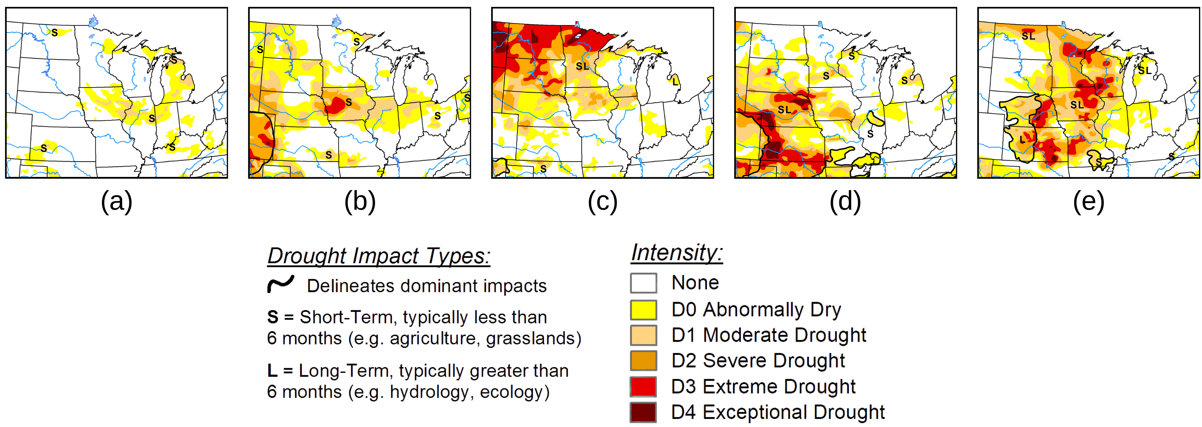
Before conducting the experiments, we analyzed the statistics of drought, soil moisture, and corn yield. We investigated drought conditions in the United States (Drought.gov, 2024) during August from 2019 to 2023 and present the corresponding maps (Fig. 3). While we focused on August, drought conditions throughout the entire corn growing season from May to October were generally similar. In 2019 (Fig. 3(a)), severe drought was primarily observed in Iowa and Michigan. In 2020 (Fig. 3(b)), severe drought affected Iowa, with North Dakota, South Dakota, Nebraska, and Illinois facing moderate drought. 2021 (Fig. 3(c)) saw worsening conditions, with severe drought covering large parts of North Dakota, South Dakota, and Minnesota, while Nebraska and Iowa experienced moderate drought. In 2022 (Fig. 3(d)), severe drought persisted in Nebraska and Kansas, with South Dakota and Iowa experiencing moderate drought. Finally, in 2023 (Fig. 3(e)), severe drought was widespread across Nebraska, Kansas, Minnesota, Iowa, and Wisconsin, while Missouri faced moderate drought conditions.
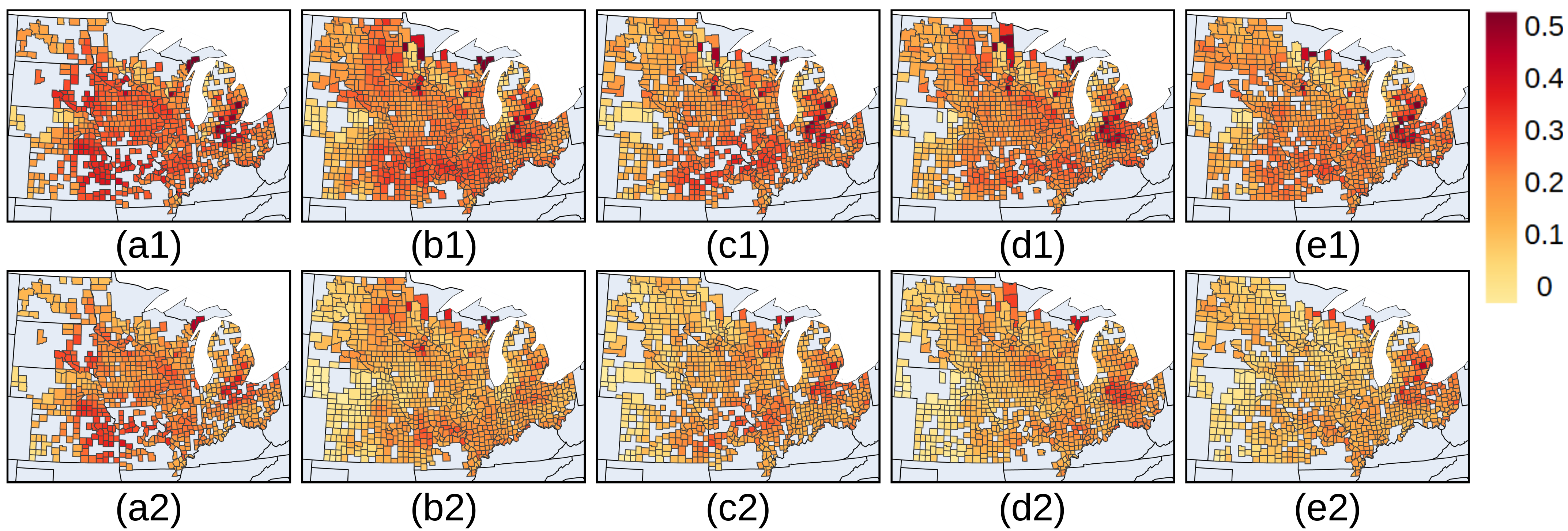
Before studying the impact of soil moisture on corn yield and its prediction, we specified the relationship between soil moisture and drought. Fig. 4 showes the maps of rootzone and surface soil moisture in August from 2019 to 2023. The comparison of the drought maps above with soil moisture data from 2019 to 2023 revealed a strong correlation between drought-affected areas and lower soil moisture levels. We also noticed that rootzone moisture was more abundant than surface moisture and that the two spatial distributions were generally similar.
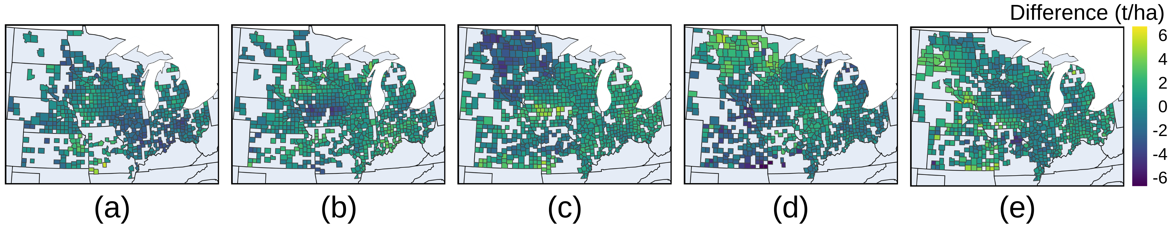
Next, we examined the specific impact of drought on corn yield. We plotted the difference in corn yield for each year from 2019 to 2023 relative to the previous year’s yield (Fig. 5), where negative values indicate a yield reduction. In 2019 (Fig. 5(a)), drought-affected areas included Iowa and Michigan, however, significant yield reductions were observed only in Michigan. In 2020 (Fig. 5(b)), Iowa faced drought along with a derecho storm (Hosseini et al., 2020), leading to noticeable yield losses. In 2021 (Fig. 5(c)), drought impacted North Dakota, South Dakota, Minnesota, Nebraska, and Iowa, yet significant yield reductions occurred only in North Dakota and South Dakota. In 2022 (Fig. 5(d)), drought-affected states included Nebraska, Kansas, South Dakota, and Iowa, but yield declines were primarily observed in North Dakota, Kansas, and South Dakota. In 2023 (Fig. 5(e)), although Nebraska and Kansas continued to experience drought, corn yield did not decrease significantly compared to the previous year, likely due to the already reduced yield in 2022. However, Iowa and Missouri experienced some yield losses due to ongoing drought conditions. Thus, we concluded that drought consistently led to a decline in corn yield. We summarized the drought-affected areas that experienced yield reductions in Table 6. In the experiment, we focused on these states that were affected by drought and experienced yield reductions.
| Drought-affected states | Obviously yield-reduced states | |
| 2019 | IA,MI | MI |
| 2020 | IA,ND,SD,NE,IL | IA |
| 2021 | ND,SD,MN,NE,IA | ND,SD |
| 2022 | NE,KS,SD,IA | NE,KS,SD |
| 2023 | NE,KS,MN,IA,WI,MO | IA,MO |
4.3 KGML-SM performance comparison with traditional ML models
To validate the superiority of our KGML-SM model, we compared it with four traditional machine learning models: LR, multilayer perceptron (MLP), ridge regression (RR), and random forest (RF). LR (Bishop and Nasrabadi, 2006) is a simple statistical method that models the relationship between a dependent variable and one or more independent variables by fitting a linear equation to the data. MLP (Goodfellow et al., 2016) is a neural network with multiple layers, including an input, hidden, and output layer. It captures non-linear relationships and is widely used for classification and regression. RR (Hoerl and Kennard, 1970) is an extension of linear regression that includes an L2 regularization term to prevent overfitting by penalizing large coefficients. RF (Breiman, 2001) is an ensemble learning method that constructs multiple decision trees during training and aggregates their predictions to improve accuracy and robustness.
The results showed that our KGML-SM model consistently outperformed the other ML models across all years (Table 7). Based on the results, RF performed the best among traditional ML models, indicating its strong ability to capture complex relationships in the data. RR performed slightly worse than RF, with slightly higher RMSE values, suggesting that regularization helped improve predictions but was not as effective as ensemble learning. LR ranked next, showing higher RMSE values, likely due to its inability to model non-linear relationships effectively. MLP performed the worst, with the highest RMSE values in most years, indicating that it struggled to generalize well, possibly due to overfitting or insufficient training data.
| KGML-SM | LR | MLP | RR | RF | ||||||
| RMSE | R2 | RMSE | R2 | RMSE | R2 | RMSE | R2 | RMSE | R2 | |
| 2019 | 0.964 | 0.741 | 1.328 | 0.621 | 1.169 | 0.607 | 1.214 | 0.607 | 1.040 | 0.712 |
| 2020 | 0.980 | 0.792 | 1.304 | 0.690 | 1.207 | 0.734 | 1.230 | 0.661 | 1.120 | 0.719 |
| 2021 | 1.104 | 0.836 | 1.167 | 0.790 | 1.247 | 0.761 | 1.129 | 0.808 | 1.236 | 0.794 |
| 2022 | 1.085 | 0.837 | 1.471 | 0.740 | 1.400 | 0.765 | 1.318 | 0.781 | 1.185 | 0.821 |
| 2023 | 1.071 | 0.807 | 1.226 | 0.737 | 1.225 | 0.738 | 1.140 | 0.776 | 1.196 | 0.791 |
4.4 Ablation study of different compoments in KGML-SM model
To further demonstrate the contribution of each module in our KGML-SM model, we conducted a series of ablation studies. We began with a baseline model trained using only the GEE county-level dataset and the attention module (Att) (Wang et al., 2025). Next, we incorporated the simulated dataset to evaluate its impact on model performance (Att+sim). We then introduced the W2S encoder to assess its effectiveness in integrating soil moisture information (Att+sim+W2S). Finally, the impact of the drought-aware loss function was evaluated by comparing the performance of the KGML-SM model with the (Att+sim+W2S) model. We specifically compared the differences among models and their components in Table 8.
| Method | Attention module | Simulated data | W2S encoder | Drought-aware loss |
| Att | ✓ | |||
| Att+sim | ✓ | ✓ | ||
| Att+sim+W2S | ✓ | ✓ | ✓ | |
| KGML-SM | ✓ | ✓ | ✓ | ✓ |
Through an ablation study of all model components (Table 9), we found that the simulated dataset contributed the most to performance improvement. This indicated that our APSIM field-level dataset effectively captured real-world data patterns, playing a crucial role in enabling the model to learn the relationship between corn yield and environmental variables. Additionally, our drought-aware loss function significantly enhanced performance, demonstrating that incorporating prior knowledge of the real-world relationship between drought and corn yield can effectively guide the training and prediction of ML models.
| KGML-SM | Att+sim+W2S | Att+sim | Att | |||||
| RMSE | R2 | RMSE | R2 | RMSE | R2 | RMSE | R2 | |
| 2019 | 0.964 | 0.741 | 0.974 | 0.752 | 1.087 | 0.685 | 1.268 | 0.57 |
| 2020 | 0.98 | 0.792 | 0.981 | 0.783 | 1.003 | 0.77 | 1.011 | 0.77 |
| 2021 | 1.104 | 0.836 | 1.127 | 0.811 | 1.143 | 0.814 | 1.195 | 0.808 |
| 2022 | 1.085 | 0.837 | 1.119 | 0.802 | 1.244 | 0.802 | 1.315 | 0.779 |
| 2023 | 1.071 | 0.807 | 1.101 | 0.805 | 1.114 | 0.781 | 1.201 | 0.766 |
4.5 Spatial Visualization of model performance
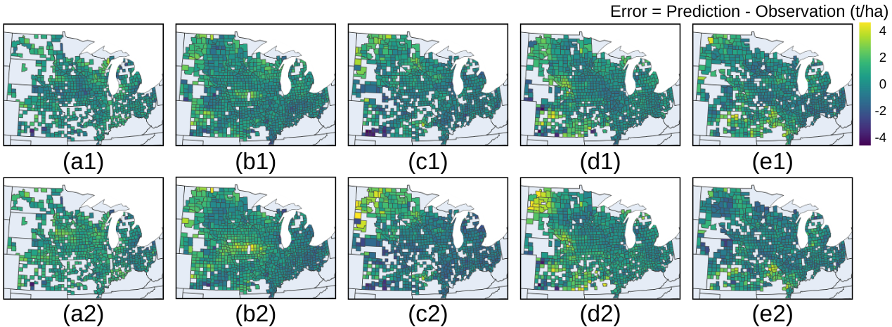
In Fig. 6, we plotted the error maps for the KGML-SM and LR model results from 2019 to 2023. In 2019 (Fig. 6 (a)), the lower part of Michigan shows noticeable overestimation in the attention model, whereas our KGML-SM model performed well. In 2020 (Fig. 6 (b)), although the derecho storm in Iowa also had some impact on our KGML-SM model, we found that the LR model exhibited more severe overestimation. In 2021 (Fig. 6 (c)), overestimation in the upper-left region, particularly in North Dakota and South Dakota, is significantly reduced. In 2022 (Fig. 6 (d)), overestimation decreases notably in South Dakota and Kansas, though the effect in Kansas is less pronounced. In 2023 (Fig. 6 (e)), Missouri showed a clear reduction in overestimation, while the effect in Iowa is less noticeable. Overall, our model shows a notable improvement in addressing the issue of overestimation in drought-affected areas.
4.6 Understanding model bias and prediction-observation alignment
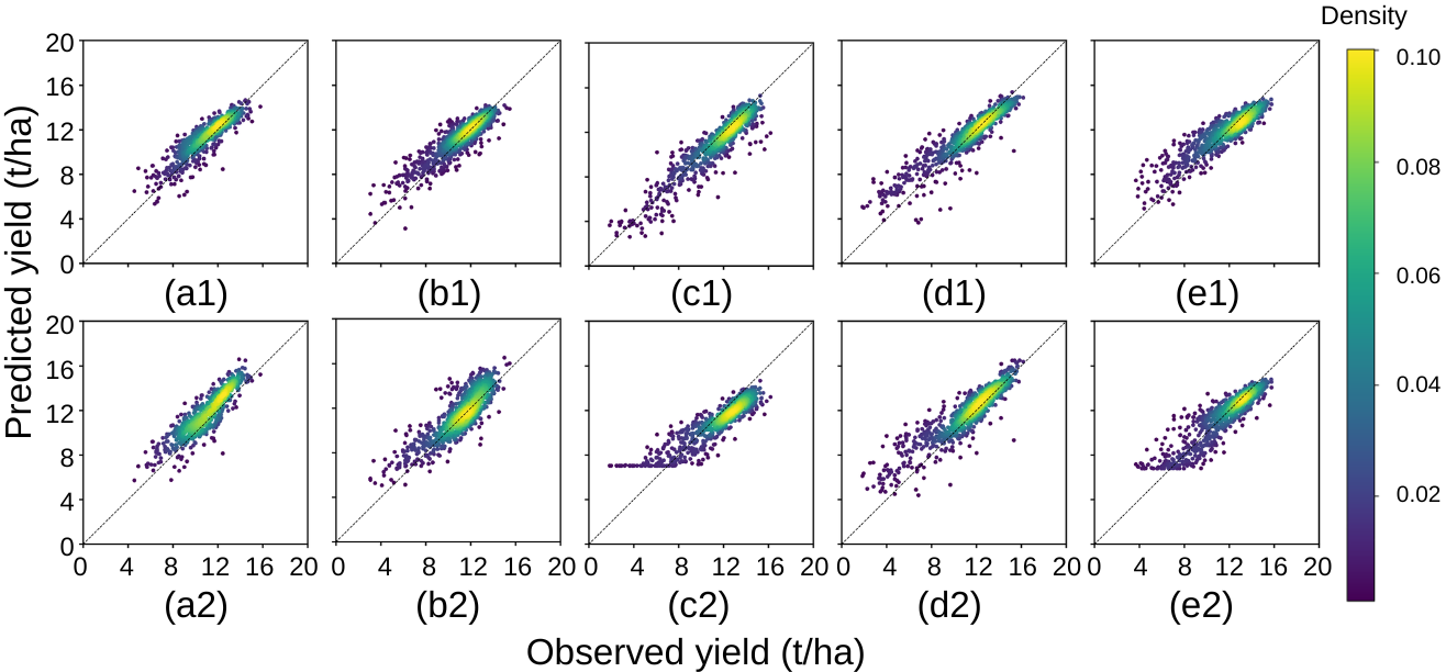
We generated scatter plots for the KGML model and the LR model to analyze their prediction performance (Fig. 7). These plots help visualize the relationship between observed and predicted values, revealing patterns of overestimation, underestimation, and potential prediction biases across different years. In 2019 (Fig. 7 (a)), the KGML-SM model produced a noticeably narrower distribution, indicating a lower spread in prediction errors. In 2020 (Fig. 7 (b)), The predictions of the KGML-SM model were noticeably more concentrated along the diagonal and exhibited symmetry on both sides, whereas the LR model produced more dispersed predictions in high-yield regions. In 2021 (Fig. 7 (c)), the LR model exhibited prediction collapse, where certain observed values correspond to nearly identical predicted values, likely due to overfitting or insufficient variability in learned representations. In 2022 (Fig. 7 (d)), the KGML-SM model maintained a narrower and more concentrated prediction distribution, indicating improved robustness. In 2023 (Fig. 7 (e)), the KGML-SM model continued to avoid prediction collapse, demonstrating more stable performance compared to the attention model. This comparison highlighted the advantage of the KGML-SM model in mitigating prediction collapse and improving overall robustness across different years.
5 Discussion
Specifically, we discussed the role of soil moisture in model prediction from three perspectives:
-
1.
How did soil moisture influence model prediction spatially?
-
2.
How did soil moisture affect model performance throughout the corn growth season?
-
3.
how did soil moisture contribute to model prediction in drought and non-drought regions?
We leveraged the attention mechanism to weight input features, capturing each feature’s contribution to the model, to explore these questions.
5.1 Spatial influence of soil moisture on model prediction
We visualized the attention scores of soil moisture across twelve states in the U.S. Corn Belt from June to August over the years 2019 to 2023 (Fig. 8). The attention scores indicated the relative importance assigned to soil moisture by the model in different regions, with higher scores suggesting a stronger influence on yield prediction. The attention map highlighted how the model’s reliance on soil moisture varied across different growth stages and drought conditions, allowing us to assess whether soil moisture has a greater impact on the model in drought-affected areas.
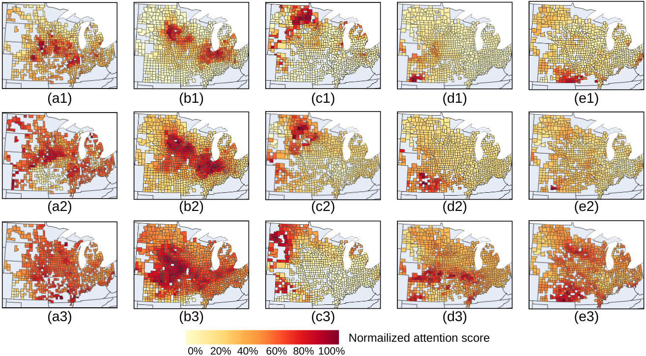
In June, during the early growth period, the attention scores for soil moisture were generally lower across all four years, suggesting that soil moisture is less critical at this stage. This might be due to cooler temperatures and lower evaporation rates, which reduced the immediate need for water. In July, attention scores increased, particularly in drought-affected areas, as soil moisture became more influential during active growth and vegetative stages. By August, attention scores peaked in drought-affected states, aligning with the critical reproductive phase of corn when adequate soil moisture was essential for kernel development.
From 2019 to 2023, the attention distribution of soil moisture in corn yield prediction exhibited noticeable variations, aligning with the drought severity in different years. Note that, for better visualization, we normalized the attention values within each year. Therefore, we only need to focus on the differences across regions within the same year, rather than making cross-year comparisons. In early 2019 (Fig. 8(a1)), the attention was concentrated in Iowa, reflecting the drought-affected states. Subsequently (Fig. 8(a3)), the regions with higher attention values gradually expanded, but Iowa remained the area with the highest attention. In 2020 (Fig. 8(b)), the high-attention regions expanded to include North Dakota, South Dakota, and Nebraska, corresponding to widespread drought in USDA drought map. In 2021 (Fig. 8(c)), the attention intensified over North Dakota, South Dakota, Minnesota, and Nebraska, mirroring severe drought conditions. By 2022 (Fig. 8(d)), high-attention areas were mainly in Nebraska, Kansas, South Dakota, and Iowa. Additionally, over time, there was a trend of drought expanding toward the central region. In 2023 (Fig. 8(e)), the attention peaked across Nebraska, Kansas, Minnesota, Iowa, Wisconsin, and Missouri. Finally, in August, it reached its peak, and soil moisture became more important in most states in the central region.
This above analysis underscored the dynamic role of soil moisture in model prediction, with its importance intensifying during key growth stages and under severe drought conditions. The elevated attention scores in drought-prone regions suggested that soil moisture serves as a crucial predictor for accurately estimating corn yield in water-stressed environments.
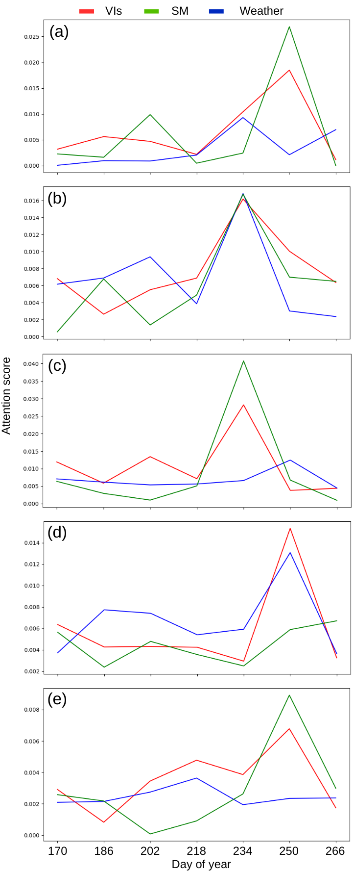
5.2 Temporal role of soil moisture during the corn growth season
To illustrate the impact of soil moisture at different stages of the corn growing season, we visualized the attention of three feature types—VIs, weather, and soil moisture—every 16 days from June to September. We found that the VIs had the highest influence on the model around August, which aligned with findings from previous studies (Johnson, 2014). In this period, VIs shows the strongest correlation with corn yield because this period corresponds to the vegetative and reproductive growth stages, during which crop health and biomass accumulation significantly impact final yield. High VIs in this timeframe indicate optimal chlorophyll content, canopy development, and water availability, which are critical for photosynthesis and grain formation. Additionally, we found that weather data showed a significant increase in attention around July in 2020 and 2022, and the periods with noticeable attention spikes aligned with the trends of VIs. This phenomenon was more pronounced in soil moisture, as soil moisture attention showed a strong correlation with VIs in all years except 2022. In 2022, a slight increase in soil moisture attention could still be observed near the VIs peak. This may be because VIs during these periods are closely related to certain weather data and soil moisture data. For example, NDWI increases with higher PPT because more rainfall enhances soil moisture and plant water content, GCI decreases with excessive Tmax because extreme heat can degrade chlorophyll and reduce plant vitality, etc. This indicated that our attention mechanism effectively captured feature importance over time dimension.
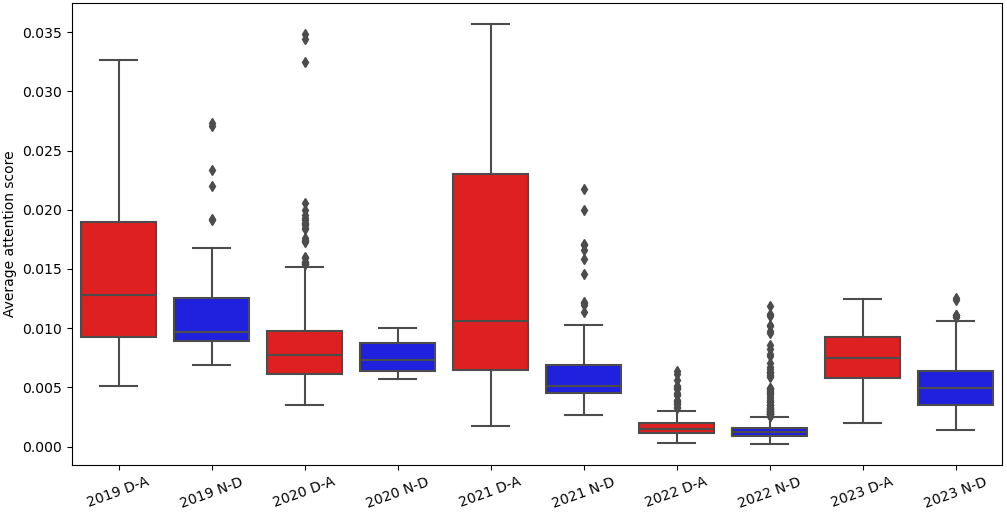
5.3 Statistical impact of soil moisture in drought and non-drought regions
The box plot illustrates the distribution of soil moisture attention across all counties from 2019 to 2023 (Fig. 10). Each point in this box plot represents a county, displaying the comparison of attention between red-marked drought regions and blue-marked non-drought regions from 2019 to 2023. Through this visualization, we aimed to analyze the differences in soil moisture attention between drought-affected and non-drought counties across all years. In 2021, the most severe drought year, both the variance and magnitude of soil moisture attention were the highest. We also observed that attention values were notably high in 2019, which aligns with our experimental results, where our KGML-SM model achieved the most significant improvement over other models. Since our model better captured the impact of soil moisture, it achieved the most significant improvement in years when soil moisture has a greater influence. In contrast, the values for 2020, 2022, and 2023 were more concentrated, with fewer extreme values. Overall, in all years, soil moisture attention in drought-affected regions was consistently higher than in non-drought regions, indicating that soil moisture had a greater impact on the model in these areas.
6 Conclusion
In this study, we proposed the KGML-SM model, which first supplements the limited soil moisture data with simulated data. It then learned the PB relationship between weather and soil moisture. Additionally, based on prior knowledge that drought leads to yield overestimation, we introduced a drought-aware loss function to mitigate this issue in drought-affected areas. We analyzed 12 states in the U.S. Corn Belt to examine the impact of soil moisture on corn yield prediction. Our method consistently outperformed baseline models across multiple test years. We also explore the spatial and temporal impact of soil moisture on the model by visualizing attention, highlighting when and where the model focuses more on soil moisture. In the future, we aim to apply transfer learning to adapt models trained on well-studied regions with simulated data to areas with limited data availability.
References
- Bao et al. (2021) Bao, T., Jia, X., Zwart, J., Sadler, J., Appling, A., Oliver, S., Johnson, T.T., 2021. Partial differential equation driven dynamic graph networks for predicting stream water temperature, in: 2021 IEEE International Conference on Data Mining (ICDM), IEEE. pp. 11–20.
- Bishop and Nasrabadi (2006) Bishop, C.M., Nasrabadi, N.M., 2006. Pattern recognition and machine learning. volume 4. Springer.
- Breiman (2001) Breiman, L., 2001. Random forests. Machine learning 45, 5–32.
- Burroughs et al. (2023) Burroughs, C.H., Montes, C.M., Moller, C.A., Mitchell, N.G., Michael, A.M., Peng, B., Kimm, H., Pederson, T.L., Lipka, A.E., Bernacchi, C.J., et al., 2023. Reductions in leaf area index, pod production, seed size, and harvest index drive yield loss to high temperatures in soybean. Journal of experimental botany 74, 1629–1641.
- Bushong et al. (2016) Bushong, J.T., Mullock, J.L., Miller, E.C., Raun, W.R., Klatt, A.R., Arnall, D.B., 2016. Development of an in-season estimate of yield potential utilizing optical crop sensors and soil moisture data for winter wheat. Precision Agriculture 17, 451–469.
- Chen et al. (2023) Chen, S., Kalanat, N., Xie, Y., Li, S., Zwart, J.A., Sadler, J.M., Appling, A.P., Oliver, S.K., Read, J.S., Jia, X., 2023. Physics-guided machine learning from simulated data with different physical parameters. Knowledge and Information Systems 65, 3223–3250.
- Cooper et al. (2014) Cooper, M., Gho, C., Leafgren, R., Tang, T., Messina, C., 2014. Breeding drought-tolerant maize hybrids for the us corn-belt: discovery to product. Journal of Experimental Botany 65, 6191–6204.
- Coulter (2024) Coulter, J., 2024. Planting date considerations for corn. https://crops.extension.iastate.edu/blog/mark-licht-zachary-clemens/corn-and-soybean-planting-date-considerations.
- Daly et al. (2008) Daly, C., Halbleib, M., Smith, J.I., Gibson, W.P., Doggett, M.K., Taylor, G.H., Curtis, J., Pasteris, P.P., 2008. Physiographically sensitive mapping of climatological temperature and precipitation across the conterminous united states. International Journal of Climatology: a Journal of the Royal Meteorological Society 28, 2031–2064.
- Daly et al. (2015) Daly, C., Smith, J.I., Olson, K.V., 2015. Mapping atmospheric moisture climatologies across the conterminous united states. PloS one 10, e0141140.
- Daw et al. (2022) Daw, A., Karpatne, A., Watkins, W.D., Read, J.S., Kumar, V., 2022. Physics-guided neural networks (pgnn): An application in lake temperature modeling, in: Knowledge Guided Machine Learning. Chapman and Hall/CRC, pp. 353–372.
- Drought.gov (2024) Drought.gov, 2024. U.s. drought monitor. https://www.drought.gov/states/.
- Dugdale et al. (2017) Dugdale, S.J., Hannah, D.M., Malcolm, I.A., 2017. River temperature modelling: A review of process-based approaches and future directions. Earth-Science Reviews 175, 97–113.
- Entekhabi et al. (2010) Entekhabi, D., Njoku, E.G., O’neill, P.E., Kellogg, K.H., Crow, W.T., Edelstein, W.N., Entin, J.K., Goodman, S.D., Jackson, T.J., Johnson, J., et al., 2010. The soil moisture active passive (smap) mission. Proceedings of the IEEE 98, 704–716.
- Goodfellow et al. (2016) Goodfellow, I., Bengio, Y., Courville, A., 2016. Deep learning. MIT press.
- Gorelick et al. (2017) Gorelick, N., Hancher, M., Dixon, M., Ilyushchenko, S., Thau, D., Moore, R., 2017. Google earth engine: Planetary-scale geospatial analysis for everyone. Remote Sensing of Environment URL: https://doi.org/10.1016/j.rse.2017.06.031, doi:10.1016/j.rse.2017.06.031.
- Graham et al. (2007) Graham, R.L., Nelson, R., Sheehan, J., Perlack, R.D., Wright, L.L., 2007. Current and potential us corn stover supplies. Agronomy Journal 99, 1–11.
- He et al. (2023) He, E., Xie, Y., Liu, L., Chen, W., Jin, Z., Jia, X., 2023. Physics guided neural networks for time-aware fairness: an application in crop yield prediction, in: Proceedings of the AAAI Conference on Artificial Intelligence, pp. 14223–14231.
- He et al. (2016) He, K., Zhang, X., Ren, S., Sun, J., 2016. Deep residual learning for image recognition, in: Proceedings of the IEEE conference on computer vision and pattern recognition, pp. 770–778.
- Herzmann et al. (2004) Herzmann, D., Arritt, R., Todey, D., 2004. Iowa environmental mesonet. Available at mesonet. agron. iastate. edu/request/coop/fe. phtml (verified 27 Sept. 2005). Iowa State Univ., Dep. of Agron., Ames, IA .
- Hoerl and Kennard (1970) Hoerl, A.E., Kennard, R.W., 1970. Ridge regression: Biased estimation for nonorthogonal problems. Technometrics 12, 55–67.
- Hosseini et al. (2020) Hosseini, M., Kerner, H.R., Sahajpal, R., Puricelli, E., Lu, Y.H., Lawal, A.F., Humber, M.L., Mitkish, M., Meyer, S., Becker-Reshef, I., 2020. Evaluating the impact of the 2020 iowa derecho on corn and soybean fields using synthetic aperture radar. Remote Sensing 12, 3878.
- Ines et al. (2013) Ines, A.V., Das, N.N., Hansen, J.W., Njoku, E.G., 2013. Assimilation of remotely sensed soil moisture and vegetation with a crop simulation model for maize yield prediction. Remote Sensing of Environment 138, 149–164.
- Johnson (2014) Johnson, D.M., 2014. An assessment of pre-and within-season remotely sensed variables for forecasting corn and soybean yields in the united states. Remote Sensing of Environment 141, 116–128.
- Jones et al. (2003) Jones, J.W., Hoogenboom, G., Porter, C.H., Boote, K.J., Batchelor, W.D., Hunt, L., Wilkens, P.W., Singh, U., Gijsman, A.J., Ritchie, J.T., 2003. The dssat cropping system model. European journal of agronomy 18, 235–265.
- Justice et al. (1998) Justice, C.O., Vermote, E., Townshend, J.R., Defries, R., Roy, D.P., Hall, D.K., Salomonson, V.V., Privette, J.L., Riggs, G., Strahler, A., et al., 1998. The moderate resolution imaging spectroradiometer (modis): Land remote sensing for global change research. IEEE transactions on geoscience and remote sensing 36, 1228–1249.
- Karpatne et al. (2022) Karpatne, A., Kannan, R., Kumar, V., 2022. Knowledge guided machine learning: Accelerating discovery using scientific knowledge and data. CRC Press.
- Kimball et al. (2023) Kimball, B.A., Thorp, K.R., Boote, K.J., Stockle, C., Suyker, A.E., Evett, S.R., Brauer, D.K., Coyle, G.G., Copeland, K.S., Marek, G.W., et al., 2023. Simulation of evapotranspiration and yield of maize: An inter-comparison among 41 maize models. Agricultural and Forest Meteorology 333, 109396.
- Kingma and Ba (2014) Kingma, D.P., Ba, J., 2014. Adam: A method for stochastic optimization. arXiv preprint arXiv:1412.6980 .
- Kucharik and Ramankutty (2005) Kucharik, C.J., Ramankutty, N., 2005. Trends and variability in us corn yields over the twentieth century. Earth Interactions 9, 1–29.
- LeCun et al. (1995) LeCun, Y., Bengio, Y., et al., 1995. Convolutional networks for images, speech, and time series. The handbook of brain theory and neural networks 3361, 1995.
- Licheng et al. (2022) Licheng, L., Zhou, W., Jin, Z., Tang, J., Jia, X., Jiang, C., Guan, K., Peng, B., Xu, S., Yang, Y., et al., 2022. Estimating the autotrophic and heterotrophic respiration in the us crop fields using knowledge guided machine learning. Authorea Preprints .
- Licht (2021) Licht, M., 2021. Corn and soybean planting date considerations. https://crops.extension.iastate.edu/blog/mark-licht-zachary-clemens/corn-and-soybean-planting-date-considerations.
- Lobell et al. (2015) Lobell, D.B., Thau, D., Seifert, C., Engle, E., Little, B., 2015. A scalable satellite-based crop yield mapper. Remote Sensing of Environment 164, 324–333.
- Luo et al. (2023) Luo, Y., Liu, Q., Chen, Y., Hu, W., Tian, T., Zhu, J., 2023. Physics-guided discovery of highly nonlinear parametric partial differential equations, in: Proceedings of the 29th ACM SIGKDD Conference on Knowledge Discovery and Data Mining, pp. 1595–1607.
- Ma et al. (2021a) Ma, Y., Zhang, Z., Kang, Y., Özdoğan, M., 2021a. Corn yield prediction and uncertainty analysis based on remotely sensed variables using a bayesian neural network approach. Remote Sensing of Environment 259, 112408.
- Ma et al. (2021b) Ma, Y., Zhang, Z., Kang, Y., Özdoğan, M., 2021b. Corn yield prediction and uncertainty analysis based on remotely sensed variables using a bayesian neural network approach. Remote Sensing of Environment 259, 112408.
- McCown et al. (1996) McCown, R.L., Hammer, G.L., Hargreaves, J.N.G., Holzworth, D.P., Freebairn, D.M., 1996. Apsim: a novel software system for model development, model testing and simulation in agricultural systems research. Agricultural systems 50, 255–271.
- Mladenova et al. (2017) Mladenova, I.E., Bolten, J.D., Crow, W.T., Anderson, M.C., Hain, C.R., Johnson, D.M., Mueller, R., 2017. Intercomparison of soil moisture, evaporative stress, and vegetation indices for estimating corn and soybean yields over the us. IEEE Journal of Selected Topics in Applied Earth Observations and Remote Sensing 10, 1328–1343.
- Nagi et al. (2011) Nagi, J., Ducatelle, F., Di Caro, G.A., Cireşan, D., Meier, U., Giusti, A., Nagi, F., Schmidhuber, J., Gambardella, L.M., 2011. Max-pooling convolutional neural networks for vision-based hand gesture recognition, in: 2011 IEEE international conference on signal and image processing applications (ICSIPA), IEEE. pp. 342–347.
- Paszke et al. (2019) Paszke, A., Gross, S., Massa, F., Lerer, A., Bradbury, J., Chanan, G., Killeen, T., Lin, Z., Gimelshein, N., Antiga, L., et al., 2019. Pytorch: An imperative style, high-performance deep learning library. Advances in neural information processing systems 32.
- Pedregosa et al. (2011) Pedregosa, F., Varoquaux, G., Gramfort, A., Michel, V., Thirion, B., Grisel, O., Blondel, M., Prettenhofer, P., Weiss, R., Dubourg, V., Vanderplas, J., Passos, A., Cournapeau, D., Brucher, M., Perrot, M., Duchesnay, E., 2011. Scikit-learn: Machine learning in Python. Journal of Machine Learning Research 12, 2825–2830.
- Pignotti et al. (2023) Pignotti, G., Crawford, M., Han, E., Williams, M.R., Chaubey, I., 2023. Smap soil moisture data assimilation impacts on water quality and crop yield predictions in watershed modeling. Journal of Hydrology 617, 129122.
- Puntel et al. (2016) Puntel, L.A., Sawyer, J.E., Barker, D.W., Dietzel, R., Poffenbarger, H., Castellano, M.J., Moore, K.J., Thorburn, P., Archontoulis, S.V., 2016. Modeling long-term corn yield response to nitrogen rate and crop rotation. Frontiers in plant science 7, 1630.
- Ridnik et al. (2021) Ridnik, T., Ben-Baruch, E., Zamir, N., Noy, A., Friedman, I., Protter, M., Zelnik-Manor, L., 2021. Asymmetric loss for multi-label classification, in: Proceedings of the IEEE/CVF international conference on computer vision, pp. 82–91.
- Ronneberger et al. (2015) Ronneberger, O., Fischer, P., Brox, T., 2015. U-net: Convolutional networks for biomedical image segmentation, in: Medical image computing and computer-assisted intervention–MICCAI 2015: 18th international conference, Munich, Germany, October 5-9, 2015, proceedings, part III 18, Springer. pp. 234–241.
- Schaaf and Wang (2015) Schaaf, C., Wang, Z., 2015. Mcd43a4 modis/terra+ aqua brdf/albedo nadir brdf adjusted ref daily l3 global-500m v006. nasa eosdis land processes daac. USGS Earth Resources Observation and Science (EROS) Center, Sioux Falls, South Dakota (https://lpdaac. usgs. gov) .
- Shahhosseini et al. (2021) Shahhosseini, M., Hu, G., Huber, I., Archontoulis, S.V., 2021. Coupling machine learning and crop modeling improves crop yield prediction in the us corn belt. Scientific reports 11, 1606.
- Thompson (1969) Thompson, L.M., 1969. Weather and technology in the production of corn in the us corn belt 1. Agronomy Journal 61, 453–456.
- Unganai and Kogan (1998) Unganai, L.S., Kogan, F.N., 1998. Drought monitoring and corn yield estimation in southern africa from avhrr data. Remote sensing of environment 63, 219–232.
- USDA (2020) USDA, 2020. United states department of agriculture national agricultural statistics service .
- USDA-NASS (2017) USDA-NASS, C., 2017. Usda national agricultural statistics service cropland data layer .
- Van Diepen et al. (1989) Van Diepen, C.v., Wolf, J.v., Van Keulen, H., Rappoldt, C., 1989. Wofost: a simulation model of crop production. Soil use and management 5, 16–24.
- Vaswani (2017) Vaswani, A., 2017. Attention is all you need. arXiv preprint arXiv:1706.03762 .
- Vergopolan et al. (2021) Vergopolan, N., Xiong, S., Estes, L., Wanders, N., Chaney, N.W., Wood, E.F., Konar, M., Caylor, K., Beck, H.E., Gatti, N., et al., 2021. Field-scale soil moisture bridges the spatial-scale gap between drought monitoring and agricultural yields. Hydrology and Earth System Sciences 25, 1827–1847.
- Wang et al. (2018) Wang, A.X., Tran, C., Desai, N., Lobell, D., Ermon, S., 2018. Deep transfer learning for crop yield prediction with remote sensing data, in: Proceedings of the 1st ACM SIGCAS Conference on Computing and Sustainable Societies, pp. 1–5.
- Wang (2021) Wang, D., 2021. Modis/terra+aqua surface radiation daily/3-hour l3 global 1km sin grid v061 [data set]. NASA EOSDIS Land Processes Distributed Active Archive Center. (https://lpdaac. usgs. gov) .
- Wang et al. (2025) Wang, X., Ma, Y., Xu, Y., Huang, Q., Yang, Z., Zhang, Z., 2025. Learning county from pixels: Corn yield prediction with attention-weighted multiple instance learning. International Journal of Remote Sensing , 1–31.
- Weiss et al. (2007) Weiss, M., Baret, F., Garrigues, S., Lacaze, R., 2007. Lai and fapar cyclopes global products derived from vegetation. part 2: validation and comparison with modis collection 4 products. Remote Sensing of Environment 110, 317–331. URL: https://www.sciencedirect.com/science/article/pii/S0034425707000910, doi:https://doi.org/10.1016/j.rse.2007.03.001.
- Weiss et al. (2002) Weiss, M., Baret, F., Leroy, M., Hautecœur, O., Bacour, C., Prevol, L., Bruguier, N., 2002. Validation of neural net techniques to estimate canopy biophysical variables from remote sensing data. Agronomie-Sciences des Productions Vegetales et de l’Environnement 22, 547–554.
- Weiss et al. (2004) Weiss, M., Baret, F., Smith, G., Jonckheere, I., Coppin, P., 2004. Review of methods for in situ leaf area index (lai) determination: Part ii. estimation of lai, errors and sampling. Agricultural and Forest Meteorology 121, 37–53. URL: https://www.sciencedirect.com/science/article/pii/S0168192303001631, doi:https://doi.org/10.1016/j.agrformet.2003.08.001.
- Weiss et al. (2020) Weiss, M., Jacob, F., Duveiller, G., 2020. Remote sensing for agricultural applications: A meta-review. Remote sensing of environment 236, 111402.
- Williams and Izaurralde (2010) Williams, J.R., Izaurralde, R.C., 2010. The apex model, in: Watershed models. CRC Press, pp. 461–506.
- Yang et al. (2023) Yang, Q., Liu, L., Zhou, J., Ghosh, R., Peng, B., Guan, K., Tang, J., Zhou, W., Kumar, V., Jin, Z., 2023. A flexible and efficient knowledge-guided machine learning data assimilation (kgml-da) framework for agroecosystem prediction in the us midwest. Remote Sensing of Environment 299, 113880.
- Yang et al. (2024) Yang, Q., Liu, L., Zhou, J., Rogers, M., Jin, Z., 2024. Predicting the growth trajectory and yield of greenhouse strawberries based on knowledge-guided computer vision. Computers and Electronics in Agriculture 220, 108911.
- You et al. (2017) You, J., Li, X., Low, M., Lobell, D., Ermon, S., 2017. Deep gaussian process for crop yield prediction based on remote sensing data, in: Proceedings of the AAAI conference on artificial intelligence.
- Zhen et al. (2023) Zhen, X., Huo, W., Tian, D., Zhang, Q., Sanz-Saez, A., Chen, C.Y., Batchelor, W.D., 2023. County level calibration strategy to evaluate peanut irrigation water use under different climate change scenarios. European Journal of Agronomy 143, 126693.
- Zhen et al. (2022) Zhen, X., Zhang, Q., Sanz-Saez, A., Chen, C.Y., Dang, P.M., Batchelor, W.D., 2022. Simulating drought tolerance of peanut varieties by maintaining photosynthesis under water deficit. Field Crops Research 287, 108650.