Many exact area-law scar eigenstates in the nonintegrable PXP and related models

Abstract

In this work, we present new, highly non-trivial area-law exact zero-energy eigenstates of the one-dimensional (1D) PXP and related models. We formulate sufficient conditions for a matrix product state to represent an exact zero-energy eigenstate of a given 1D kinetically constrained model and use them to prove our new states. We also demonstrate that all previously known exact eigenstates of PXP-type models satisfy these conditions, and, in fact, can be directly deduced from them. We discuss and demonstrate a remarkably effective general numerical technique for discovering finite-bond-dimension eigenstates residing in degenerate subspaces of a broad class of Hamiltonians. Our results highlight a previously unrecognized structure characteristic of the exponentially large nullspaces in kinetically constrained models, suggesting the possibly of extensively many increasingly complex area-law zero-energy eigenstates in the thermodynamic limit. The important implications of these emergent exact eigenstates for the general thermalization phenomenology are exemplified by one of the states introduced in this work, which we propose is a member of the primary $\mathbb{Z}_{2}$ quantum many-body scar tower responsible for long-lived revivals in the Rydberg atom chain experiment.

I Introduction

Questions of integrability and thermalization of models with local kinetic constraints, which restrict the allowed state space, have been at the forefront of research for several decades. More recently, models characterized by the Rydberg blockade constraint, naturally arising in experiments with trapped neutral cold atoms, have attracted significant attention. This surge of interest followed the observation of unexpected many-body revivals of the Néel-type $\ket{\mathbb{Z}_{2}}$ state in the quench experiment [Bernien_2017], and the subsequent attribution of that dynamics to the eigenstate thermalization hypothesis (ETH) violations in the one-dimensional (1D) PXP Hamiltonian, which encapsulates the essential physics of the Rydberg atomic system [Turner_2018weak, Turner_2018quantum]. Specifically, a quantum many-body scar (QMBS) tower of approximately equally spaced states featuring sub-extensive scaling of entanglement entropy and high overlaps with $\ket{\mathbb{Z}_{2}}$ (in comparison to the nearby states) was discovered in the spectrum of the PXP Hamiltonian and shown to play a key role in the observable non-ergodic phenomenology. A very recent discovery of similar approximate scar towers featuring analogous oscillatory dynamical signatures in a broader family of PXP-type models with longer-range constraints [kerschbaumer2024quantummanybodyscarspxp] further highlighted the ubiquity of scarring in kinetically constrained models.

Although the absence of local conserved quantities in the PXP model was demonstrated recently, suggesting its nonintegrability [Park_2024], several exact eigenstates were nonetheless identified within the model’s exponentially large nullspace [lin2019exact, Ivanov_2025]. Over the years, numerous efforts have been made to uncover additional exact scars in PXP-type models, employing a wide range of techniques. These include identifying states with anomalously low Schmidt ranks through ED [Moudgalya_2018, lin2019exact], entanglement minimization within the nullspace [Karle_2021], machine learning [Szo_dra_2022, feng2024uncoveringquantummanybodyscars], correlation matrix analysis [yao2024quantummanybodyscarslens], analytic continuation of the partition function and Fisher zeros [meng2025detectingmanybodyscarsfisher], and DMRG methods [Zhang_2023, yuan2023exactquantummanybodyscars]. However, the absence of new exact results beyond the states reported in Refs. [lin2019exact] and [Surace_2021] raises a critical question: Do other exact scars exist, and if so, how can they be detected?

We address this question by seeking to uncover an underlying structure that allows the existence of exact scars within the (symmetry-protected) exponentially degenerate nullspaces [Schecter_2018] of the PXP-type as well as more general kinetically constrained models. Our pursuit of new exact analytical results stems from the aspiration to gain fresh insights into existing examples of ergodicity-breaking phenomena in these models (in particular, in the thermodynamic limit), and to uncover previously hidden features. We also aim to enhance our understanding of the limits of exact solvability and integrability within this important family of Hamiltonians. Our new numerical method for finding exact scars in such highly degenerate nullspaces, while remarkably successful in uncovering the new states presented in this work, also highlights the inherent hardness of this endeavor, which perhaps carries deeper implications by itself. As a by-product, building on top of one of our new scars in the PXP chain, we find the most accurate theoretical description to date of the primary $\mathbb{Z}_{2}$ scars with non-zero energies framing the nullspace. This allows us to also provide a new perspective on the long-lived oscillating revivals in quenches from the $\mathbb{Z}_{2}$ charge density wave (CDW) states.

This paper is organized as follows. In Sec. II we review the family of 1D models with Rydberg blockade constrains, which includes the PXP and PPXPP models that are of main focus in this work. Then in Sec. III we define several distinct types of translationally-invariant (TI) matrix product state (MPS) representations, which, in the following Sec. IV, are used to express and characterize all presently known exact TI eigenstates of the two models. Note that our new scar eigenstates will be initially introduced and discussed in some detail without proofs. We will establish the proofs in Sec V in the form of conditions sufficient for an MPS to represent an exact zero energy eigenstate of a Hamiltonian with a local kinetic constraint. There, we will show that all the states listed in Sec. IV (both new and previously known) satisfy a particular set of nonlinear matrix equations, which can be deduced from the type of the state’s MPS representation and the properties of the Hamiltonian. In Sec. LABEL:sec:extra, to further highlight the generality of the formalism developed in Sec. V, we will provide several additional examples involving models and situations not considered earlier. In Sec. LABEL:sec:detection, we present a systematic numerical technique for detecting area-law-entangled states in exponentially degenerate subspaces and provide its demonstration using the PXP Hamiltonian as an example. Finally, in Sec. LABEL:sec:dynamics, we provide a new perspective on the extensively studied non-ergodic dynamics associated with the primary $\mathbb{Z}_{2}$ scars in the PXP model by demonstrating its connection to some of our newly introduced states.

II Models

The PXP model, which is an idealized description of Rydberg atomic systems in the nearest-neighbor blockade regime, is defined for a spin-1/2 chain of length $L$ by the following Hamiltonian:

$$H_{\text{PXP}}=\sum_{j=2}^{L-1}P_{j-1}X_{j}P_{j+1}+H_{\text{left}}+H_{\text{right}},$$ (1)

where $P_{i}=\outerproduct{0}{0}_{i}$, $X_{i}=\outerproduct{1}{0}_{i}+\outerproduct{0}{1}_{i}$; for PBC $H_{\text{left}}=P_{L}X_{1}P_{2}$ and $H_{\text{right}}=P_{L-1}X_{L}P_{1}$, whereas for open boundary conditions (OBC) $H_{\text{left}}=X_{1}P_{2}$ and $H_{\text{right}}=P_{L-1}X_{L}$. A natural generalization of the PXP Hamiltonian (assuming PBC) with the blockade radius parametrized by an integer $\alpha$ is the following:

$$H^{\alpha}=\sum_{j=1}^{L}P_{j-\alpha}\dots P_{j-1}X_{j}P_{j+1}\dots P_{j+\alpha}.$$ (2)

Clearly, $H_{\text{PXP}}=H^{1}$, whereas $H^{2}$ corresponds to the so-called PPXPP model [Surace_2021, Karle_2021]. Any $H^{\alpha}$ has a dynamically decoupled subspace

$$\mathcal{H}^{\alpha}=\operatorname{span}\big{\{}\ket{s_{1}s_{2}\cdots s_{L}}:\begin{aligned} &s_{i}s_{i+k}\neq 11,\\ &\text{for any }i,k=1..\alpha\big{\}},\end{aligned}$$ (3)

which, due its experimental relevance, will be our focus.

Hamiltonians $H^{\alpha}$ possess three conventional symmetries: translational symmetry for the case of PBC, which we will denote by $T_{x}$; inversion symmetry $\mathcal{I}$ about any axis cutting the chain into two equal parts; and spectral reflection symmetry defined by the operator $\mathcal{C}=\prod_{j}Z_{j}$, where $Z=\outerproduct{0}{0}-\outerproduct{1}{1}$. Since $\left\{\mathcal{C},H^{\alpha}\right\}=0$, the spectrum of $H^{\alpha}$ is symmetric about $E=0$. Moreover, all Hamiltonians $H^{\alpha}$ possess exponentially degenerate nullspaces as a result of the interplay between the $\mathcal{I}$ and $\mathcal{C}$ symmetries [Turner_2018quantum, Buijsman_2022].

Some parts of our discussion will be more natural in the blocked basis where, following the notation of Ref. [lin2019exact], composite two-spin states $\ket{00}$, $\ket{01}$, and $\ket{10}$ are denoted by $\ket{O}$, $\ket{R}$, and $\ket{L}$. For example, in this blocked basis the PXP Hamiltonian for a PBC chain of size $L=2L_{b}$ can be written as the following sum of one-body and two-body terms:

$$H_{\mathrm{PXP}}=H_{1}+H_{2},$$ (4)

where (assuming the block-site index $j$ refers to two-atom blocks)

$$H_{1} =\sum_{j=1}^{L_{b}}\left\{\left(\ket{O}\left[\bra{L}+\bra{R}\right]\right)_{j}+\mathrm{h.c.}\right\},$$ (5a)

$$H_{2} =-\sum_{j=1}^{L_{b}}\left\{\left(\ket{RL}\left[\bra{OL}+\bra{RO}\right]\right)_{j,j+1}+\mathrm{h.c.}\right\}.$$ (5b)

With summation in Eq. (5b) truncated at $L_{b}-1$, this representation is also valid for OBC.

The blocked basis is natural for representing the exact translational-symmetry-breaking eigenstates PBC states $\ket{\Phi_{1}}$ and $\ket{\Phi_{2}}$ from Ref. [lin2019exact], as well as some of the new eigenstates of both the PXP and PPXPP models to be introduced later. Such states are intimately connected to the $H_{1}$ term in Eq. (5a), which, in contrast to the $H_{\text{PXP}}$ and the $H_{2}$ term, is an integrable Hamiltonian. We will elaborate on the details of this connection later. In what follows, we will often denote various TI Hamiltonians with terms acting on single sites in a particular basis by $H_{1}$.

III Types of MPS representations

III.1 TI MPS

It is known that any translationally-invariant in a particular local basis $\{\ket{s}\}$ state $\ket{\psi}$ can be expressed as a TI MPS with site-independent matrices $M^{s}$ as follows [perez2007matrix]:

$$\ket{\psi}=\sum_{\{s_{i}\}}\Tr{M^{s_{1}}M^{s_{2}}\cdots M^{s_{L_{b}}}}\ket{s_{1}s_{2}\dots s_{L_{b}}}.$$ (6)

When defining states via Eq. (6) we will use either the single-site basis $\{\ket{0},\ket{1}\}$, or, as in Ref. [lin2019exact], the blocked basis $\{\ket{O},\ket{L},\ket{R}\}\equiv\{\ket{00},\ket{10},\ket{01}\}$ representing blocks consisting of adjacent spin-1/2 sites subject to the Rydberg blockade .

III.2 Blocked-antipodal (BA) TI MPS

Volume-entangled states with well-defined antipodal structure like the ones discussed in Refs. [Ivanov_2025, Chiba_2024, yoneta2024thermalpurestatessystems] can be expressed in what we will call the BA basis as follows:

$$\ket{\psi}=\sum_{\{s_{i},s_{\overline{i}}\}} \Tr{M^{s_{1}s_{\overline{1}}}M^{s_{2}s_{\overline{2}}}\cdots M^{s_{L_{b}}s_{\overline{L_{b}}}}}$$ (7)

$$\times\ket{s_{1}s_{2}\dots s_{L_{b}}}\otimes\ket{s_{\overline{1}}s_{\overline{2}}\dots s_{\overline{L_{b}}}},$$

where $s_{i},s_{\overline{i}}\in\{0,1\}$ and the sites in the second line are adjacent to each other on a chain with PBCs (see Fig. 1 in Ref. [Ivanov_2025]). Note that the BA representation generates TI states only when $M^{s_{i}s_{\overline{i}}}=M^{s_{\overline{i}}s_{i}}$.

III.3 Twisted translationally-invariant (TTI) MPS

We stated earlier that any TI state has a TI MPS representation. It is, however, not always possible to write such states, even those with finite Schmidt index in the thermodynamic limit, using system-size-independent tensors. This striking deficiency of the standard TI MPS representation is famously exemplified by the so-called $W$-state given by

$$\ket{W}=\left(\frac{1}{\sqrt{L}}\sum_{i=1}^{L}X_{i}\right)\ket{00\dots 0}.$$ (8)

It is known that the TI MPS representation of the $W$-state, whose Schmidt index is 2, requires system-size-dependent tensors with bond dimension $\chi\succeq\mathcal{O}(L^{1/3})$ [perez2007matrix]; there is also more recent evidence suggesting that in the best case $\chi=\lfloor L/2\rfloor+1$ [klimov2023translationinvariantmatrixproductstates]. Leaving the search for the optimal TI MPS representation of the $W$-state to dedicated studies, we pose the following pragmatic question: is there a more natural manifestly TI tensor network representation of the $W$-state in terms of site- and system-size-independent tensors, and can it be generalized to express other states suffering similar limitation of the TI MPS form?

Structurally, the $W$-state in Eq. (8) can be viewed as the result of the action of a TI operator

$$Q=\sum_{i=1}^{L_{b}}q_{i},$$ (9)

whose identical strictly local terms $q$ have support on individual sites of a vacuum state representable as a TI MPS with site- and system-size-independent tensors. Specifically, for the $W$-state, the vacuum state is $\ket{00\dots 0}$ and $h=X/\sqrt{L}$. In general, the operator $Q$ in Eq. (9) acting on an MPS $\ket{\psi}$ generated by the tensor $M^{s}$ can be expressed as a matrix product operator (MPO) [McCulloch_2007, mcculloch2008infinitesizedensitymatrix] defined by tensors

$$\rotatebox[origin={c}]{90.0}{{\hbox{\blacktriangle}}}=\begin{pmatrix}0&1\end{pmatrix},\quad G=\begin{pmatrix}\mathbf{1}&\mathbf{0}\\ \mathbf{q}&\mathbf{1}\end{pmatrix},\quad\rotatebox[origin={c}]{-90.0}{{\hbox{\blacktriangle}}}=\begin{pmatrix}1&0\end{pmatrix}^{T},$$ (10)

where the elements of $G$ act on the physical degrees of freedom and $\mathbf{q}$ represents terms of $Q$ with support on individual sites. The state $Q\ket{\psi}$ as a tensor network is shown in Fig. 1(a).

Contracting inner physical indices as shown in Fig. 1(b), we obtain tensors of the form

$$\left(\hskip-3.0pt\begin{array}[]{c}M\\ \hline\cr M_{1}\end{array}\hskip-3.0pt\right)^{\tilde{s}}=\begin{pmatrix}M^{\tilde{s}}&\mathbf{0}\\ M_{1}^{\tilde{s}}&M^{\tilde{s}}\end{pmatrix},$$ (11)

where $M^{\tilde{s}}$ is the tensor generating $\ket{\psi}$ and $M_{1}^{\tilde{s}}=\sum_{s}\mathbf{q}_{s}^{\tilde{s}}M^{s}$. Then, the contraction of the tensor network in Fig. 1(a) is given by

$$H_{1}\ket{\psi}=\sum_{\{s_{i}\}} \Tr{\mathcal{T}\left(\hskip-3.0pt\begin{array}[]{c}M\\ \hline\cr M_{1}\end{array}\hskip-3.0pt\right)^{s_{1}}\left(\hskip-3.0pt\begin{array}[]{c}M\\ \hline\cr M_{1}\end{array}\hskip-3.0pt\right)^{s_{2}}\cdots\left(\hskip-3.0pt\begin{array}[]{c}M\\ \hline\cr M_{1}\end{array}\hskip-3.0pt\right)^{s_{L_{b}}}}$$ (12)

$$\times\ket{s_{1}s_{2}\dots s_{L_{b}}},$$

where

$$\mathcal{T}=(\rotatebox[origin={c}]{-90.0}{{\hbox{\blacktriangle}}}\cdot\rotatebox[origin={c}]{90.0}{{\hbox{\blacktriangle}}})\otimes B_{\alpha\beta}=\begin{pmatrix}\mathbf{0}&B_{\alpha\beta}\\ \mathbf{0}&\mathbf{0}\end{pmatrix}$$ (13)

is the “twist” matrix resulting from the terminations of the MPO and the boundary conditions of $\ket{\psi}$ encoded by the tensor $B_{\alpha\beta}$.

((a))

((b))

((c))

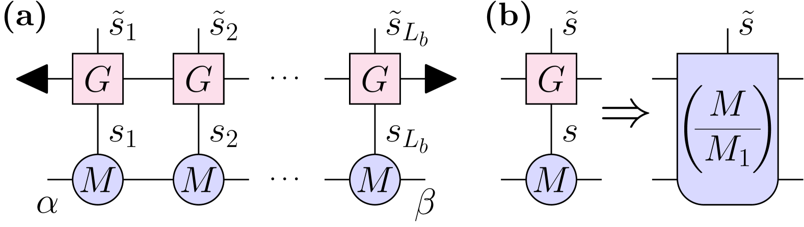
Figure 1: Action of MPO representation of $H_{1}$ on MPS $\ket{\psi}$. (a) Initial tensor network. (b) Contraction of inner physical indices.

For the $W$-state, we have $M^{0}=M_{1}^{1}=\begin{pmatrix}1\end{pmatrix}$, $M^{1}=M_{1}^{0}=\begin{pmatrix}0\end{pmatrix}$ and $B_{\alpha\beta}=\begin{pmatrix}1\end{pmatrix}$ giving

$$\left(\hskip-3.0pt\begin{array}[]{c}M\\ \hline\cr M_{1}\end{array}\hskip-3.0pt\right)^{0}=\begin{pmatrix}1&0\\ 0&1\end{pmatrix},\left(\hskip-3.0pt\begin{array}[]{c}M\\ \hline\cr M_{1}\end{array}\hskip-3.0pt\right)^{1}=\begin{pmatrix}0&0\\ 1&0\end{pmatrix},\mathcal{T}=\begin{pmatrix}0&1\\ 0&0\end{pmatrix},$$ (14)

which recovers the state’s bulk MPS commonly used with OBC terminations to compensate for the absence of an adequate TI MPS representation.

When $\ket{\psi}$ is a state with PBCs, $B_{\alpha\beta}=\delta_{\alpha\beta}$ and the construction of Eq. (12) is manifestly TI since it represents the action of a TI Hamiltonian on a TI state. This means that the position of $\mathcal{T}$ is irrelevant or,

$$\Tr{\mathcal{T}\left(\hskip-3.0pt\begin{array}[]{c}M\\ \hline\cr M_{1}\end{array}\hskip-3.0pt\right)^{s_{1}}\left(\hskip-3.0pt\begin{array}[]{c}M\\ \hline\cr M_{1}\end{array}\hskip-3.0pt\right)^{s_{2}}\cdots\left(\hskip-3.0pt\begin{array}[]{c}M\\ \hline\cr M_{1}\end{array}\hskip-3.0pt\right)^{s_{L_{b}}}}$$ (15)

$$=\Tr{\mathcal{T}\left(\hskip-3.0pt\begin{array}[]{c}M\\ \hline\cr M_{1}\end{array}\hskip-3.0pt\right)^{s_{L_{b}}}\left(\hskip-3.0pt\begin{array}[]{c}M\\ \hline\cr M_{1}\end{array}\hskip-3.0pt\right)^{s_{1}}\cdots\left(\hskip-3.0pt\begin{array}[]{c}M\\ \hline\cr M_{1}\end{array}\hskip-3.0pt\right)^{s_{L_{b}-1}}},$$

and so on. In fact, if we drop the requirement that the tensor $M_{1}$ represents the action of some operator on the physical index of tensor $M$ and assume the former to be completely arbitrary, or even assume inhomogeneous site-dependent tensors of the form given in Eq. (11), the cyclic property like that in Eq. (15) will still hold, which can readily be verified by a direct calculation using the identity

$$\left(\hskip-3.0pt\begin{array}[]{c}A\\ \hline\cr A_{1}\end{array}\hskip-3.0pt\right)^{s_{1}}\left(\hskip-3.0pt\begin{array}[]{c}B\\ \hline\cr B_{1}\end{array}\hskip-3.0pt\right)^{s_{2}}=\left(\hskip-3.0pt\begin{array}[]{c}AB\\ \hline\cr A_{1}B+AB_{1}\end{array}\hskip-3.0pt\right)^{s_{1}s_{2}}.$$ (16)

With this in mind, to emphasize the translational invariance of the construction, let us define the (homogeneous) TTI MPS representation of a state $\ket{\psi^{\prime}}$ in terms of the “twisted” trace operator $\operatorname{{\mathcal{T}\!\!\raisebox{-0.4pt}{\it tr}}\hskip-0.6pt}\left\{[\cdots]\right\}\equiv\Tr{\mathcal{T}[\cdots]}$ and two arbitrary tensors $M$ and $M_{1}$ of the same shape as follows:

$$\ket{\psi^{\prime}}=\sum_{\{s_{i}\}} \operatorname{{\mathcal{T}\!\!\raisebox{-0.4pt}{\it tr}}\hskip-0.6pt}\left\{\left(\hskip-3.0pt\begin{array}[]{c}M\\ \hline\cr M_{1}\end{array}\hskip-3.0pt\right)^{s_{1}}\left(\hskip-3.0pt\begin{array}[]{c}M\\ \hline\cr M_{1}\end{array}\hskip-3.0pt\right)^{s_{2}}\cdots\left(\hskip-3.0pt\begin{array}[]{c}M\\ \hline\cr M_{1}\end{array}\hskip-3.0pt\right)^{s_{L_{b}}}\right\}$$ (17)

$$\times\ket{s_{1}s_{2}\dots s_{L_{b}}}.$$

Our TTI MPS framework is, effectively, a more analytically convenient variant of the MPS “single-mode approximation” (SMA) used as a variational ansatz in Refs. [Haegeman_2012, Haegeman_2013, lin2019exact]. The primary advantage of the TTI MPS formulation over the traditional SMA is its close resemblance to the standard TI MPS form. This similarity allows us to apply the extensive toolset developed for TI MPS to TTI MPSs with only slight modifications. Clearly, any state that has a finite-bond-dimension TI MPS representation can trivially be expressed as a TTI MPS; the converse, however, is generically not true (e.g., the $W$-state). In this sense, the TTI MPS can be seen as an extension of the TI MPS. In App. LABEL:app:ground, we present several demonstrations of the analytical merits of the TTI MPS form, along with additional insights into the quasi-particle models discussed in Refs. [Omiya_2023quantum, Chandran_2023].

IV New exact $E=0$ MPS scars in the PXP and PPXPP models

((a))

((b))

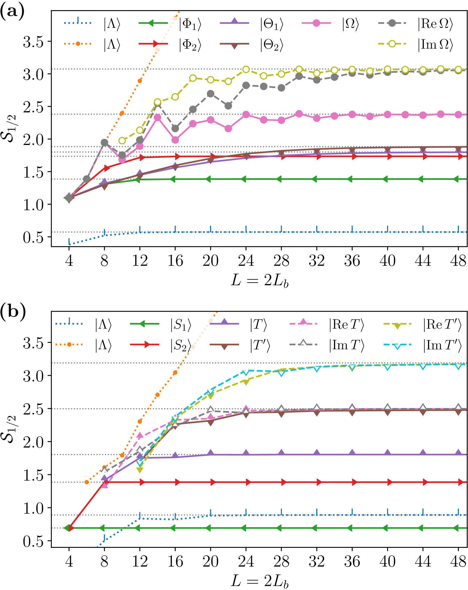
Figure 2: Dependence of bipartite entanglement entropy on the system size in (a) the PXP and (b) the PPXPP models. For each state, the system sizes are chosen such that both half-systems contain an integer number of local basis blocks. We plot two characteristic entanglement entropies of the maximally entangled (with respect to its standard bipartition) volume-law zero energy eigenstate $\ket{\Lambda}$ found in Ref. [Ivanov_2025], which for the two systems is defined on the appropriate constrained Hilbert space. The entanglement entropy of $\ket{\Lambda}$ with respect to the standard bipartition, essentially, continues growing linearly at the rate shown, whereas the entropy with respect to the entanglement minimizing bipartition quickly saturates at a low value. The increasing saturation values of the entanglement entropy of the consecutively introduced area-law states reflect a certain “complexity hierarchy” among them. Note also that saturation of the entanglement entropy for the new states introduced in this work typically occurs in significantly larger systems than that for the previously known states.

In this section, for easy reference, we will list the MPS representations of all currently known eigenstates of the PXP and PPXPP Hamiltonians with PBC. We will mark the states that have never appeared in the literature before as “new.” For the states first introduced in other works (not necessarily as MPSs) we will provide a reference to the original paper.

All our new states will exhibit a more complex structure compared to the previously known ones. This can be seen in Fig. 2 where we show the dependence of the bipartite entanglement entropy on the system size for all the states included in this section: in both the PXP and PPXPP models, the previously known eigenstates are the three states with the lowest values of the saturation entanglement entropy.

Our naming convention for the new eigenstates will roughly adhere to that used in previous works. We will use subscripts, as in $\ket{\Phi_{2}}=T_{x}\ket{\Phi_{1}}$, to denote pairs of translational symmetry breaking states related by the single-site translation operator $T_{x}$. The volume-entangled states from Ref. [Ivanov_2025] (expressed using the BA TI MPS form) as $\ket{\Lambda}$. For the states in the TTI MPS form, we will use the “prime” symbol; for example $\ket{T^{\prime}}$ is a TTI MPS on top of the TI MPS representation of the state $\ket{T}$. Some of our states will be complex-valued, which means, given the real-valuedness of $H_{\text{PXP/PPXPP}}$, that their separate real and imaginary parts will themselves be linearly independent eigenstates.

IV.1 PXP model

The $E=0$ exact eigenstates of the PXP model with PBC are the following:

$$\begin{aligned} &\ket{\Lambda}\\ &\text{Ref.~\cite[cite]{[\@@bibref{Number}{Ivanov_2025}{}{}]}}\end{aligned}:\scalebox{0.85}{$\underbrace{\frac{1}{2}\begin{pmatrix}1&1\\ 1&1\end{pmatrix}}_{M^{00}},\,\underbrace{-2\begin{pmatrix}0&0\\ 1&0\end{pmatrix}}_{M^{11}},\,\underbrace{\begin{pmatrix}0&0\\ 0&0\end{pmatrix}}_{M^{01/10}}$};$$ (18a)

$$\begin{aligned} &\ket{\Phi_{1}}\\ &\text{Ref.~\cite[cite]{[\@@bibref{Number}{lin2019exact}{}{}]}}\end{aligned}:\scalebox{0.85}{$\underbrace{\begin{pmatrix}0&-1\\ 1&0\end{pmatrix}}_{M^{O}},\,\underbrace{\begin{pmatrix}0&0\\ 0&-\sqrt{2}\end{pmatrix}}_{M^{L}},\,\underbrace{\begin{pmatrix}\sqrt{2}&0\\ 0&0\end{pmatrix}}_{M^{R}};$}$$ (18b)

$$\begin{aligned} &\ket{\Phi_{2}}\\ &\text{Ref.~\cite[cite]{[\@@bibref{Number}{lin2019exact}{}{}]}}\end{aligned}:\scalebox{0.85}{$\underbrace{\begin{pmatrix}0&-1&0\\ 1&0&0\\ 0&0&0\end{pmatrix}}_{M^{O}},\,\underbrace{\begin{pmatrix}\sqrt{2}&0&0\\ 0&0&0\\ -\sqrt{2}&0&0\end{pmatrix}}_{M^{L}},\,\underbrace{\begin{pmatrix}-\sqrt{2}&0&-\sqrt{2}\\ 0&0&0\\ 0&0&0\end{pmatrix}}_{M^{R}};$}$$ (18c)

$$\begin{aligned} &\bf\ket{\Theta_{1}}\\ &\textbf{new}\end{aligned}:\scalebox{0.85}{$\underbrace{\begin{pmatrix}0&3&-1&0\\ -1&0&0&1\\ 2&0&0&-6\\ 0&0&0&0\end{pmatrix}}_{M^{O}},\,\underbrace{\begin{pmatrix}0&0&0&0\\ 0&0&0&0\\ 0&3&-1&0\\ 1&0&0&-3\end{pmatrix}}_{M^{L}},\,\underbrace{\begin{pmatrix}1&0&0&0\\ 0&3&0&0\\ 0&0&0&0\\ 0&0&0&0\end{pmatrix}}_{M^{R}};\hskip-20.00003pt$}$$ (18d)

$$\begin{aligned} &\bf\ket{\Theta_{2}}\\ &\textbf{new}\end{aligned}:\scalebox{0.85}{$\underbrace{\begin{pmatrix}0&3&-1&0\\ -\frac{5}{3}&0&0&3\\ 0&0&0&0\\ 0&0&0&0\end{pmatrix}}_{M^{O}},\,\underbrace{\begin{pmatrix}\frac{9}{2}&0&0&-\frac{9}{2}\\ 0&0&0&0\\ 0&-3&1&0\\ \frac{3}{2}&0&0&-\frac{3}{2}\end{pmatrix}}_{M^{L}},\,\underbrace{\begin{pmatrix}0&0&0&0\\ 0&-1&0&0\\ 0&0&0&0\\ 1&0&0&-3\end{pmatrix}}_{M^{R}};\hskip-20.00003pt$}$$ (18e)

$$\begin{aligned} &\bf\ket{\Omega}\\ &\textbf{new}\end{aligned}:\scalebox{0.85}{$\underbrace{\begin{pmatrix}0&\frac{1}{8}&2&\frac{5}{6}\\ -8&-2&0&-2\\ -\frac{1}{2}&-\frac{1}{8}&0&-\frac{1}{8}\\ 0&\frac{1}{2}&8&-2\\ \end{pmatrix}}_{M^{0}},\,\underbrace{\frac{i}{\sqrt{3}}\begin{pmatrix}0&1&0&0\\ 0&0&0&0\\ 0&0&0&1\\ 0&0&0&0\\ \end{pmatrix}}_{M^{1}}$}.$$ (18f)

Note that $\ket{\Omega}$ is the first reported exact eigenstate (comprised of two orthogonal eigenstates $\ket{\real\Omega}$ and $\ket{\imaginary\Omega}$) that is defined for both even- and odd-length PBC chains.

Some of the basic properties of the states in Eqs. (18a)–(18f) — such as $T_{x}$, $\mathcal{C}$, and $\mathcal{I}$ symmetry quantum numbers, the saturation values of the bipartite entanglement entropy $\lim_{L\to\infty}\mathcal{S}_{1/2}$ [cf. Fig. 2(a)], and correlation lengths $\xi$ — are given in Table 1. The instances where the correlation length is defined correspond to injective MPSs. Derivations of these and some additional properties (such as norms and various overlaps) are available in Apps. LABEL:app:propspxp and LABEL:app:entpxp.

Table 1: Properties of the $E=0$ eigenstates of $H_{\text{PXP}}$.

State	$T_{x}$	$\mathcal{C}$, $\mathcal{I}$	$\lim_{L\to\infty}\mathcal{S}_{1/2}$	$\xi$
$\ket{\Lambda}$	$+1$	$+1$	$\sim 0.5895$	$\sim 1.0390$
$\ket{\Phi_{1}}$	—	$(-1)^{L_{b}}$	$2\log 2$	$\sim 1.8205$
$\ket{\Phi_{2}}$	—	$(-1)^{L_{b}}$	$2\log(3/2^{1/3})$	$\sim 1.8205$
$\ket{\Theta_{1}}$	—	$(-1)^{L_{b}}$	$\sim 1.8010$	$\sim 6.9834$
$\ket{\Theta_{2}}$	—	$(-1)^{L_{b}}$	$\sim 1.8839$	$\sim 6.9834$
$\ket{\Omega}$	$+1$	—	$\sim 2.3811$	$\sim 7.9294$
$\ket{\real\Omega}$	$+1$	$+1$	$\mathcal{S}^{\ket{\Omega}}_{1/2}+\log 2$	—
$\ket{\imaginary\Omega}$	$+1$	$-1$	$\mathcal{S}^{\ket{\Omega}}_{1/2}+\log 2$	—

IV.2 PPXPP model

The $E=0$ exact eigenstates of the PPXPP model with PBC that are representable as TI MPSs are the following:

$$\begin{aligned} &\ket{\Lambda}\\ &\text{Ref.~\cite[cite]{[\@@bibref{Number}{Ivanov_2025}{}{}]}}\end{aligned}:\scalebox{0.85}{$\underbrace{\begin{pmatrix}0&0&1\\ 0&0&-1\\ 1&1&1\end{pmatrix}}_{M^{00}},\,\underbrace{\begin{pmatrix}0&0&0\\ -1&0&0\\ 0&0&0\end{pmatrix}}_{M^{11}},\,\underbrace{\begin{pmatrix}0&0&0\\ 0&0&0\\ 0&0&0\end{pmatrix}}_{M^{01/10}};$}$$ (19a)

$$\begin{aligned} &\ket{S_{1}}\\ &\text{Ref.~\cite[cite]{[\@@bibref{Number}{Surace_2021}{}{}]}}\end{aligned}:\scalebox{0.85}{$\underbrace{\begin{pmatrix}0&1\\ 0&0\end{pmatrix}}_{M^{O}},\,\underbrace{\begin{pmatrix}0&0\\ -1&0\end{pmatrix}}_{M^{L}},\,\underbrace{\begin{pmatrix}0&0\\ 1&0\end{pmatrix}}_{M^{R}}$};$$ (19b)

$$\begin{aligned} &\ket{S_{2}}\\ &\text{Ref.~\cite[cite]{[\@@bibref{Number}{Surace_2021}{}{}]}}\end{aligned}:\scalebox{0.85}{$\underbrace{\begin{pmatrix}0&1&0\\ 0&0&1\\ 0&0&0\end{pmatrix}}_{M^{O}},\,\underbrace{\begin{pmatrix}0&0&0\\ 0&0&0\\ 0&1&0\end{pmatrix}}_{M^{L}},\,\underbrace{\begin{pmatrix}0&0&0\\ -1&0&0\\ 0&0&0\end{pmatrix}}_{M^{R}}$};$$ (19c)

$$\begin{aligned} &\bf\ket{T}\\ &\textbf{new}\end{aligned}:\scalebox{0.85}{$\underbrace{\begin{pmatrix}1&0&\gamma^{*}-1\\ 0&\gamma&0\\ 1&0&\gamma^{*}-1\end{pmatrix}}_{M^{O}},\,\underbrace{\begin{pmatrix}0&1&0\\ 0&0&0\\ 0&0&0\end{pmatrix}}_{M^{L}},\,\underbrace{\begin{pmatrix}\ 0&0&0\\ 0&0&1\\ 0&0&0\end{pmatrix}}_{M^{R}}$};$$ (19d)

$$\begin{aligned} &\bf\ket{S^{\prime}_{1}}\\ &\textbf{new}\end{aligned}:\scalebox{0.85}{$\underbrace{\begin{pmatrix}1&1\\ 0&0\end{pmatrix}}_{M_{1}^{O}},\,\underbrace{\begin{pmatrix}0&0\\ 0&0\end{pmatrix}}_{M_{1}^{L}},\,\underbrace{\begin{pmatrix}0&0\\ 0&0\end{pmatrix}}_{M_{1}^{R}}$};$$ (19e)

$$\begin{aligned} &\bf\ket{S^{\prime}_{2}}\\ &\textbf{new}\end{aligned}:\scalebox{0.85}{$\underbrace{\begin{pmatrix}0&1&0\\ 0&1&1\\ 0&0&0\end{pmatrix}}_{M_{1}^{O}},\,\underbrace{\begin{pmatrix}0&0&0\\ 0&0&0\\ 0&0&0\end{pmatrix}}_{M_{1}^{L}},\,\underbrace{\begin{pmatrix}0&0&0\\ 0&0&0\\ 0&0&0\end{pmatrix}}_{M_{1}^{R}}$};$$ (19f)

$$\begin{aligned} &\bf\ket{T^{\prime}}\\ &\textbf{new}\end{aligned}:\scalebox{0.85}{$\underbrace{\begin{pmatrix}0&\gamma^{*}-1&0\\ 1&0&-1\\ 0&-1&0\end{pmatrix}}_{M_{1}^{O}},\,\underbrace{\begin{pmatrix}0&0&1\\ 0&0&0\\ 0&0&0\end{pmatrix}}_{M_{1}^{L}},\,\underbrace{\begin{pmatrix}0&0&-1\\ 0&0&0\\ 0&0&0\end{pmatrix}}_{M_{1}^{R}}$}.$$ (19g)

Here $\gamma=2^{-1/6}e^{\pm i\pi/4}$; the two choices for $\gamma$ generate two linearly independent, but not orthogonal, states related by complex conjugation.

While all the MPSs representing the known eigenstates of the PXP model listed in Eqs. (18a)–(18f) are injective, which suggests that they are native to the bases they are expressed in, this is not the case for some of the MPSs in Eqs. (19a)–(19d) — here, we do not consider the TTI MPSs, whose bulk tensors are non-injective by construction. Specifically, only the representations of $\ket{\Lambda}$ in Eq. (19a) and $\ket{T}$ in Eq. (19d) are injective MPSs, whereas those of $\ket{S_{1}}$ and $\ket{S_{2}}$ in Eqs. (19b) and (19c) are not. It is easy to see that the state $\ket{S_{1}}$ is a $T_{x}^{2}$-invariant version of the state

$$\ket{\phi_{2}}=\bigotimes_{i_{b}=1}^{L_{b}/2}[\ket{R}-\ket{L}]_{2i_{b}-1}\otimes\ket{O}_{2i_{b}},$$ (20)

first reported in Ref. [Surace_2021], which means that when $L_{b}$ is even there exists a $p$-periodic (with $p=2$ blocks) decomposition of $\ket{S_{1}}$ into two injective MPSs with bond dimension 1, whereas when $L_{b}$ is odd $\ket{S_{1}}$ vanishes [perez2007matrix]. Similarly, $\ket{S_{2}}$ is decomposable into injective MPSs with bond dimensions $1$ and $2$ when $L_{b}$ is even, and when $L_{b}$ is odd $\ket{S_{2}}=0$. In Sec. LABEL:sec:extrap_pxp_p, we will re-examine states such as $\ket{\phi_{2}}$ and other states from Ref. [Surace_2021] utilizing the framework to be introduced in Sec. V.

Surprisingly, TTI MPSs on top of the states $\ket{S_{1}}$ and $\ket{S_{2}}$ with the $M_{1}$ tensors given in Eqs. (19e) and (19f), respectively, generate previously unknown exact eigenstates $\ket{S^{\prime}_{1}}$ and $\ket{S^{\prime}_{2}}$ that do not vanish when $L_{b}$ is odd; when $L_{b}$ is even, $\ket{S^{\prime}_{1}}$ and $\ket{S^{\prime}_{2}}$ are identical to, respectively, $\ket{S_{1}}$ and $\ket{S_{2}}$.

On the other hand, a TTI MPS $\ket{T^{\prime}}$ on top of the new state $\ket{T}$ generates a new complex-valued state which is different from $\ket{T}$ in all system sizes. This means that $\ket{T}$ and $\ket{T^{\prime}}$ together generate four new linearly independent eigenstates of $H_{\text{PPXPP}}$.

Table 2 summarizes the same set of basic properties for the eigenstates of the PPXPP in Eqs. (19b)–(19g) as those given in Table 1 for the eigenstates of the PXP model. As before, the instances where the correlation length is defined correspond to injective MPSs. Derivations of these and some additional properties (such as norms and various overlaps) were performed analogously to those in App. LABEL:app:propspxp.

Table 2: Properties of the $E=0$ eigenstates of $H_{\text{PPXPP}}$.

State	$T_{x}$	$\mathcal{C}$, $\mathcal{I}$	$\lim_{L\to\infty}\mathcal{S}_{1/2}$	$\xi$
$\ket{S_{1}}$, $\ket{S^{\prime}_{1}}$	—	$(-1)^{\left\lfloor\frac{L_{b}}{2}\right\rfloor}$	$\log 2$	—
$\ket{S_{2}}$, $\ket{S^{\prime}_{2}}$	—	$(-1)^{\left\lfloor\frac{L_{b}}{2}\right\rfloor}$	$2\log 2$	—
$\ket{\Lambda}$	$+1$	$+1$	$\sim 0.8900$	$\sim 1.7441$
$\ket{T}$	—	$+1$	$\sim 1.8035$	$\sim 3.4882$
$\ket{T^{\prime}}$	—	$-1$	$\mathcal{S}^{\ket{T}}_{1/2}+\log 2$	—
$\ket{\real T}$	$+1$	$+1$	$\mathcal{S}^{\ket{T}}_{1/2}+\log 2$	—
$\ket{\imaginary T}$	$-1$	$+1$	$\mathcal{S}^{\ket{T}}_{1/2}+\log 2$	—
$\ket{\real T^{\prime}}$	$-1$	$-1$	$\mathcal{S}^{\ket{T^{\prime}}}_{1/2}+\log 2$	—
$\ket{\imaginary T^{\prime}}$	$+1$	$-1$	$\mathcal{S}^{\ket{T^{\prime}}}_{1/2}+\log 2$	—

V Proofs

In the previous section we introduced several new $E=0$ eigenstates of the PXP and PPXPP chains with PBC without providing any proofs. Now, our objective is to develop a framework that allows for direct proofs of such $E=0$ eigenstates in kineticaly constrained models. This framework will provide a procedure for generating conditions based on the specific properties of a given Hamiltonian that are sufficient for an MPS to represent its exact zero energy eigenstate. Our approach is applicable to both the newly introduced and previously reported eigenstates of PXP-type models. This suggests that it should also be applicable to $E=0$ eigenstates of these models yet to be discovered.

For concreteness, let us start by revisiting the technique used in Ref. [lin2019exact] to prove the eigenstate $\ket{\Phi_{1}}$ of the PXP model in the context of the following two technical results (applicable for both PBC and OBC cases assuming an appropriate definition of the Fibonacci subspace $\mathcal{H}^{1}$):

Lemma 1.

Any $\ket{\psi}\in\mathcal{H}^{1}$ such that $H_{1}\ket{\psi}=\lambda\ket{\psi}$ is an exact eigenstate of $H_{\mathrm{PXP}}$ with energy $\lambda$.

Proof.

Let $\mathcal{P}_{f}$ be a projector onto the Fibonacci subspace. The condition that $\ket{\psi}\in\mathcal{H}^{1}$ is equivalent to $\mathcal{P}_{f}\ket{\psi}=\ket{\psi}$. Therefore, acting with $\mathcal{P}_{f}$ on both sides of the eigenvalue equation $H_{1}\ket{\psi}=\lambda\ket{\psi}$, we get $\mathcal{P}_{f}H_{1}\ket{\psi}=\lambda\ket{\psi}$. On the subspace $\mathcal{H}^{1}$, $H_{\text{PXP}}=\mathcal{P}_{f}H_{\text{PXP}}\mathcal{P}_{f}=\mathcal{P}_{f}H_{1}\mathcal{P}_{f}$, where we have used $\mathcal{P}_{f}H_{2}\mathcal{P}_{f}=0$ easily seen by inspection of individual terms in $H_{2}$. Therefore, $H_{\text{PXP}}\ket{\psi}=\mathcal{P}_{f}H_{1}\ket{\psi}=\lambda\ket{\psi}$. ∎

Corollary 1.1.

Any $\ket{\psi}\in\mathcal{H}^{1}$ such that $H_{1}\ket{\psi}=\lambda\ket{\psi}$ is annihilated by $H_{2}$ .

The proofs in Ref. [lin2019exact] establishing their state $\ket{\Phi_{1}}$ as an exact eigenstate of $H_{\text{PXP}}$ first explicitly checked that the state (residing in $\mathcal{H}^{1}$ by construction) was annihilated by $H_{2}$ and then showed that it was an exact eigenstate of $H_{1}$ with zero energy. Per Corollary 1.1, however, it would suffice to show only the latter. We state this not for the sake of pointing out that certain calculations were unnecessary, but rather to appreciate the fact that the approach used in Ref. [lin2019exact] to prove that an MPS defined on $\mathcal{H}^{1}$ is an exact eigenstate of $H_{1}$ can be generalized into a framework for proving (and potentially discovering) new exact eigenstates of $H_{\text{PXP}}$ satisfying the conditions of Lemma 1. We summarize such generalization in the following:

Theorem 2.

Suppose matrices $M^{s}$, $s\in\{O,L,R\}$ are an MPS representation of $\ket{\psi}\in\mathcal{H}^{1}$, satisfying

$$M^{R}M^{L}=\mathbf{0}.$$ (21)

In the case of PBC, where $M^{s}$ define a TI MPS, if there exists a matrix $X$ such that

$$[X,M^{O}]=F^{O},$$ (22a)

$$[X,M^{L}]=F^{L},$$ (22b)

$$[X,M^{R}]=F^{R},$$ (22c)

where

$$F^{O}=M^{L}+M^{R},\quad F^{L}=F^{R}=M^{O}~,$$ (23)

then $\ket{\psi}$ satisfies the conditions of Lemma 1 with $\lambda=0$ (i.e., is an exact zero energy eigenstate of $H_{\text{PXP}}$). In the case of OBC, if the terminations are chosen to be left and right eigenvectors $v^{T}$ and $w$ of $X$ with eigenvalues $\lambda_{v}$ and $\lambda_{w}$, then $\ket{\psi}$ satisfies the conditions of Lemma 1 with $\lambda=\lambda_{v}-\lambda_{w}$.

Proof.

The action of $H_{1}$ on $\ket{\psi}$ has the following TTI MPS representation:

$$H{}_1|\psi ⟩:\text{<div class="ltx\_inline-block ltx\_transformed\_outer" style="width:32.5pt;height:13.7pt;vertical-align:-2.1pt;"><span class="ltx\_transformed\_inner" style="transform:translate(-2.9pt,1.0pt) scale(0.85,0.85) ;"> <p class="ltx\_p">{</p> </span></div>}$$ (24)