Euclid Quick Data Release (Q1)

We present a detailed visual morphology catalogue for Euclid’s Quick Release 1 (Q1). Our catalogue includes galaxy features such as bars, spiral arms, and ongoing mergers, for the 378 000 bright ($I_{\scriptscriptstyle\rm E}<20.5$) or extended (area $\geq 700\,$pixels) galaxies in Q1. The catalogue was created by finetuning the Zoobot galaxy foundation models on annotations from an intensive one month campaign by Galaxy Zoo volunteers. Our measurements are fully automated and hence fully scaleable. This catalogue is the first 0.4% of the approximately 100 million galaxies where Euclid will ultimately resolve detailed morphology.

1 Introduction

Detailed visual morphology refers to the recognizable features which comprise a galaxy, such as bars, spiral arms, and tidal tails (Hubble 1926; De Vaucouleurs 1959; Toomre1972; sellwoodSpiralsGalaxies2022). Understanding how galaxies acquire their stellar structure provides key insights into the processes driving mass assembly in the Universe (e.g. 2011ApJ...742...96W; 2015Sci...348..314T; Huertas-Company et al. 2016) Visual morphology has historically also described the method of detection; we measure these features visually, by eye. Those eyes may either belong to professional astronomers (Nair & Abraham 2010; Baillard et al. 2011; Buta et al. 2015) or to members of the public taking part in citizen science projects such as Galaxy Zoo (Lintott et al. 2008; Masters 2019) and Galaxy Cruise (tanaka_galaxy_2023). Visual morphology complements parametric morphology, such as Sérsic fitting (sersic_influence_1963), and non-parametric morphology, such as concentration and asymmetry (Morgan 1958; Conselice et al. 2000; shimasaku_statistical_2001; Abraham et al. 2003), which both use rule-based automated methods to interpret galaxy images. Parametric and non-parametric morphology have historically been together known as ‘quantitative’ morphology, contrasting with ‘qualitative’ visual morphology.

The complexity of galaxies is greater than the complexity we are able to express in code. Galaxies have features which are too complex for our rule-based methods, but are real nonetheless (see e.g., Lintott et al. 2009; Rudnick2021; Bowles et al. 2023; Gordon et al. 2024). Astronomers have therefore faced a trade-off. One can use visual morphology to capture detailed features, or quantitive morphology to make measurements which are scaleable and reproducible (Conselice 2014). There is also a spectrum of work between these two extremes that makes detailed automated measurements under a degree of manual supervision and tuning, e.g., galfit (peng_detailed_2002) and Galaxy Zoo Builder (Lingard et al. 2020).

Recent advances in computer vision make it possible, even straightforward, to automate some visual judgements. Seminal work by Dieleman et al. (2015) won the Galaxy Challenge, a Kaggle competition to predict the visual judgements of Galaxy Zoo volunteers, and in doing so introduced deep learning to astronomy. A decade later, deep learning is a ubiquitous tool for measuring visual morphology (e.g., Khan et al. 2019; Abraham et al. 2018; Pearson2019Mergers; Ghosh et al. 2020; Bom et al. 2021; ciprijanovic_semi-supervised_2022 and review by Huertas-Company & Lanusse 2023). Citizen science and deep learning have together underpinned detailed visual morphology catalogues for the Hubble Space Telescope (Huertas-Company et al. 2015), the Sloan Digital Sky Survey (Domnguez Snchez et al. 2018), the Dark Energy Camera Legacy Survey (Walmsley2022decals), and the companion Legacy Surveys (walmsleyGalaxyZooDESI2023; yeGalaxyZooDECaLS2025).

Our core advance here is timing. Morphology catalogues typically follow years after a telescope data release – 3.5 to 5 years for each of Galaxy Zoo’s morphology catalogues, for example. Much of this time is needed for volunteers to annotate galaxies and, more recently, to train models.

What if we made morphology measurements at the same time as the survey takes images, just as we already do for other automated measurements? Placing a trained deep learning model within the survey image processing pipeline allows for immediate morphology measurements and immediate use by scientists. Our models can be trained quickly because we use new ‘foundation’ models (described in Sect. 3.2) that need fewer examples to learn to classify new surveys. In this work, we deliver a detailed visual morphology catalogue for Euclid in weeks instead of years.

Euclid will resolve the detailed visual morphology of at least an order of magnitude more galaxies than have ever been measured. The largest current detailed morphology catalogues use images from the DESI Legacy Surveys (walmsleyGalaxyZooDESI2023), with 19 000 deg² of imaging at $1.\mathrm{″}1$ seeing; and the Sloan Digital Sky Survey (Willett2013; Domnguez Snchez et al. 2018), with 9000 deg² of imaging at $1.\mathrm{″}3$ seeing (DR7, Abazajian et al. 2009). The EWS will cover approximately 14 000 deg² with a spatial resolution of $0.\mathrm{″}16$ (Euclid Collaboration: Cropper et al. 2024) – a comparable area at ten times higher resolution. The final Euclid morphology catalogues will include approximately $10^{8}$ galaxies. Here, we measure detailed morphology in the first 0.4% – Euclid Quick Release 1 (Q1, Euclid Quick Release Q1 2025).

Euclid connects low-redshift ground-based morphology measurements with high-redshift space-based measurements, enabling a continuous view of galaxy morphology through time. Figure 1 compares, as a function of redshift, the number of galaxies with visual features in our Q1 catalogue vs. previous catalogues made with the Sloan Digital Sky Survey (Willett2013), the Hubble Space Telescope (HST, Willett2017a), and the Legacy Surveys (walmsleyGalaxyZooDESI2023). Q1 adds an order-of-magnitude more galaxies between $0.3<z<0.7$. Straightforwardly multiplying our results by area, the EWS will ultimately increase the number of galaxies with measured morphology features between $0.3<z<0.7$ by around three orders of magnitude.

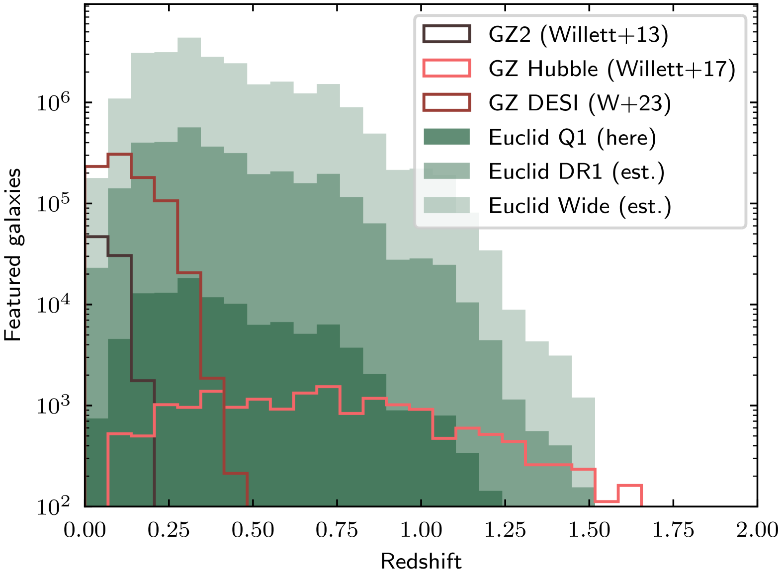
Figure 1: Galaxies with well-resolved features as a function of redshift, for morphology catalogues from Euclid vs. Galaxy Zoo 2 (main sample, Willett2013), Galaxy Zoo Hubble (Willett2017a), and Galaxy Zoo DESI (walmsleyGalaxyZooDESI2023). Euclid will outscale all current visual morphology catalogues for all redshifts below $z<1.5$, typically by several orders of magnitude. Q1 morphologies may be especially valuable between $0.3<z<0.7$. We define ‘featured’ as a galaxy with an expected volunteer vote fraction for ‘Featured’ above 0.5 (see Sect. 5). ‘Euclid Q1’ is this catalogue; estimates for ‘Euclid DR1’ and ‘Euclid Wide’ (EWS) are made by trivially multiplying our catalogue counts by area. Euclid redshifts are photometric (Euclid Collaboration: Tucci et al. 2025).

Our Q1 catalogue is available in two forms. First, our initial trained model is part of the Euclid pipeline, and so the morphology measurements from that model are reported as part of the Q1 data release (Euclid Collaboration: Romelli et al. 2025). Those measurements are accessible through the ESA Science Archive Service as with other core measurements such as photometry, redshifts, and so forth. We refer to this as the pipeline catalogue. Second, we created a separate catalogue by applying our next generation of models directly to the Euclid images, outside of the Euclid pipeline. We did this to use the best possible models (which are updated more frequently than is practical within the Euclid pipeline) and to create and share our embeddings (vectors which mathematically summarise the visual features of each galaxy). We refer to this as the dynamic catalogue.

Our catalogue complements parallel work by Euclid Collaboration: Romelli et al. (2025) and Euclid Collaboration: Quilley et al. (2025) to create a morphology catalogue for Q1 with parametric and non-parametric measurements. We recommend using these traditional measurements for galaxies less extended than around 700 pixels in segmentation area, below which Euclid cannot reliably resolve detailed features. Euclid Collaboration: Quilley et al. (2025) includes a comparison of disk and bulge measurements using this detailed morphology catalogue and using Sérsic fits and finds consistent results.

Our catalogue was made possible by the efforts of 9976 Galaxy Zoo volunteers who together contributed 2.9M annotations to adapt the Zoobot foundation deep learning models for Euclid images. These measurements, combined with parallel work using the Zoobot models to find strong lenses (Euclid Collaboration: Walmsley et al. 2025; Euclid Collaboration: Rojas et al. 2025; Euclid Collaboration: Lines et al. 2025; Euclid Collaboration: Li et al. 2025; Euclid Collaboration: Holloway et al. 2025), stellar bars (Euclid Collaboration: Huertas-Company et al. 2025), mergers (Euclid Collaboration: La Marca et al. 2025) and AGN (Euclid Collaboration: Margalef-Bentabol et al. 2025) demonstrate the practical value of foundation models in astronomy.

In Sect. 2, we describe our selection function and image processing choices. In Sect. 3.1, we describe how Galaxy Zoo volunteers contributed annotations. In Sect. 3.2, we motivate our use of foundation models and detail the finetuning process. In Sect. 4, we validate the performance of our finetuned models. In Sect. 5, we share our dynamic catalogue, embeddings, and images, and provide practical guidance on how these might be used. They can be downloaded from Zenodo and HuggingFace.

2 Data

2.1 Coverage

Euclid will detect approximately 1.5 billion sources (Euclid Collaboration: Bretonnière et al. 2022; Euclid Collaboration: Mellier et al. 2024). The largest sources will be revealed in exquisite detail (Hunt et al. 2024). Most will be barely resolved. In between will be a middle ground of sources which show some suggestion of detailed morphology (the trace of a disc, an arm, a bar, etc.). When choosing which galaxies to measure for detailed morphology, where should we draw the line?

The human annotations guiding the models that, in turn, create our catalogue, come from Galaxy Zoo volunteers – members of the public contributing their time to click through galaxy images (Masters 2019). We need to make the best possible use of Galaxy Zoo volunteers’ time, particularly during the one month labelling campaign to produce the pipeline models (Sect. 3.1). We should especially avoid showing a high ratio of featureless galaxies (‘blobs’) as these are relatively straightforward to classify automatically and may dissuade volunteers. Therefore, we chose the following conservative cut to select galaxies with a moderate chance of showing detailed features.

segmentation_area $>1200$ pixels

OR $I_{\scriptscriptstyle\rm E}<20.5$ AND segmentation_area$>200$ pixels

We found segmentation area (the total number of pixels within the segmentation source mask from SourceExtractor++, as calculated by Euclid Collaboration: Romelli et al. 2025) to be the critical factor in determining if a galaxy was well-resolved. Segmentation area is a natural proxy for assessing if a galaxy is well-resolved because each morphological feature requires sampling by some number of point spread function full-width-half-maximum (FWHM) to be resolved, and this sampling happens in two dimensions. Results using radii were broadly similar but suffered from orientation effects or asymmetric sources. Our choice of 1200 pixels was a subjective choice with the aim of creating an engaging sample for Galaxy Zoo volunteers (see above), and was ultimately later revised for the dynamic catalogue (below). The magnitude cut follows from the common science requirement for completeness, and is complemented by an alternative (far more generous) segmentation cut to remove galaxies where detailed features are plainly unmeasurable. Overall, this selection cut includes the brightest and most extended 0.8% of galaxies in Q1 ($195\,716$ galaxies). These form the selection shown to volunteers and measured by the pipeline models.

For the dynamic catalogue, we reduce the segmentation_area cut from $1200$ pixels to $700$ pixels (for a total of $380\,111$ galaxies, 1.5% of Q1). This adds $184\,395$ galaxies which are fainter and less extended but may still have resolvable features. We do not (currently) show these less extended galaxies to Galaxy Zoo volunteers, and instead rely on our trained models to extrapolate to this regime. The dynamic catalogue includes the column ‘in_extrapolated_selection’ for users to include or exclude these additional galaxies as desired. Lacking ground truth labels, we cannot make any performance claim for these galaxies, but our expert visual inspection qualitatively suggests the models continue to work similarly well – perhaps because the images are less detailed and therefore present a less challenging computer vision task, because the segmentation area is imprecisely measured, or because the models were pretrained on similar images from other surveys (walmsleyScalingLawsGalaxy2024).

While we could make automated measurements of every source in Q1, visually inspecting example images suggested that galaxies with a segmentation area below around 700 pixels are insufficiently resolved to clearly show detailed features, and so we select our lowest area cut as 700 pixels and defer deep learning morphology measurements of smaller galaxies to future work. Figure 2 illustrates our choice of selection cuts.

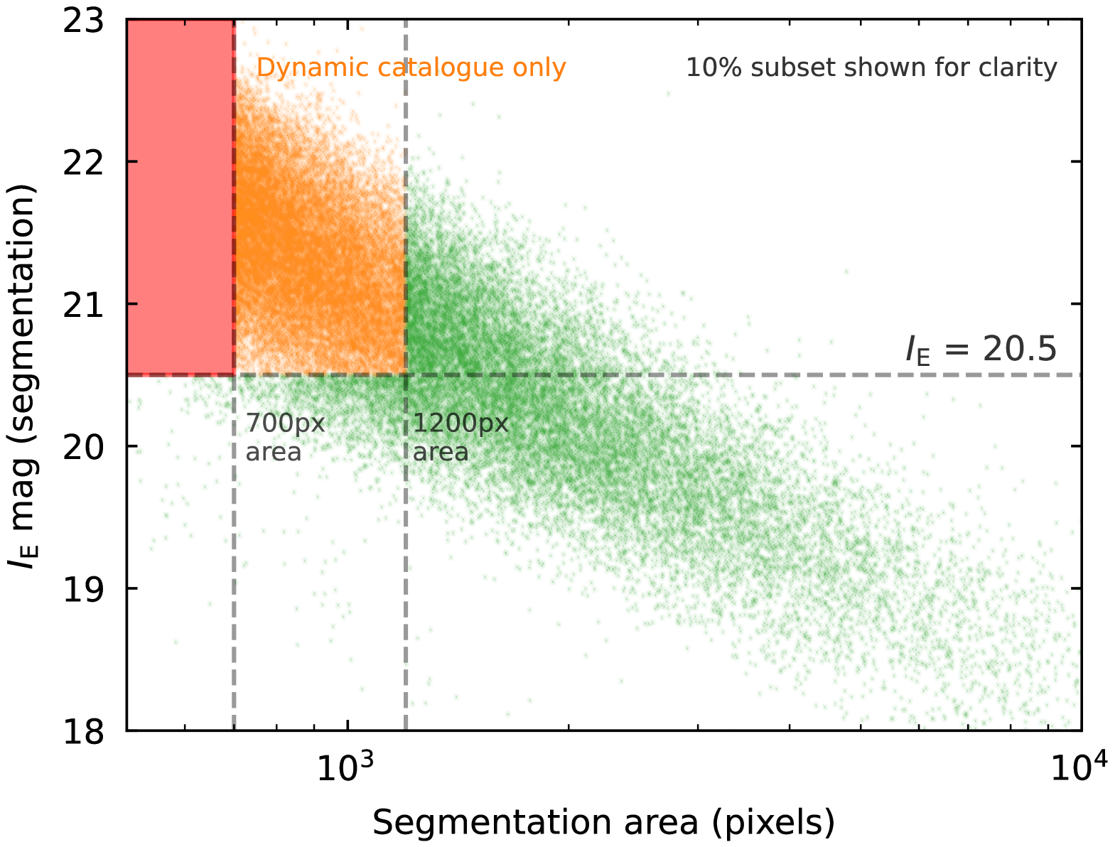
Figure 2: Cuts applied to select galaxies with resolvable visual morphology. The pipeline catalogue includes all galaxies with area ¿ 1200 pixels or $I_{\scriptscriptstyle\rm E}$ ¡ 20.5 (and area ¿ 200 pixels). The dynamic catalogue reduces the area limit to 700 pixels. The total number of galaxies in the dynamic catalogue only (orange) vs. in both catalogues (green) are roughly equal ($195\,716$ vs. $184\,395$, respectively)

For both selections, we additionally require vis_det$=1$ and spurious_prob$<0.2$, to remove artifacts, and require no Gaia cross-match to remove stars.

2.2 Image processing

We create three jpg cutouts from each source. Figure 3 shows examples. The three cutouts are:

1. A composite RGB image where the R channel is $Y_{\scriptscriptstyle\rm E}$, the B channel is $I_{\scriptscriptstyle\rm E}$, and the G channel is the mean of the pixelwise flux in the other two channels, following a 99.85th percentile clip and an arcsinh stretch, i.e., $x^{\prime}=$ arcsinh$(Qx)$ with $Q=100$ where $x$ is the flux in each pixel.

2. A greyscale image where the single channel is identical to the $I_{\scriptscriptstyle\rm E}$/B channel above, maximising resolution

3. A greyscale image where the single channel is again from $I_{\scriptscriptstyle\rm E}$, but adjusted to highlight low-surface brightness features. We use the recipe from Gordon et al. (2024) with a stretch of 20 and a power of 0.5, and add a 98th percentile clip.

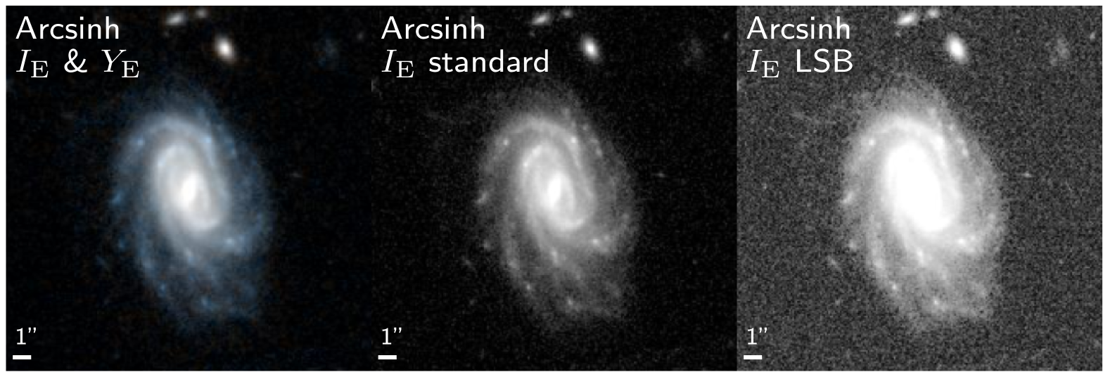
Figure 3: Example cutouts shown to volunteers. Left to right: $I_{\scriptscriptstyle\rm E}$/$Y_{\scriptscriptstyle\rm E}$ composite, $I_{\scriptscriptstyle\rm E}$-only greyscale with standard processing, $I_{\scriptscriptstyle\rm E}$-only greyscale with enhanced low-surface-brightness processing.

We designed these processing options to create a complementary set of images for volunteers; a colour image showing the general galaxy features, a maximum-sharpness (but greyscale) image, and an image aimed at highlighting low-surface brightness features which are better revealed when shown on a separate scale to the bright galaxy core. We used $Y_{\scriptscriptstyle\rm E}$ for the colour image as $Y_{\scriptscriptstyle\rm E}$ is the sharpest (lowest PSF FWHM) NISP band. We combined data from different instruments using the aligned and resampled mosaics provided by the MERge pipeline (Euclid Collaboration: Romelli et al. 2025).

Volunteers were shown all three images in a flipbook format with the order above. We then use their responses to adapt our models. The pipeline catalogue is made by a model shown the standard $I_{\scriptscriptstyle\rm E}$ image (only $I_{\scriptscriptstyle\rm E}$ is available). The dynamic catalogue is made by a model shown the composite $I_{\scriptscriptstyle\rm E}$/$Y_{\scriptscriptstyle\rm E}$ image.

3 Methods

3.1 Citizen science

We presented Euclid images to Galaxy Zoo volunteers. Volunteers annotated images from the Euclid Wide Survey (EWS), and not from Q1. Our pipeline models run within the Euclid pipeline that produced the Q1 data release, and so the pipeline models needed to be ready before Q1 was available. We showed these EWS images with permission from ESA and via a Memorandum of Understanding between the Euclid Consortium and the Zooniverse. This MoU created a framework for the Galaxy Zoo team to work with Euclid scientists to share a small set of EWS images with the public. These images are ideal for training models that work well on the EWS, and therefore on the vast majority of galaxies Euclid will image. We plan on returning to specifically annotate the Euclid Deep fields (including the Q1 area) once full-depth data is available.

The Euclid survey images are available as mosaic tiles of $$$\times$$$ (Euclid Collaboration: Romelli et al. 2025). Galaxies were selected from a set of tiles spread uniformly across the EWS area. All tiles were drawn from the southern half of the EWS (declination $<0$) as source catalogue data were not yet available for the northern half.

9976 volunteers contributed 2.9 million annotations of $114\,000$ galaxies. Of those, 1.56 million annotations were made in the initial one month labelling campaign and used to train the pipeline model. All 2.9 million annotations were used to train the dynamic catalogue model.

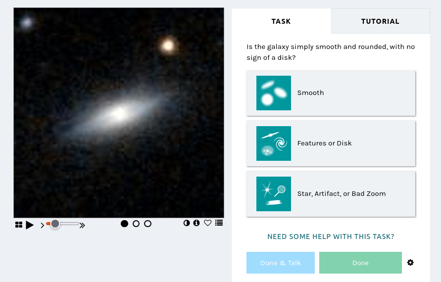
Figure 4: Galaxy Zoo annotation interface, as shown to volunteers. Volunteers answer a tree of questions, where the next question depends on the previous answer; only the first question is shown here.

Volunteers were presented with a pop-up tutorial, and shown examples in ‘help’ instructions for each question alongside a site-wide ‘field guide’. The annotation interface is shown in Fig. 4. In line with previous Galaxy Zoo projects, a small portion of highly-engaged volunteers contribute the bulk of the annotations. Volunteer contributions are well-modelled by a Pareto distribution (Fig. 5).

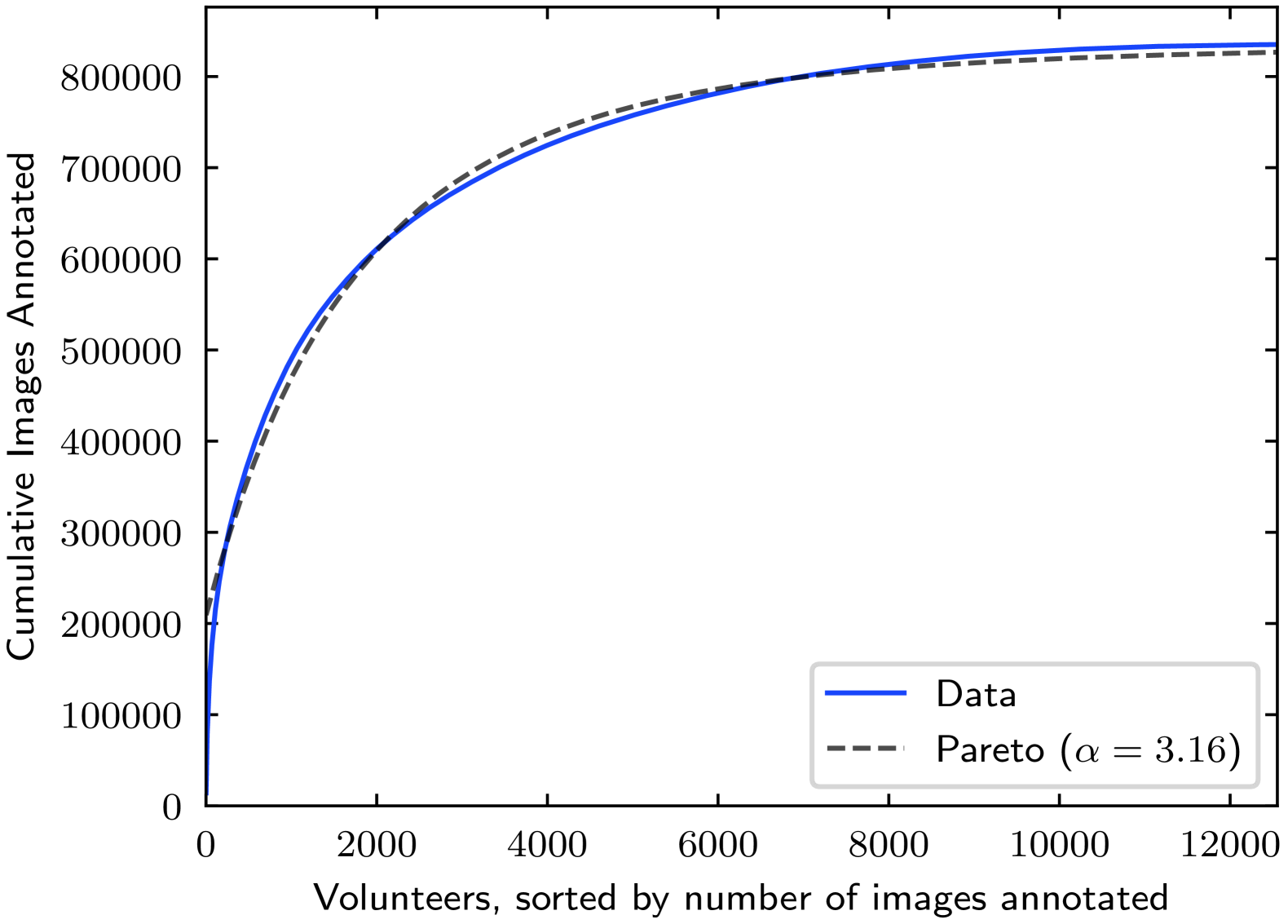
Figure 5: Cumulative images annotated when selecting the $N$ volunteers who annotated the most images. The bulk of annotations come from highly-engaged volunteers.

We decided to request five volunteer annotations per galaxy for the most galaxies ($110\,000$ of $114\,000$). Five volunteers is far fewer than typical; Galaxy Zoo has historically collected classifications from 40 volunteers per galaxy (for example Willett2013). Asking fewer volunteers per galaxy increases the noise in our labels but also increases the diversity of galaxies labelled. We hypothesize that this is a useful trade-off for maximising model performance provided the model loss function can handle uncertain labels (see Sect. 3.2). To accurately measure model performance, we also chose a small random subset ($3500$) to be annotated by 25 volunteers.

Maximising model performance is our key goal because only a tiny fraction of galaxies imaged by Euclid will ever be seen by humans. The complete EWS will include approximately $10^{8}$ galaxies passing our selection cuts above, compared to $\lesssim 2$M galaxies in all Galaxy Zoo projects over the last 15 years. It is impossible for volunteers to annotate more than a few percent of Euclid galaxies. We therefore do not expect scientists to use the volunteer annotations directly, as in all Galaxy Zoo projects prior to Walmsley2022decals, but instead to rely on model predictions. Collecting volunteer annotations to maximise model performance ultimately makes volunteers even more vital because we gain a multiplicative benefit from each annotation; a volunteer annotating one galaxy helps improve a model that annotates all galaxies.

3.2 Foundation models and finetuning

The models used here are the end result of a research project developing adaptable models for galaxy morphology. We briefly summarise the computer science motivation and previous progress below.

Transfer learning is the practice of training on one task to do better at a second task. Image features learned on the first task are hoped to ‘transfer’ (be relevant) to the second task (Lu et al. 2015). Transfer learning is especially useful where data for the second task is scarce. This was recognised early on as a useful technique in astronomy (Ackermann et al. 2018; Dominguez Sanchez et al. 2019; Tang2019).

Separately, models trained simultaneously on a diverse set of related tasks often outperform models trained on any single task (Caruana 1997). One explanation is that labels for one task can help models learn general image features relevant to other tasks. Earlier work in this project trained models on multiple morphology tasks in a single survey (Walmsley2022decals) and then expanded to training models on several closely related surveys (walmsleyGalaxyZooDESI2023).

Foundation models (Bommasani et al. 2021; Oquab et al. 2023) combine both transfer learning and multi-task learning. Foundation models involve two model-building phases: ‘pre-training’ on multiple tasks and then ‘downstream finetuning’ where the trained model is adapted to a new task. The hope is that the foundation model learns to extract generally useful image features (from multi-task learning) which are then applied to solve the new task (as in transfer learning). Walmsley2022practical found that the multi-survey pretrained model extracted features that were useful for similarity search (finding similar galaxies to a query galaxy), personalised anomaly recommendation (finding galaxies interesting to a specific user), and new morphology tasks. This motivated the release of Zoobot (Walmsley2023zoobot), the first galaxy foundation models designed to be adapted by other people to new galaxy image tasks. Zoobot is part of a recent trend towards foundation models in astronomy (rozanskiSpectralFoundationModel2023; Leung & Bovy 2023; Koblischke & Bovy 2024; parker_astroclip_2024). In related work, Euclid Collaboration: Siudek et al. (2025) experiments with applying the foundation model of smithAstroPTScalingLarge2024 to Q1.

Model ‘scaling laws’ (not to be confused with galaxy scaling laws) describe how model performance predictably increases when increasing any of one variable of data, training compute, or parameters, provided the other two variables are plentiful. This appears to be true largely independently of model architecture (Kaplan et al. 2020; Hoffmann et al. 2022). Because foundation models are pretrained on diverse tasks with cumulatively plentiful data, they can take advantage of scaling laws by increasing in parameter size and training compute. This underlies the recent success of ‘large’ language models and recent demand for AI training hardware. walmsleyScalingLawsGalaxy2024 investigated model scaling laws for galaxy images (see also smithAstroPTScalingLarge2024) and released new ‘Zoobot 2.0’ models trained on $10^{8}$ volunteer annotations. We use these models here.

The base models used in this work and deployed in the Euclid pipeline were not trained on Euclid data. They are the Zoobot foundation models introduced in walmsleyScalingLawsGalaxy2024 and designed to adapt to new tasks and new surveys. They were previously successfully tested on Euclidised HST images morphology in Euclid Collaboration et al. (2024). We use the volunteer annotations to learn a linear mapping, equivalent to logistic regression, projecting the image features extracted by the base model onto Euclid morphology measurements. In neural network terminology, we add a new ‘head’ layer with one unit per morphology answer and freeze the base layers.

4 Results

The most intuitive way to demonstrate the quality of visual morphology measurements is visually.

Figures 6, 7, and 8 demonstrate three challenging visual morphology tasks: identifying strong bars, tidal tails, and galaxies with exactly two spiral arms. Traditional methods for identifying these features are typically only applied to (relatively) small samples of hundreds to thousands of galaxies, e.g., Hoyle et al. (2011); Garcia-Gómez et al. (2017); Consolandi (2016); Lee et al. (2020); smithGrandDesignVs2024. Figure 9 demonstrates identifying bulgeless edge-on disk galaxies. These are of particular scientific interest as they are likely to be free of recent mergers and hence are useful laboratories for investigating galaxy and supermassive black hole growth (Simmons2013; smethurstEvidenceNonmergerCoevolution2024).

Our catalogue is also useful for measuring less conventional morphology. Figure 10 inverts the previous search for two-armed spirals (Fig. 8) and shows the galaxies which are featured but least likely to be two-armed spirals. This identifies galaxies involved in multiple ongoing mergers. This illustrates how Zoobot’s features have generalised beyond the volunteer labels originally used for training; volunteers were not asked to separately identify multiple mergers. Finally, Fig. 11 shows images of dichrotic ghosts, a common artifact (Euclid Collaboration: Jahnke et al. 2024). We identify eight categories of problematic images including stars, saturation features, and bright diffraction spikes.

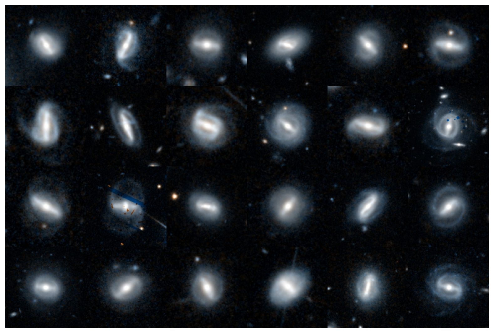
Figure 6: Q1 galaxies predicted as most likely to host strong bars.

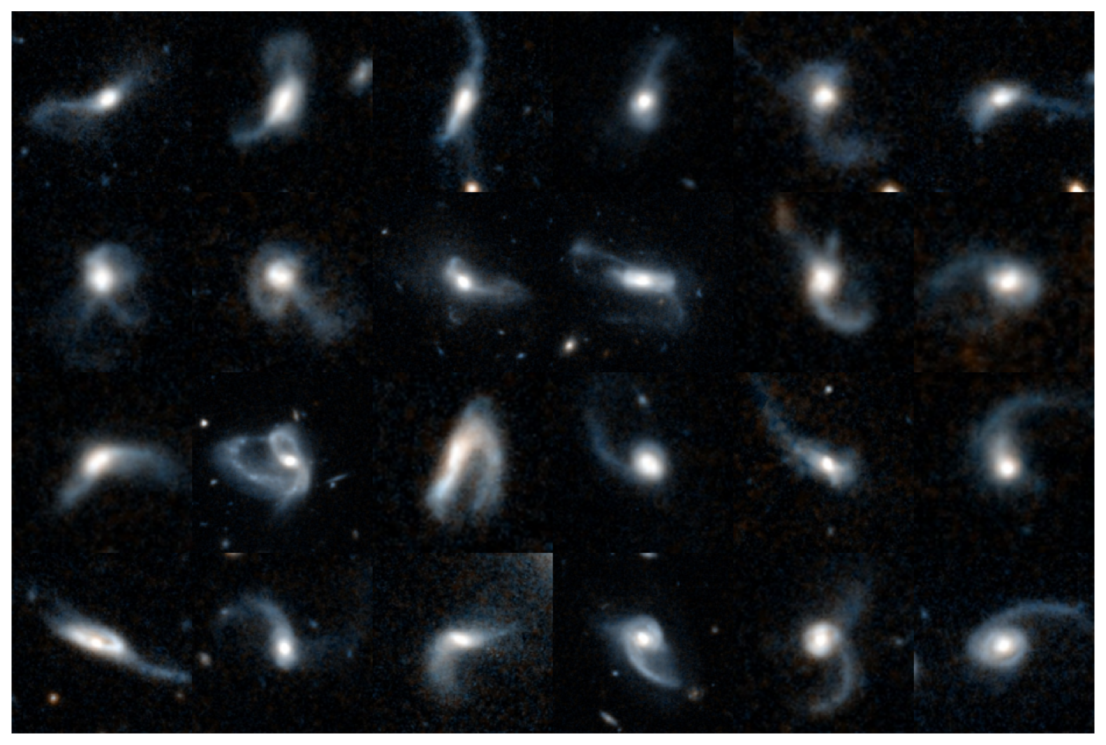
Figure 7: Q1 galaxies predicted as most likely to have a major disturbance (typically interpreted as tidal tails or similar structures, and distinct from ongoing mergers such as close pairs).

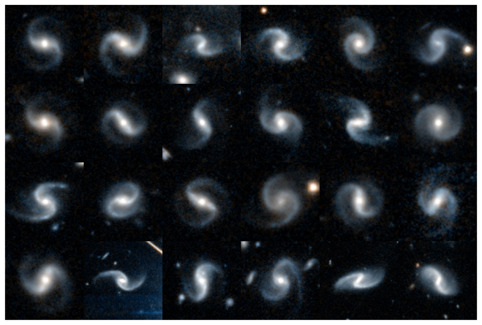
Figure 8: Q1 galaxies predicted as most likely to have exactly two spiral arms.

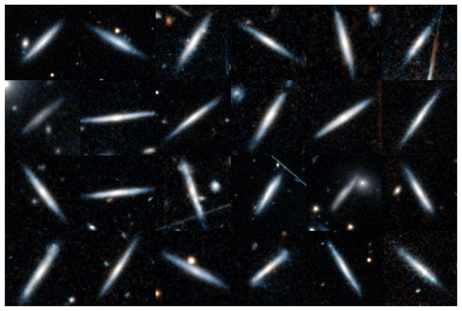
Figure 9: Q1 galaxies predicted as most likely to be bulgeless edge-on disk galaxies. These are likely to be free of recent mergers and hence are useful laboratories for investigating galaxy and supermassive black hole growth (Simmons2013; smethurstEvidenceNonmergerCoevolution2024).

Figure 10: Q1 galaxies predicted as featured but least likely to have spiral arms. Volunteers were never asked to annotate clusters or multi-mergers, but Zoobot has nonetheless learned to extract features that identify such galaxies.

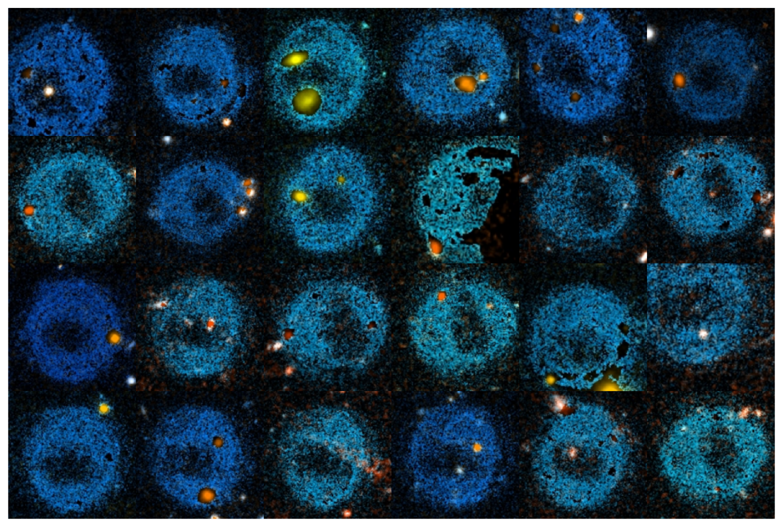
Figure 11: Q1 sources predicted as most likely to be dichrotic ghosts, a well-known artifact caused by internal reflections in telescopes (Euclid Collaboration: Cropper et al. 2024; Euclid Collaboration: Jahnke et al. 2024).

For a quantitative assessment of the performance of our models, we assess their agreement with volunteers on an intensively-annotated subset of intensively-labelled galaxies created for this purpose ($3500$ galaxies each with 25 annotations).

We first report classification metrics. These are created by binning the fraction of volunteers giving each answer (for example, if 60% of volunteers answered ‘Featured’, we bin this label to ‘Featured’). We report metrics on, both all galaxies and (following Domnguez Snchez et al. 2018) on galaxies for whom the class label is confidently known (defined as a volunteer vote fraction above 80% for that answer). Figure 12 shows the resulting confusion matrices.

Our model is near-perfect at all questions when evaluated on high-confidence labels, achieving over 99% accuracy on 7 of 13 questions and no lower than 95% accuracy on any question. Performance including lower-confidence labels is more mixed, which likely reflects firstly, more challenging images for both volunteers and models, and secondly, statistical uncertainty in our binned labels. Figure 13 illustrates this for the first morphology question (‘smooth or featured?’). When the volunteers give a vote fraction decisively skewed to one answer, our model always predicts that answer. As we move to vote fractions near 0.5, the model begins to make nominally incorrect class predictions – but the binomial uncertainty on the volunteer vote fraction suggests that many binned volunteer labels will fall to one side by chance.

We quantify this by simulating the predictions of a perfect model. We do this by, for each galaxy, drawing a new set of 25 trials from a binomial distribution with $p$ set to the actual volunteer vote fraction. Because the outcome of those new trials includes some uncertainty, the fraction of successful trials is not the same as $p$. For example, a true vote fraction just below 0.5 (which we should label as 0) will sometimes give a fraction of successful trials above 0.5 and then be given an incorrect label of 1. In our analogy, these correspond to galaxies where our perfect model has made the correct prediction of $p$, but where the binomial uncertainty in volunteer responses has caused us to record (by misfortune) the wrong label, and so we incorrectly record the model as wrong. When compared to this perfect model, we find that Zoobot is only 30% below the best possible classification accuracy (relative error reduction), primarily attributable to a minor bias towards ‘Featured’.

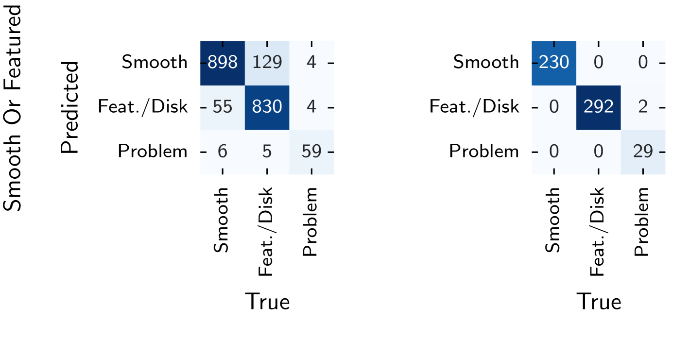
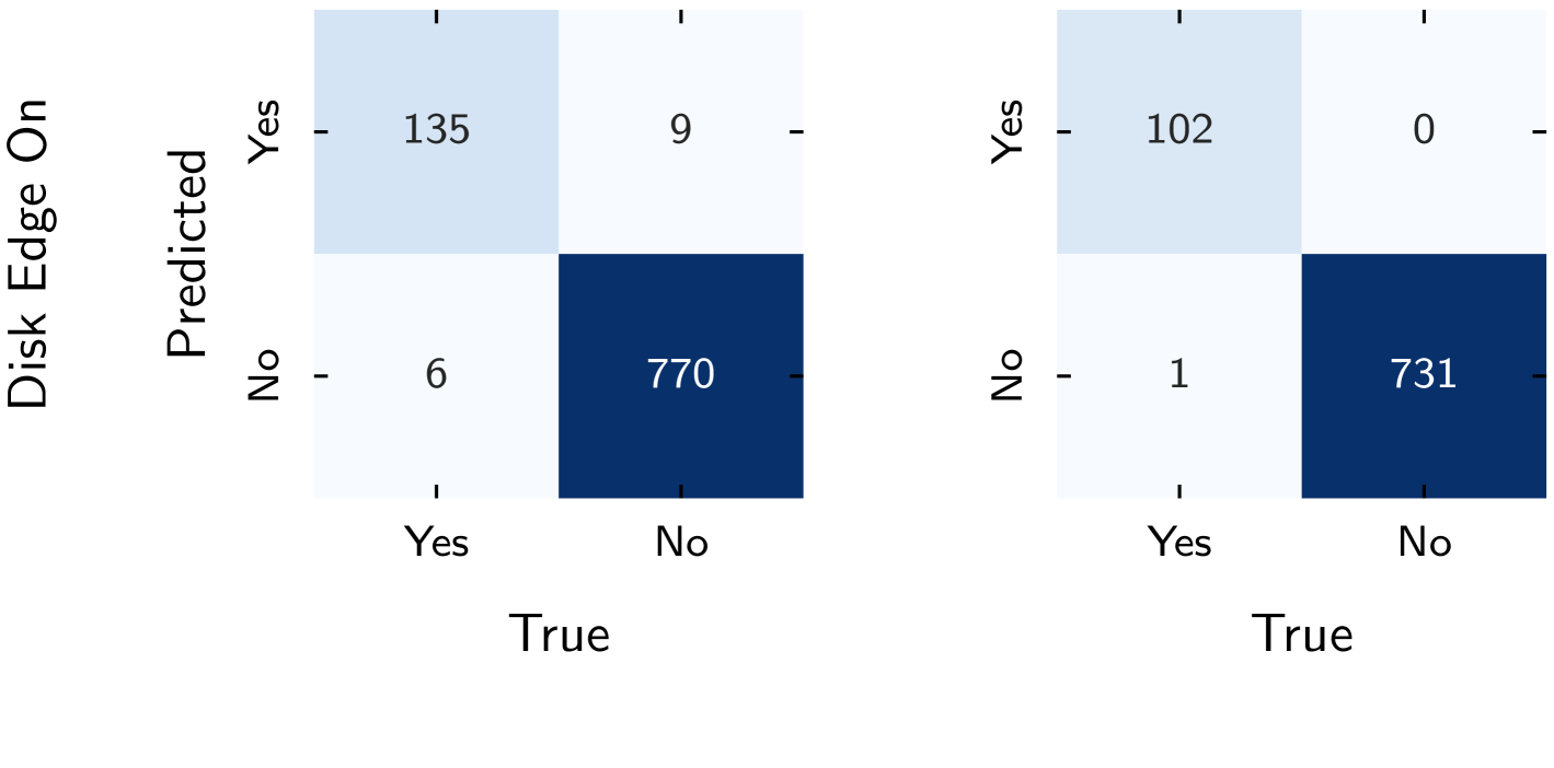
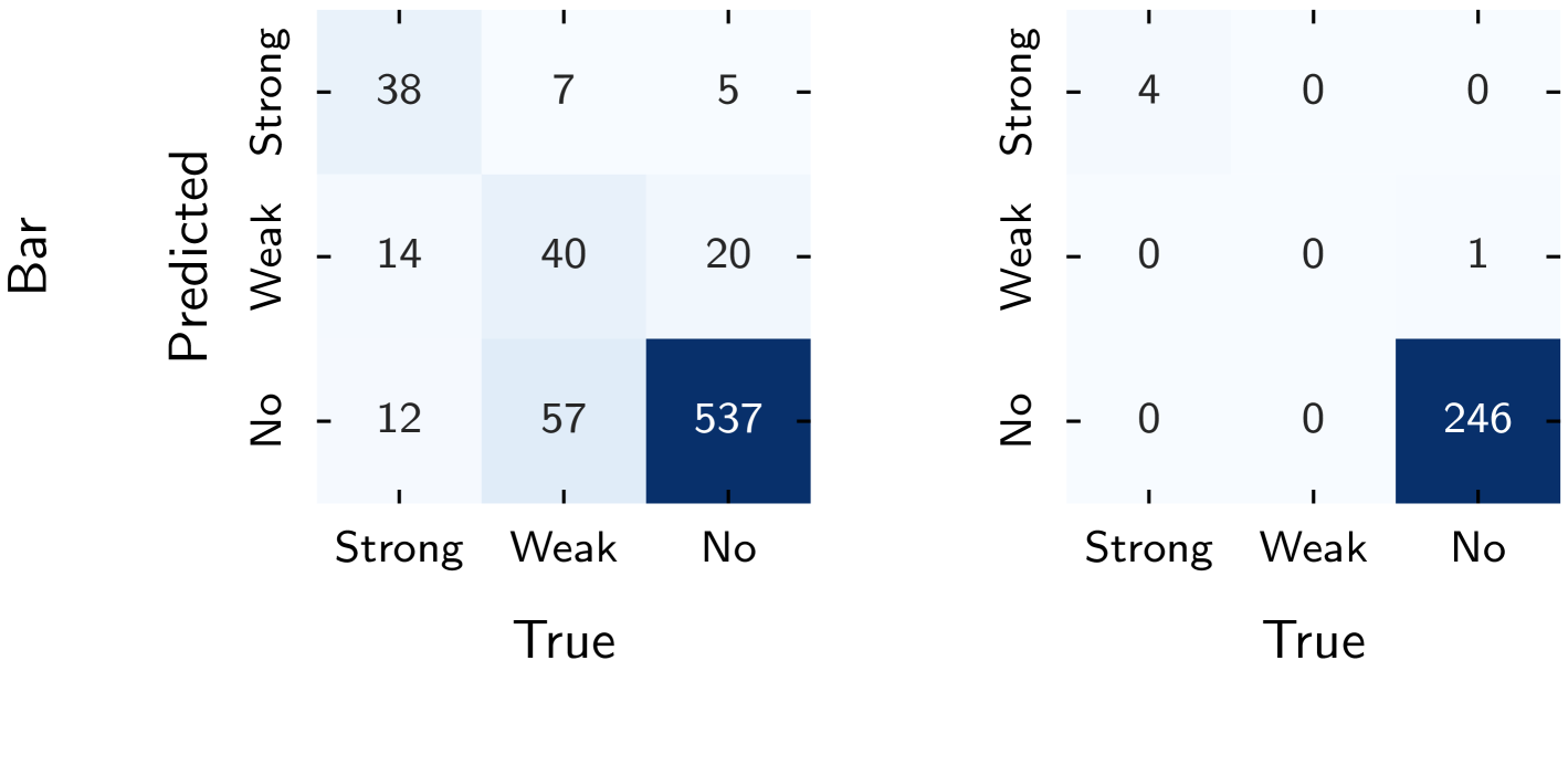
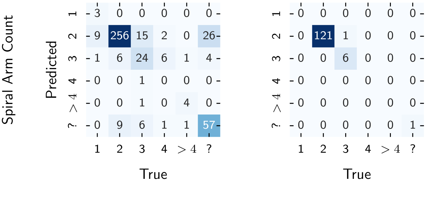
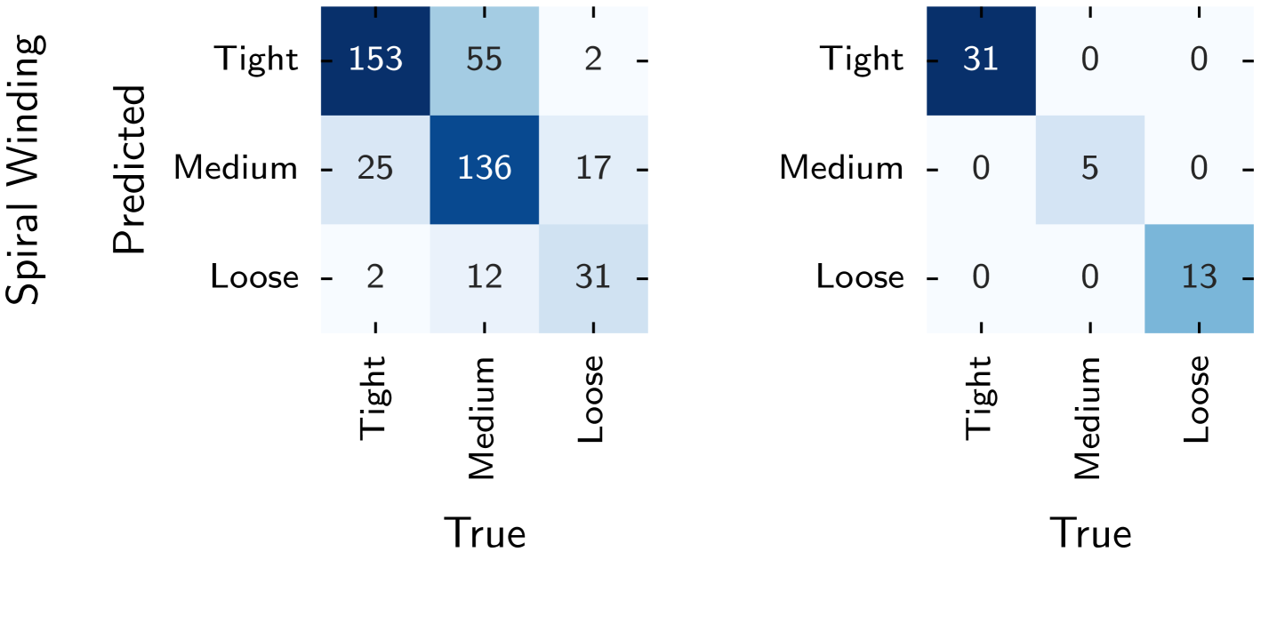
Figure 12: Confusion matrices for the most commonly-used morphology features. Right column includes only galaxies with high confidence (volunteer vote fraction $>0.8$) labels. Our model is near-perfect at all questions when evaluated on high-confidence labels. Performance including lower-confidence labels is more mixed, which likely reflects more challenging images for both volunteers and models.

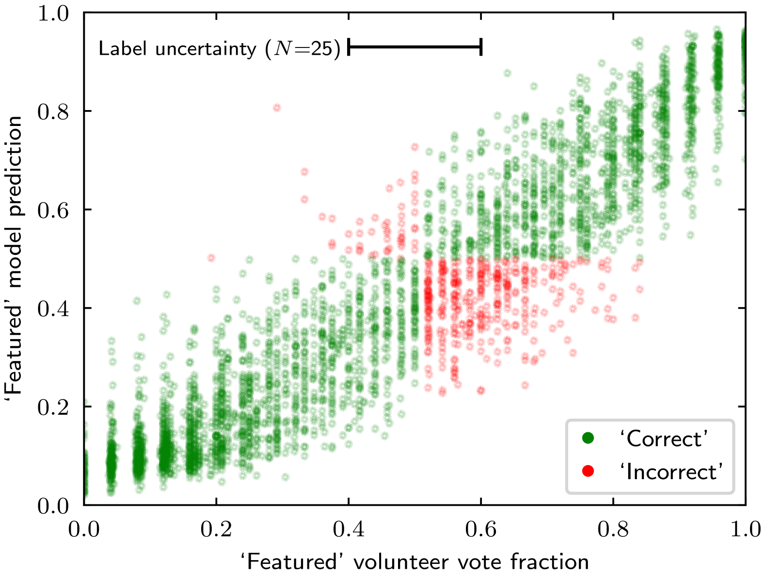
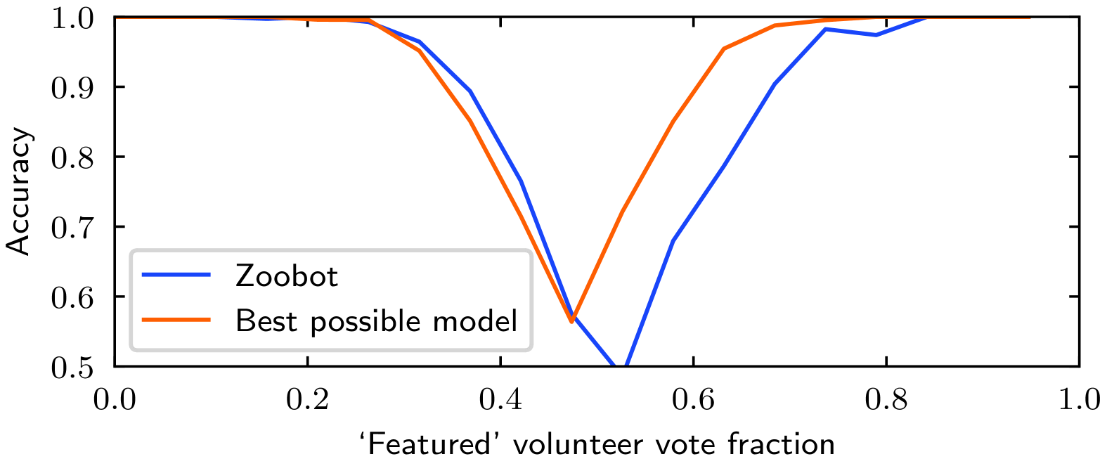
Figure 13: Detailed model performance for the ‘Smooth or Featured?’ question, illustrating the limitations of classification metrics. Above, the measured ($x$-axis) vs. predicted ($y$-axis) ‘Featured’ vote fractions, coloured according to whether the binned prediction equals the binned label (‘correct’) or not (‘incorrect’). Classification errors mostly occur for vote fractions where the true label is uncertain (when the label boundary is within our uncertainty on the vote fraction itself). Below, model accuracy as a function of ‘featured’ vote fraction for either Zoobot or a perfect model (see Sect. 4), illustrating that Zoobot is near-perfect within the uncertainty on our labels.

We next report regression metrics – the ability of our models to predict the fraction of volunteers giving each answer. For example, if 60% of volunteers answering ‘Featured’, our model should predict ‘0.6’. These avoid the noise introduced by either binning uncertain labels or considering only galaxies with confident labels. Figure 14 shows the mean absolute deviation between the predicted and observed volunteer vote fractions (excluding the artifact-related questions, for which we have insufficient examples to calculate reliable metrics). Zoobot typically estimates the volunteer vote fraction to within 10%. Consistent with previous work (walmsleyGalaxyZooDESI2023), increasingly detailed questions are increasingly difficult to precisely predict, with ‘edge-on disk’ predicted most accurately (4% error) and ‘spiral arm count’ least accurately (17% for 2-armed spirals).

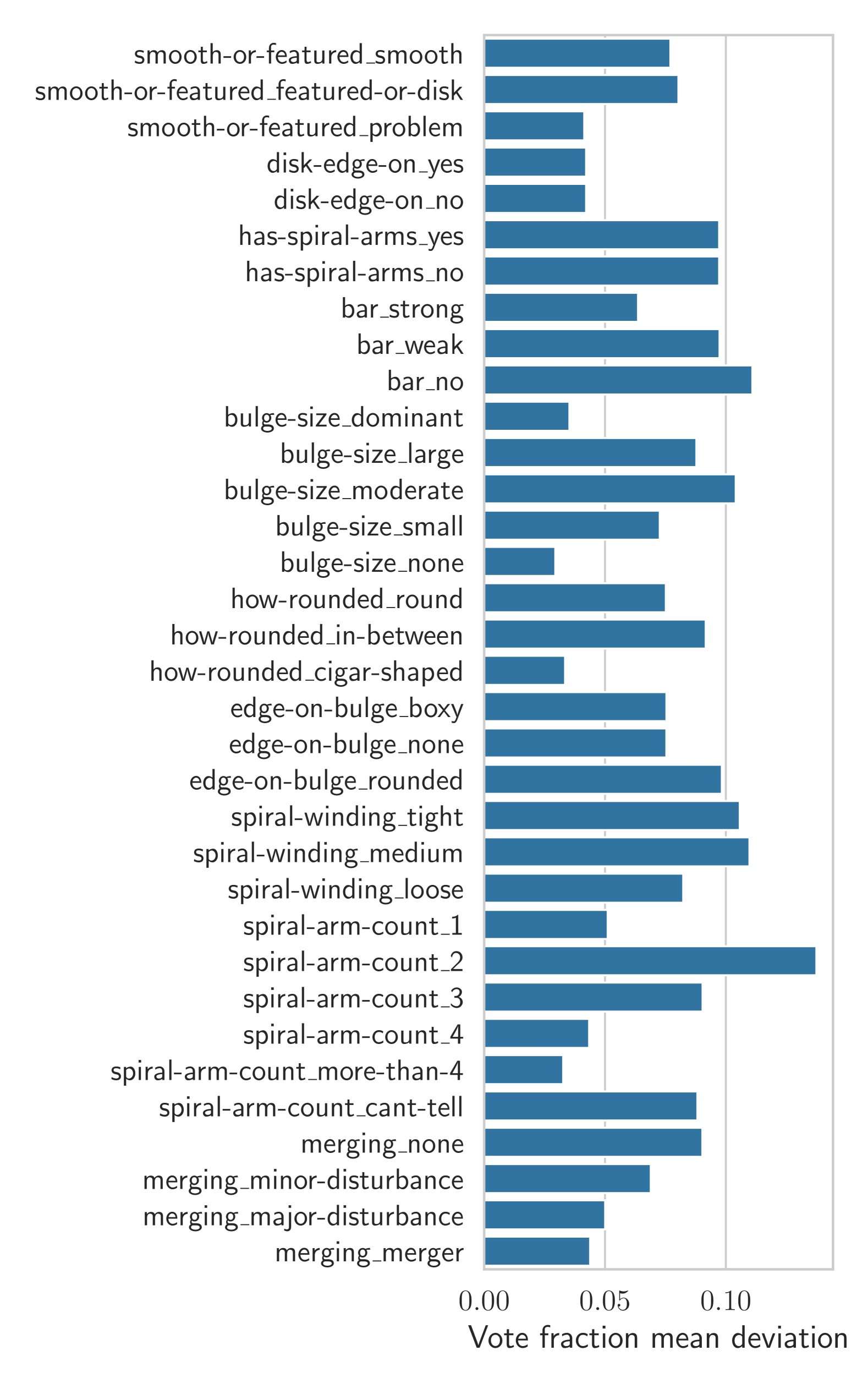
Figure 14: Mean absolute deviation between the predicted and observed volunteer vote fractions. Increasingly detailed questions are increasingly difficult to precisely predict, with the most challenging task being counting spiral arms (17% error for 2-armed spirals). Errors are typically within 10%. For conciseness, ‘clumps’ and ‘problem’ questions are not shown.

5 Data access

All data is available from Zenodo. We also share our data in a machine-learning-friendly format on HuggingFace. This includes the catalogue, the cutout images, the embeddings (vectors summarising the content of each image), and the models. Documentation is provided at those links; below, we provide a summary.

5.1 Catalogues

The dynamic catalogue contains the columns listed below.

• Cross-matching information for the MERge catalogue: object_id ; tile_index.

• id_str. Use to join with embeddings table (below). Formatted like {release_name}_{tile_index}_{object_id}.

• Key MERge catalogue columns for convenience: right_ascension and declination (degrees); kron_radius; mag_segmentation ($I_{\scriptscriptstyle\rm E}$, from flux_segmentation); segmentation_area.

• Paths to jpg cutouts.

• Detailed morphology measurements formatted like

  question_answer_fraction
  (e.g. smooth-or-featured_smooth_fraction),

  question_answer_dirichlet
  (e.g. smooth-or-featured_smooth_dirichlet).

We expect that most catalogue users will be primarily interested in the fraction columns. For example, the column ‘smooth-or-featured_smooth_fraction’ includes the fraction of volunteers predicted by Zoobot to give the answer ‘Smooth’ when asked ‘Is this galaxy smooth or featured?’. They can be combined; for example, ‘smooth-or-featured_featured-or-disk_fraction ¿ 0.5’ and ‘disk-edge-on_no ¿ 0.5’ would select galaxies which are featured and face-on. Catalogue users might use these columns as selection cuts (to investigate galaxies with specific morphologies) or consider how these measurements correlate with other common measurements like mass, star formation rate, location in the cosmic web, etc. There is no ‘best’ choice of cuts, because it depends on your aim; increasing the threshold for any cut will make your sample purer but smaller. We suggest starting generously (with thresholds of 0.5 for most questions, or lower for questions with many or rare answers) and raising your thresholds until the sample reaches your desired purity, as judged from the images.

The pipeline catalogue includes only the Dirichlet values and they are named simply as question_answer. For the Dirichlet columns, each value is a parameter for a Dirichlet distribution. The Dirichlet distribution is the multivariate version of the beta distribution. When both beta parameters (that is, both answers to a morphology question) have low values, the beta distribution is flat, and we are uncertain about the galaxy morphology. When one answer is high, and one answer is low, we are confident in that high answer. The ‘_dirichlet’ columns therefore encode both the predicted vote fraction and the uncertainty on that predicted vote fraction. One can calculate the predicted fraction with $\text{E}(X_{i})=\alpha_{i}/\sum{\alpha}$ and the uncertainty with $\text{Var}(X_{i})=\alpha_{i}(1-\alpha_{i})/(1+\sum{\alpha})$ where $\alpha_{i}$ is the Dirichlet concentration of the chosen answer and $\sum{\alpha}$ is the sum of concentrations for all answers to the chosen question.

The morphology measurements are Zoobot predictions, not volunteer answers. Zoobot predicts every answer to every question. To avoid providing measurements where a question is not relevant (for example, answering how many spiral arms? for a smooth galaxy), we set morphology predictions to NaN where the answer is expected to be not relevant. We define this as a leaf probability (that is, the product of all the vote fractions which led to that question) below 0.5.

The detailed morphology measurements in the pipeline catalogue are released as part of the MER (as in, MERged data, see Euclid Collaboration: Romelli et al. 2025) catalogue. The MER catalogue also includes common measurements like photometry, including photometry from other surveys; please refer to the ESA Euclid Science Archive website for the latest information.

The detailed morphology measurements in the dynamic catalogue are made outside of the official pipeline. This allows more experimentation and flexibility. For example, the dynamic catalogue can use composite $I_{\scriptscriptstyle\rm E}+Y_{\scriptscriptstyle\rm E}$ images, while the official pipeline uses $I_{\scriptscriptstyle\rm E}$ images only. For another example, we can update the model (such as by introducing new labels) and make new predictions at any time. In general, we expect the dynamic catalogue to include the latest ‘bleeding edge’ measurements, while the pipeline catalogue will include slowly-changing measurements that match the release cadence of the Euclid mission data releases. The difference between the dynamic catalogue and pipeline catalogue should reduce over time as we settle into ‘normal operations’.

5.2 Cutouts

We share cutouts of all galaxies in the catalogue, in two formats. For file-based access, we upload our cutouts as part of our Zenodo archive. For machine learning applications, we also share our cutouts on the HuggingFace Hub along with our embeddings (below). Cutouts are saved in native resolution for storage efficiency; you may wish to resize them to a constant size.

Images for all of the galaxies in our catalogue are created from MERge mosaics, described in Euclid Collaboration: Romelli et al. (2025) The original Q1 data is available via the ESA Euclid Science Archive and described in Euclid Collaboration: Aussel et al. (2025).

We also share reference code for creating our images on GitHub. This code is primarily intended for making Euclid cutouts at scale via ESA Datalabs (ESA Datalabs 2021) but also acts as a public record of our exact process.

5.3 Embeddings

We previously (Sect. 3.2) described how foundation models aim to extract image features that summarise the visual content of each image. Each feature is an $N$-dimensional coordinate vector (here, $N=512$) locating (embedding) the image in an N-dimensional space. The linear mapping we describe in Sect. 3.2 aims to learn which volume in this space corresponds to which volunteer answers. But embeddings are also useful for broader tasks such as similarity search, including for galaxy morphology (Stein2021; parker_astroclip_2024; Euclid Collaboration: Siudek et al. 2025).

The Zoobot embeddings are presented on Zenodo and the HuggingFace Hub as a table with rows of galaxies and columns like feat_pca_n, where feat_pca_n is the $N^{\rm th}$ principle component of our higher-dimensional embedding. We include the first 40 components (preserving 94% variance). We also share the uncompressed higher-dimensional embedding, similarly with columns like feat_n. Bear in mind that many methods may struggle (either performing poorly due to the ‘curse of dimensionality’ or becoming impractically slow) in high dimensions.

Figure 15 shows two similarity searches made on the Zoobot Q1 embeddings. Note that these embeddings were not created using any Euclid data (Sect. 3.2).

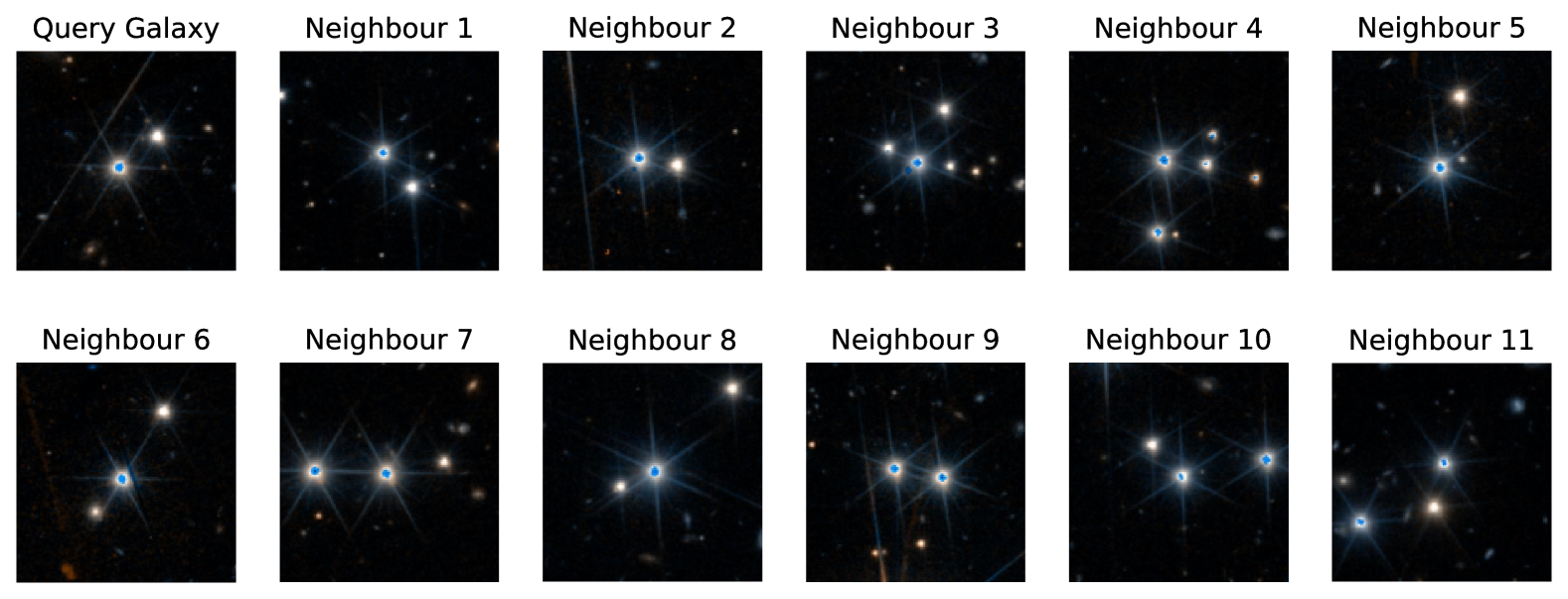
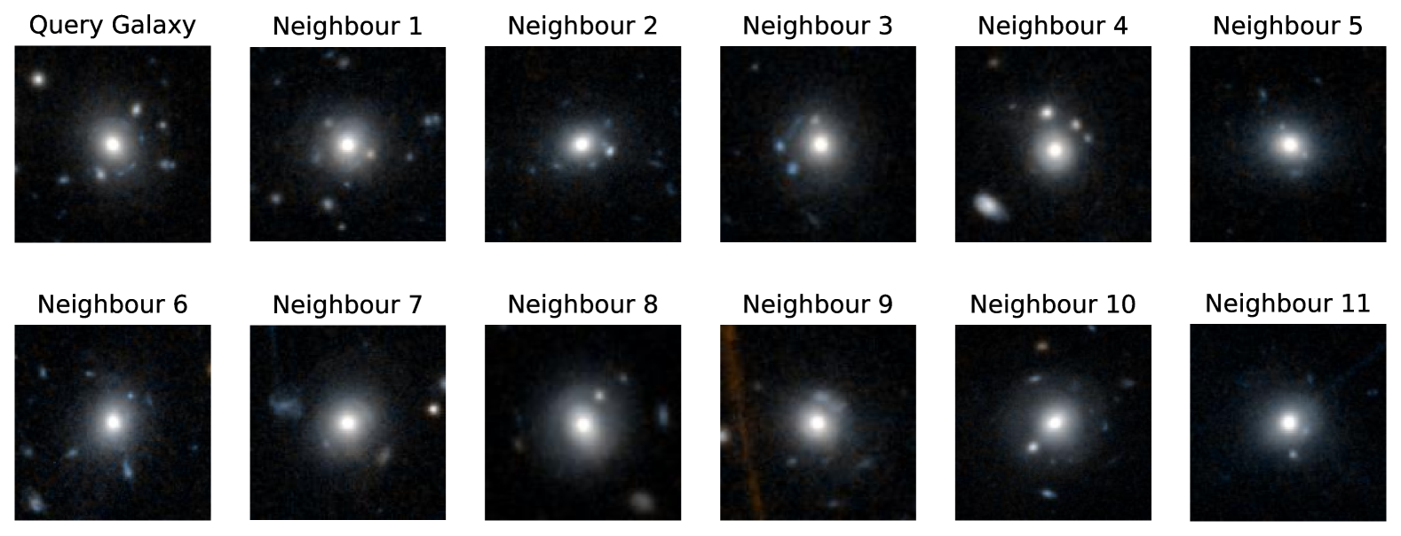
Figure 15: Similarity searches for a pair of stars (above) and strong gravitational lens candidates (below) in Q1.

6 Conclusion and outlook

Our catalogue provides robust visual morphology measurements (e.g., spiral arm counts, bars, mergers) for the bright and extended galaxies in Q1. These measurements complement traditional morphology measurements (Euclid Collaboration: Romelli et al. 2025) and, together, both catalogues provide a comprehensive description of morphology for all Q1 galaxies. Our measurements have already proven useful for addressing a range of science questions; for example, Euclid Collaboration: Huertas-Company et al. (2025) presents new precise measurements of the fraction of barred galaxies out to $z=1$. We look forward to seeing the work of the wider community.

Deep learning does not automatically resolve the fundamental limitations of visual morphology – it only makes them scale. We use human responses to images as our ground truth throughout and do not attempt to correct for observational biases such as redshift or angular size. The catalogue reports what is visible in each image, as a necessary first step to estimating the intrinsic nature of each galaxy. We anticipate that future progress in large-scale galaxy morphology will come not from more accurate models but from models that take a broader interpretation of what learning means (for example, Cranmer 2023 and wuInsightsGalaxyEvolution2024) and from the thoughtful combination of models with other essential astronomy tools like simulations and statistics.

Summarising deep learning for survey astronomy, Huertas-Company & Lanusse (2023) write that ‘the majority of works are still at the proof-of-concept stage’. In this work, we show that one month of volunteer effort is sufficient to make a science-ready morphology catalogue for $10^{8}$ in Euclid, not just as a proof-of-concept but by creating the first rows of that catalogue. The foundation model used was only trained on Euclid data for a final linear mapping. We used it to create a galaxy morphology catalogue; we might have chosen another image task. A similar approach has proven successful on strong lenses (Euclid Collaboration: Walmsley et al. 2025), active galactic nuclei (Euclid Collaboration: Margalef-Bentabol et al. 2025), star-forming clumps (poppTransferLearningGalaxy2024), mergers (Margalef-Bentabol et al. 2024), tidal features (Omori et al. (2023); ), anomaly searches (Lochner & Rudnick 2024), segmentation sazonova_structural_2022, etc. We encourage the reader to experiment with using the tools behind our catalogue – the foundation models, and the code to adapt them – to create exactly the catalogue needed for each science case.