Euclid Quick Data Release (Q1)

We present the results of the single-component Sérsic profile fitting for the magnitude-limited sample of $I_{\scriptscriptstyle\rm E}$ $<23$ galaxies within the 63.1 deg² area of the Euclid Quick Data Release (Q1). The associated morphological catalogue includes two sets of structural parameters fitted using SourceXtractor++: one for VIS $I_{\scriptscriptstyle\rm E}$ images and one for a combination of three NISP images in $Y_{\scriptscriptstyle\rm E}$, $J_{\scriptscriptstyle\rm E}$ and $H_{\scriptscriptstyle\rm E}$ bands. We compare the resulting Sérsic parameters to other morphological measurements provided in the Q1 data release, and to the equivalent parameters based on higher-resolution Hubble Space Telescope imaging. These comparisons confirm the consistency and the reliability of the fits to Q1 data. Our analysis of colour gradients shows that NISP profiles have systematically smaller effective radii ($R_{\rm e}$) and larger Sérsic indices ($n$) than in VIS. In addition, we highlight trends in NISP-to-VIS parameter ratios with both magnitude and $n_{\rm VIS}$. From the 2D bimodality of the $(u-r)$ colour-$\log(n)$ plane, we define a $(u-r)_{\rm lim}(n)$ that separates early- and late-type galaxies (ETGs and LTGs). We use the two subpopulations to examine the variations of $n$ across well-known scaling relations at $z<1$. ETGs display a steeper size–stellar mass relation than LTGs, indicating a difference in the main drivers of their mass assembly. Similarly, LTGs and ETGs occupy different parts of the stellar mass –  star-formation rate plane, with ETGs at higher masses than LTGs, and further down below the Main Sequence of star-forming galaxies. This clear separation highlights the link known between the shutdown of star formation and morphological transformations in the Euclid imaging data set. In conclusion, our analysis demonstrates both the robustness of the Sérsic fits available in the Q1 morphological catalogue and the wealth of information they provide for studies of galaxy evolution with Euclid.

1 Introduction

The study of galaxy morphology is a topic as old as galaxy science itself, which started with the Hubble sequence (Hubble 1926), where galaxies were classified according to their shapes and features. This sequence challenges any theory of galaxy formation and evolution to explain how such diversity arose across the history of the Universe.

Morphology has remained a topical issue for all galaxy scientists due to its many connections to other aspects of galaxy formation. On one hand, the galaxy-morphology density relation (Dressler 1980) first quantified that different morphological types of galaxies are located in different environments with respect to large-scale structures. On the other hand, the colour bimodality of galaxy populations is related to the morphology, since red and blue galaxies are predominantly early- and late-type galaxies (Strateva et al. 2001; Baldry et al. 2004; Allen et al. 2006). The correlation between the morphology and star-forming state of galaxies was further investigated to understand the causal relation linking morphological transformations from late- to early-type galaxies and the shutdown of star formation, known as the quenching of galaxies (Schawinski et al. 2014; Bremer et al. 2018; Quilley & de Lapparent 2022; de Sá-Freitas et al. 2022; Dimauro et al. 2022). Notably, the growth of the bulges of galaxies has been shown to correlate with the quenching of galaxies in observational studies (Lang et al. 2014; Bluck et al. 2014; Bremer et al. 2018; Bluck et al. 2022; Dimauro et al. 2022; Quilley & de Lapparent 2022). In that regard, Martig et al. (2009) proposed a morphological quenching process in which the bulge of a galaxy, when it becomes massive enough, can stabilise the disc against cloud fragmentation, preventing further star formation. But other phenomena could also explain these trends, with black hole growth (Bluck et al. 2022; Brownson et al. 2022) correlated with bulge growth, and eventually leading to quenching by active galactic nucleus (AGN) feedback (Silk & Rees 1998; Croton et al. 2006; Chen et al. 2020).

There are several ways to characterise galaxy morphologies. The earliest analyses relied on visual classification (Hubble 1926; Nair & Abraham 2010; Baillard et al. 2011), however that was a time-consuming and human-based task. Automatic and quantitative methods were thus later developed. Notably, parametric surface-brightness fitting, based on the Sérsic function (Sérsic 1963), became a widely used method to characterise galaxy morphology and obtain estimates of their sizes and shapes (Trujillo et al. 2004; Kelvin et al. 2012; Morishita et al. 2014; Mowla et al. 2019; Kartaltepe et al. 2023; Lee et al. 2024, among many others). For spiral and lenticular galaxies, the use of two distinct profiles, usually a Sérsic profile to model the bulge, and an exponential one (Sérsic profile with a fixed Sérsic index $n$ of 1) for the disc, have led to improvements in fitting the full surface brightness profiles of galaxies, and most importantly provides more physically meaningful parameters (Meert et al. 2015; Lange et al. 2016; Margalef-Bentabol et al. 2016; Dimauro et al. 2018; Fischer et al. 2019; Casura et al. 2022; Hashemizadeh et al. 2022; Quilley & de Lapparent 2022).

The Euclid space mission (Euclid Collaboration: Mellier et al. 2024) is envisioned to observe an effective sky area of roughly 14 000 ${\rm deg^{2}}$ in order to map the evolution of the large-scale structure, and will therefore observe a number of resolved galaxies several orders of magnitude larger than other previous missions such as the Hubble Space Telescope or the James Webb Space Telescope. It will cover from the red optical region using the Visible Imager (VIS; with a single broadband filter $I_{\scriptscriptstyle\rm E}$, Euclid Collaboration: Cropper et al. 2024; Euclid Collaboration: McCracken et al. 2025) to the near infra-red (NIR) using the Near-Infrared Spectrometer and Photometer (NISP). The latter enables both imaging in the NIR through three filters $Y_{\scriptscriptstyle\rm E}$, $J_{\scriptscriptstyle\rm E}$, $H_{\scriptscriptstyle\rm E}$ and low-resolution NIR spectroscopy (Euclid Collaboration: Jahnke et al. 2024; Euclid Collaboration: Schirmer et al. 2022; Euclid Collaboration: Polenta et al. 2025). Therefore, the large sky area of the Euclid mission, combined with the exquisite spatial resolution of its instruments (pixel sizes of $0.\mathrm{″}1$ and $0.\mathrm{″}3$ and a point spread function (PSF) full width at half maximum (FWHM) of $0.\mathrm{″}16$ and $0.\mathrm{″}48$ for the optical and NIR, respectively), and the unparalleled surface brightness sensitivities expected to be reached (approximately 29.8 mag arcsec^-2 for the Euclid Wide, EWS; Euclid Collaboration: Scaramella et al. 2022, and 31.8 mag arcsec^-2 for the Euclid Deep, EDS), make it uniquely suited for groundbreaking discoveries.

Preliminary work has already been conducted to evaluate how beneficial Euclid will be to perform morphological analyses combining statistics, precision, and redshift coverage. Using deep generative models, Euclid Collaboration: Bretonnière et al. (2022) estimated that the EWS and EDS would be able to resolve the inner structure of galaxies down to surface brightness of 22.5 mag arcsec² and 24.9  mag arcsec², respectively. Furthermore, the Euclid Morphology Challenge (EMC) compared and estimated the performance of five luminosity-fitting codes in retrieving the photometry (Euclid Collaboration: Merlin et al. 2023) and structural parameters (Euclid Collaboration: Bretonnière et al. 2023). It concluded that single-Sérsic fits and bulge and disc decomposition were reliable up to an $I_{\scriptscriptstyle\rm E}$ of 23 and 21, respectively. The SourceXtractor++ software (Bertin et al. 2020; Kümmel et al. 2022) showed a high level of performance and was therefore chosen to perform the fits included in the Euclid data processing function.

Moreover, a first morphological analysis based on Euclid data using luminosity profile-fitting was performed in Quilley et al. (2025, Q25a hereafter), where galaxies in the Early Release Observations (ERO) of the Perseus cluster (Cuillandre et al. 2024) were modelled, focusing not on the cluster itself but on the thousands of background galaxies present. This study represents the first demonstration of how the quality of Euclid images can enable morphological analyses and notably measured a bulge-disc colour dichotomy, as well as colour gradients within discs for galaxies up to $z<0.6$ (Q25a).

In this work, we first present the catalogue obtained by performing Sérsic fits on all the galaxies detected in the first Euclid Quick Data Release (Q1), and then leverage them to reassert the importance of morphological transformations in galaxy evolution. These new Q1 data are described in Sect. 2, together with the galaxy sample that will be used throughout this analysis. In Sect. 3, we detail the choices made in the configuration of the Sérsic fits. In Sect. 4, we present the distributions of the best-fit Sérsic parameters. In Sect. 5, we compare the Sérsic parameters to other morphological indicators available in the Q1 data, or from previous HST studies, to discuss their consistencies. In Sect. 6, we investigate the variations of the Sérsic parameters with observing band, by comparing the values derived from the VIS image to those obtained on the three NISP images, which allow us to probe galaxy colour gradients. In Sect. 7, we emphasise the role of morphology in galaxy evolution, first by establishing the bimodality of galaxy populations in terms of colour, mass and morphology, and then by examining the variation of the Sérsic index across key scaling relations such as the size–stellar mass and the star-formation rate (SFR)–stellar mass relations.

2 Data

This work focuses on data from Euclid Quick Release Q1 (2025, Q1), which covered over 63.1 deg² of the sky during three sessions in 2024. They targeted the different Euclid Deep Fields (EDFs): EDF-North,  22.9 deg², EDF-Fornax,  12.1 deg²), and EDF-South,  28.1 deg². The Q1 data are representative of standard EWS observations conducted as a single Reference Observation Sequence. For additional details on the Q1 data and its processing, we refer the reader to Euclid Collaboration: Aussel et al. (2025).

The analysis presented in this work focuses on the Q1 tiles from the EDFs. Each tile has a field of view of 0.57 deg² ($0.\mathrm{°}75$$\,\times$ $0.\mathrm{°}75$). Observations followed a dithered sequence: simultaneous imaging in the $I_{\scriptscriptstyle\rm E}$ filter and NIR slit-less grism spectra, followed by NIR imaging through the $Y_{\scriptscriptstyle\rm E}$, $H_{\scriptscriptstyle\rm E}$, and $J_{\scriptscriptstyle\rm E}$ filters. The telescope was dithered between observations, and the sequence was repeated four times. Exposure times were 1864 s for the $I_{\scriptscriptstyle\rm E}$ filter and 348.8 s for each NIR filter, and photometric calibration uncertainty was constrained to less than 10$\%$, with zero points of $I_{\rm AB}$=23.9 for all bands. AB magnitudes are referred to simply as magnitudes throughout this work.

To construct the final sample of galaxies from the Q1 data set, we used photometric data extracted from the photometric catalogues produced by the OU-MER pipeline (Euclid Collaboration: Romelli et al. 2025). In addition to Euclid data, it also includes external data from ground based-surveys, that provides optical photometry in bands narrower than $I_{\scriptscriptstyle\rm E}$, that are useful for photometric redshift computation and spectral energy distribution (SED)-fitting (Euclid Collaboration: Tucci et al. 2025). More specifically, $griz$ photometry from DES (Abbott et al. 2021) is used in EDF-S and EDF-F, whereas for the EDF-N, $ugriz$ photometry is provided by CFIS ($u$ and $r$, Ibata et al. 2017), Pan-STARRS ($i$, Magnier et al. 2020) and HSC ($g$ and $z$, Aihara et al. 2018). A series of selection criteria were then applied to ensure the robustness and reliability of the analysis, as outlined below:

• VIS$\_$DET = 1 to ensure that galaxies are detected in the VIS filter;

• spurious$\_$flags = 0 to prevent spurious sources from contaminating our sample;

• point$\_$like$\_$prob $\leq$ 0.1 to discard point-like sources;

• $I_{\scriptscriptstyle\rm E}$ $\leq$ 24.5, for the largest sample available, but we mostly restrain it to $I_{\scriptscriptstyle\rm E}$ $<23$ for reliability purposes, and when not specified otherwise.

By applying these selection criteria, we obtained a sample consisting of 1 312 068 galaxies up to $I_{\scriptscriptstyle\rm E}$ $<23$ that will be used throughout Sects. 4 and 5. In Sects. 6 and 7, where galaxies will be investigated as a function of redshift, we will use the median of the redshift posterior distribution derived through the spectral energy distribution fitting (see Euclid Collaboration: Tucci et al. 2025). Therefore, we further added the following selection criteria to ensure the reliability of the photometric redshift, as well as of the physical parameters derived:

• the offset between the median redshift derived by SED-fitting to determine the physical properties of galaxies PHZ$\_$PP$\_$MEDIAN$\_$Z and the photometric redshift PHZ$\_$MEDIAN derived for cosmology is less than 0.2;

• the offset between the median PHZ$\_$PP$\_$MEDIAN$\_$Z and the mode PHZ$\_$PP$\_$MODE$\_$Z of the redshift posterior distribution is less than 0.2;

• phys$\_$param$\_$flags = 0.

With these additional selection criteria, we obtained a final sample of 774 837 galaxies with redshifts up to 1.3.

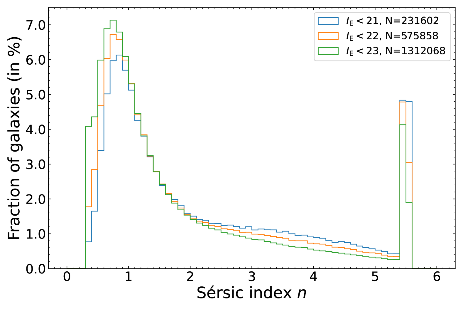
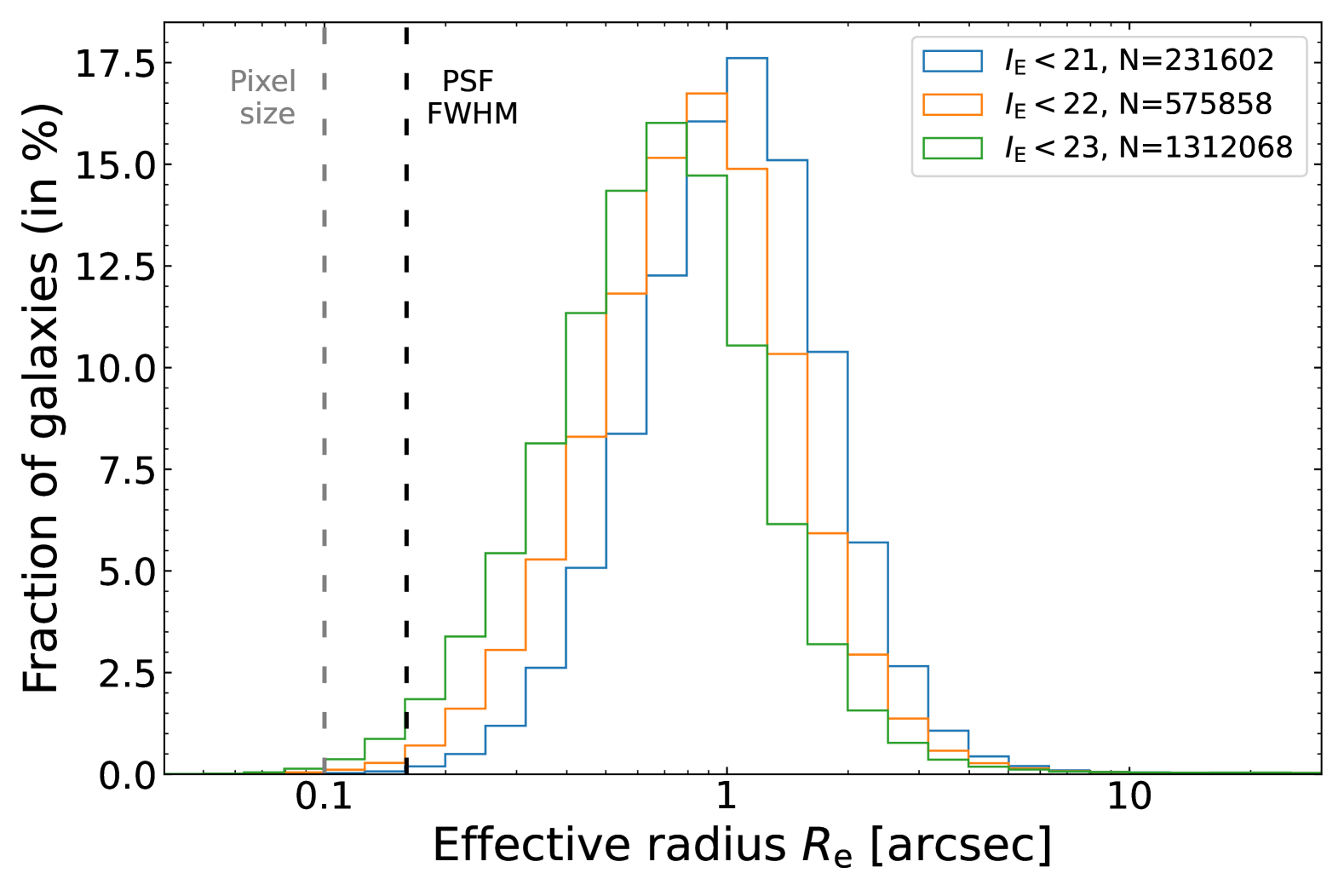
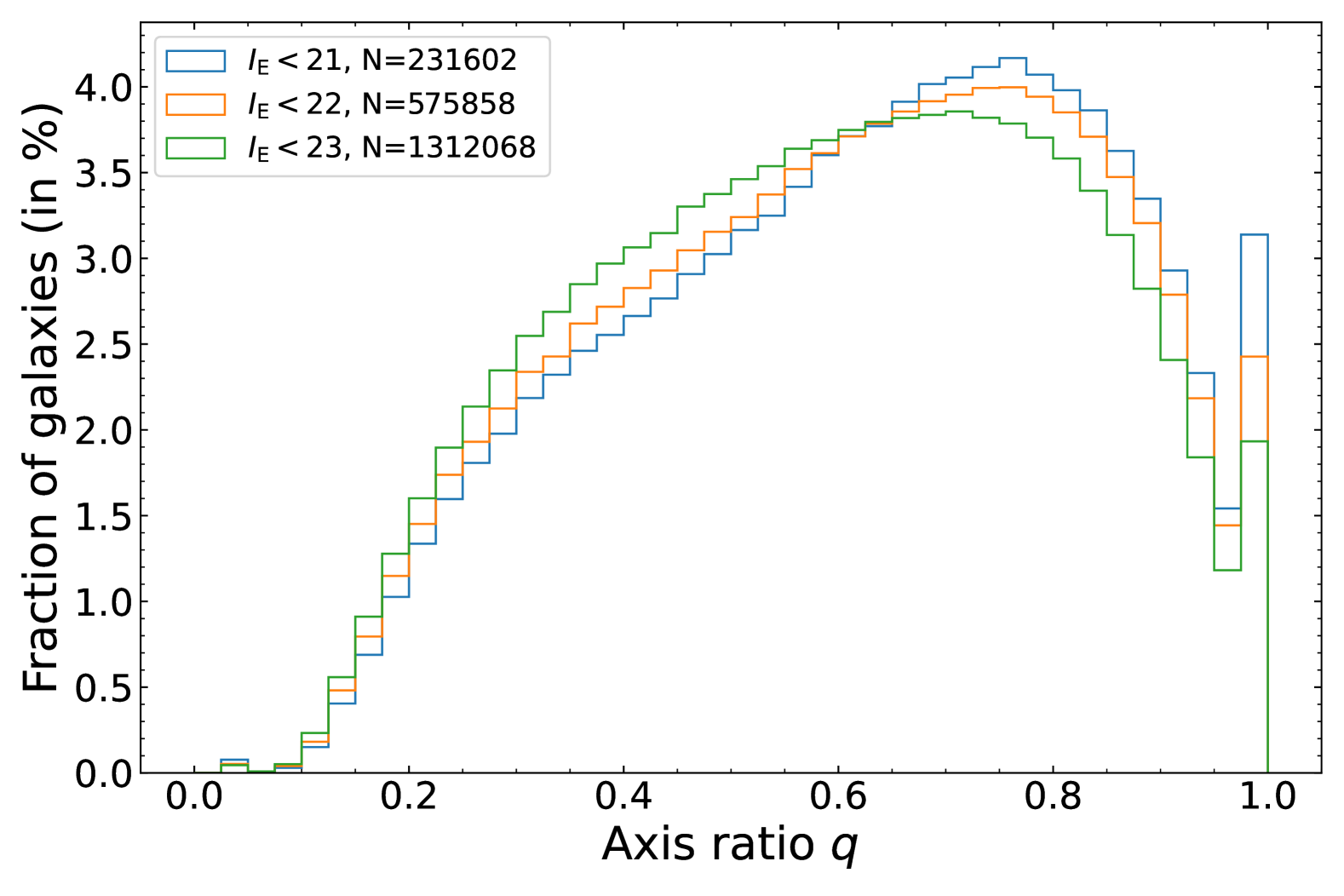
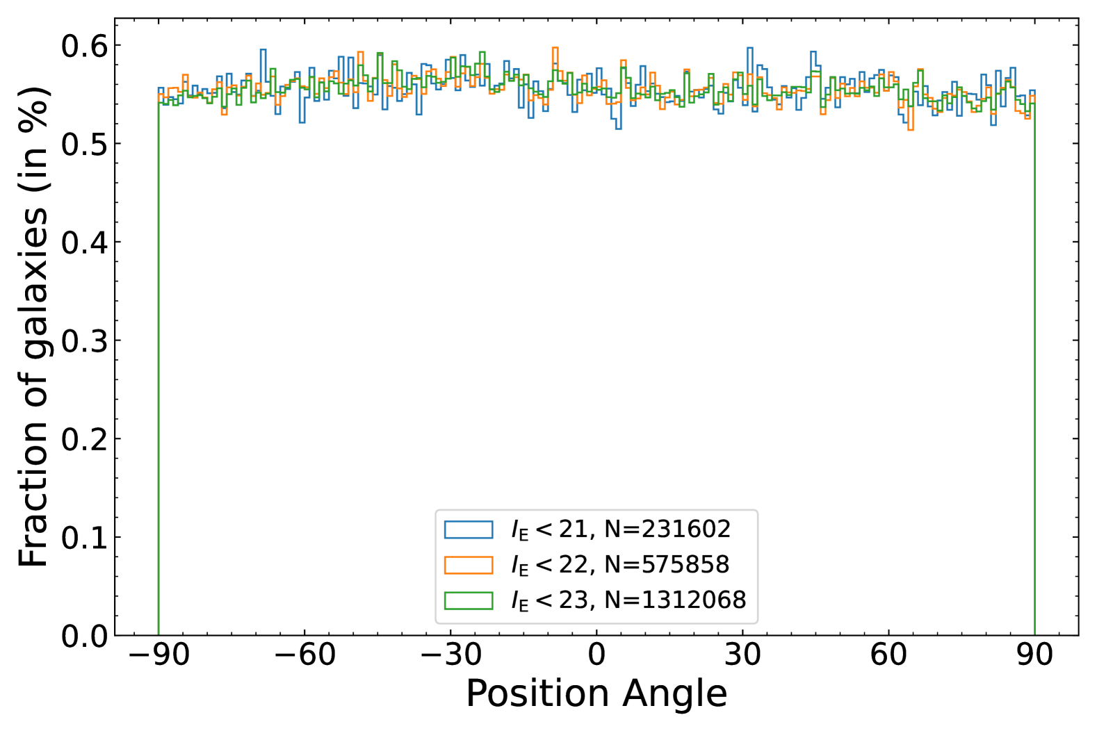
Figure 1: Fractional distributions of parameters of the fitted Sérsic profiles (from left to right and from top to bottom): Sérsic index ($n$), effective radius ($R_{\rm e}$), axis ratio ($q$), and position angle. The blue, orange and green curves correspond to samples down to a limiting $I_{\scriptscriptstyle\rm E}$ of 21, 22, and 23, respectively. The number of galaxies in each sample is indicated in each insert. The $n$ values peak around 0.8, and then sharply decrease until $n\sim 2$, there is a tail of higher values, and an “artificial” peak at the limit of the parameter space at $n=5.5$ (see text). The distributions of $R_{\rm e}$ peak around $1.\mathrm{″}0$, with lower values for fainter magnitudes. The pixel sizes and PSF FWHM are indicated as vertical dotted lines.

3 Methodology

The software SourceXtractor++, whose level of performance was assessed in the EMC, is used to fit elliptically symmetric two-dimensional Sérsic profiles (Sérsic 1963) to all galaxies detected in Euclid images. We recall here the one-dimensional Sérsic function, which describes the variation of the light intensity $I$ as a function of the angular radius $r$:

$$I(r)=I_{\mathrm{e}}\exp\left\{-b_{n}\left[\left(\frac{r}{R_{\mathrm{e}}}\right)^{1/n}-1\right]\right\}\,,$$ (1)

with $R_{\mathrm{e}}$ the major-axis of the elliptical profile that encloses half of the total light (or effective radius), $I_{\mathrm{e}}=I(R_{\mathrm{e}})$ the light intensity at $R_{\mathrm{e}}$, $n$ the Sérsic index characterizing the steepness of the profile, and $b_{n}$ a normalisation parameter depending solely on $n$. Because we are fitting 2D elliptical profiles, the parameters fully describing the profile also include a position angle and an axis ratio, $q$.

The Sérsic fitting procedure uses two sets of structural parameters ($R_{\mathrm{e}}$, $n$, and $q$), one for the VIS image alone, and another one common for the three NISP images. The fits were performed with a common position angle for the two models. This model fitting on the Euclid images provides the aforementioned parameters as well as model photometry in the $I_{\scriptscriptstyle\rm E}$, $Y_{\scriptscriptstyle\rm E}$, $J_{\scriptscriptstyle\rm E}$, and $H_{\scriptscriptstyle\rm E}$ bands. Then, for the external data images, the structural parameters of the Sérsic profiles obtained from the VIS image are used and only magnitudes are allowed to vary to obtain model photometry from these optical bands. This configuration was decided in order to fully benefit from the enhanced spatial resolution of VIS while obtaining colour information, through the comparison of VIS and near-IR parameters (see Sect. 6).

The exact ranges and initial values for all parameters are given below:

• $R_{\mathrm{e}}$ is initialised at the isophotal semi-major axis $a$ (see Sect. 5.1 for details), and spans exponentially the [0.01 $a$, 30 $a$] interval

• $n$ is initialised at 1 and spans linearly the [0.3, 5.5] range

• $q$ is initialised at the isophotal axis ratio and spans exponentially the [0.03, 1] interval

• $q$ is initialised at the isophotal position angle without any bounds, and is reprojected onto the $[-$$,\,$$]$ range

• the $x$ and $y$ coordinates of the centre of the profile are fixed using the built-in function o.centroid from SourceXtractor++

For reproducibility purposes, the configuration files used within the Euclid pipeline, as well as an example image are available at https://cloud.physik.lmu.de/index.php/s/3K4KemBsw5y9yqd, with appropriate documentation. This allows anyone to run SourceXtractor++ single-Sérsic fits on Euclid images in the configuration described throughout this section.

4 Distributions of the structural parameters

We present in Fig. 1, the fractional distributions of $n$, $R_{\rm e}$, $q$, and position angles of the Sérsic profiles fitted on the VIS images out to $I_{\scriptscriptstyle\rm E}$ of 21, 22, and 23 (the total number of objects are indicated in the inserts). The distributions of $n$ peak around 0.75–0.80 and decrease up to the maximum value of 5.5, at which a second peak is observed. The latter corresponds to fits reaching the limit of the parameter space (see Sect. 3). Therefore, fits with $n>5.45$ should be flagged and removed from any Sérsic-based analysis. $R_{\rm e}$ show distributions peaking around $1.\mathrm{″}0$, with lower peaks, and overall histograms shifting towards smaller $R_{\rm e}$ for fainter magnitudes. 94.1% of the sources with $I_{\scriptscriptstyle\rm E}$ $<23$ have an effective diameter larger than 3 times the PSF FWHM. The axis ratios show broad distributions with peaks around 0.71, 0.75, and 0.76 at the three magnitude limits, framed by a sharp peak at $q=1.00$ and a small bump around $q=0.03$ corresponding to the bounds of the parameter space. Visual inspection of the fits with $q<0.05$ shows that these sources correspond to stars not correctly masked, diffraction spikes, or cosmic rays, so they should be flagged and removed from the analysis. However, the situation for $q=1.00$ is different because those objects are galaxies that visually appear rather round and sometimes with slight asymmetries. However, the best-fit solution returned is not necessarily the absolute best-fit possible and instead corresponds to a local minimum in the parameter space due to the limit at $q=1.00$. All the outliers identified in this section are removed in the rest of the analysis.

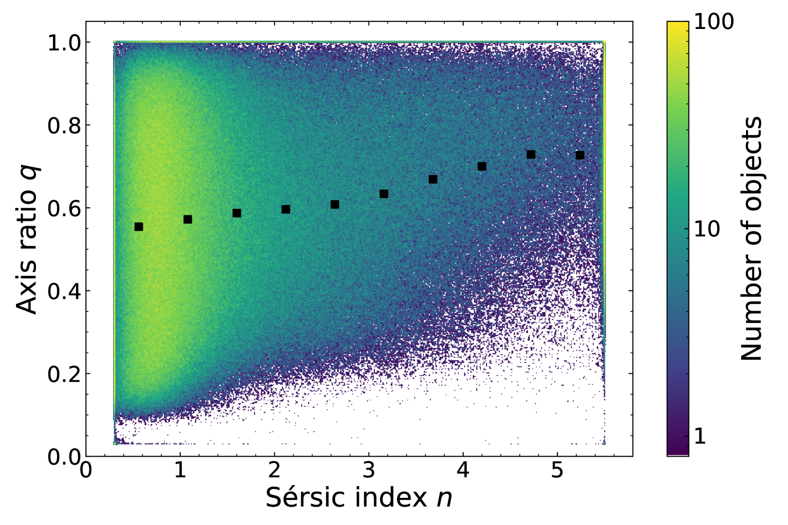
Figure 2: Axis ratio $q$ versus Sérsic index $n$ of the fitted profiles. Black squares indicate the running median $q$ in bins of $n$. Pure discs ($n\sim 1$) can be seen at all inclinations, from edge-on to face-on, leading to a wide range of $q\in[0.1,\,1.0]$, with a lower density of object for the most extreme cases at its edges. For higher values of $n$, either the bulge “bulging out” from the disc or more spheroidal galaxies prevent very low $q$.

The $q$ measured in projection onto the sky depend on the tri-dimensional shape of the galaxies, characterised by their axes $a$, $b$, and $c$, as well as the orientation at which we observe them (see e.g. van der Wel et al. 2014a; Pandya et al. 2024. disc galaxies can be observed at all inclinations, from face-on to edge-on. They thus can display $q$ going from the physical one of the disc, $b/a$, close to 0.8–0.9 (since discs are almost but not perfectly circular; Padilla & Strauss 2008; Rodr´ıguez & Padilla 2013), to the ratio between their disc thickness and radius (taking values between $c/a$ and $c/b$; Favaro et al. 2024). Figure 2 shows the distribution of $q$ versus $n$ and confirms that for pure disc morphologies ($n\lesssim 1$), all $q$ within [0.1, 1] are found. For higher $n$ the lower bound of the envelope of points increases to higher $q$. This is first due to the emergence of bulges in spiral galaxies ($n\sim 2-3$), which are also included in the Sérsic fit and bias the profile towards larger $q$ than those for the discs, as shown by Q25a. This trend continues for $n\gtrsim 4$, corresponding to early-type morphologies, especially elliptical galaxies, which are predominantly oblate spheroids, and thus their values of $c/a$ are higher than for discs (Padilla & Strauss 2008; Rodr´ıguez & Padilla 2013).

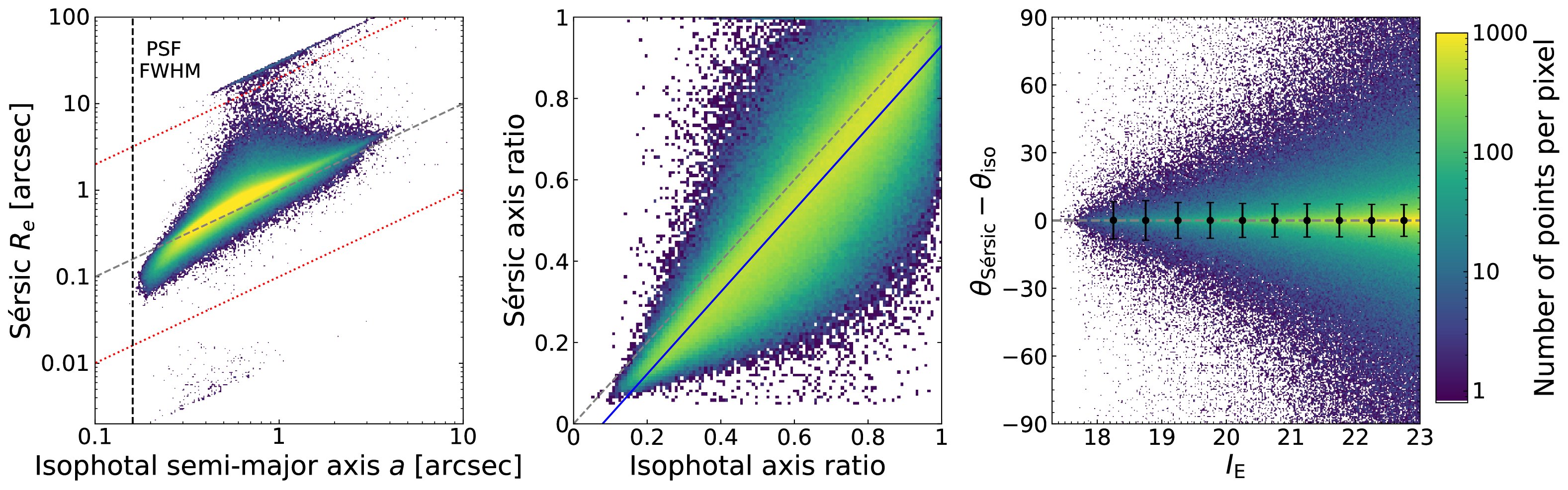
Figure 3: Comparison between structural parameters of the Sérsic profiles and isophotal measures for $I_{\scriptscriptstyle\rm E}$ $\leq 23$, with a colour-map indicating the density of points. Left: Sérsic effective radius $R_{\rm e}$ versus isophotal semi-major axis $a$, with the identity line in dashed grey, and red dotted lines identifying outliers (see text). Middle: Sérsic $q$ versus isophotal $q$, with the identity line in dashed grey, whereas the blue solid line is a fit to the data. Right: Difference between the Sérsic and isophotal position angles, with the dashed grey line indicating a null difference, which is observed at all magnitudes, as displayed by the median difference in magnitude bins as black points and associated dispersion as error bars. Overall, there is consistency between the Sérsic and isophotal structural parameters.

5 Comparison with other morphological measurements

The Euclid pipeline also includes other measurements of galaxy morphology (see Euclid Collaboration: Romelli et al. 2025 and Euclid Collaboration: Walmsley et al. 2025). In this section we compare the results of the Sérsic fits to these other morphological measurements, as well as Sérsic fits from previous analyses, in order to highlight their consistencies or discrepancies.

5.1 Sérsic versus isophotal parameters

As part of the detection of the sources, the isophotal magnitude above the detection isophote is computed, as well as the semi-major and semi-minor axes, $q$, and the position angle of the semi-major axis, all being calculated on the isophotal area of each object (Euclid Collaboration: Romelli et al. 2025). Figure 3 shows the comparison between the fitted Sérsic parameters and the corresponding isophotal measurements.

In the left panel, one can see that for most galaxies with $I_{\scriptscriptstyle\rm E}$ $\leq 23$, the Sérsic $R_{\mathrm{e}}$ is correlated with the isophotal semi-major axis $a$. We note that we obtain similar results as figure 1 of Vulcani et al. (2014) comparing Kron radius to Sérsic $R_{\mathrm{e}}$. On the on hand, the relation is curved for the smallest sources, due to the PSF impact on isophotal measures: $a$ remains above the PSF FWHM whereas the PSF-convolved Sérsic fits can reach smaller sizes. On the other hand, $R_{\mathrm{e}}$ is systematically above $a$ for larger sources as the isophotal print (or similarly Kron apertures) misses flux in the outer regions of galaxies. Moreover, outliers can be easily identified in this plot, forming the lower and upper diagonal lines. Visual inspection of the samples defined as $R_{\mathrm{e}}<0.1\,a$, $R_{\mathrm{e}}>20\,a$ allows us to confirm that these sources are poorly masked stars, cosmic rays, or poorly deblended objects in the halo of a foreground source. In all cases, these points need to be flagged and are removed from the sample for the rest of the analysis.

The middle panel of Fig. 3 displays the relation between the Sérsic profile axis ratio $q_{\rm Sersic}$ and the isophotal axis ratio $q_{\rm iso}$, showing that these two measures correlate with a Pearson coefficient of $r=0.88$, but that the Sérsic profiles are on average slightly more elongated than the isophotal prints. Indeed, a linear fit yields

$$q_{\rm Sersic}=(1.0060\pm 0.0005)q_{\rm iso}-0.0768\pm 0.0003\,,$$ (2)

hence an offset of 0.077. The $R^{2}$ score for this fit is 0.79 and the RMS dispersion around it is 0.10. Moreover, we computed the median difference between the Sérsic and isophotal $q$ in bins of ellipticities of width $0.05$, obtaining values always between $-0.02$ and $-0.05$, with an associated dispersion around the median ranging from $0.02$ to $0.09$.

Finally, the right panel of Fig. 3 shows the difference between the Sérsic and isophotal position angles ($\theta_{\rm Sersic}$ and $\theta_{\rm iso}$), as a function of $I_{\scriptscriptstyle\rm E}$. Median values displayed in black indicate that for any magnitude interval between 18 and 23, there is no bias, with median differences remaining below $0.\mathrm{°}02$, except for the brightest magnitude interval [18,18.5] where it is $0.\mathrm{°}55$. The apparently increasingly wider envelope of position angle differences at fainter magnitudes results from the lower signal-to-noise of the sources, and larger number of galaxies, causing more spread-out outliers, whereas the dispersion around the median remains stable and even slightly, and monotonically, decreases from $9.\mathrm{°}2$ to $7.\mathrm{°}1$ from the brightest to faintest magnitude intervals.

5.2 Sérsic index versus Concentration

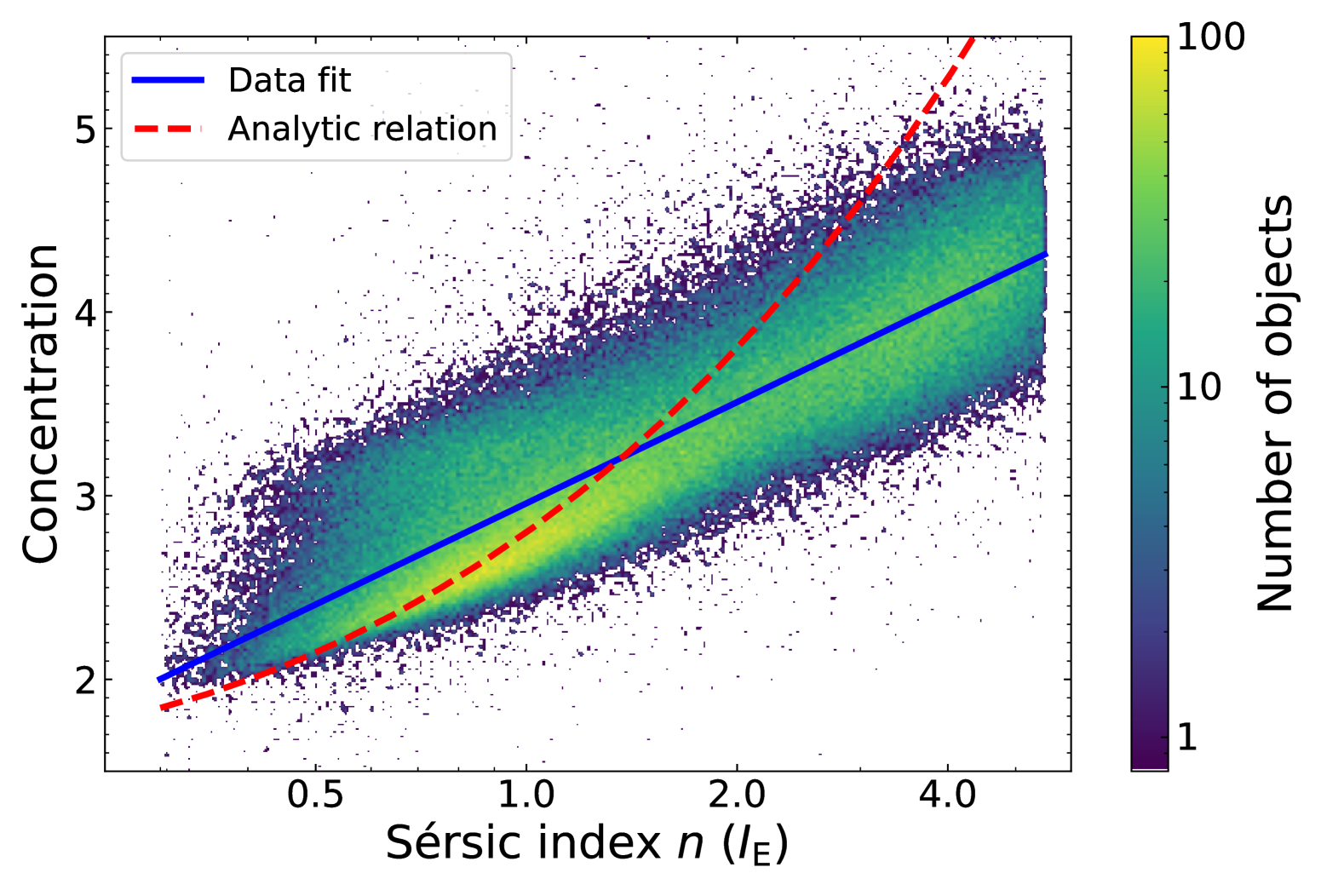
Figure 4: Concentration versus $n$ for Euclid galaxies with $I_{\scriptscriptstyle\rm E}$ $<\leavevmode\nobreak\ 21$. The blue solid line indicates a linear fit of the data, whereas the red line is an analytical relation for pure Sérsic profiles (see text).

The Concentration parameter, $C$, is measured as described in Conselice (2003, see details in ), and it measures how concentrated the light distribution of a galaxy is in its inner regions. Therefore, assuming that galaxies are well described by a Sérsic profile, one would expect a correlation between these two parameters, i.e., high $n$ and concentration values for early-type galaxies, lower values for later morphologies (see Andrae et al. 2011; Tarsitano et al. 2018; Wang et al. 2024). Figure 4 shows that this expected correlation is obtained in the Euclid morphological measurements for all galaxies with $I_{\scriptscriptstyle\rm E}<21$, presenting a Pearson correlation coefficient of $r=0.82$ between $C$ and $\operatorname{log_{10}}(n)$. Fitting a first degree polynomial for $C$ as a function of $\operatorname{log_{10}}(n)$ yields

$$C=2.97+1.81\operatorname{log_{10}}(n)\,,$$ (3)

with a $R^{2}$ score of 0.73, and a RMS dispersion of 0.32. This correlation, therefore, supports the reliability of both measures. Moreover, for a pure Sérsic profile, it is possible to compute analytically its Concentration and it only depends on $n$ (Graham & Driver 2005; Baes & Ciotti 2019). This relation is shown as a dashed red line in Fig. 4. We note that for $n\sim 1$ it goes through the high density of points with the lowest $C$ values around 2.5. We suggest that this high density area corresponds to disc-like galaxies, whereas other objects at similar $n$ but higher $C$ might host a weak bulge or bar, which is not fitted by the Sérsic profile but stills impact the concentration. For higher $n$ values, the analytical prediction leads to $C$ values well above what is measured because, while Sérsic fits are convolved by the PSF, the computation of $C$ does not take it into account and is therefore biased (the PSF spreads the light hence diminishes concentration). Combining the data fit and the analytical relation could allow one to derive $C$ values corrected for the PSF impact, as is done in Tarsitano et al. (2018).

5.3 Sérsic parameters versus Zoobot

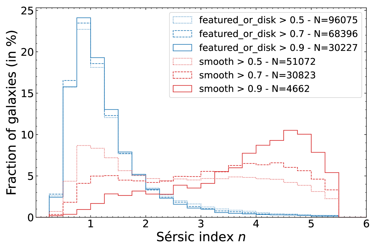
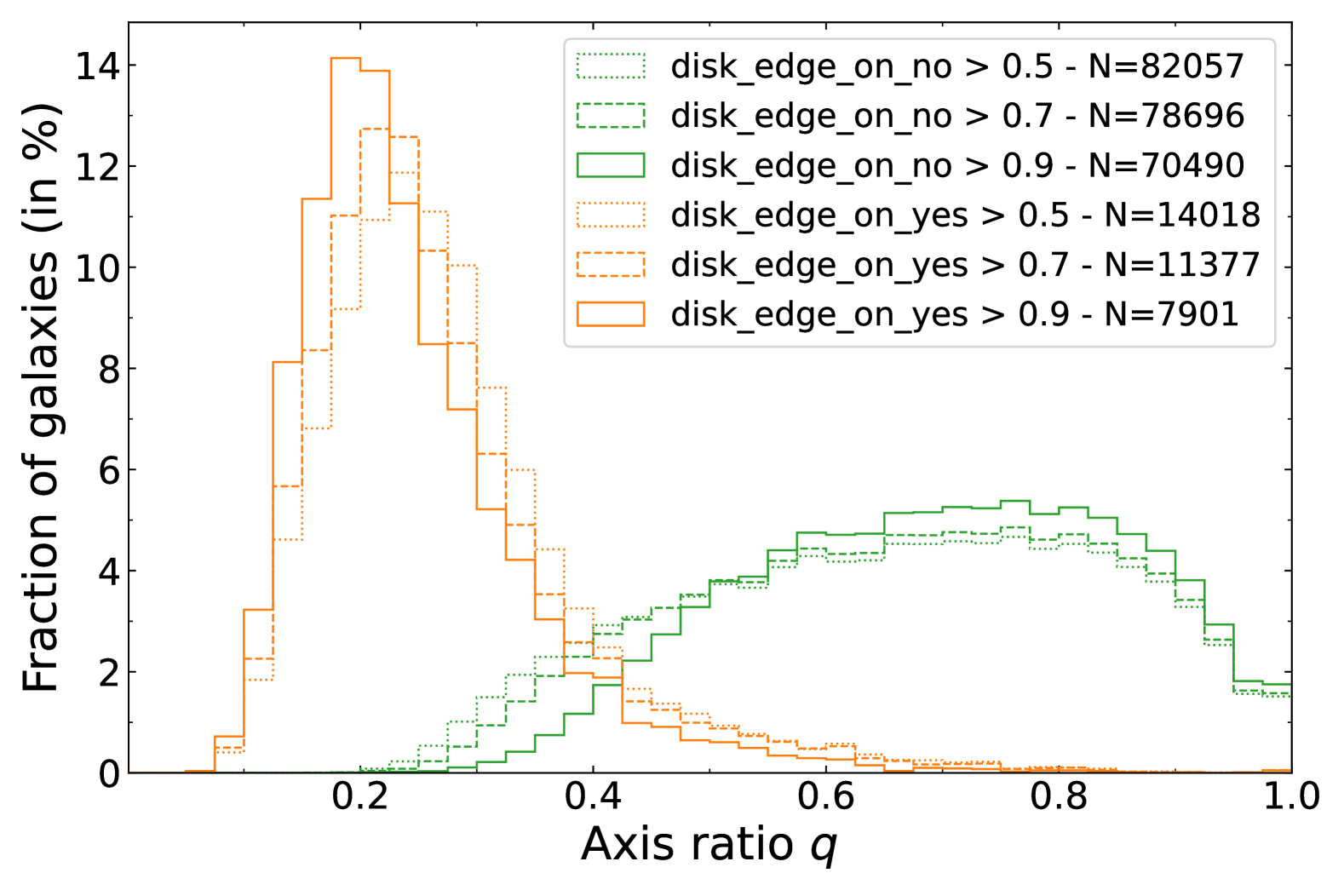
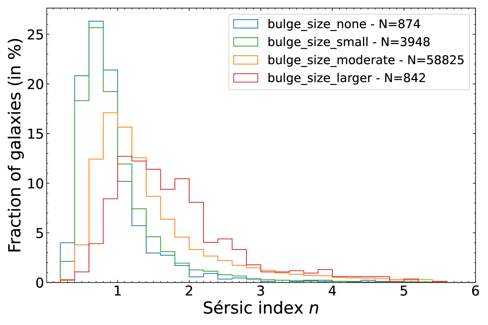
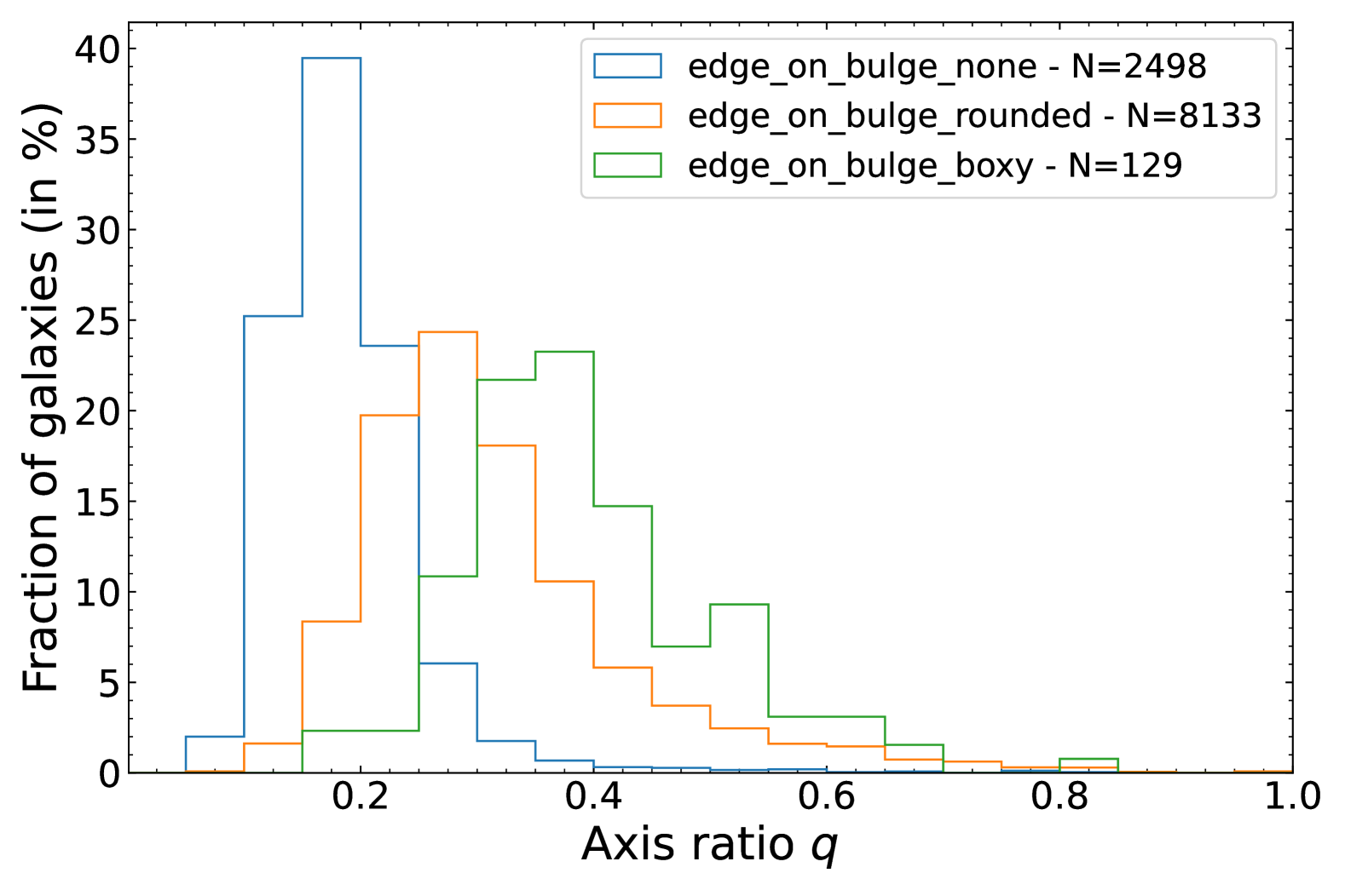
Figure 5: Distribution of Sérsic parameters measured on the VIS image for sub-samples of galaxies depending on their classification by the Zoobot labels, with different line styles corresponding to the different shares of expected votes predicted by Zoobot to consider that a galaxy falls into a certain category. Sample sizes are systematically indicated in the legend, and a 50% threshold of voters is adopted when not specified (bottom plots). Top-left: distribution of $n$ for galaxies classified as either smooth (red lines) or displaying a disc or features (blue lines) shows a clear dichotomy with the latter sample being almost exclusively made of galaxies with $n\sim 1$, whereas the former contains a lot of galaxies with high values of $n$ and increasingly so for higher selection threshold. Top-right: distribution of $q$ for disc galaxies depending if they are edge-on or not. Again, a clear bimodality appears, with low $q$ for edge-on galaxies and higher values spread across a wider interval for non-edge-on, hence from face-on to moderately inclined galaxies. Using higher thresholds reinforces this dichotomy. Bottom-left: Distribution for disc or featured galaxies of $n$ for different categories of Zoobot bulge sizes. Histograms shift to higher values of $n$ for larger relative bulge sizes. Bottom-right: Distribution of $q$ for edge-on disc galaxies, depending on if they display no bulge, a boxy bulge, or a rounded bulge. The presence of a bulge, either rounded or boxy, leads to higher $q$.

We next compare the results of Sérsic fits to machine-learning based labels obtained using Zoobot, which is presented in Euclid Collaboration: Walmsley et al. (2025). We follow the tree structure of the various questions asked to citizens and for which an expected fraction of voters was predicted by Zoobot. The sample used in this section corresponds to galaxies for which such labels are available, with $I_{\scriptscriptstyle\rm E}<20.5$ or a segmentation area larger than 1200 pixels (see Euclid Collaboration: Walmsley et al. 2025).

The top-left panel of Fig. 5 shows the distribution of $n$ for galaxies depending on whether they appear smooth (red curves), or whether they appear as a disc or display features (blue curves). We consider different shares of predicted votes (50%, 70%, and 90%, as dotted, dashed, and solid lines respectively) to consider that a galaxy falls into a category. The resulting number of galaxies for all samples are indicated in the figure insert. In all cases, the $n$ distribution for featured or disc galaxies peaks around 1, sharply decreasing for higher values of $n$, with a median of 1.1, and associated dispersion of 0.5 (estimated as half the 16-84th percentile range). This is the expected behaviour as disc-like galaxies are known to be preferably fitted by an exponential profile, corresponding to $n=1$. Using a more stringent share of voters slightly decreases the tail of high $n$ values with 90% quantiles of 2.5, 2.3, and 2.2 for the 50%, 70%, and 90% share of votes. Therefore, to benefit from larger statistics, selecting for disc or featured galaxies in the subsequent plots of this section is done using a predicted share of voters above 50%. Regarding galaxies voted as smooth, they should correspond to ellipticals, which are usually characterised by high $n$ (especially $n=4$, which is the de Vaucouleurs profile, de Vaucouleurs 1948). Again, we observe the expected trend as the distribution of $n$ includes higher $n$ galaxies than the disc or featured ones, or than the global distribution shown in the left panel of Fig. 1. However, here the chosen threshold has a significant impact on the resulting distribution of $n$, with median $n$ increasing from 2.5 to 3.3 and 4.0 for more stringent thresholds.

The top-right panel of Fig. 5 shows the distribution of $q_{\rm Sersic}$ for disc or featured galaxies depending if they were classified by Zoobot as being edge-on (orange) or not (green), still using the three thresholds of 50, 70, and 90% of expected votes. We observe again a striking consistency between the Sérsic parameters and Zoobot labels, since there is a clear dichotomy in the distributions of $q$ between the galaxies identified as edge-on or not, with median values of 0.26 and 0.67, and dispersions of 0.09 and 0.20, respectively (using the 50% threshold). Moreover, the two histograms barely overlap for intermediate $q\sim 0.4$, with 90% of not edge-on discs having $q>0.4$ whereas 88% of edge-on ones have $q<0.4$. Requiring higher shares of votes to decide if a galaxy is edge-on or not slightly reinforces this separation between the two histograms, with, for instance, respective medians of 0.22 and 0.70 using a 90% threshold, but at the expense of statistics. Furthermore, if edge-on discs are expected to have minimal values of $q$, the presence of a bulge “bulging out” from the disc results in a modelled $q$ higher than the actual disc $q$, as shown by Q25a. This would explain the tail of higher $q$ values. This hypothesis is confirmed in the bottom-right panel of Fig. 5 using the subsequent Zoobot question regarding the presence of a bulge for galaxies selected as disc or featured, and as edge-on (always using a 50% threshold). Indeed, the resulting $q$ distributions show that in the absence of a bulge, it peaks around a median value of 0.18, with a dispersion of 0.05, and displays a sharper decrease than for all edge-on galaxies, with only 4% of galaxies having $q>0.3$. The presence of a rounded or boxy bulge shifts the distribution towards higher $q$, with respective medians of 0.29 and 0.37, as well as 46% and 83% of the subsamples displaying $q>0.3$.

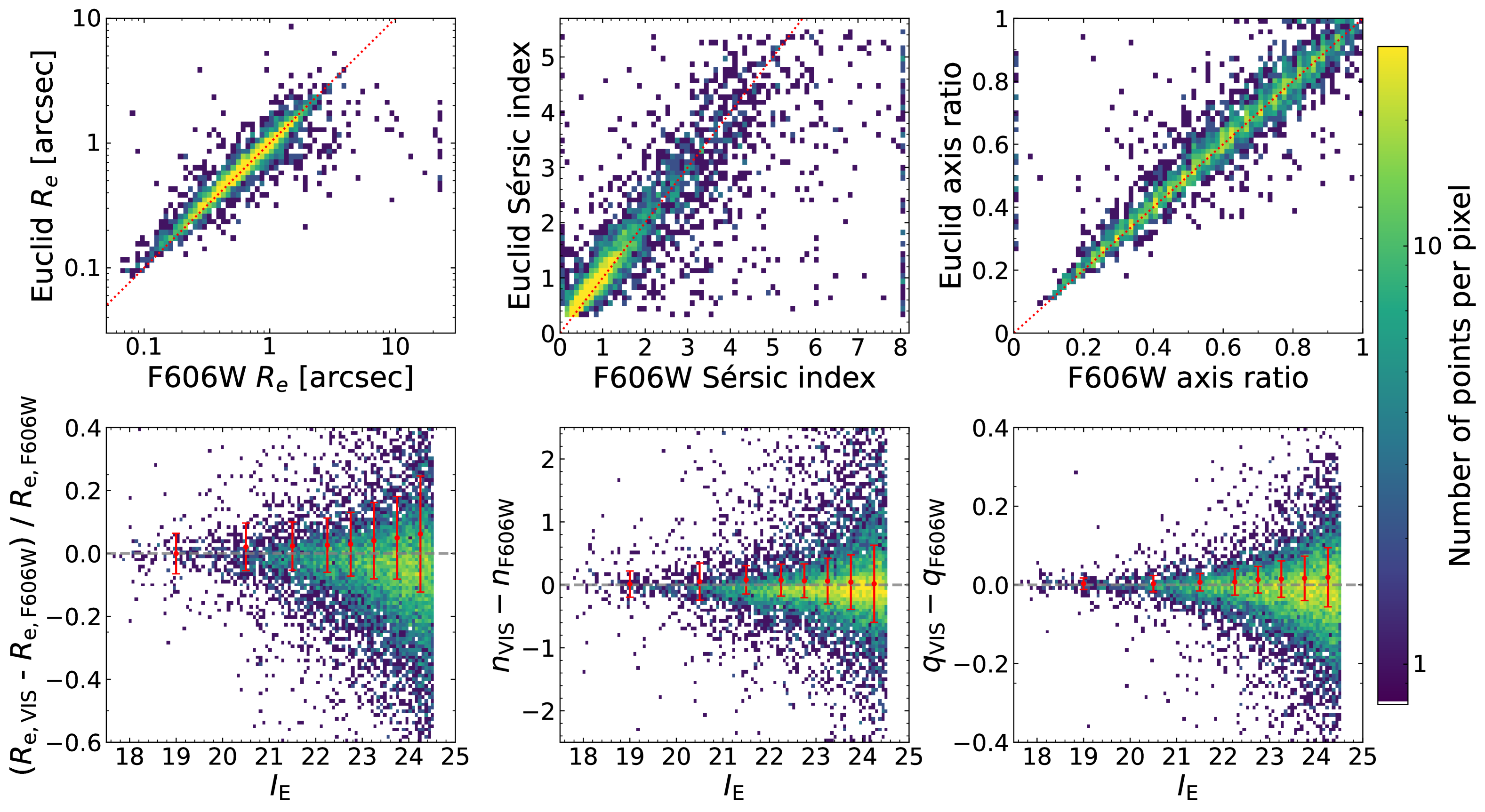
Figure 6: Comparison between Euclid and ACS-GC derived parameters. The top line shows the $R_{\mathrm{e}}$, $n$ and $q$ for galaxies with $I_{\scriptscriptstyle\rm E}<23$. The bottom line includes galaxies with $I_{\scriptscriptstyle\rm E}<24.5$ and shows the relative difference or difference between the same set of parameters as a function of the magnitude. The red points and error bars indicate median values and associated dispersions computed in bins of magnitude.

Finally, in the bottom-left panel of Fig. 5 we show the $n$ distributions of galaxies that are featured or discs, and not edge-on, depending on their predicted bulge size, using for all labels a threshold of 50% of predicted votes. The answers bulge_size_large and bulge_size_dominant have been grouped together as bulge_size_larger since they were rarer and because galaxies with very few expected votes in the three smaller bulge sizes often have split votes between these two larger categories, so none of them were above the 50% threshold, but the expected votes repartition still indicated that Zoobot predicted a large bulge within these galaxies. Since the single Sérsic profile fits both the light of the bulge and the disc, the more important the bulge flux is compared to the total galaxy flux, the higher the fitted $n$ should be. The current Zoobot question measures rather the ratio between the bulge and disc sizes, but this quantity is correlated to the bulge-to-total light ratio (Quilley & de Lapparent 2023). The distributions observed in the bottom-left panel of Fig. 5 correspond to this prediction, with overall larger values of $n$ for larger bulge sizes predicted by Zoobot: the successive median values are 0.81, 0.85, 1.21, 1.60. The share of galaxies within the tail of high $n$ also increases, with 3.2%, 3.6%, 11.4%, and 15.9% of galaxies with $n>2.5$, respectively. The lack of a significant difference between the bulge_size_none and bulge_size_small, especially compared to the gap seen between bulge_size_small and bulge_size_moderate can be explained by the fact that bulges have to reach some fraction of the total flux in order to impact and steepen the single Sérsic fits, otherwise they are not modelled, as shown in Q25a.

Overall, the descriptions of galaxy morphology provided by parametric model-fitting and by machine-learning methods are consistent with each other, and the observed trends are those expected. This analysis also demonstrates the potential of using both information jointly.

5.4 Comparison with previous surveys

In order to confirm the validity of Sérsic parameters derived in the Euclid pipeline, we compare them to previous measurements. We use the Advanced Camera for Surveys General Catalog (Griffith et al. 2012, ACS-GC hereafter), containing the GEMS field, which overlaps with the EDF-F. In this case the Sérsic fits were performed using HST images in the F606W band, with a pixel scale of $0.\mathrm{″}03$, and using GALAPAGOS.

We perform a cross-match between our catalogue and ACS-GC. Two galaxies are considered to be the same object if the angular distance between them is smaller than $1.\mathrm{″}0$. We find 11 884 galaxies with $I_{\scriptscriptstyle\rm E}<24.5$ and 3805 galaxies with $I_{\scriptscriptstyle\rm E}<23$ in the 0.21 deg² of overlapping area. Figure 6 shows the comparison between the Sérsic structural parameters derived from Euclid and ACS-GC. The respectively derived $n$ and $q$ values are in agreement with each other, with median differences compatible with zero: they are below 0.1 for $n$ and below 0.01 for $q$. The $R_{\rm e}$ values display an offset, with VIS radii being larger than the ACS-GC radii, and increasingly so for fainter magnitudes: the median relative difference remains below 3% for $I_{\scriptscriptstyle\rm E}<23$ and increases to 6% at the faintest magnitudes. This offset is likely to be a consequence of the different depths and resolutions of the images used in both analyses (George et al. 2024). For all three parameters, the scatter increases with magnitude.

The agreement found here, as well as the evidence detailed in the previous subsections, confirms the robustness of the Sérsic fits implemented within the Euclid pipeline.

6 Variation of structural parameter with wavelength: colour gradients

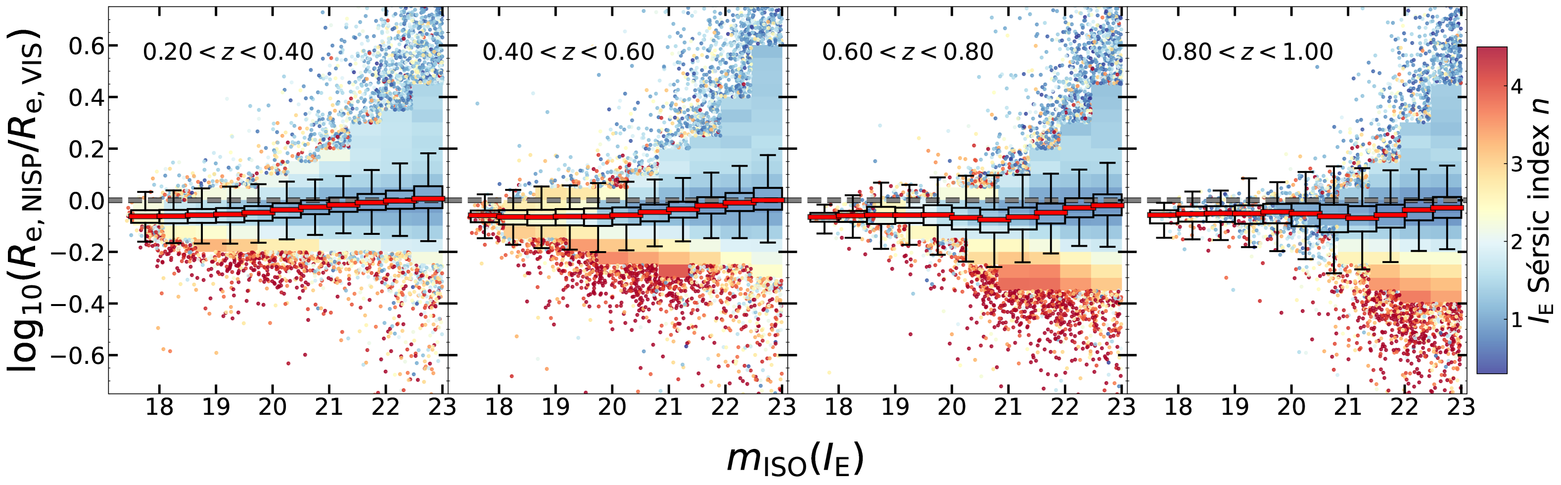
Figure 7: The ratio between effective radius based on the common Sérsic model for three NISP images ($R_{\mathrm{e,\,NISP}}$) and that from the Sérsic fit to the VIS image ($R_{\mathrm{e,\,VIS}}$) as a function of isophotal VIS magnitude. The four panels correspond to the redshift bins we use to trace evolutionary trends in Sect.  7. The 2-dimensional (2D) histogram in each panel are colour-coded by the median $n_{\mathrm{VIS}}$ for galaxies in a given $[\Delta m_{\rm ISO}(I_{\scriptscriptstyle\rm E})=0.5$, $\Delta\log(R_{\mathrm{e,\,NISP}}/R_{\mathrm{e,\,VIS}})=0.05]$ pixel. The 2D histogram includes pixels with $N>100$ galaxies. In more sparsely populated regions we instead display individual galaxies colour-coded by their $n_{\mathrm{VIS}}$. The box-and-whisker diagrams show median values (red solid lines), interquartile range (IQR, boxes) and the extent of the 1.5 IQR range above the 75th and below the 25th percentile (whiskers) for $R_{\mathrm{e,\,NISP}}/R_{\mathrm{e,\,VIS}}$ in $\Delta m_{\rm ISO}=0.5$ bins of isophotal $I_{\scriptscriptstyle\rm E}$. The grey dashed line corresponds to the constant ratio of $R_{\mathrm{e,\,NISP}}/R_{\mathrm{e,\,VIS}}=1$.

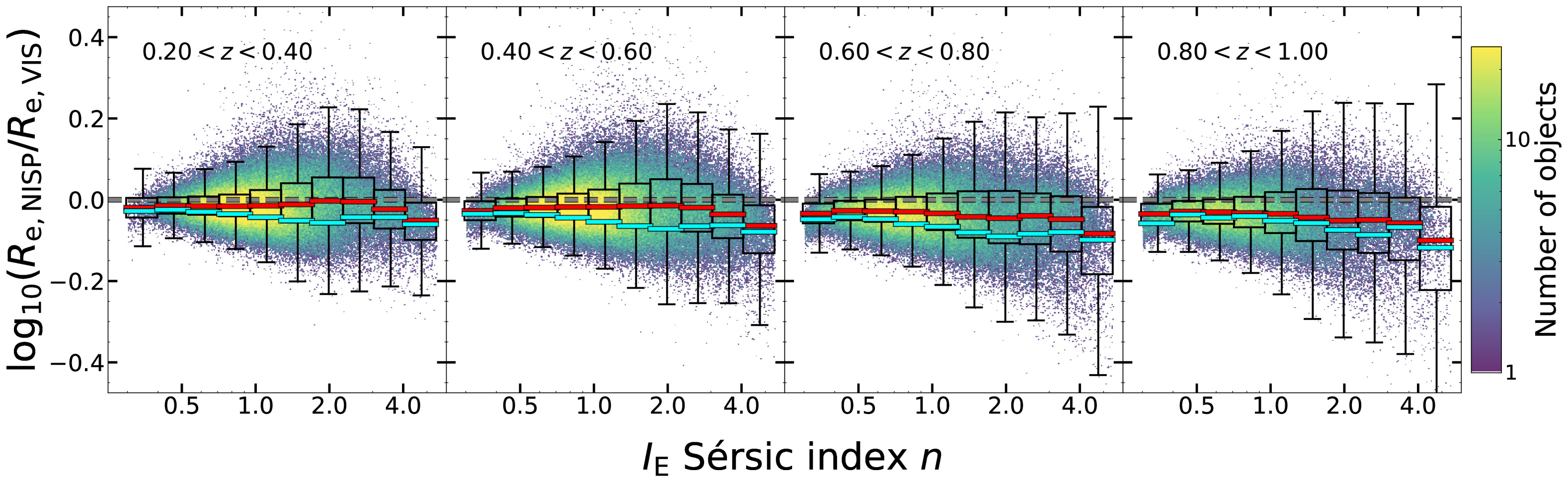
Figure 8: NISP-to-VIS $R_{\mathrm{e}}$ ratio as a function of $n_{\mathrm{VIS}}$ for galaxies with isophotal VIS magnitude $m_{\rm ISO}(I_{\scriptscriptstyle\rm E})<23$. The four panels correspond to the same redshift bins as in Fig. 7. In each panel density map is colour-coded by the number of galaxies in a given pixel. The box-and-whisker diagrams show median values (red lines), interquartile range (IQR, boxes) and the extent of the 1.5 IQR range above the 75th and below the 25th percentile (whiskers) for $R_{\mathrm{e,\,NISP}}/R_{\mathrm{e,\,VIS}}$ ratios in 10 bins of $n_{\mathrm{VIS}}$. For comparison, we show median $R_{\mathrm{e,\,NISP}}/R_{\mathrm{e,\,VIS}}$ ratios in the same $n_{\mathrm{VIS}}$ for galaxies with the isophotal VIS magnitude $m_{\rm ISO}(I_{\scriptscriptstyle\rm E})<21$ (cyan solid lines). The grey dashed line corresponds to the constant ratio of $R_{\mathrm{e,\,NISP}}/R_{\mathrm{e,\,VIS}}=1$.

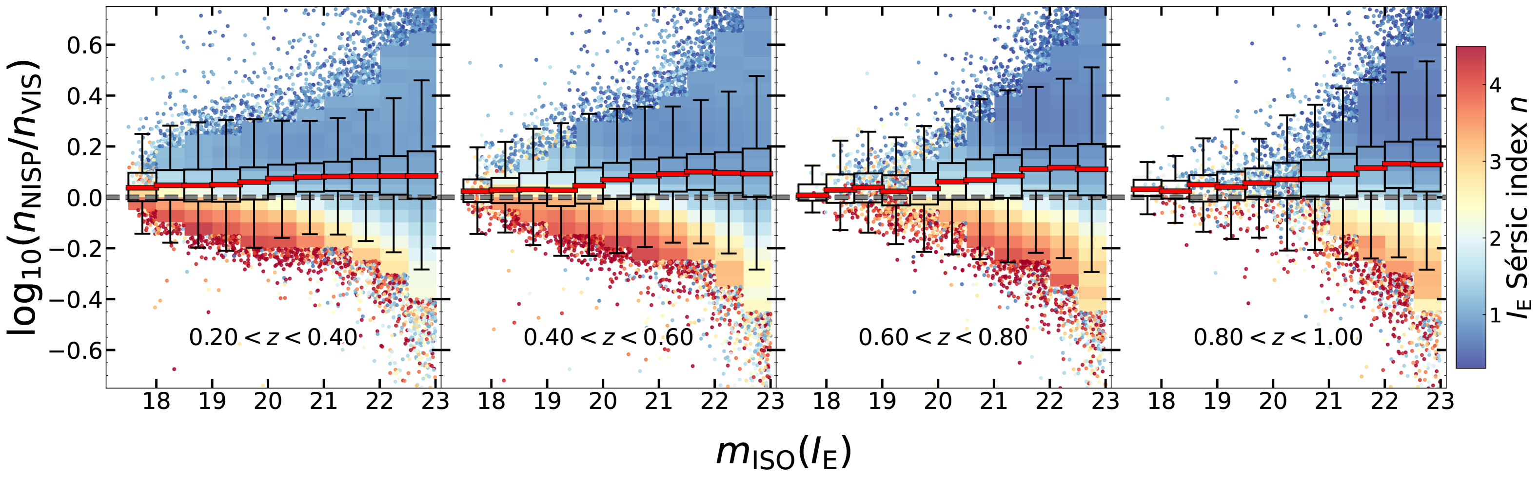
Figure 9: Equivalent to Fig. 7 but for the ratio of $n$ in NISP and VIS bands as a function of galaxy isophotal VIS magnitude.

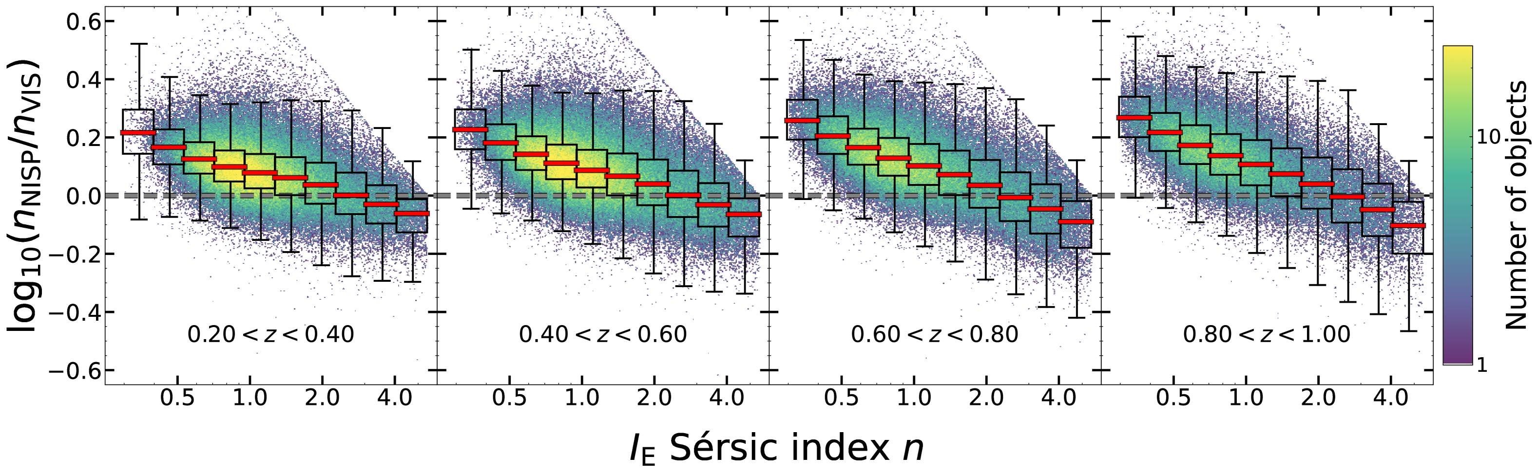
Figure 10: Equivalent to Fig. 8 but for the ratio of $n$ in NISP and VIS bands as a function of $n_{\mathrm{VIS}}$. We omit the binned median values of the index ratio for $m_{\rm ISO}(I_{\scriptscriptstyle\rm E})<21$ sample because they are nearly identical to the median values for the parent sample with $m_{\rm ISO}(I_{\scriptscriptstyle\rm E})<23$.

Table 1: Redshift evolution of ratios of the structural parameters fitted

			Redshift
			$0.2<z<0.4$	$0.4<z<0.6$	$0.6<z<0.8$	$0.8<z<1$
$\frac{R_{\mathrm{e,\,NISP}}}{R_{\mathrm{e,\,VIS}}}$	$I_{\scriptscriptstyle\rm E}<21$	$n_{\mathrm{VIS}}<2.5$	$0.914^{+0.001}_{-0.001}$	$0.891^{+0.001}_{-0.001}$	$0.859^{+0.002}_{-0.002}$	$0.889^{+0.004}_{-0.005}$
		$n_{\mathrm{VIS}}>2.5$	$0.894^{+0.001}_{-0.002}$	$0.856^{+0.003}_{-0.002}$	$0.821^{+0.005}_{-0.004}$	$0.820^{+0.020}_{-0.008}$
	$I_{\scriptscriptstyle\rm E}<23$	$n_{\mathrm{VIS}}<2.5$	$0.968^{+0.001}_{-0.001}$	$0.959^{+0.001}_{-0.001}$	$0.940^{+0.001}_{-0.001}$	$0.926^{+0.001}_{-0.001}$
		$n_{\mathrm{VIS}}>2.5$	$0.845^{+0.002}_{-0.002}$	$0.919^{+0.001}_{-0.002}$	$0.888^{+0.002}_{-0.002}$	$0.866^{+0.003}_{-0.003}$
$\frac{n_{\mathrm{NISP}}}{n_{\mathrm{VIS}}}$	$I_{\scriptscriptstyle\rm E}<21$	$n_{\mathrm{VIS}}<2.5$	$1.230^{+0.002}_{-0.002}$	$1.268^{+0.002}_{-0.002}$	$1.250^{+0.006}_{-0.004}$	$1.220^{+0.010}_{-0.010}$
		$n_{\mathrm{VIS}}>2.5$	$0.939^{+0.003}_{-0.002}$	$0.947^{+0.002}_{-0.002}$	$0.963^{+0.005}_{-0.005}$	$0.950^{+0.010}_{-0.001}$
	$I_{\scriptscriptstyle\rm E}<23$	$n_{\mathrm{VIS}}<2.5$	$1.231^{+0.001}_{-0.001}$	$1.275^{+0.001}_{-0.001}$	$1.345^{+0.001}_{-0.001}$	$1.401^{+0.002}_{-0.002}$
		$n_{\mathrm{VIS}}>2.5$	$0.934^{+0.002}_{-0.002}$	$0.929^{+0.002}_{-0.002}$	$0.902^{+0.002}_{-0.003}$	$0.893^{+0.004}_{-0.003}$

The colours of galaxies vary spatially across their extent, with, in most cases, the inner region of the bulge showing redder colour than the disc (Möllenhoff 2004; Vika et al. 2014; Kennedy et al. 2016; Casura et al. 2022), but the variations go beyond that dichotomy and also arise within bulges or discs (Natali et al. 1992; Balcells & Peletier 1994; de Jong 1996; Pompei & Natali 1997, Q25a). These colour gradients are the result of stellar population (age and metallicity) gradients within galaxies and differential dust attenuation. It is estimated that the relative contribution of stellar and dust gradients to the measured colour gradient is of the order of $80\%$ and $20\%$ respectively (Baes et al. 2024). Therefore, the observation and quantification of colour gradients provide constraints for the evolutionary scenarios of the galaxy stellar mass build-up. Moreover, studies of galaxy colour gradients provide a valuable insight into biases affecting the shear measurements for weak lensing analysis (Semboloni et al. 2013; Er et al. 2018).

In photometric studies, spatial variations are mostly investigated radially to test the inside-out or outside-in mass assembly models (e.g., Avila-Reese et al. 2018). This can be done using a series of aperture magnitudes of increasing radius or, in the present case, modelling galaxy 2D profiles with the same analytic function in different bands, and inspecting how the parameters of the model vary between bands. For Sérsic profiles, variations in R_e and $n$ with the observing band are indicative of colour gradients.

In order to assess Euclid’s ability to detect colour gradients in large galaxy samples, we take advantage of the fact that the present data release provides two sets of Sérsic parameters, one in $I_{\scriptscriptstyle\rm E}$ and one common to the three NISP bands. We note that the previous study of Q25a on the Euclid ERO data has shown that the structural parameters of a common model for the $Y_{\scriptscriptstyle\rm E}$, $J_{\scriptscriptstyle\rm E}$, and $H_{\scriptscriptstyle\rm E}$ bands lead to values close to an independent model for the $J_{\scriptscriptstyle\rm E}$ image, due to its central wavelength position between $Y_{\scriptscriptstyle\rm E}$ and $H_{\scriptscriptstyle\rm E}$ bands and the smoothness of the variation of the structural parameters with wavelength in these neighbouring bands.

Figures 7–10 show trends in structural parameter ratios $R_{\mathrm{e}}$ and $n$ with $I_{\scriptscriptstyle\rm E}$ and $n_{\rm VIS}$ across four $\Delta z=0.2$ redshift bins, which match the intervals explored in Sect. 7. Table 3 lists median values for different sample subsets in these bins. Smaller R_e and more concentrated profiles (higher $n$) in NISP compared to VIS are both indicative of redder-inside colours (and vice versa).

For the sample described in Sect. 2, the median Sérsic $R_{\rm e}$ in combined NISP bands is about $\sim 10\%$ smaller than the R${}_{\rm e,\,VIS}$ for all galaxies at $z<1$ up to $I_{\scriptscriptstyle\rm E}$ $\lesssim 21$ (red solid lines in Fig. 7, see also Table 3). The trend significantly weakens at fainter magnitudes ($I_{\scriptscriptstyle\rm E}$ $>21$) in the $0.2<z<0.4$ and $0.4<z<0.6$ intervals, whereas it increases at magnitudes brighter than $I_{\scriptscriptstyle\rm E}\approx 19.5$ in the two higher redshift intervals, then weakens starting from $I_{\scriptscriptstyle\rm E}\approx 21$. A previous analysis of the Euclid ERO data with two-component fits to galaxy light profiles showed that the decrease in $R_{\mathrm{e}}$ with the wavelength of observation is a combination of two effects: bulge-disc colour dichotomy and the colour gradients within disc component (Q25a), affecting the dominating population of spiral galaxies detected in the present sample. Thus, the ratio between effective radii in observed NISP and VIS ($R_{\mathrm{e,\,NISP}}/R_{\mathrm{e,\,VIS}}$) in Fig. 7 traces, on average, a more compact structure of longer-wavelength light profiles for all galaxies with $I_{\scriptscriptstyle\rm E}$ $\leq 21$, that can be reliably fitted with two-component (bulge+disc) Sérsic models (see Euclid Collaboration: Bretonnière et al. 2023; Q25a).

At fixed magnitude, the ratio distribution follows a trend with $n_{\mathrm{VIS}}$ (Fig.  7). For $I_{\scriptscriptstyle\rm E}$ $\lesssim 20$ and $z<0.8$, a broad range of median $R_{\mathrm{e,\,NISP}}/R_{\mathrm{e,\,VIS}}$ values ([0.4, 1.6]) of galaxies with $n\gtrsim 2.5$ envelops the $R_{\mathrm{e,\,NISP}}/R_{\mathrm{e,\,VIS}}\lesssim 1$ for disc ($n\lesssim 1$) galaxies. Densely populated cells with low median values of $n_{\mathrm{VIS}}$ drive the median ratio of $\approx 0.87$ at these magnitudes. At $I_{\scriptscriptstyle\rm E}$ $\sim 21$, galaxies with $n\gtrsim 2.5$ have $R_{\mathrm{e,\,NISP}}$ up to 60% smaller than $R_{\mathrm{e,\,VIS}}$. In contrast, the $R_{\mathrm{e,\,NISP}}$ of disc galaxies ($n\lesssim 1$) in the same $I_{\scriptscriptstyle\rm E}$ and redshift bins can be 2.5 times larger than $R_{\mathrm{e,\,VIS}}$. As in brighter magnitude bins, $n\sim 1$ (hence likely spiral) galaxies dominate the most populated cells at $I_{\scriptscriptstyle\rm E}$ $\sim 21$ and drive the median ratio of radii in two (sets of) bands (Table 3).

Combined magnitude bins show that the median ratio of galaxy $R_{\mathrm{e}}$ in the two observed wavelength regimes depends mildly on $n_{\rm VIS}$ (Fig. 8). The median offset between $R_{\mathrm{e,\,NISP}}/R_{\mathrm{e,\,VIS}}$ ranges from approximately $-5\%$ to $-10\%$ (of $R_{\mathrm{e,\,VIS}}$) for galaxies with $I_{\scriptscriptstyle\rm E}$ $<23$ and $n_{\mathrm{VIS}}$ from about $\sim 1$ to 4, respectively (red solid lines in Fig. 8, Table 3). Since the median ratio of the two radii at fixed $n$ is driven by the most numerous fainter galaxies (see the distribution of cells in Fig. 7), and because both simulated images and the analysis of ERO data indicate that the bulge-disc decomposition of Euclid galaxies becomes challenging at $I_{\scriptscriptstyle\rm E}\geq 21$ (Euclid Collaboration: Bretonnière et al. 2023; Q25a), we also explore median values as a function of $n$ for the $I_{\scriptscriptstyle\rm E}$ $<21$ sample (cyan lines in Fig. 8, Table 3). For this brighter subset, the median $R_{\mathrm{e,\,NISP}}/R_{\mathrm{e,\,VIS}}$ ratio is below the value for the parent sample in all $n$ bins across the redshift interval we probe, and the pattern of variations with $n_{\mathrm{VIS}}$ is similar between the four redshift intervals. The larger difference between two sets of ratios at from $n\sim 1$ to $n\sim 4$, and especially around $n\sim 2$ highlights the average redder-inside colour gradient of galaxies that can be reliably fitted by the sum of bulge and disc profiles. Thus Euclid Q1 data set reveals trends in galaxy structural properties that will inform future studies using more detailed parametric 2D models.

The Sérsic index of galaxies in our sample also changes with the observed wavelength range. Figure 9 illustrates the trend in the NISP-to-VIS $n$ ratio ($n_{\mathrm{NISP}}/n_{\mathrm{VIS}}$) with the galaxy isophotal $I_{\scriptscriptstyle\rm E}$ in the four $z<1$ redshift bins explored. The median values of this ratio (red solid lines) consistently exceed unity (grey dashed lines), with the profile concentration index measured in combined NISP bands being between $\sim$10% and 30% larger than the equivalent measurement in VIS band for $I_{\scriptscriptstyle\rm E}$ $<23$ galaxies (Table 3). We note that the same trend has been observed for galaxies at $0.5<z<3$ in Martorano et al. (2023) using Sérsic fits on JWST images.

At a fixed $I_{\scriptscriptstyle\rm E}$, the distribution of individual $n_{\mathrm{NISP}}/n_{\mathrm{VIS}}$ ratios is a function of $n_{\mathrm{VIS}}$ (Fig. 9). The most centrally concentrated VIS light profiles ($n_{\mathrm{VIS}}\gtrsim 2.5$) exhibit NISP profiles with up to $\sim 40\%$ and to $\sim 60\%$ (for the $I_{\scriptscriptstyle\rm E}$ $<21$ subset and for the full $I_{\scriptscriptstyle\rm E}$ $<23$ sample) smaller $n$. Together with, on average, smaller R${}_{\mathrm{e,\,NISP}}$ in galaxies with centrally concentrated VIS light profiles from Fig.  7, this trend could illustrate the build-up of outer halos around central bulges in these systems. In contrast to galaxies with the most concentrated VIS light profile, the majority of disc galaxies ($n_{\rm VIS}<2$) have more centrally concentrated NISP profiles, with $n_{\rm NISP}$ up to $\times$ 2.5 or up to four times larger (for the $I_{\scriptscriptstyle\rm E}$ $<21$ subset and for the full $I_{\scriptscriptstyle\rm E}$ $<23$ sample, respectively) than $n_{\rm VIS}$. The median values of the $n_{\mathrm{NISP}}/n_{\mathrm{VIS}}$ in Table 3 quantify further the difference between $n_{\mathrm{VIS}}<2.5$ and $n_{\mathrm{VIS}}>2.5$ systems. This trend is expected if combined NISP images are more sensitive to the redder central (bulge-like, $n\sim 4$) than VIS. However, we note that the highest ratio ($n_{\rm NISP}\gtrsim 2.5\,n_{\rm VIS}$) are here attributed to galaxies with $n_{\rm VIS}<1$ (dark-blue cells in Fig.  9).

We next combine all $I_{\scriptscriptstyle\rm E}$ $<23$ bins to explore the trend in $n$ ratio with $n_{\mathrm{VIS}}$ in Fig. 10. Galaxies in our sample follow the same median trend of decreasing $n_{\mathrm{NISP}}/n_{\mathrm{VIS}}$ ratio with increasing $n_{\mathrm{VIS}}$ in all four redshift bins explored. The majority of galaxies in our parent sample are disc-dominated ($n_{\mathrm{VIS}}<2$, Fig. 1), showing more concentrated NISP profiles ($n_{\mathrm{NISP}}>n_{\mathrm{VIS}}$, Fig. 9). For disc-dominated galaxies with $n_{\mathrm{VIS}}\sim 1$, $n_{\mathrm{NISP}}$ are roughly 25% and 40% larger than $n_{\mathrm{VIS}}$ in $z\sim 0.3$ and $z\sim 0.9$, respectively. For extreme $n_{\mathrm{VIS}}\lesssim 0.5$ values, this difference increases to $\sim 65\%$ at $0.2<z<0.6$ and $\sim 85\%$ at $0.6<z<1$, respectively.

The decreasing trend in the $n_{\mathrm{NISP}}/n_{\mathrm{VIS}}$ ratio with $n_{\mathrm{VIS}}$ is significant, exceeding the median trend with magnitude illustrated in Fig. 9. We note again, however, that the large differences at very low $n_{\mathrm{VIS}}$ values do not imply a drastic change in morphology from disc-like to bulge-like between VIS and NISP. Nevertheless, the $n_{\mathrm{NISP}}/n_{\mathrm{VIS}}$ ratio $>1$ for all galaxies with $n_{\mathrm{VIS}}<2.5$ (quantified also in Table 3), suggest that a more concentrated inner structure (i.e., bulge) affects single Sérsic light profiles of disc-dominated galaxies at longer wavelengths, regardless of the exact rest-frame wavelength probed with VIS and NISP. In contrast, the median ratios close to unity for galaxies with significant bulge-like structure ($n_{\mathrm{VIS}}\gtrsim 2.5$) suggest more subtle effects for these early-type galaxies, in agreement with Q25a.

Based on the Euclid Q1 galaxy data set and their single-Sérsic profile fits, a combination of the median trend of larger $n$ in NISP bands with respect to VIS ($n_{\mathrm{NISP}}/n_{\mathrm{VIS}}>1$, Fig. 10) for galaxies with prominent disc component ($n_{\mathrm{VIS}}<2$) and the median $R_{\mathrm{e,\,NISP}}/R_{\mathrm{e,\,VIS}}\lesssim 1$ trend (Fig. 8) supports an inside-out mass assembly scenario (e.g., Muñoz-Mateos et al. 2007; Pezzulli et al. 2015; Baker et al. 2024). Furthermore, the median $n$ ratio close to unity and the smaller $R_{\mathrm{e,\,VIS}}$ for bulge-dominated ($n_{\rm VIS}>2.5$) galaxies align with the predictions of the “two-phase” formation scenario with a rapid early phase ($z>2$) of in-situ star-formation followed by an extended phase of (gas and/or star) accretion (e.g., Naab et al. 2009; Oser et al. 2010; Hilz et al. 2012; Rodriguez-Gomez et al. 2016). Statistical galaxy samples from future Euclid data releases, spanning a broad range in redshift, stellar mass, star-formation activity, and with structural parameters for both the bulge and disc component, will be ideal platforms for probing multiple scenarios of galaxy mass assembly.

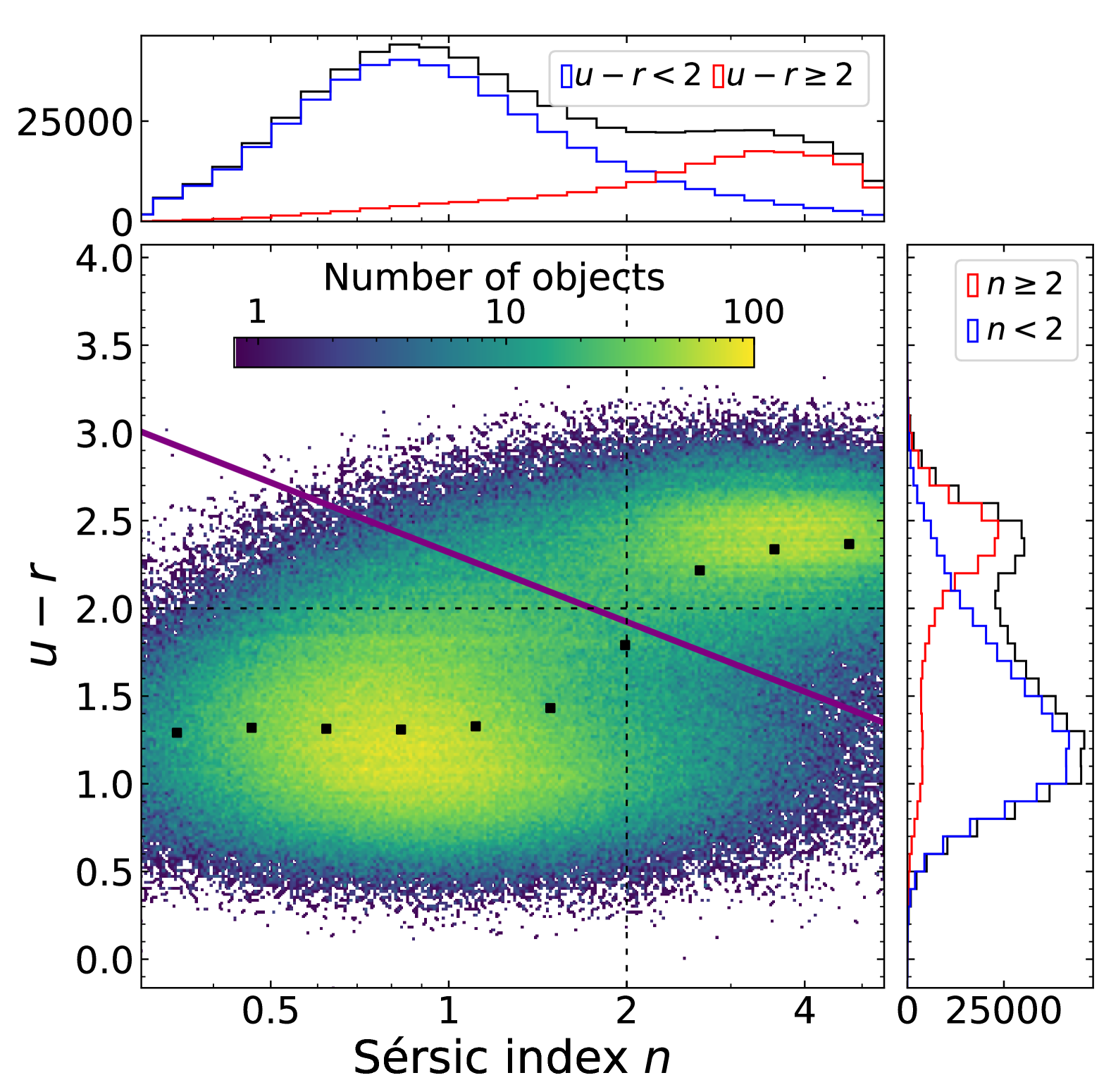
Figure 11: Rest-frame $(u-r)$ colour versus $n$ for all galaxies with $I_{\scriptscriptstyle\rm E}$ $\leq 23$. Black squares indicate the running median colour in bins of $n$. Histograms on the right and top plots show the 1D distributions for each quantity. A clear colour–morphology bimodality in the galaxy populations is displayed, with two density peaks corresponding respectively to blue spiral galaxies with $n\sim$ 1 and $(u-r)\sim$ 1.2, and red early-type galaxies of $n\sim$ 4 and $(u-r)\sim$ 2.4. We use this plane to define the early- and late-type galaxies sub-samples, separated by the solid purple line.

We also emphasise that for galaxies at different redshifts, variations in $R_{\mathrm{e}}$ and $n$ across bands have different implications, since galaxies at different redshifts are fitted with single Sérsic profiles in different rest-frame bands. Therefore the similar pattern of $R_{\mathrm{e}}$ and $n$ ratios between the observed VIS and NISP bands measured must be interpreted with caution, the wavelength and redshift effects being entangled. For instance, at $z\approx 1$, the $I_{\scriptscriptstyle\rm E}$ band probes mostly wavelengths below $4000\,\AA$ whereas the NISP central band $J_{\scriptscriptstyle\rm E}$ probes roughly the 6000–7500 $\AA$ range. As bulge-to-total ratios that contribute to single-Sérsic gradients increase more strongly from UV to optical than from optical to near-infrared, in the absence of redshift evolution, a steeper gradient is therefore expected in the $z\sim 0.8$ –1.0 subsample (hence ratios of $R_{\mathrm{e}}$ and $n$ deviating more from 1) than for the lowest redshift subsample. The fact that such an effect is unseen does not exclude redshift evolution in the galaxy internal colour distributions between $z\approx 0$ to $1$, as it could be compensated by the effect of the shift in rest-frame bandwidth. Interpreting the variations of the colour gradients requires precise redshift determination and careful analysis of stellar populations and dust effects, as well as the sample selection effects and the different PSF and angular resolution in VIS compared to NISP. A detailed study is left for future work.

7 Variations of scaling-laws with morphology for redshifts $z<1$

In this section, we investigate how morphology correlates with the stellar mass and star-forming state of galaxies by examining the position of different galaxy morphologies across well-established scaling relations, namely the the size–mass relation and the star-formation rate (SFR)–mass relation, which highlights the Main Sequence of star-forming galaxies. Redshifts, absolute magnitudes, stellar masses, and SFRs used in this section are extracted from the catalogue of physical parameters presented in Euclid Collaboration: Tucci et al. (2025). These quantities were derived by the SED-fitting of Euclid near-IR photometry and optical ground-based external data.

7.1 Colour-morphology bimodality

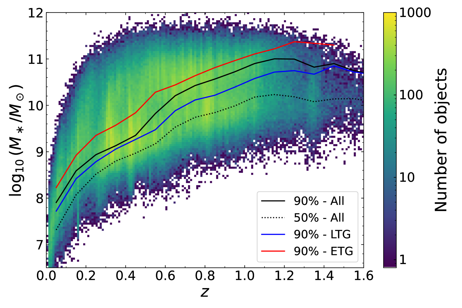
Figure 12: Stellar mass versus photometric redshift of galaxies with $I_{\scriptscriptstyle\rm E}$ $\leq 23$. Following the methodology of Pozzetti et al. (2010), we compute the mass completeness limits of the full sample at the 90% and 50% levels, shown as solid and dotted black lines respectively, as well as for the sub-samples of late and early-type galaxies, with their 90% mass completeness limits shown in solid blue and red lines, respectively.

The colour bimodality of galaxy populations (Strateva et al. 2001; Baldry et al. 2004) shows a clear correlation between colour and morphology: early-type galaxies are predominantly red, whereas later types are mostly blue. However, further investigation by Quilley & de Lapparent (2022), locating all the morphological types in the colour–mass diagram, showed that this connection goes beyond a simple bimodality, with the Hubble sequence monotonously spanning this plane. Figure 11 shows the $(u-r)$ distribution with $\operatorname{log_{10}}(n)$. This colour is obtained from the absolute magnitudes derived in these bands from the SED-fitting of Euclid and external photometry (see Euclid Collaboration: Tucci et al. 2025). A colour–concentration bimodality emerges, with blue galaxies having mostly $n\sim$ 1, typical of the exponential profiles of discs, whereas red galaxies display $n\sim$ 4, more indicative of an early-type morphology (elliptical or lenticular). This is in agreement with the previous analysis of Allen et al. (2006), which first highlighted this 2D colour–concentration bimodality. We use Fig. 11 to define one sub-sample of late-type galaxies (LTG) and another of early-type galaxies (ETG). Following the criteria that ETGs and LTGs have respectively $(u-r)>(u-r)_{\rm lim}(n)$ and $(u-r)\leq(u-r)_{\rm lim}(n)$, where:

$$(u-r)_{\rm lim}(n)=2.32-1.32\operatorname{log_{10}}(n)\,,$$ (4)

This limit is obtained by locating the two density peaks, finding the minimum point density across this segment, and similarly for parallel segments above and below it, and finally, fitting a straight line through these density minima. For the rest of the analysis, we will refer to ETG and LTG galaxies or sub-samples, based on this definition.

Figure 13: $M_{\ast}$–$R_{\mathrm{e}}$ diagrams for the four consecutive intervals of $z$, colour-coded by the median $n$ (top row) and dispersion around it (bottom row) in each cell. We over-plotted density contours at the 10%, 50%, and 90% levels, as well as vertical dashed lines indicating the 90% mass completeness limit, for both the ETG and LTG samples (red and blue, respectively). Power-law fits were performed on each sample above the 90% mass completeness limit and are displayed as solid lines in their range of validity, while extended as dashed lines for lower masses. At all redshifts, the slope of the $M_{\ast}$–$R_{\mathrm{e}}$ relation is steeper for ETG than for LTG, indicating a transition between two regimes of stellar mass assembly. Low values of dispersion are found in areas of the diagram dominated by either ETG and LTG, whereas the cells with the highest dispersions correspond to the transition region between the two.

7.2 Completeness of the sample

In order to evaluate the completeness of our sample, we plot in Fig. 12 the $M_{\ast}$–$z$ plane for galaxies with $I_{\scriptscriptstyle\rm E}$ $\leq 23$ and reliable physical parameters (see Sect. 2), as well as reliable $n$ fits. We used the method developed in Pozzetti et al. (2010) to compute the mass completeness limit at 90%, and 50% (solid and dotted black lines) in redshift bins with widths of 0.1. The $I_{\scriptscriptstyle\rm E}$ $\leq 23$ limit leads to mass completeness values rapidly rising with redshift, with a 90% completeness above $\operatorname{log_{10}}(M_{\ast}/M_{\odot})=9.35$ and $10.72$ at $z=$0.5 and 1.0, respectively. We then repeated the same process for the sub-samples of ETGs (red line) and LTGs (blue line). Here, their 90% completeness limits differ because galaxies of different colours (and morphologies) are characterised by different mass-to-light ratios. For instance, the 90% completeness limits at $z=1.0$ are $\operatorname{log_{10}}(M_{\ast}/M_{\odot})=$10.59 and 10.96 for LTG and ETG galaxies, respectively.

7.3 Morphology in the stellar mass–size relation

Over the past two decades, a multitude of studies have consistently shown clear trends between $M_{\ast}$ and $R_{\mathrm{e}}$ for both star-forming and quiescent galaxies of $\operatorname{log_{10}}(M_{\ast}/M_{\odot})\gtrsim 9$ and up to $z\sim 3$ (e.g., Shen et al. 2003; Trujillo et al. 2006; Guo et al. 2009; Williams et al. 2010; Mosleh et al. 2012; van der Wel et al. 2014b; Lange et al. 2015; Faisst et al. 2017; Roy et al. 2018; Mowla et al. 2019; Matharu et al. 2019, 2020; Kawinwanichakij et al. 2021; Mercier et al. 2022; George et al. 2024). The parameters of the $M_{\ast}$–$R_{\mathrm{e}}$ relation differ between the two galaxy populations, with star-forming galaxies exhibiting a single power-law relation between galaxy size and stellar mass:

$$\operatorname{log_{10}}\left(\frac{R_{\mathrm{e}}}{\rm kpc}\right)=\operatorname{log_{10}}\left(\frac{R_{\mathrm{0}}}{\rm kpc}\right)+\alpha\operatorname{log_{10}}\left(\frac{M_{\ast}}{5\times 10^{10}M_{\odot}}\right)\,,$$ (5)

with $\alpha\sim 0.2$ and a characteristic size $R_{\rm 0}$ that increases with decreasing redshift (e.g., Shen et al. 2003; Williams et al. 2010; van der Wel et al. 2014b; Mowla et al. 2019; Kawinwanichakij et al. 2021; Barone et al. 2022; George et al. 2024).

On the contrary, the quiescent population exhibits a more complex relation between $M_{\ast}$ and $R_{\mathrm{e}}$, parametrized by a broken power law. Below a pivot mass at $\sim 3\times 10^{10}M_{\odot}$, quiescent systems follow a trend similar to the equivalent relation for star-forming galaxies (e.g., Morishita et al. 2017; Kawinwanichakij et al. 2021). In contrast, the exponent of the power-law $M_{\ast}$–$R_{\mathrm{e}}$ relation for quiescent galaxies above this pivot mass is significantly higher ($\alpha\sim 0.7$) and their characteristic size decreases with redshift much faster (e.g., Shen et al. 2003; Williams et al. 2010; Bernardi et al. 2011; Newman et al. 2012; Huertas-Company et al. 2013; Lange et al. 2015; Huang et al. 2017; Mowla et al. 2019; Mosleh et al. 2020; Kawinwanichakij et al. 2021; Nedkova et al. 2021; Damjanov et al. 2023; George et al. 2024). This pivot stellar mass coincides with the equivalent parameter of the $M_{\ast}$–halo mass relation (Stringer et al. 2014; Mowla et al. 2019; Kawinwanichakij et al. 2021). The similarity between the pivot masses of both relations suggests that the change in the power-law exponent of the quiescent size–stellar mass relation indicates the stellar mass where ex-situ driven growth via mergers and accretion starts to dominate over the in-situ galaxy growth via star-formation in the progenitors of quiescent systems.

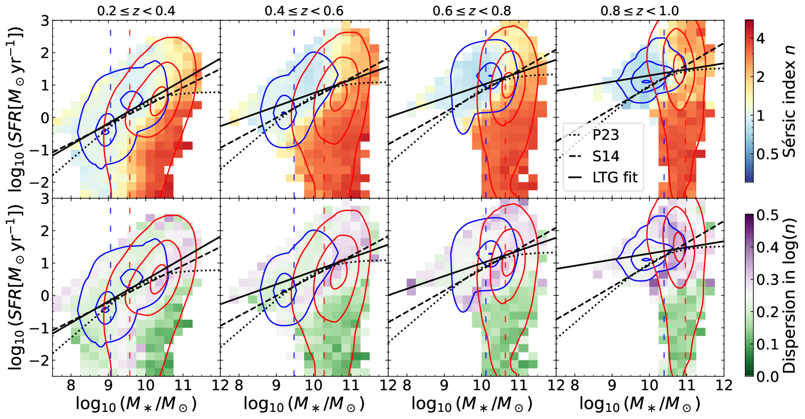
Figure 14: SFR versus $M_{\ast}$ diagrams for the four consecutive intervals of redshift, colour-coded by the median $n$ (top row) and associated dispersion around it (bottom row) in each cell of the plane. We over-plotted density contours at the 10%, 50%, and 90% levels, as well as the 90% mass completeness limit for the ETG and LTG samples (red and blue vertical dashed lines, respectively). The SFMS from Speagle et al. (2014) and Popesso et al. (2023) are displayed as black dashed and dotted lines, respectively, whereas a fit to the $M_{\ast}$–SFR relation of our sample of LTG galaxies is shown as a black solid line.

We explore how the change in the power-law exponent of the $M_{\ast}$–$R_{\mathrm{e}}$ relation varies with $n$ for Q1 galaxies. Figure 13 shows this relation for all galaxies up to $I_{\scriptscriptstyle\rm E}<23$ in the previously studied redshift bins. The colour-maps indicate the median $n$ and dispersion around it, for the top and bottom plots respectively, in each cell of the $M_{\ast}$–$R_{\mathrm{e}}$ plane, whereas the contours indicate the distributions of the LTG and ETG samples defined in Fig. 11, at the 10%, 50%, and 90% levels. Cells outside the largest of the series of contours correspond to much lower statistics at the tails of distributions. Power-law fits were performed for the $M_{\ast}$–$R_{\mathrm{e}}$ relation on both subsamples, shown as solid-red and dotted-blue lines, respectively (for galaxies with $M_{\ast}>90$% completeness limit at a given $z$). All fits are performed on at least 10 000 galaxies but due to the mass completeness limit, they were made on a restricted mass interval, which limits their quality. These fits allow us to see that at all redshifts considered, the $M_{\ast}$–$R_{\mathrm{e}}$ relation displays a much steeper slope for the ETG sample than for the LTG one, with consecutive values in each $z$-bin of $\alpha$ of 0.48, 0.66, 0.64, and 0.63 for ETG against 0.22, 0.21, 0.28, and 0.25 for LTG. Furthermore, our sample traces the dramatic increase (by a factor of 1.5) in the characteristic size of ETGs from $z\sim 0.9$ to $z\sim 0.3$, with fitted values of $R_{0}$ of 3.6 and 5.2 kpc, respectively (see Eq. 5). The fits are extended below the mass limits of each subsample (where we displayed them with dotted lines), showing agreement with the corresponding incomplete data for ETG and LTG in all redshifts intervals. Therefore the bias due to the mass limit completeness remains limited enough to reassert that, in agreement with many of the previous studies introduced above, these two galaxy populations are characterised by different $M_{\ast}$–$R_{\mathrm{e}}$ relations, hence suggesting different regimes of stellar mass assembly. However, these limitations prevent us from investigating variations in these relations across the full redshift range.

In the bottom panels of Fig. 13, the low dispersions seen in the $M_{\ast}$–$R_{\mathrm{e}}$ cells dominated by either the LTG and ETG samples confirm that the dichotomy between these two populations can be observed in the $M_{\ast}$–$R_{\mathrm{e}}$ plane as well. The highest values of dispersions are seen on the cells where LTG and ETG distributions overlap (using their contours from Fig. 13): these corresponds to the transition regions where galaxies transform from the former to the latter, hence a wide range of $n$ are observed there.

7.4 Morphology in the stellar mass–SFR plane

There is also a well-known relation between $M_{\ast}$ and SFR, usually referred to as the star-forming main sequence (SFMS; Santini et al. 2017; Rodighiero et al. 2014; Sparre et al. 2015; Cano-D´ıaz et al. 2016; Donnari et al. 2019; Muzzin et al. 2013), where the SFR is approximately proportional to the $M_{\ast}$ of the galaxy. Additionally, the relation between galaxy morphology and star-formation rate is also very strong: spiral galaxies show ongoing star-formation, while the majority of elliptical galaxies are quenched, falling below the SFMS in the $M_{\ast}$–SFR plane (e.g., Pozzetti et al. 2010; Lang et al. 2014). More massive systems are usually quenched at earlier times, following the “downsizing” scenario (e.g., Pérez-González et al. 2008; Behroozi et al. 2010; Thomas et al. 2010).

We show in Fig. 14 the $M_{\ast}$–SFR plane colour-coded by the median $n$ and its scatter in the four redshift bins. Over-plotted are the distinct mass limits at each redshift (vertical dashed lines) for the ETG and LTG galaxies. At intermediate masses ($\sim 10^{10}M_{\odot}$), there is a mix of the two populations, but some of the ETGs may be missing, due to their higher mass completeness limit. We find a good agreement between our fit to LTG galaxies (solid black line) and the relations of either Speagle et al. (2014, dashed line) or Popesso et al. (2023, dotted line) for $z=0.2-0.4$. But for higher redshifts, the mass completeness limits of our sample are such that we do not probe the low-mass part of the SFMS, leading to a very narrow mass interval, which in turns flattens the fit. However, the SFMS from previous studies still goes convincingly through the bulk of our LTG sample. The difference between a selection of LTGs versus ETGs, and star-forming versus quiescent galaxies, as well as different methods to compute stellar masses and SFRs can lead to the observed small differences. A more thorough investigation of the SFMS using Euclid Q1 data products, and additional IRAC bands, is performed in Euclid Collaboration: Enia et al. (2025). Using a deeper sample ($H_{\scriptscriptstyle\rm E}<24$) than in the current study, hence less affected by selection effects, the authors confirm that their SFMS from Euclid data agrees with the previously published results (e.g. Popesso et al. 2023) at all redshifts from 0.2 to 3.0.

Fig. 14 shows that the median $n$ values of the galaxies located in the SFMS are around 1 (corresponding to disc-like LTGs) while larger $n$ values around 4 dominate the massive, quenched distribution. This is in agreement with the trend observed for galaxies in the $0.5<z<2.5$ interval by Wuyts et al. (2011) using HST imaging, and by Martorano et al. (2025) using both HST and JWST imaging. It is worth noting that most of the $\operatorname{log_{10}}(M_{\ast}/M_{\odot})\lesssim 9.5$ galaxies below the SFMS also show low $n$ values ($n\sim 1$). We note, however, that the fraction of such objects is small (only 3.8% of galaxies in $0.2\leq z<0.4$ have $\operatorname{log_{10}}(M_{\ast}/M_{\odot})\lesssim 9.5$ and $\operatorname{log_{10}}($SFR$[M_{\odot}.\rm{yr}^{-1}])<1.5$) and is affected by incompleteness. Due to the higher mass completeness limit for the ETG sample, these objects are more likely to be missed at $\operatorname{log_{10}}(M_{\ast}/M_{\odot})\lesssim 9.5$, which biases the median $n$ towards lower values. Moreover, resolution issues could affect the $n$ estimates at faint magnitudes (see Fig. 7). Modulo these selection effects, this trend may also suggest that the quenching of the low-mass galaxy population is not so strongly coupled with morphological transformations. Regarding the associated dispersion around the median shown in Fig. 14 bottom plots, the same observation as for Fig. 13 can be made with the highest dispersion values found for the transition region in between LTG and ETG, whereas cells dominated by only one of these populations show comparatively low dispersion.

Dimauro et al. (2022) found that the drop-out of the Main Sequence was occurring for galaxies with $B/T\sim 0.2$, demonstrating that quenching was concomitant with morphological transformations, more specifically with the emergence of a prominent bulge (see also Lang et al. 2014; Bluck et al. 2014, 2022; Quilley & de Lapparent 2022). Even though $n$ is not as valuable a morphological indicator as the $B/T$ (Q25a), we do observe an increase of $n$ as galaxies drop below the SFMS.

However, we also notice in Fig. 14 that this increase of $n$ partly occurs for massive galaxies along the SFMS, with an increase from a median $n$ of 1 below $\operatorname{log_{10}}(M_{\ast}/M_{\odot})\sim 10.5$ to a median of $n=2$ above it. From the bottom panels of Fig. 14, we note however that the increased dispersion at the massive end of the SFMS indicates a mix of morphologies. This could be interpreted as morphological transformations starting prior to the shutdown of star-formation. The intermediate median $n$ ($\sim 2$) are typical of early spirals or lenticular galaxies with both bulge and disc. This would be in agreement with scenarios in which the growth of the bulge triggers the quenching of galaxies, either by morphological quenching (Martig et al. 2009) or AGN feedback (Bluck et al. 2022; Brownson et al. 2022, see e.g.). We note however that the full morphological transition from $n=1$ to $n=4$ is only completed by quenched systems below the SFMS, so we remain careful in our interpretation and do not conclude that morphological transformations occur prior to quenching, but seem to only start before it. Single-Sérsic models are not tailored to fit galaxies with both a bulge and a disc, and are prone to entirely leaving out low flux bulges, as seen in Fig. 5 bottom-left panel. As a result, they do not allow us to trace the full evolution of galaxy properties along the Hubble sequence, characterised by bulge growth (Quilley & de Lapparent 2022), so the transition from late and intermediate to early spirals (and/or lenticular) requires further investigation.

8 Summary and Perspectives

In this study, we here presented the results of Sérsic fits available within the MER catalogue (Euclid Collaboration: Romelli et al. 2025), as part of the Q1 data release of Euclid. Fits were done using two sets of structural parameters, one for the VIS image and another for the three NISP images altogether.We explore the distribution of the parameters derived at different magnitude limits, mainly up to $I_{\scriptscriptstyle\rm E}$ $\leq 23$, which is the limit recommended by the EMC to ensure reliable single-Sérsic fits (Euclid Collaboration: Bretonnière et al. 2023).

In Sect. 5, we provided an extensive series of comparison between the Sérsic parameters and other morphological measurements. We obtained a convincing consistency between them and all the other morphological products of the MER pipeline: isophotal and Sérsic parameters are well correlated and sources showing concerning differences are identified as spurious, hence helping to further clean the sample (Sect. 5.1); $n$ is correlated to the non-parametric Concentration measure, as expected (Sect. 5.2); and distribution of Sérsic parameters vary with the morphological properties predicted by Zoobot in a physically meaningful manner (Sect. 5.3). Furthermore, there is overall agreement between the Euclid Sérsic fits and those from an HST-based analysis, namely Griffith et al. (2012), with small differences possibly due to different image resolution and depth.

A first investigation of galaxy colour gradients, resulting from stellar population age and metallicity gradients, as well as varying dust content, was carried out in Sect. 6 by measuring the variations of ($R_{\rm e}$) and $n$ with observing band. On the one hand, we found that $R_{\rm e,NISP}$ values are systemically lower than $R_{\rm e,VIS}$, becoming more prominent for higher $n$. However, these differences disappear by $I_{\scriptscriptstyle\rm E}$ $>21$, for which the bulge and disc components cannot be resolved. On the other hand, $n_{\rm NISP}$ values are systemically higher than $n_{\rm VIS}$, with a slight increase of this difference at fainter magnitudes, and a clear decreasing trend with $n_{\rm VIS}$. The presence of a red bulge within a bluer disc can explain both the $R_{\rm e}$ decrease and $n$ increase with redder observing bands, but more specific trends require further investigation based on bulge and disc decomposition, to properly decipher how they result from bulge and disc colours and colour gradients. In view of the steeply decreasing variations in the bulge-to-total ratios of nearby spiral galaxies from the UV to the near infrared, the absence of variations with redshift of these NISP-to-VIS ratios across the $z=0.2-1$ range and the corresponding rest-frame ranges does not exclude redshift variations. More detailed understanding requires further study.

In order to assert the key role of morphology in galaxy evolution, and to demonstrate that the Euclid Sérsic parameters enable a wide variety of science cases, we showed how the value of $n$ is connected to the physical parameters of galaxies. This was first done by showing that the colour bimodality of galaxy populations can be seen as a projection of the two-dimensional colour–$n$ bimodality, which allows to define robust LTG and ETG subsamples. These two galaxy populations display markedly different behaviours in their $M_{\ast}$–$R_{\rm e}$ relations with a steeper slope for ETG compared to LTG, indicative of different regimes of $M_{\ast}$ assembly. They also occupy different loci in the $M_{\ast}$–SFR plane, with ETG at higher masses and further down below the Main Sequence of star-forming galaxies, indicating that morphological transformations occur in parallel to the quenching of galaxies.

The implementation of Sérsic fits within the Euclid processing function ensures that Sérsic parameters will be available for all galaxies observed by Euclid over its years of operation. Therefore, Euclid is progressively building the largest morphological catalogue available, with an estimated total number of 450 000 000 galaxies with $I_{\scriptscriptstyle\rm E}$ $<23$ reliably fitted by the end of the mission. With this first study of Sérsic parameters on the Q1 area we demonstrate the quality, robustness, and usefulness of these data to study galaxy evolution, paving the way to many more analysis that will benefit from leveraging these informations. The EWS and EDS will enable the study of morphological transformations across the large-scale structures and over cosmic times. However, due to the limitations of a single-component model that we highlighted here, and which are more extensively discussed in Q25a, further work remains to be done to characterise in-depth the morphology of galaxies.

One pressing issue, and a direct follow-up of Sérsic fits, is to perform reliable bulge and disc decomposition on galaxies from Q1. This would allow one to investigate the history of galaxy morphology beyond the ETG/LTG dichotomy and hopefully to trace how galaxies evolved and transformed to build up the present-day Hubble sequence. Such an analysis would also raise new challenges in terms of methodology, to account for varying selection effects for different morphological types or differential chromatic effects affecting bulges and discs (Papaderos et al. 2023). Additionally, more complex models could also be built for accordingly more specific studies, e.g., the addition of bars to study the barred galaxies identified in Euclid (Euclid Collaboration: Huertas-Company et al. 2025), or of point-sources to account for AGN contribution.

Appendix A Comparison of model photometry with isophotal and adaptive aperture magnitudes

When fitting Sérsic profiles, a model magnitude is computed for each fitted galaxy, which can be compared with other methods to determine photometry. Figure 15 shows the difference between the model photometry $m_{\rm model}$ computed in the $I_{\scriptscriptstyle\rm E}$ band and both the isophotal magnitude $m_{\rm iso}$ (corresponding to FLUX$\_$SEGMENTATION in the MER catalogue) and the adaptive aperture photometry within 2.5 times the Kron radius $m_{\rm auto}$ (corresponding to FLUX$\_$DETECTION$\_$TOTAL in the MER catalogue), as a function of either magnitude and as a function of the $n$ measured in the $I_{\scriptscriptstyle\rm E}$ band, in the top and bottom panels respectively. Median differences in bins of either magnitude or $n$ are displayed as red points, and the errorbars indicate $\pm 1\sigma$ ($\sigma$ being the 0.68 quantile of the absolute differences to the median). The top-left panel shows the difference between the model and isophotal magnitudes, whose median value is 0.00 in the two brightest magnitude intervals, which then continuously decreases to $-0.13$ in the faintest magnitude interval. All differences for $I_{\scriptscriptstyle\rm E}$ $<23$ are below 1$\sigma$. The dispersion is very stable, with values between 0.07 and 0.10 across the seven magnitudes of $m_{\rm iso}$, and between 0.07 and 0.08 for $I_{\scriptscriptstyle\rm E}$ $<23$. The number of outliers with large differences increase with fainter magnitudes as a result of the increasing number of sources and decreasing signal-to-noise ratio. The top-right panel shows the difference between the model and adaptive aperture photometry, whose medians are all positive, with values ranging from 0.05 to 0.09, hence of the same order as the median differences between model and isophotal magnitudes. All median differences are below the 1$\sigma$ level with again a very stable dispersion between 0.07 and 0.10.

For both magnitude differences, the bottom panels of Fig. 15 indicate that while there is no magnitude effect, there is a morphological trend of differences decreasing with $n$. The median differences between model and isophotal magnitudes start at zero for the lowest values of $n$ and decreases continuously to reach $-0.15$ for $n>4$. The median differences between model and adaptive aperture magnitudes follow a very similar decrease, but with an offset, since values decrease from $0.14$ to $-0.01$ for the lowest to highest bins of $n$. The black diamond symbols and solid line in both plots show the difference computed mathematically for a pure circular Sérsic profile between its total magnitude and the adaptive aperture magnitude computed within 2.5 times the Kron radius, which only depends on $n$ (taken from Graham & Driver 2005). Because the fitted galaxies are not perfectly approximated by Sérsic profiles, we would expect the difference between the model and adaptative aperture photometry to follow this theoretical behaviour, with some dispersion around it. However, we observe that this prediction matches instead the median difference between isophotal and model magnitudes. The behaviour of decreasing median differences for higher $n$ remains for the difference between the model and adaptative aperture photometry, but with a 0.15 magnitude offset.

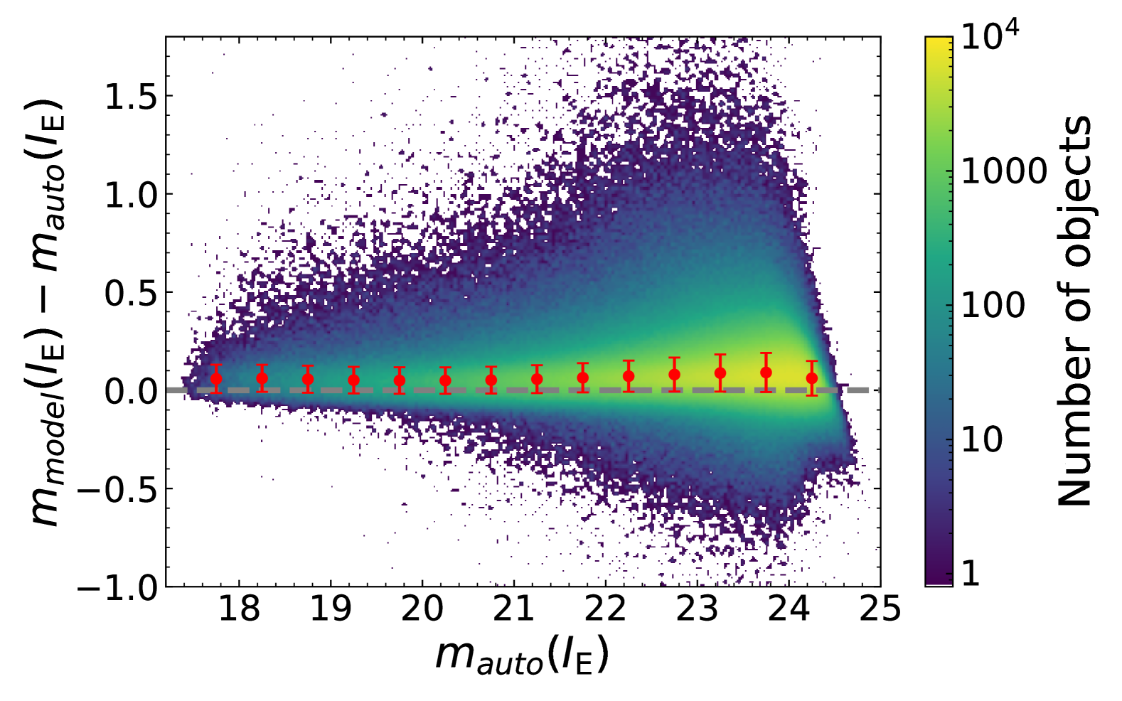
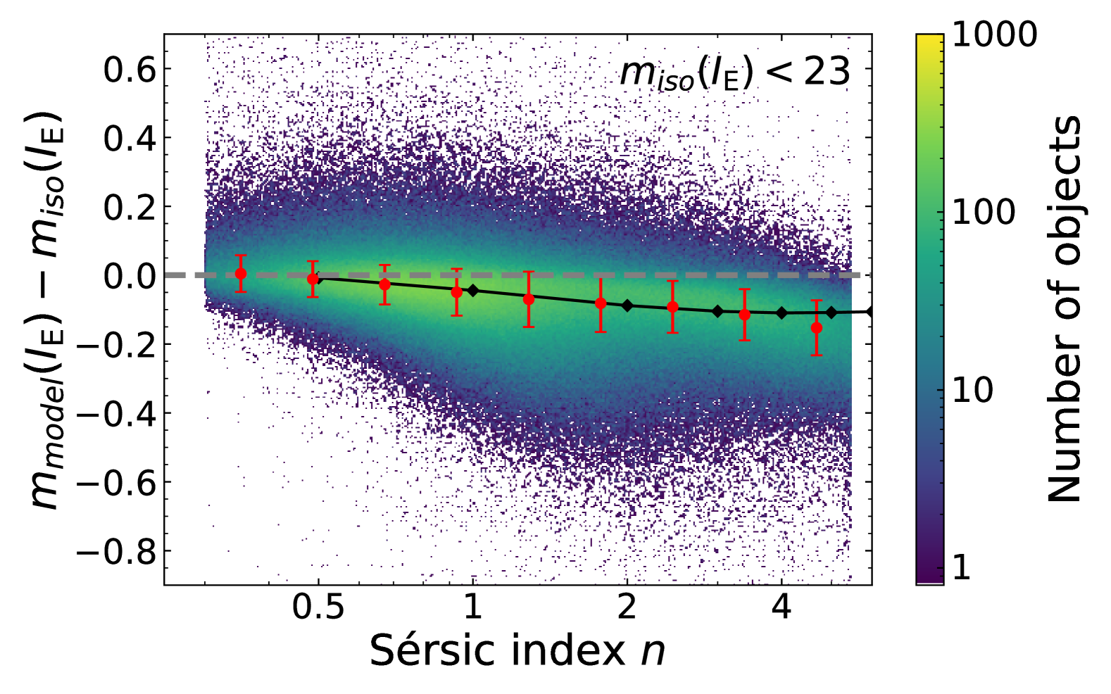
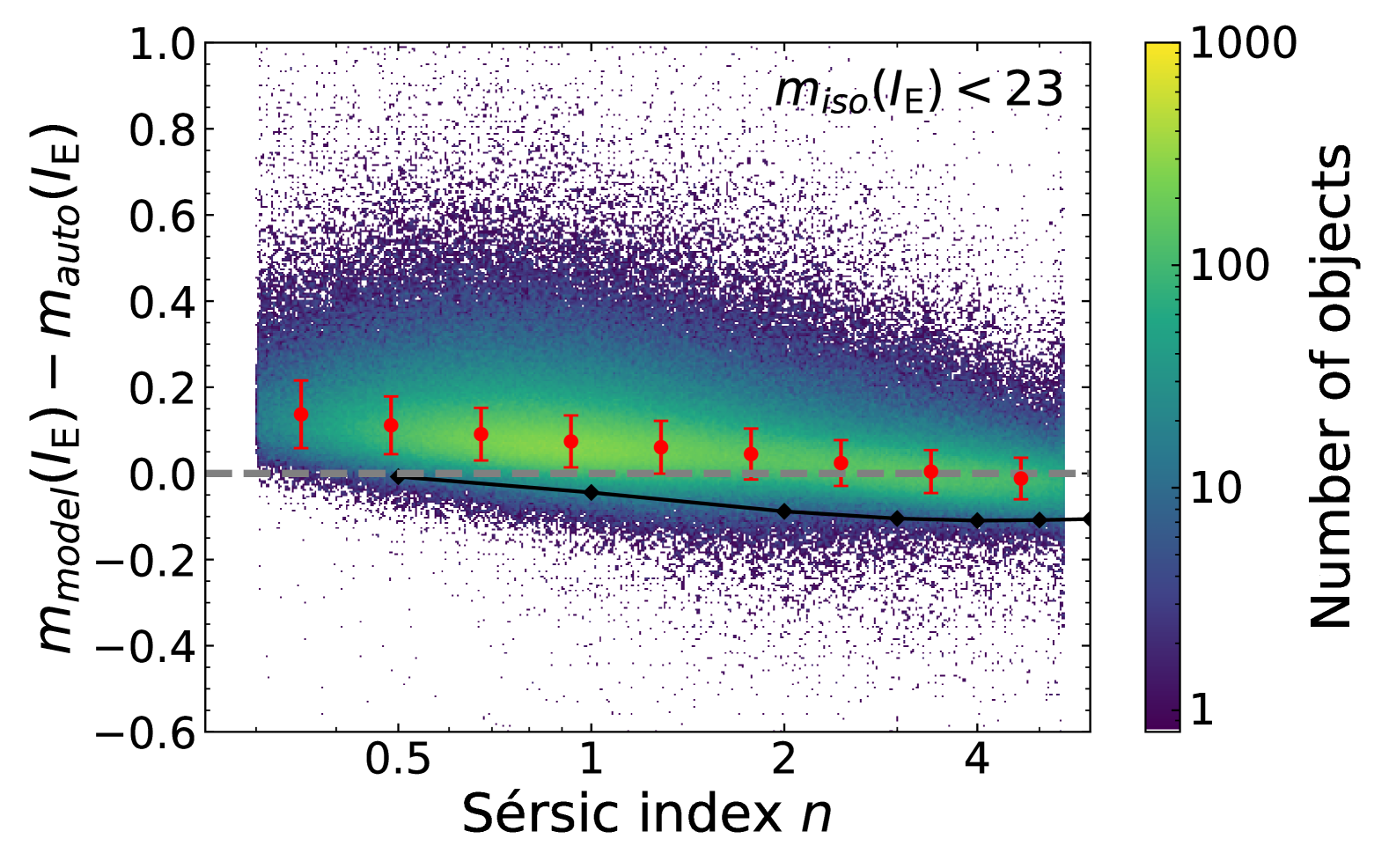
Figure 15: Difference between the isophotal $m_{\rm iso}$ and model magnitude $m_{\rm model}$ (left) and between the adaptive aperture $m_{\rm auto}$ and model magnitude (right), as a function of either the magnitude compared to model photometry (top), or $n$ (bottom). Red points and error bars indicate median differences and associated dispersion around them. The black line indicates the mathematical prediction of $m_{\rm model}-m_{\rm auto}$ for a pure Sérsic profile, and unexpectedly matches the values of $m_{\rm model}-m_{\rm iso}$ whereas it is shifted by 0.15 mag below the measured $m_{\rm model}-m_{\rm auto}$ that it aims at predicting.

Appendix B Colour–Stellar mass–Sérsic index  space

We show in Fig. 16 the $(u-r)$ colour versus $M_{\ast}$, colour-coded with the median $n$ as in Figs. 13 and 14. This allows us to see that the colour–$n$ bimodality can also be extended as a 3-dimensional colour–$M_{\ast}$–$n$ bimodality, with red galaxies having steeper profiles being more massive than their bluer counterparts. The top row shows the density contours at the 10%, 50%, and 90% levels for the ETG and LTG subsamples defined in Sect. 7.1, whereas the bottom row uses a cut at $n_{\rm lim}=2.5$ in order to divide the sample into two new classes. This leads to a more spread out distribution of the two new subsamples, with significant overlaps at all redshifts. This illustrates that it is preferable to not use $n$ alone to separate galaxy populations but rather use joint conditions, such as colour or stellar mass. We checked that using a different criterion on $n$ only, such as using a different $n_{\rm lim}$ or two limits, i.e., having $n\leq n_{1}$ and $n\geq n_{2}$ with $n_{1}<n_{2}$, leads to similar results as shown in Fig. 16 with $n_{\rm lim}=2.5$. The suggested selection of Eq. (4), or a similar method adapting the presented process to the available data, therefore allows to highlight more significantly the different behaviours of early and late galaxies.

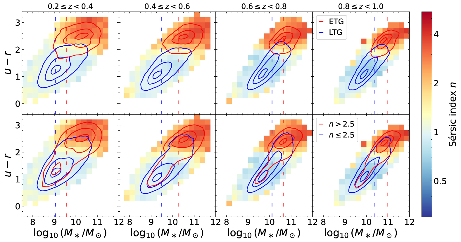
Figure 16: Redshift evolution of $M_{\ast}$ versus ($u-r$) colour, colour-coded by the median $n$ in each cell. In the top row, we over-plotted density contours at the 10%, 50%, and 90% levels, for the ETG and LTG samples, as in previous figures, whereas the bottom row the blue and red contours correspond to galaxies with $n\leq 2.5$ and $n>2.5$ respectively, displaying significant overlaps in both colour and mass. In all panels the vertical dashed lines indicate the 90% mass completeness limit of the ETG and LTG samples. The colour–concentration bimodality evidenced in Fig. 11 of Sect. 11 is also present in the $M_{\ast}$ –colour plane.