Fine-Grained Complexity of Computing Degree-Constrained Spanning Trees

Abstract

We investigate the computation of minimum-cost spanning trees satisfying prescribed vertex degree constraints: Given a graph $G$ and a constraint function $D$, we ask for a (minimum-cost) spanning tree $T$ such that for each vertex $v$, $T$ achieves a degree specified by $D(v)$. Specifically, we consider three kinds of constraint functions ordered by their generality—$D$ may either assign each vertex to a list of admissible degrees, an upper bound on the degrees, or a specific degree. Using a combination of novel techniques and state-of-the-art machinery, we obtain an almost-complete overview of the fine-grained complexity of these problems taking into account the most classical graph parameters of the input graph $G$. In particular, we present SETH-tight upper and lower bounds for these problems when parameterized by the pathwidth and cutwidth, an ETH-tight algorithm parameterized by the cliquewidth, and a nearly SETH-tight algorithm parameterized by treewidth.

1 Introduction

Algorithms for computing minimum-cost spanning trees of graphs are, in many ways, cornerstones of computer science: classical results such as the algorithms of Prim or Kruskal are often among the first graph algorithms presented to undergraduate students. And yet, in many situations it is necessary to compute not only a spanning tree, but one that satisfies additional constraints. In this article, we investigate the computation of (minimum-cost) spanning trees which satisfy prescribed constraints on the degrees of the graph’s vertices.

More precisely, given an edge-weighted graph $G$ and a constraint function $D\colon V(G)\rightarrow\circ$, our aim is to determine whether there is a spanning tree $T$ of $G$ such that for each $v\in V(G)$, $\mathrm{deg}_{T}(v)\in D(v)$—and if the answer is positive, output one of minimum cost. Depending on the form of the constraint function, we distinguish between the following three computational problems:

1. in Set of Degrees Minimum Spanning Tree (MST), $D$ maps each vertex to a set of positive integers;

2. in Bounded Degree MST, the images of $D$ are all sets of consecutive integers starting from $1$; and

3. in Specified Degree MST, the images of $D$ are singletons.

While the above problems are in fact ordered from most to least general, the considered types of constraints can each be seen as natural and fundamental in its own right. Indeed, Bounded Degree MST characterizes a crucial base case in the Thin Tree Conjecture [20, 27] and has been extensively studied in the approximation setting where one is allowed to violate the constraints by an additive constant [15, 21, 33]. At the same time, Specified Degree MST and Set of Degrees MST form natural counterparts to the classical $f$-Factor and General $f$-Factor problems [35, 7, 16, 17], respectively. The -hard connected variants of the latter two problems have been studied in the literature as well [11, 6, 18].

While classical minimum-cost spanning trees can be computed on general graphs in almost linear time [3, 4], we cannot hope to achieve such an outcome for even the easiest of the three problems considered here—indeed, Specified Degree MST is -hard as it admits a straightforward reduction from Hamiltonian Path. Naturally, this only rules out efficient algorithms on general graphs; in reality, the actual running time bounds will necessarily depend on the structural properties of the input graphs—for instance, all three degree-constrained MST problems admit trivial linear-time algorithms on trees. In this article, we investigate the fine-grained running time bounds for solving these problems taking into account the structure of the input graphs and obtain a surprisingly tight classification under the Exponential Time Hypothesis (ETH) [24] along with its strong variant (SETH) [23].

Contributions. We are not the first to investigate tight running time bounds for constrained variants of the (Minimum) Spanning Tree problem. For instance, Cygan, Nederlof, Pilipczuk, Pilipczuk, van Rooij and Wojtaszczyk [9] obtained an essentially tight $\mathcal{O}^{*}(4^{\operatorname{tw}(G)})$ bound for computing (not necessarily minimum) spanning trees with a specified number of leaves, where $\operatorname{tw}(G)$ is the treewidth of the input graph and $\mathcal{O}^{*}$ suppresses constant as well as polynomial factors of the input. In particular, their results include a randomized algorithm which solves that problem in the specified time, as well as a lower bound based on SETH which rules out any improvements to the base of the exponent even if treewidth is replaced by the larger parameter pathwidth ($\operatorname{pw}(G)$).

Unfortunately, this result—or any other known results on computing constrained spanning trees (see, e.g., [37])—does not translate into the degree-constrained setting considered here. In fact, as our first contribution (Theorem 6.15) we rule out an algorithm with this running time by establishing a SETH-based lower bound that essentially excludes any algorithm solving Specified Degree MST (the easiest of the three problems considered here) in time faster than $\mathcal{O}^{*}((2r)^{\operatorname{pw}(G)})$, where $r$ is the maximum degree requirement in the image of $D$, even if $G$ is edge-unweighted. We complement the lower bound with a tight algorithmic upper bound that holds for the most general of the three kinds of degree constraints. In particular, we obtain a randomized algorithm solving Set of Degrees MST in time $\mathcal{O}^{*}((2r)^{\operatorname{pw}(G)})$ (Theorem 6.1) and show that this algorithm can also be translated to treewidth, albeit with an “almost optimal” running time of $\mathcal{O}^{*}((2r+2)^{\operatorname{tw}(G)})$ (Theorem 5.1).

The above results raise the question of whether one can also solve these problems on more general inputs, notably unweighted dense graphs. More concretely, can we efficiently compute degree-constrained spanning trees by exploiting the classical graph parameter clique-width ($\operatorname{cw}$)? As our next contribution, in Theorem 3.1 we obtain a highly non-trivial $n^{\mathcal{O}(\operatorname{cw})}$ algorithm solving Set of Degrees MST on $n$-vertex graphs—a result which is tight under the ETH [13] and generalizes the known algorithm for Hamiltonian Path under the same parameterization [1].

Under current complexity assumptions, neither Theorem˜6.1 nor Theorem˜3.1 can be improved to yield fixed-parameter algorithms for our problems of interest under the considered structural parameterizations. However, the question still remains whether one can obtain (tight) fixed-parameter algorithms under different, more restrictive parameterizations. As our third and final set of contributions, we obtain tight “fixed-parameter” running time bounds with respect to the graph parameter cutwidth $\operatorname{ctw}$ [5, 34]. In particular, we design a randomized algorithm solving Set of Degrees MST in time $\mathcal{O}^{*}(3^{\operatorname{ctw}(G)})$ (Theorem 7.1) and a complementary SETH-based lower bound which excludes running times of the form, e.g., $\mathcal{O}^{*}(2.999^{\operatorname{ctw}(G)})$, even for Specified Degree MST in the edge-unweighted case (Theorem 7.8). A summary of our results is provided in Table 1.

Parameter	Specified Degree MST	Set of Degrees MST
	Lower bound	Upper bound
Clique-width	$n^{o(k)}$ [13]	$n^{\mathcal{O}(k)}$ (Thm. 3.1)
Treewidth	$\mathcal{O}^{*}\big{(}(2r-\varepsilon)^{k}\big{)}$ (Thm. 6.15)	$\mathcal{O}^{*}\big{(}(2r+2)^{k}\big{)}$ (Thm. 5.1)
Pathwidth	$\mathcal{O}^{*}\big{(}(2r-\varepsilon)^{k}\big{)}$ (Thm. 6.15)	$\mathcal{O}^{*}\big{(}(2r)^{k}\big{)}$ (Thm. 6.1)
Cutwidth	$\mathcal{O}^{*}\big{(}(3-\varepsilon)^{k}\big{)}$ (Thm. 7.8)	$\mathcal{O}^{*}\big{(}3^{k}\big{)}$ (Thm. 7.1)

Table 1: Overview of our results. Here, $k$ always denotes the respective graph parameter, $r$ is the maximum degree requirement in the image of $D$ and $n$ is the order of the input graph. All lower bounds and the clique-width algorithm are obtained for the edge-unweighted variants. All obtained lower and upper bounds directly transfer to the remaining (more or less general) problems.

Paper Organization. After introducing the necessary preliminaries in Section 2, we begin our exposition by presenting our algorithm for dense graph parameters in Section 3. Next, in Section 4 we introduce the machinery that will be employed for the remaining upper bounds, including Cut&Count, the Isolation Lemma and our problem-specific modifications thereof. We then proceed with the algorithms and lower bounds for treewidth (Section 5), pathwidth (Section 6) and cutwidth (Section 7).

Proof Techniques. To obtain our algorithm for Set of Degrees MST on unweighted graphs parameterized by clique-width, our high-level aim is to employ the typical leaf-to-root dynamic programming approach that is used in almost all applications of decompositional graph parameters. There, one intuitively seeks to identify and maintain a correspondence between a suitably defined notion of “partial solution” in the graph constructed so far, and a (typically combinatorial and compact) representation of that partial solution that is stored as an entry in our records. However, attempting to follow this approach directly for Set of Degrees MST on clique-width decompositions fails, as the number of natural “representations” of partial solutions is not bounded by $n^{f(\operatorname{cw})}$ (for any $f$). In order to circumvent this issue and obtain the sought-after single-exponential  algorithm, we will “decompose” these initial representations into collections of more concise representations for partial solutions. Crucially, this step breaks the one-to-one correspondence between individual entries we will store in our records and individual partial solutions in the graph constructed so far; instead, all we will maintain is that no matter what operations happen later, our records will be sufficient to either correctly reject or accept.

Concretely, to do this we show that each natural representation $R$ of a partial solution at some partially processed graph $H$ which is not already “well-structured” can be reduced into two new representations $R_{1}$, $R_{2}$, each of which contains slightly more “structure” than $R$. Crucially, both $R_{1}$ and $R_{2}$ are weaker than $R$ in the sense that each valid extension (to a full solution) of either of $R_{1}$, $R_{2}$ is also a valid extension for $R$—and we prove that $R_{1}$ and $R_{2}$ together are exactly as strong as $R$. Intuitively, $R$ behaves as an “OR” of $R_{1}$ and $R_{2}$ in the sense of extensibility. Apart from actually proving the safeness of this representation reduction rule, another difficulty lies in the fact that it is not a-priori clear how to exhaustively apply the rule within the desired runtime bound. Nevertheless, by carefully selecting the order of reductions, we can efficiently obtain a bounded-size family of “maximally-structured” representations that are, as a whole, equivalent to the set of initial representations of $H$.

To implement this approach, it is useful to avoid working with clique-decompositions directly, but rather to use the closely related notion of NLC-width and NLC-decompositions. This is without loss of generality, as NLC-width is known to differ from clique-width by at most a factor of $2$. The advantage of NLC-width here is that it avoids adding edges into the graph processed so far, which is important for dealing with the opaque representations we need to use for the algorithm.

To obtain algorithms for pathwidth, treewidth and cutwidth we achieve our tight algorithmic upper bounds using the Cut&Count technique that has been pioneered precisely to obtain tight bounds for connectivity problems [9]. Unfortunately, a direct application of that technique would not be able to break the $(2r+2)^{k}$ barrier even for pathwidth. Here, we achieve a further improvement by introducing a novel “lazy coloring” step to obtain SETH-tight bounds for pathwidth and cutwidth; for the latter, we need to combine our new approach with the AM/GM inequality technique [25]. While we cannot achieve the same improvement for treewidth, obtaining the current $(2r+2)^{k}$ bound instead required the use of multidimensional fast Fourier transformations [36].

Finally, for our tight SETH-based lower bounds, on a high level we follow the approach of Lokshtanov et al. [31]—but with a twist. In particular, it is not at all obvious how to obtain a classical “one-to-one” reduction to several of our problems, and this issue seems difficult to overcome with standard gadgets. Intuitively, for Bounded and Specified Degree MST a small separator in the graph prevents the existence of partial solutions on one side with strongly varying requirements. To circumvent this issue, we employ Turing reductions instead of the usual one-to-one reductions used for SETH; to the best of our knowledge, this is the first time such reductions are used for structural parameters. Moreover, in the specific case of cutwidth, our reduction also exhibits a highly non-standard behavior: instead of producing graphs with cutwidth $n+\delta$ where $n$ is the input complexity measure and $\delta$ some fixed constant, we can only obtain graphs with cutwidth $\omega\cdot n+\delta$, where $\omega>1$. Under normal circumstances, this would not allow us to obtain a tight bound under SETH; however, here we construct a family of reductions that allows us to set $\omega$ arbitrarily close to $1$ and show that this still suffices to achieve the desired bound.

2 Preliminaries

We assume basic familiarity with graph terminology [10], the Exponential Time Hypothesis (ETH) along with its strong variant (SETH) [24, 23] and the $\mathcal{O}^{*}$ notation which suppresses polynomial factors of the input size. For a positive integer $k$, we use $[k]$ to denote the set $\{1,\dots,k\}$ and $[k]_{0}$ the set $\{0,1,\dots,k\}$. We denote the unit vector of the $i$’th dimension with $\mathbf{e}_{i}$ and the zero vector with $\mathbf{0}$.

For a function $g:U\rightarrow V$, that is not explicitly defined as a weight function, and for a set $C\subseteq U$, we denote by $g(C)$ the set $\{g(x)\colon x\in C\}$. If $g$ is explicitly defined as a weight function, where $V$ is some ring, we denote by $g(C)$ the sum $\sum_{x\in C}g(x)$.

Let $G=(V,E)$ be a graph. For a set of edges $F\subset E$, we denote by $G[F]$ the graph $(V^{\prime},F)$, where $V^{\prime}$ is the set of endpoints of $F$. For a subgraph $H$ of $G$ and a vertex $v$ of $G$, we denote by $\mathrm{deg}_{H}(v)$ the degree of $v$ in $H$. For convenience, when $H=G[F]$ for a set of edges $F$, we use $\mathrm{deg}_{F}(v)$ for $\mathrm{deg}_{G[F]}(v)$. We denote by $\cc(G)$ the set of all connected components of $G$ and by $N_{G}(v)$ the neighborhood of $v$ in $G$. Let $S$ be a totally ordered set. Given a mapping $f:U\rightarrow\mathbb{Z}$ we define the family $\big{(}\leq f(u)\big{)}_{u\in S}$ as the family of all vectors $v\in\mathbb{Z}^{S}$ where $0\leq v_{u}\leq f(u)$ for all $u\in S$. For a mapping $f:U\rightarrow V$ and a set $S\subseteq U$, we define the restriction $f|_{S}:S\rightarrow V$ as the restriction of $f$ to $S$. For some element $u$ (not necessarily in $U$), and a value $v\in V$, we define the mapping $f[u\mapsto v]:U\cup\{u\}\rightarrow V$ as the mapping

$$f[u\mapsto v](u^{\prime})=\begin{cases}v&\colon\text{if }u^{\prime}=u,\\ f(u^{\prime})&\colon\text{otherwise}.\end{cases}$$

We denote multisets using angle brackets. We say $a=b$ when two elements $a$ and $b$ have the same value, and $a\mathrel{\mathchoice{\ooalign{\raisebox{-1.10063pt}{$\displaystyle\widehat{}$}\cr\hbox{\set@color$\displaystyle=$}\cr}}{\ooalign{\raisebox{-1.10063pt}{$\textstyle\widehat{}$}\cr\hbox{\set@color$\textstyle=$}\cr}}{\ooalign{\raisebox{-0.77043pt}{$\scriptstyle\widehat{}$}\cr\hbox{\set@color$\scriptstyle=$}\cr}}{\ooalign{\raisebox{-0.55031pt}{$\scriptscriptstyle\widehat{}$}\cr\hbox{\set@color$\scriptscriptstyle=$}\cr}}}b$ when $a$ and $b$ refer to the same object. For example, suppose we have a multiset $\langle a,b\rangle$, where $a=3$ and $b=3$. Then $a=b$ but $a\not\mathrel{\mathchoice{\ooalign{\raisebox{-1.10063pt}{$\displaystyle\widehat{}$}\cr\hbox{\set@color$\displaystyle=$}\cr}}{\ooalign{\raisebox{-1.10063pt}{$\textstyle\widehat{}$}\cr\hbox{\set@color$\textstyle=$}\cr}}{\ooalign{\raisebox{-0.77043pt}{$\scriptstyle\widehat{}$}\cr\hbox{\set@color$\scriptstyle=$}\cr}}{\ooalign{\raisebox{-0.55031pt}{$\scriptscriptstyle\widehat{}$}\cr\hbox{\set@color$\scriptscriptstyle=$}\cr}}}b$. In this case, we also say that $a$ and $b$ are distinct.

Problem Definitions.

We formally define our problems of interest below:

(Weighted) Set of Degrees MST Input: Graph $G=(V,E)$, edge weight $w:E\to\mathbb{R}_{\geq 0}$, function $D:V(G)\rightarrow 2^{\mathbb{N}}$, bound $B\in\mathbb{R}_{\geq 0}$ Question: Does $G$ admit a spanning tree $T$ of cost at most $B$ such that $\mathrm{deg}_{T}(v)\in D(v)$ for each $v\in V(G)$?

Bounded Degree MST and Specified Degree MST are defined analogously, but there the images of $D$ are sets of the form $[i]$ or $\{i\}$ (for some integer $i$), respectively. We use $r$ to denote $\max_{v\in V(G),x\in D(v)}x$.

For the unweighted versions of the problems above, we omit the edge weights $w$ and the cost bound $B$ from the input and hence instances merely consist of a pair $(G,D)$. The unweighted versions of all three considered problems are -hard as they admit a straightforward reduction from Hamiltonian Path. Moreover, there are trivial weight- and graph-preserving reductions from (weighted) Bounded Degree MST to (weighted) Set of Degrees MST and from (weighted) Specified Degree MST to (weighted) Bounded Degree MST. For the latter, every instance of Specified Degree MST not satisfying $\sum_{v\in V(G)}d(v)=2n-2$ can be rejected, while that which does satisfy the equality is equivalent to the same instance of Bounded Degree MST.

Structural Parameters.

We now define the graph parameters considered in this work.

Treewidth and pathwidth. A tree decomposition of a graph $G=(V,E)$ is a pair $(\mathcal{T},\mathcal{B})$ where $\mathcal{T}$ is a tree and $\mathcal{B}:V(\mathcal{T})\rightarrow 2^{V}$ assigns the nodes of $\mathcal{T}$ to subsets of $V$ such that

• for each $v\in V$ there exists $x\in V(\mathcal{T})$ with $v\in\mathcal{B}(x)$,

• for each $e\in E$ there exists $x\in V(\mathcal{T})$ with $e\subseteq\mathcal{B}(x)$,

• for each $v\in V$ the set $\{x\in V(\mathcal{T})\colon v\in\mathcal{B}(x)\}$ induces a connected subgraph of $\mathcal{T}$.

A path decomposition is a tree decomposition $(\mathcal{T},\mathcal{B})$, where $\mathcal{T}$ is a simple path. When the decomposition $(\mathcal{T},\mathcal{B})$ is clear from context, we denote $B_{v}=\mathcal{B}(v)$, and $\mathcal{V}=V(\mathcal{T})$. When the decomposition is clear from context, we will sometimes denote the decomposition by $\mathcal{T}$ and assume that $\mathcal{B}$ is implicitly given with $\mathcal{T}$.

We define the width of a tree decomposition $(\mathcal{T},\mathcal{B})$ as $\operatorname{tw}(\mathcal{T},\mathcal{B})=\max\{x\in\mathcal{V}\}|\mathcal{V}(x)|-1$. The treewidth (pathwidth) of a graph $G$, denoted by $\operatorname{tw}(G)$ ($\operatorname{pw}(G)$) is the smallest width of a tree decomposition (path decomposition) of $G$. Finally, a path decomposition can be defined by a sequence of sets $B_{1},\dots,B_{h}$, that corresponds to the path decomposition $(P_{h},\mathcal{B})$, where $P_{h}$ is a simple path over the vertices $v_{1},\dots v_{h}$, and $\mathcal{B}=\{B_{i}\colon i\in[h]\}$, where $B_{i}$ is the bag corresponding to the node $v_{i}$ for $i\in[h]$.

In the following, we define the notion of a nice tree decomposition. Different (close) notions of nice decompositions were defined in the literature, the first of which was defined by Kloks [28]. It is well-known, that given a tree (or path) decomposition of a graph $G$, one can construct a nice tree (or path, respectively) decomposition of the same width and polynomial size in $|V|$ in polynomial time [28]. Such a decomposition can be easily modified to meet our requirements in the same running time. We will use the notion of a nice tree decomposition to simplify the presentation of our algorithms.

Definition (Nice tree decomposition).

A nice tree decomposition $(\mathcal{T},\mathcal{B})$ of a graph $G=(V,E)$ is called a tree decomposition of $G$ where $\mathcal{T}$ is rooted at a node $r\in\mathcal{V}$, and it holds for each $x\in\mathcal{V}$ that $x$ has one of the following types:

• A leaf node: $x$ is a leaf of $\mathcal{T}$. It holds that $B_{x}=\emptyset$. We define $G_{x}=(V_{x},E_{x})$ as an empty graph.

• An introduce vertex node $(v\in V)$: where $x$ has a single child $x^{\prime}$ and $B_{x}=B_{x^{\prime}}\cup\{v\}$. We define $G_{x}=(V_{x},E_{x})$ as the graph obtained from $G_{x^{\prime}}$ by adding the vertex $v$ to $V_{x^{\prime}}$.

• An introduce edge node $(e\in E)$: where $x$ has a single child $x^{\prime}$ and $B_{x}=B_{x^{\prime}}$. We define $G_{x}=(V_{x},E_{x})$ as the graph obtained from $G_{x^{\prime}}$ by adding the edge $e$ to $E_{x^{\prime}}$.

• A forget vertex node $(v\in V)$: where $x$ has a single child $x^{\prime}$ and $B_{x^{\prime}}=B_{x}\cup\{v\}$. We define $G_{x}=G_{x^{\prime}}$.

• A join node: where $x$ has exactly two children $x_{1}$ and $x_{2}$, and $B_{x_{1}}=B_{x_{2}}=B_{x}$. We define $G_{x}$ the graph resulting from the disjoint union of $G_{x_{1}}$ and $G_{x_{2}}$ by identifying both copies of each vertex $v\in B_{x}$ (i.e., we consider each copy as a distinct vertex when computing the union, and after that we identify the copies).

Moreover, it holds for a nice tree decomposition that $B_{r}=\emptyset$ and for each $e\in E$ there exists exactly one node $x$ that introduces $e$. Note that $G_{r}$ is isomorphic to $G$. A nice path decomposition is a nice tree decomposition that does not have any join nodes.

NLC-Width. To present our algorithmic result for clique-width we will use a closely related graph measure called NLC-width, which we define below. A $k$-graph $G$ is a graph equipped with a vertex labeling $\texttt{lab}_{G}$ that assigns each vertex an integer from $[k]$. An initial $k$-graph $\bullet_{i}$ is a graph consisting of a single vertex labeled $i$. Given an edge mapping $\alpha\subseteq[k]^{2}$ and a relabeling function $\beta:[k]\rightarrow[k]$, we define the join operation $\oplus_{\alpha}^{\beta}$ (where we omit the superscript if $\beta$ is the identity) as follows. For two $k$-graphs $G_{1}$ and $G_{2}$, $G_{1}\oplus_{\alpha}^{\beta}G_{2}$ is the $k$-graph obtained by:

1. performing the disjoint union of $G_{1}$ and $G_{2}$, then

2. adding an edge between every vertex $v_{1}\in V(G_{1})$ and every vertex $v_{2}\in V(G_{2})$ such that $(\texttt{lab}(v_{1}),\texttt{lab}(v_{2}))\in\alpha$, and finally

3. for each $v\in V(G_{i})$, changing the label of $v$ to $\beta(\operatorname{lab}(v))$.

Naturally, join operations can be chained together, and we call an algebraic expression using initial $k$-graphs as atoms and join operations as binary operators an NLC-decomposition of the graph produced by the expression. A graph $G$ has NLC-width $k$ if $k$ is the minimum integer such that (some vertex labeling of) $G$ admits an NLC-decomposition involving at most $k$ labels. We denote by $\mathcal{T}$ the tree corresponding to the NLC-decomposition and by $\mathcal{V}=V(\mathcal{T})$ the set of all nodes of the tree. For $x\in\mathcal{V}$, we denote by $G_{x}$ the graph obtained by the algebraic expression $x$ and by $V_{x}$ the set $V(G_{x})$. For a function $f:V(G)\rightarrow\circ$, we write $f_{x}$ for $f|_{V_{x}}$.

It is well known that for every graph $G$ with NLC-width NLCw and clique-width cw, $\texttt{NLCw}\leq\texttt{cw}\leq 2\cdot\texttt{NLCw}$ [26, 2]; moreover, this relationship is constructive and so known algorithms for computing approximately-optimal decompositions for clique-width [14] also yield approximately-optimal NLC-decompositions. Intuitively, NLC-width can be seen as an analogue of clique-width where edge addition and relabeling occurs in a “single-shot fashion” rather than gradually.

Cutwidth. A linear arrangement $\ell=v_{1},\dots,v_{n}$ of a graph $G$ is a linear ordering of the vertices of $G$. Let $V_{i}=\{v_{1}\dots v_{i}\}$, and $\overline{V}_{i}=V\setminus V_{i}$. We define the cut-graph $H_{i}=G[V_{i},\overline{V}_{i}]$ as the bipartite graph induced from $G$ by the edges having exactly one endpoint in $V_{i}$. The width of a linear arrangement $\ell$ is defined by $w(\ell)=\max\{|E(H_{i})|\colon i\in[n]\}$. The cutwidth of a graph $G$ (denoted $\operatorname{ctw}(G)$) is defined as the smallest width of a linear arrangement of $G$. A linear arrangement of minimum width can be computed in time $2^{\mathcal{O}(\operatorname{ctw}(G)^{2})}\cdot n^{\mathcal{O}(1)}$ [19], and there is no single-exponential algorithm for the problem unless the ETH fails [29].

3 Dense Graph Parameters

For the remainder of this section, let $(G,D)$ be a given unweighted instance of Set of Degrees MST, where $G$ is an $n$-vertex graph of NLC-width $k$, and let us consider a given NLC-decomposition $\phi$ of $G$ using $k$ labels. In this section, all vectors are integer-valued and $k$-dimensional. For a node $x\in\mathcal{V}$, we denote $\operatorname{lab}_{x}=\operatorname{lab}_{G_{x}}$. The aim of this section is to establish the following theorem:

Theorem 3.1.

There exists an algorithm that, given an $n$-vertex instance $(G,D)$ of unweighted Set of Degrees MST together with an NLC-decomposition of $G$ using $k$ labels, solves the problem in time $n^{\mathcal{O}(k)}$.

Definitions.

Let us first define the set of objects that we are working with. Firstly, as usual, we have the notion of partial solutions. In order to define partial solutions, we need the notion of fixed forests. A fixed forest is a standalone graph with a requirement function that specifies how much the degree of each vertex will increase “in further processing” (this is different from the requirement function of the problem definition).

Definition 3.2.

A fixed forest is a tuple $(F,g)$ of a $k$-graph $F$ that is a forest and a function $g:V(F)\to\mathbb{N}$. For an instance $(H,D^{\prime})$, we define a partial solution $(F,g)$ in $(H,D^{\prime})$ as a fixed forest where $F$ is a spanning forest of $H$ and $g(v)+\mathrm{deg}_{F}(v)\in D^{\prime}(v)$.

We represent each fixed forest by a multiset of vectors, where we have one vector per connected component. This vector captures how many edges we need to add to vertices of each label in the given connected component.

Definition 3.3.

We call a multiset of at most $n$ vectors over $\mathbb{N}_{0}$ a pattern, and we denote by $\mathcal{P}$ the family of all patterns. For a fixed forest $(F,g)$, its corresponding pattern $\operatorname{patt}(F,g)$ is the multiset that contains exactly the vector $v(C)$ for each connected component $C$ of $F$, where $v(C)$ is defined by

$$v(C)_{i}=\sum_{\begin{subarray}{c}u\in V(C),\\ \operatorname{lab}(u)=i\end{subarray}}g(u),\text{ for $i\in[k]$}.$$

The definition above maps each fixed forest to a pattern. Next, we define a mapping in the other direction, i.e., a mapping that assigns a canonical fixed forest to each pattern.

Definition 3.4.

Given a pattern $A\in\mathcal{P}$, we define the canonical fixed forest, denoted $(F_{A},f_{A})$, as the fixed forest containing one path for each vector $v\in A$ constructed as follows. For each $i\in[k]$, we create a vertex $u^{A}_{v,i}$ with label $i$ and assign $f_{A}(u^{A}_{v,i})=v_{i}$. Next, we construct the path $(u^{A}_{v,1},...,u^{A}_{v,k})$. Finally, we obtain the $k$-graph $F_{A}$ by taking the disjoint union of all such paths.

In our dynamic programming table, at each node of the $k$-expression, the records that we store will contain the corresponding patterns of all partial solutions.

Definition 3.5.

Given an instance $(H,D^{\prime})$ we define the record $\mathcal{R}_{(H,D^{\prime})}$ of $(H,D^{\prime})$ as the set of the patterns corresponding to all partial solutions of $(H,D^{\prime})$. For $x\in\mathcal{V}$, we define $\mathcal{R}_{x}=\mathcal{R}_{(G_{x},D_{x})}$.

Compatibility and Equivalence.

Let us now introduce the notion of compatibility and equivalence of the objects that we are working with. We aim to replace partial solutions with simpler ones that behave the same, i.e., they can be extended to a solution in the same way. Informally, two fixed forests are compatible if they can be combined to obtain a spanning tree satisfying both requirement functions simultaneously.

Definition 3.6.

For two fixed forests $(F,g)$ and $(F^{\prime},g^{\prime})$ and an edge mapping $\alpha\subseteq[k]^{2}$, an $\alpha$-spanning tree for $(F,g)$ and $(F^{\prime},g^{\prime})$ is a spanning tree $T$ of $F\oplus_{\alpha}F^{\prime}$ such that $E(F),E(F^{\prime})\subseteq E(T)$, and $\mathrm{deg}_{T}=(g+\mathrm{deg}_{F})\cup(g^{\prime}+\mathrm{deg}_{F^{\prime}})$. We say that $(F,g)$ and $(F^{\prime},g^{\prime})$ are $\alpha$-compatible if there exists an $\alpha$-spanning tree for $(F,g)$ and $(F^{\prime},g^{\prime})$.

We remark that $\alpha$-compatibility is not symmetric, i.e., if $(F,g)$ and $(F^{\prime},g^{\prime})$ are $\alpha$-compatible, that does not imply that $(F^{\prime},g^{\prime})$ and $(F,g)$ are $\alpha$-compatible.

Towards deriving reductions rules later, we now define the notion of equivalence, denoted by $\simeq$, for a range of different objects, starting from fixed forests. Informally, fixed forests $(F,g)$ and $(F^{\prime},g^{\prime})$ are equivalent if for all $\alpha$, $\alpha$-compatibility with $(F,g)$ implies $\alpha$-compatibility of $(F^{\prime},g^{\prime})$ and vice versa. If the implication only goes one way, we can speak of weaker fixed forests. We can extend the notion of weakness and equivalence to sets of fixed forests.

Definition 3.7.

A fixed forest $(F,g)$ is weaker than a fixed forest $(F^{\prime},g^{\prime})$, denoted by $(F,g)\preceq(F^{\prime},g^{\prime})$, if for any edge mapping $\alpha\subseteq[k]^{2}$ and for any fixed forest $(F^{\prime\prime},g^{\prime\prime})$ that is $\alpha$-compatible with $(F,g)$, it holds that $(F^{\prime\prime},g^{\prime\prime})$ is also $\alpha$-compatible with $(F^{\prime},g^{\prime})$. We call $(F,g)$ and $(F^{\prime},g^{\prime})$ equivalent, written as $(F,g)\simeq(F^{\prime},g^{\prime})$, if $(F,g)\preceq(F^{\prime},g^{\prime})$ and $(F^{\prime},g^{\prime})\preceq(F,g)$.

A set $R$ of fixed forests is weaker than a set $R^{\prime}$ of fixed forests, denoted by $R\preceq R^{\prime}$, if for each edge mapping $\alpha\subseteq[k]^{2}$ and for any fixed forest $(F^{\prime\prime},g^{\prime\prime})$ it holds that if $(F^{\prime\prime},g^{\prime\prime})$ is $\alpha$-compatible with some fixed forest in $R$, then $(F^{\prime\prime},g^{\prime\prime})$ is $\alpha$-compatible with some fixed forest in $R^{\prime}$. We call $R$ and $R^{\prime}$ equivalent ($R\simeq R^{\prime}$), if $R\preceq R^{\prime}$ and $R^{\prime}\preceq R$.

Definition 3.7 also allows us to extend the notion of equivalence to patterns and sets of patterns. Recall that each pattern $A$ is associated with a canonical fixed forest $(F_{A},f_{A})$.

Definition 3.8.

Let $A,A^{\prime}\in\mathcal{P}$. We say $A$ is weaker than $A^{\prime}$ if $(F_{A},f_{A})$ is weaker than $(F_{A^{\prime}},f_{A^{\prime}})$. We call $A$ and $A^{\prime}$ equivalent, if their canonical fixed forests are equivalent, i.e., $(F_{A},f_{A})\simeq(F_{A^{\prime}},f_{A^{\prime}})$.

Let $R,R^{\prime}\in 2^{\mathcal{P}}$ and let $F_{R}=\{(F_{A},f_{A}):\>A\in R\}$, $F_{R^{\prime}}=\{(F_{A},f_{A}):\>A\in R^{\prime}\}$. We say that $R$ is weaker than $R^{\prime}$ if $F_{R}$ is weaker than $F_{R^{\prime}}$. We say $R$ and $R^{\prime}$ are equivalent if $F_{R}\simeq F_{R^{\prime}}$.

It is easy to see that all notions of equivalence above are equivalence relations. The above definitions allow us to speak about equivalent records. Intuitively, two instances having equivalent records means that they behave the same, i.e., we can replace an instance by a simpler instance that has an equivalent record.

Corollary 3.11 below states that in order to prove that two fixed forests are equivalent, it suffices to look at their patterns. By definition, two patterns are equivalent if their canonical fixed forests are equivalent. We show that the reverse is true: any two fixed forests are equivalent if their corresponding patterns are equivalent.

For convenience, we first prove this for the case when the patterns are the same in the following lemma.

Lemma 3.9.

Let $(F,g),(F^{\prime},g^{\prime})$ be two fixed forests. If $\operatorname{patt}(F,g)=\operatorname{patt}(F^{\prime},g^{\prime})$, then $(F,g)\simeq(F^{\prime},g^{\prime})$.

Proof 3.10.

Let $R=\operatorname{patt}(F,g)=\operatorname{patt}(F^{\prime},g^{\prime})$. Fix an edge mapping $\alpha\in[k]^{2}$ and a fixed forest $(\tilde{F},\tilde{g})$. Suppose that $(\tilde{F},\tilde{g})$ is $\alpha$-compatible with $(F,g)$, and let $T$ be an $\alpha$-spanning tree for $(\tilde{F},\tilde{g})$ and $(F,g)$.

Note that for each pair of connected components $C$ in $F$ and $\tilde{C}$ in $\tilde{F}$, there is at most one edge in $T$ between them (otherwise we would have a cycle in $T$). Further, let $\hat{E}=E(T)\setminus(E(F)\cup E(\tilde{F}))$. Since $\mathrm{deg}_{T}=(g+\mathrm{deg}_{F})\cup(\tilde{g}+\mathrm{deg}_{\tilde{F}})$, it holds that

• For every $i\in[k]$ and every connected component $C$ of $F$ corresponding to a vector $w$ in $g$, we have $\sum_{x\in C:\operatorname{lab}_{F}(x)=i}\mathrm{deg}_{\hat{E}}(x)=w_{i}$.

We initialize $T^{\prime}$ as an empty graph on $V(F^{\prime})\cup V(\tilde{F})$. For each connected components $C$ of $F$ and $\tilde{C}$ of $\tilde{F}$, if there is an edge $uv$ such that $u\in C$, $v\in\tilde{C}$, $\operatorname{lab}_{F}(u)=i$, $\operatorname{lab}_{\tilde{F}}(v)=j$, for some $i,j\in[k]$, then we add an edge to $T^{\prime}$ as follows. Let $C^{\prime}$ be the connected component of $F^{\prime}$ that corresponds to the same (copy of a) vector $w\in R$ as $C$. Find a vertex $u^{\prime}\in C^{\prime}$ such that $\operatorname{lab}_{F^{\prime}}(u^{\prime})=i$ and $u^{\prime}$ is incident to less than $g^{\prime}(u^{\prime})$ edges in $T^{\prime}$ up to now. We then add the edge $u^{\prime}v$ to $T^{\prime}$.

We show that such a $u^{\prime}$ exists. By construction, before adding $u^{\prime}v$, the total number of edges in $T^{\prime}$ incident to a vertex of label $i$ in $C^{\prime}$ is less than $\sum_{x\in C:\operatorname{lab}_{F}(x)=i}\mathrm{deg}_{\hat{E}}(x)$. By (*), this number is less than $w_{i}$. Since $C$ and $\tilde{C}$ corresponds to the same vector $w\in R$, $w_{i}=\sum_{x\in C^{\prime}:\operatorname{lab}_{F^{\prime}}(x)=i}g^{\prime}(i)$. Hence, such a $u^{\prime}$ must exist.

Further, by the same argument above, after processing all pairs in $\cc(F^{\prime})\times cc(\tilde{F})$, the graph $T^{\prime}$ obtained up till now satisfies that $\mathrm{deg}_{T^{\prime}}=g^{\prime}\cup\tilde{g}$. Further, by construction it is also a subgraph of $F^{\prime}\oplus_{\alpha}\tilde{F}$ and does not contain any edge in $E(F^{\prime})\cup E(\tilde{F})$.

Therefore, as the final step, we add $E(F^{\prime})\cup E(\tilde{F})$ to $T^{\prime}$. We now have $\mathrm{deg}_{T^{\prime}}=(g^{\prime}+\mathrm{deg}_{F^{\prime}})\cup(\tilde{g}+\mathrm{deg}_{\tilde{F}})$. Further, $T^{\prime}$ is a tree, since a cycle in $T^{\prime}$ would correspond to a cycle in $T$ by the construction above. Hence $T^{\prime}$ is an $\alpha$-spanning tree for $(\tilde{F},\tilde{g})$ and $(F^{\prime},g^{\prime})$.

The above implies that $(F,g)\preceq(F^{\prime},g^{\prime})$. By an analogous argument, we also obtain $(F^{\prime},g^{\prime})\preceq(F,g)$. Hence, $(F,g)\simeq(F^{\prime},g^{\prime})$, as required.

Corollary 3.11.

Let $(F,g),(F^{\prime},g^{\prime})$ be two fixed forests. If $\operatorname{patt}(F,g)\simeq\operatorname{patt}(F^{\prime},g^{\prime})$, then $(F,g)\simeq(F^{\prime},g^{\prime})$.

Proof 3.12.

By Lemma 3.9, $(F,g)\simeq(F_{\operatorname{patt}(F,g)},f_{\operatorname{patt}(F,g)})$, and $(F^{\prime},g^{\prime})\simeq(F_{\operatorname{patt}(F^{\prime},g^{\prime})},f_{\operatorname{patt}(F^{\prime},g^{\prime})})$. By Definition˜3.8, $(F_{\operatorname{patt}(F,g)},f_{\operatorname{patt}(F,g)})\simeq(F_{\operatorname{patt}(F^{\prime},g^{\prime})},f_{\operatorname{patt}(F^{\prime},g^{\prime})})$. Hence, $(F,g)\simeq(F^{\prime},g^{\prime})$.

Nice Patterns and Reduction Rules.

In order to make the algorithm more efficient, we will work with so-called nice records. We describe reduction rules that can be used on patterns in the records and prove that they are safe in the sense of preserving equivalence of records.

First, let us define nice patterns. For a pattern $A$, a big-vector mapping is a mapping $b_{A}:[k]\to A\cup\{\perp\}$, such that for $i\in[k]$, $b_{A}(i)$ is a vector $v$ of $A$ such that $v_{i}\geq 1$, or $b_{A}(i)=\perp$ if no such vector exists. We call $b_{A}(1),\dots,b_{A}(k)$ the big vectors of $A$.

Definition 3.13.

We call a pattern $A$ nice, if $A$ contains at most one $\mathbf{0}$, and for each index $i\in[k]$, $A$ contains at most one vector $v$ such that $v$ is not a unit vector, and $v_{i}\geq 1$. We denote by $\mathcal{P}^{*}\subseteq\mathcal{P}$ the family of all nice patterns.

Observation 3.14.

It holds that $|\mathcal{P}^{*}|\leq n^{\mathcal{O}(k)}$, since the set of the non-unit non-zero vectors form a partition of a subset of the labels.

Definition 3.15 tells us how we can “shift” requirements between vectors in a pattern. Intuitively, this corresponds to rerouting edges in a solution. Essentially, this operation replaces one pattern by two patterns, such that the initial pattern behaves like an “OR” of the two newly created ones, i.e., the initial pattern can be extended to a solution if and only if at least one of the newly created patterns can be extended to a solution.

Definition 3.15.

We define the functions $\pi_{1},\pi_{2}$ that take as input an index $i\in[k]$ and two vectors $v,u$ such that $u_{i}>0$ and $v_{i}>0$ as follows:

$$\pi_{1}(i,v,u)=(v+u-\mathbf{e}_{i},\mathbf{e}_{i}),\quad\text{ and }\quad\pi_{2}(i,v,u)=(v+u_{i}\cdot\mathbf{e}_{i},u-u_{i}\cdot\mathbf{e}_{i}).$$

Let $\pi\in\{\pi_{1},\pi_{2}\}$. Given a pattern $A$, together with two distinct vectors $v,u$ of $A$ and an index $i\in[k]$ such that $u_{i},v_{i}\geq 1$, let $(v^{\prime},u^{\prime})=\pi(i,v,u)$. We define

$$\pi(A,v,u,i)=(A\setminus\langle v,u\rangle)\cup\langle v^{\prime},u^{\prime}\rangle.$$

See Figure˜1 for an example of how the canonical fixed forests of the patterns are transformed when applying $\pi_{1}$ or $\pi_{2}$.

Figure 1: Let the pattern $A=\langle v,u\rangle$, and $A_{2}=\pi_{2}(A,v,u,i=2)$ for $v,u$ as given in the figure, and $(v^{\prime},u^{\prime})=\pi_{2}(2,v,u)$. For some edge-mapping $\alpha$, fixed forest $(\tilde{F},\tilde{g})$, and $\alpha$-spanning tree $T_{A}$ for $(F_{A},f_{A})$ and $(\tilde{F},\tilde{g})$, we illustrate how to obtain an $\alpha$-spanning tree $T_{A_{2}}$ for $(F_{A_{2}},f_{A_{2}})$ and $(\tilde{F},\tilde{g})$ by “moving” the blue edge, certifying that $A\preceq A_{2}$. Observe that if the dashed path were to connect with the $i$’th vertex corresponding to $u$ instead, we could certify $A\preceq A_{1}\coloneqq\pi_{1}(A,v,u,i=2)$ in a similar way; this is the intuitive reason for $\{A\}\preceq\{A_{1},A_{2}\}$, i.e., the forward direction of Corollary˜3.24.

The proof of the “safeness” of the functions $\pi_{1}$ and $\pi_{2}$ uses the following technical lemma.

Lemma 3.16.

Let $\alpha\subseteq[k]^{2}$ be an edge mapping, $(\tilde{F},\tilde{g})$ be a fixed forest, $A$ be a pattern, $x,y$ be vectors in $A$, $T$ be an $\alpha$-spanning tree for $(\tilde{F},\tilde{g})$ and $(F_{A},f_{A})$, and $P$ be a path from $\{u^{A}_{x,i}\>:\>i\in[k]\}$ to $\{u^{A}_{y,i}\>:\>i\in[k]\}$ in $T$. Further, let $z^{\prime}$ be a vector with $z^{\prime}_{i}=|(N_{T}(u^{A}_{x,i})\cap V(\tilde{F}))\setminus V(P)|$ for $i\in[k]$, $z$ be a vector such that $z\leq z^{\prime}$, and let $A^{*}=(A\setminus\langle x,y\rangle)\cup\langle x-z,y+z\rangle$. Then there is an $\alpha$-spanning tree $T^{*}$ for $(\tilde{F},\tilde{g})$ and $(F_{A^{*}},f_{A^{*}})$.

Proof 3.17.

Let $\hat{E}=E(T)\setminus(E(\tilde{F})\cup E(F_{A}))$. Further, let $X=\{u^{A}_{x,i}\>:\>i\in[k]\}$, $Y=\{u^{A}_{y,i}\>:\>i\in[k]\}$, $X^{*}=\{u^{A^{*}}_{x-z,i}\>:\>i\in[k]\}$, and $Y^{*}=\{u^{A^{*}}_{y+z,i}\>:\>i\in[k]\}$.

Intuitively, we obtain $T^{*}$ from $T$ as follows. For $i\in[k]$, we choose an arbitrary set of $z_{i}$ edges incident to $u^{A}_{x,i}$ in $\hat{E}\setminus E(P)$ and replace the endpoint $u^{A}_{x,i}$ of these edges with $u^{A}_{y,i}$. After that, we relabel of the vertices in $F_{A}$ to vertices in $F_{A^{*}}$.

Formally, we define a mapping $\lambda:V(\tilde{F}\oplus_{\alpha}F_{A})\to V(\tilde{F}\oplus_{\alpha}F_{A^{*}})$ as follows. For $w\in V(\tilde{F})\cup V(F_{A})$,

$$\lambda(w)=\begin{cases}u^{A^{*}}_{x-z,i}&\text{if $w=u^{A}_{x,i}$ for some $i\in[k]$,}\\ u^{A^{*}}_{y+z,i}&\text{if $w=u^{A}_{y,i}$ for some $i\in[k]$,}\\ u^{A^{*}}_{x^{\prime},i}&\text{if $w=u^{A}_{x^{\prime},i}$ for some $x^{\prime}\in A\setminus\langle x,y\rangle$, $i\in[k]$,}\\ w&\text{if $w\in V(\tilde{F})$.}\end{cases}$$

We then construct $T^{*}$ from $T$ in three steps. In Step 1, for each $i\in[k]$, we mark arbitrarily $z_{i}$ edges in $\hat{E}\setminus E(P)$ incident to $u^{A}_{x,i}$. (Since $z\leq z^{\prime}$, at least $z_{i}$ such edges exist.) For each marked edge $u^{A}_{x,i}w$, we add an edge $u^{A^{*}}_{y+z,i}w$ to $T^{*}$. In Step 2, for each unmarked edge $ww^{\prime}$ in $\hat{E}$, we add the edge $\lambda(w)\lambda(w^{\prime})$ to $T^{*}$. Finally, in Step 3, we add $E(\tilde{F})\cup E(F_{A^{*}})$ to $T^{*}$.

For $t\in[3]$, let $E^{*}_{t}$ be the set of edges added to $T^{*}$ in Step $t$. $E^{*}_{3}$ is trivially disjoint from $E^{*}_{1}$ and $E^{*}_{2}$. We show that $E^{*}_{1}$ and $E^{*}_{2}$ are also disjoint. For the sake of contradiction, suppose that this is not the case. Then there must be an edge $u^{A^{*}}_{y+z,j}w$ that is in both $E^{*}_{1}$ and $E^{*}_{2}$. This implies that $u^{A}_{x,j}w$ and $u^{A}_{y,j}w$ are edges in $T$. However, $u^{A}_{x,j}$ and $u^{A}_{y,j}$ then have two distinct paths in $T$ between them, one being $(u^{A}_{x,j},w,u^{A}_{y,j})$ and the other being the concatenation of the path in $X$ between $u^{A}_{x,j}$ and an endpoint of $P$, the path $P$, and the path in $Y$ between the other endpoint of $P$ and $u^{A}_{y,j}$, a contradiction. Since $E^{*}_{1}$, $E^{*}_{2}$, and $E^{*}_{3}$ are pairwise disjoint, and since $T$ is an $\alpha$-spanning tree for $(\tilde{F},\tilde{g})$ and $(F_{A},f_{A})$, it is easy to verify that $\mathrm{deg}_{T^{*}}=(\tilde{g}+\mathrm{deg}_{\tilde{F}})\cup(f_{A^{*}}+\mathrm{deg}_{f_{A^{*}}})$.

It is also easy to see that $T^{*}$ is a subgraph of $\tilde{F}\oplus_{\alpha}F_{A^{*}}$ with $E(\tilde{F}),E(F_{A})\subseteq E(F_{A^{*}})$. Hence, it remains to show that $T^{*}$ is a spanning tree of $\tilde{F}\oplus_{\alpha}F_{A^{*}}$. Let $P^{*}$ be the path obtained from $P$ by replacing any vertex $w$ on the path by $\lambda(w)$. Let $U=V(P)\cup X\cup Y$ and $U^{*}=V(P^{*})\cup X^{*}\cup Y^{*}$. Observe that $T^{*}[U^{*}]$ is exactly $P^{*}\cup F_{A^{*}}[X^{*}\cup Y^{*}]$ and is a tree. Hence, there is a path in $T^{*}[U^{*}]$ between any two vertices. Next, for two arbitrary distinct vertices $w$ and $w^{\prime}$ in $\tilde{F}\oplus_{\alpha}F_{A}$, let $Q$ be the path between $w$ and $w^{\prime}$ in $T$. If $Q$ contains no vertex in $U$, then replacing every vertex $w^{\prime\prime}\in Q$ by $\lambda(w^{\prime\prime})$, we obtain a path between $\lambda(w)$ and $\lambda(w^{\prime})$ in $T^{*}$. Otherwise, let $w_{1}$ and $w_{2}$ be the first and last vertex in $Q$ that is also in $U$ (they may be identical). We then obtain a path between $\lambda(w)$ and $\lambda(w^{\prime})$ in $T^{*}$ from $Q$ as follows. For each vertex $w^{\prime\prime}$ in $Q$ before $w_{1}$ or after $w_{2}$, we replace it by $\lambda(w^{\prime\prime})$. If the edge preceding $w_{1}$ in $Q$ is marked, $w_{1}$ must be of the form $u^{A}_{x,i}$; we then replace $w_{1}$ in $Q$ by $u^{A^{*}}_{y+z,i}$. Otherwise, we replace $w_{1}$ by $\lambda(w_{1})$. Let $w^{*}_{1}$ be the vertex that we replace $w_{1}$ with. Similarly, we replace $w_{2}$ in $Q$ with $w^{*}_{2}$, which is either $u^{A^{*}}_{y+z,i}$ if the edge succeeding $w_{2}$ in $Q$ is marked and $w_{2}$ is of the form $u^{A}_{x,i}$, or $\lambda(w_{2})$ otherwise. Then we remove all vertices between $w_{1}$ and $w_{2}$ in $Q$ and insert the path between $w^{*}_{1}$ and $w^{*}_{1}$ in $T^{*}[U^{*}]$. It is easy to verify that the obtained path is indeed a path in $T^{*}$. Since $\lambda$ is a bijection, this implies that $T^{*}$ is connected. Further, by construction, $|E(T^{*})|=|E(T)|=|V(\tilde{F}\oplus_{\alpha}F_{A})|-1=|V(\tilde{F}\oplus_{\alpha}F_{A^{*}})|-1$. Hence, $T^{*}$ is a spanning tree, as required.

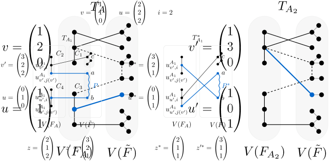
Figure 2: Example illustrating how $T_{A_{1}}^{*}$ is derived from $T_{A_{1}}$ in the proof of Lemma 3.18.

Lemma 3.18.

Let $A\in\mathcal{P}$, $i\in[k]$, $v$ and $u$ distinct vectors of $A$ such that $v_{i},u_{i}\geq 1$, and let $A_{1}=\pi_{1}(A,v,u,i)$. Then it holds that $A_{1}\preceq A$.

Proof 3.19.

Let $(v^{\prime},u^{\prime})=\pi_{1}(i,v,u)$, $\alpha\subseteq[k]^{2}$ be an edge mapping, and let $(\tilde{F},\tilde{g})$ be a fixed forest that is $\alpha$-compatible with the fixed forest of $A_{1}$, $(F_{A_{1}},f_{A_{1}})$. We need to show that $(\tilde{F},\tilde{g})$ is $\alpha$-compatible with the fixed forest of $A$, $(F_{A},f_{A})$, that is, there is an $\alpha$-spanning tree $T_{A}$ for $(\tilde{F},\tilde{g})$ and $(F_{A},f_{A})$.

By the $\alpha$-compatibility of $(\tilde{F},\tilde{g})$ and $(F_{A_{1}},f_{A_{1}})$, there is an $\alpha$-spanning tree for them. Let $P$ be a shortest path from $\{u^{A_{1}}_{v^{\prime},j}\mid j\in[k]\}$ to $\{u^{A_{1}}_{u^{\prime},j}\mid j\in[k]\}$ in $T_{A_{1}}$. Further, let $j(v^{\prime})$ be the index of the first vertex of $P$ in $\{u^{A_{1}}_{v^{\prime},j}\mid j\in[k]\}$. We let $z^{\prime}$ be a vector with $z^{\prime}_{j}=|(N_{T_{A_{1}}}(u^{A_{1}}_{v^{\prime},j})\cap V(\tilde{F}))\setminus V(P)|$ for $j\in[k]$. Observe that $z^{\prime}=v^{\prime}-\mathbf{e}_{j(v^{\prime})}$.

We distinguish two cases. First, suppose that $z\coloneqq v^{\prime}-v\leq z^{\prime}$. Then, we can apply Lemma 3.16 to $\alpha,(\tilde{F},\tilde{g}),A_{1},v^{\prime},u^{\prime},T_{A_{1}},P$, and $z$. Since, $(v,u)=(v^{\prime}-z,u^{\prime}+z)$, this yields a spanning tree satisfying the conditions of this lemma.

Otherwise, we proceed as follows. Observe that the last vertex of $P$ is $u^{A_{1}}_{u^{\prime},i}$, since $u^{\prime}=\mathbf{e}_{i}$, and observe that the edge $u^{A_{1}}_{v^{\prime},j(v^{\prime})}u^{A_{1}}_{u^{\prime},i}$ cannot be in $T_{A_{1}}$, as it is not in $\tilde{F}\oplus_{\alpha}F_{A}$. Hence $P$ counts at least three vertices; we denote the second vertex of $P$ by $a$, and the penultimate vertex of $P$ by $b$. Finally, let $c\in N_{T_{A_{1}}}(u^{A_{1}}_{v^{\prime},i})\cap V(\tilde{F})$, which exists since $v^{\prime}_{i}\geq 1$.

We obtain $P^{*}$ by replacing the first edge of $P$, $u_{v^{\prime},j(v^{\prime})}a$, with $u_{u^{\prime},j(v^{\prime})}a$, and the last edge, $bu_{u^{\prime},i}$, with $bu_{v^{\prime},i}$. Further, we obtain $T_{A_{1}}^{*}$ from $T_{A_{1}}$ by performing the same two edge substitutions, and further, we replace the edge $u^{A_{1}}_{v^{\prime},i}c$ with $u^{A_{1}}_{u^{\prime},i}c$. See Figure˜2.

We define the vectors

$$v^{\prime*} =v^{\prime}-\mathbf{e}_{j(v^{\prime})}\text{, and}$$

$$u^{\prime*} =u^{\prime}+\mathbf{e}_{j(v^{\prime})}.$$

Further, let $A_{1}^{*}=(A_{1}\setminus\langle v^{\prime},u^{\prime}\rangle)\cup\langle v^{\prime*},u^{\prime*}\rangle$. We will now argue that $T_{A_{1}}^{*}$ is an $\alpha$-spanning tree for $(\tilde{F},\tilde{g})$ and $(F_{A_{1}^{*}},f_{A_{1}^{*}})$, where we identify $u^{A_{1}}_{v^{\prime},j}=u^{A_{1}^{*}}_{v^{\prime*},j}$ and $u^{A_{1}}_{u^{\prime},j}=u^{A_{1}^{*}}_{u^{\prime*},j}$ for all $j\in[k]$, and $u^{A_{1}}_{w,j}=u^{A_{1}^{*}}_{w,j}$ for all $w\in A_{1}\setminus\langle v^{\prime},u^{\prime}\rangle$ and all $j\in[k]$. First, observe that $T_{A_{1}}-\{u^{A_{1}}_{v^{\prime},i}c,u^{A_{1}}_{v^{\prime},j(v^{\prime})}a,u^{A_{1}}_{u^{\prime},i}b\}$ consists of four connected components $C_{1},C_{2},C_{3},C_{4}$ with $c\in V(C_{1})$, $u^{A_{1}}_{v^{\prime},i},u^{A_{1}}_{v^{\prime},j(v^{\prime})}\in V(C_{2})$, $a,b\in V(C_{3})$, and $u^{A_{1}}_{u^{\prime},i}\in V(C_{4})$. Edge $u^{A_{1}}_{u^{\prime},i}c$ connects components $C_{1}$ and $C_{4}$, edge $u^{A_{1}}_{u^{\prime},j(v^{\prime})}a$ connects components $C_{4}$ and $C_{3}$, and edge $u^{A_{1}}_{v^{\prime},i}b$ connects components $C_{3}$ and $C_{2}$, yielding that $T_{A_{1}}^{*}$ is tree spanning $V(T_{A_{1}})$. Second, observe that for each edge $xy$ we replaced with $x^{\prime}y^{\prime}$, we have $\operatorname{lab}(x)=\operatorname{lab}(x^{\prime})$ and $\operatorname{lab}(y)=\operatorname{lab}(y^{\prime})$, and thus, since all replaced edges are in $E(F_{A_{1}}\oplus_{\alpha}\tilde{F})\setminus(E(F_{A_{1}})\cup E(\tilde{F}))$, so are all new edges. Third, observe that the degree of $u^{A_{1}}_{v^{\prime},j(v^{\prime})}$ in $T_{A_{1}}^{*}$ is decreased by one compared to $T_{A_{1}}$, while the degree of $u^{A_{1}}_{u^{\prime},j(v^{\prime})}$ in $T_{A_{1}}^{*}$ is increased by one compared to $T_{A_{1}}$. Thus $T_{A_{1}}^{*}$ is an $\alpha$-spanning tree for $(\tilde{F},\tilde{g})$ and $(F_{A_{1}^{*}},f_{A_{1}^{*}})$. Furthermore, observe that $P^{*}$ is a path connecting $u^{A_{1}}_{u^{\prime},j(v^{\prime})}$ and $u^{A_{1}}_{v^{\prime},i}$ in $T_{A_{1}}^{*}$. Towards applying Lemma 3.16, we define the vectors

$$(z^{\prime*})_{j} =|(N_{T^{*}_{A_{1}}}(u^{A_{1}}_{v^{\prime},j})\cap V(\tilde{F}))\setminus V(P)|\text{ for }j\in[k]\text{, and}$$

$$z^{*} =v^{\prime*}-v,$$

and observe that $z^{\prime*}=z^{\prime}-\mathbf{e}_{i}$. It remains to show that $z^{*}\leq z^{\prime*}$. By simple algebraic manipulations, the condition is equivalent to $v_{i}\geq 1$, which holds by precondition. Finally, we apply Lemma 3.16 to $\alpha,(\tilde{F},\tilde{g}),A_{1}^{*},v^{\prime*},u^{\prime*},T_{A_{1}}^{*},P^{*}$, and $z^{*}$. Since, $(v^{\prime*}-z^{*},u^{\prime*}+z^{*})=(v,u)$, we obtain a spanning tree satisfying the conditions of this lemma.

Lemma 3.20.

Let $A\in\mathcal{P}$, $i\in[k]$, $v,u$ two distinct vectors of $A$ such that $v_{i},u_{i}\geq 1$, and let $A_{2}=\pi_{2}(A,v,u,i)$. Then it holds that $A_{2}\preceq A$.

Proof 3.21.

Let $(v^{\prime},u^{\prime})=\pi_{2}(i,v,u)$, $\alpha\subseteq[k]^{2}$ be an edge mapping, and let $(\tilde{F},\tilde{g})$ be a fixed forest that is $\alpha$-compatible with the fixed forest of $A_{2}$, $(F_{A_{2}},f_{A_{2}})$. We need to show that there is an $\alpha$-spanning tree for $(\tilde{F},\tilde{g})$ and $(F_{A},f_{A})$.

By the $\alpha$-compatibility of $(\tilde{F},\tilde{g})$ and $(F_{A_{2}},f_{A_{2}})$, there is an $\alpha$-spanning tree $T_{A_{2}}$ for $(\tilde{F},\tilde{g})$ and $(F_{A_{2}},f_{A_{2}})$. Let $P$ be a shortest path from $\{u^{A_{2}}_{v^{\prime},j}\mid j\in[k]\}$ to $\{u^{A_{2}}_{u^{\prime},j}\mid j\in[k]\}$ in $T_{A_{2}}$. Further, let $j(v^{\prime})$ be the index of the first vertex of $P$ in $\{u^{A_{2}}_{v^{\prime},j}\mid j\in[k]\}$.

We aim to invoke Lemma 3.16. Let $z^{\prime}$ be a vector with $z^{\prime}_{j}=|(N_{T_{A_{2}}}(u^{A_{2}}_{v^{\prime},j})\cap V(\tilde{F}))\setminus V(P)|$ for $j\in[k]$. Further, let $z=u_{i}\cdot\mathbf{e}_{i}$. We want to show that $z\leq z^{\prime}$. Observe that this is equivalent to $z_{i}\leq z^{\prime}_{i}$. If $j(v^{\prime})\neq i$, we have $z^{\prime}_{i}=v_{i}+u_{i}$, hence $z_{i}=u_{i}\leq z^{\prime}_{i}$. If otherwise $j(v^{\prime})=i$, we have $z^{\prime}_{i}=v_{i}+u_{i}-1\geq u_{i}$ by the precondition $v_{i}\geq 1$. Hence $z_{i}=u_{i}\leq z^{\prime}_{i}$.

Finally, we apply Lemma 3.16 to $\alpha,(\tilde{F},\tilde{g}),A_{2},v^{\prime},u^{\prime},T_{A_{2}},P$, and $z$. Since, $(v^{\prime}-z,u^{\prime}+z)=(v,u)$, this yields a spanning tree satisfying the conditions of this lemma.

Lemma 3.22.

Let $A\in\mathcal{P}$, $i\in[k]$, $v,u$ two distinct vectors of $A$ such that $v_{i},u_{i}\geq 1$, $A_{1}=\pi_{1}(A,v,u,i)$, and let $A_{2}=\pi_{2}(A,v,u,i)$. Then it holds that $\{A\}\preceq\{A_{1},A_{2}\}$.

Proof 3.23.

Let $(v^{\prime}_{1},u^{\prime}_{1})=\pi_{1}(i,v,u),(v^{\prime}_{2},u^{\prime}_{2})=\pi_{2}(i,v,u)$, $\alpha\subseteq[k]^{2}$ be an edge mapping, and let $(\tilde{F},\tilde{g})$ be a fixed forest that is $\alpha$-compatible with the fixed forest of $A$, $(F_{A},f_{A})$. We need to show that there is an $\alpha$-spanning tree for $(\tilde{F},\tilde{g})$ and $(F_{A_{1}},f_{A_{1}})$, or there is an $\alpha$-spanning tree for $(\tilde{F},\tilde{g})$ and $(F_{A_{2}},f_{A_{2}})$.

By the $\alpha$-compatibility of $(\tilde{F},\tilde{g})$ and $(F_{A},f_{A})$, there is an $\alpha$-spanning tree $T_{A}$ for $(\tilde{F},\tilde{g})$ and $(F_{A},f_{A})$. Let $P$ be a shortest path from $\{u^{A}_{u,j}\mid j\in[k]\}$ to $\{u^{A}_{v,j}\mid j\in[k]\}$ in $T_{A}$. Further, let $j(u)$ be the index of the first vertex of $P$ in $\{u^{A}_{u,j}\mid j\in[k]\}$, and let $z^{\prime}$ be a vector with $z^{\prime}_{j}=|(N_{T_{A}}(u^{A}_{u,j})\cap V(\tilde{F}))\setminus V(P)|$ for $j\in[k]$.

First, suppose $j(u)=i$. Let $z=u-u_{i}\cdot\mathbf{e}_{i}$. For $j\neq i$, we have $z_{j}=z^{\prime}_{j}$, and for $j=i$, we have $z_{j}=0$. Hence $z\leq z^{\prime}$. We apply Lemma 3.16 to $\alpha,(\tilde{F},\tilde{g}),A_{1},u,v,T_{A},P$, and $z$. Since, $(u-z,v+z)=(u^{\prime}_{1},v^{\prime}_{1})$, this yields an $\alpha$-spanning tree for $(\tilde{F},\tilde{g})$ and $(F_{A_{1}},f_{A_{1}})$.

Conversely, suppose $j(u)\neq i$. Let $z=u_{i}\cdot\mathbf{e}_{i}$. For $j\neq i$, we have $z_{j}=0$, and for $j=i$, we have $z_{j}=z^{\prime}_{j}$. Hence $z\leq z^{\prime}$. We apply Lemma 3.16 to $\alpha,(\tilde{F},\tilde{g}),A_{2},u,v,T_{A},P$, and $z$. Since, $(u-z,v+z)=(u^{\prime}_{2},v^{\prime}_{2})$, this yields an $\alpha$-spanning tree for $(\tilde{F},\tilde{g})$ and $(F_{A_{2}},f_{A_{2}})$.

Combining Lemmas 3.18, 3.20 and 3.22 immediately yields the following corollary:

Corollary 3.24.

Let $A\in\mathcal{P}$, $i\in[k]$ and let $v,u$ be two distinct vectors of $A$ such that $v_{i},u_{i}\geq 1$. Then it holds that $\{A\}\simeq\{\pi_{1}(A,v,u,i),\pi_{2}(A,v,u,i)\}$.

Subroutines.

Based on the functions $\pi_{1}$ and $\pi_{2}$ defined above, we formulate the following subroutines that will be used in our algorithm.

Procedure 3.25.

We define the subroutine ReduceVector that takes as input a tuple $(A,b_{A},u)$, where $A$ is a pattern, $b_{A}$ is a big-vector mapping of $A$, and $u\in A$ is a vector of $A$, such that there exists some index $i\in[k]$ with $u\not\mathrel{\mathchoice{\ooalign{\raisebox{-1.10063pt}{$\displaystyle\widehat{}$}\cr\hbox{\set@color$\displaystyle=$}\cr}}{\ooalign{\raisebox{-1.10063pt}{$\textstyle\widehat{}$}\cr\hbox{\set@color$\textstyle=$}\cr}}{\ooalign{\raisebox{-0.77043pt}{$\scriptstyle\widehat{}$}\cr\hbox{\set@color$\scriptstyle=$}\cr}}{\ooalign{\raisebox{-0.55031pt}{$\scriptscriptstyle\widehat{}$}\cr\hbox{\set@color$\scriptscriptstyle=$}\cr}}}b_{A}(i)$ and $u_{i}\geq 1$. Let $i_{1}<\dots<i_{\ell}$ be the coordinates of $u$ such that $u\not\mathrel{\mathchoice{\ooalign{\raisebox{-1.10063pt}{$\displaystyle\widehat{}$}\cr\hbox{\set@color$\displaystyle=$}\cr}}{\ooalign{\raisebox{-1.10063pt}{$\textstyle\widehat{}$}\cr\hbox{\set@color$\textstyle=$}\cr}}{\ooalign{\raisebox{-0.77043pt}{$\scriptstyle\widehat{}$}\cr\hbox{\set@color$\scriptstyle=$}\cr}}{\ooalign{\raisebox{-0.55031pt}{$\scriptscriptstyle\widehat{}$}\cr\hbox{\set@color$\scriptscriptstyle=$}\cr}}}b_{A}(i_{j})$ and $u_{i_{j}}\geq 1$ for $j\in[\ell]$. The subroutine outputs a family $\{(A_{1},b_{A_{1}}),\dots(A_{\ell},b_{A_{\ell}})\}$, where each pair $(A_{j},b_{A_{j}})$ is defined as follows.

For $j\in[\ell]$, we obtain $A_{j}$ from the multiset $\langle\mathbf{e}_{i_{j}}\rangle$ by adding a vector $w^{v}$ for each vector $v\not\mathrel{\mathchoice{\ooalign{\raisebox{-1.10063pt}{$\displaystyle\widehat{}$}\cr\hbox{\set@color$\displaystyle=$}\cr}}{\ooalign{\raisebox{-1.10063pt}{$\textstyle\widehat{}$}\cr\hbox{\set@color$\textstyle=$}\cr}}{\ooalign{\raisebox{-0.77043pt}{$\scriptstyle\widehat{}$}\cr\hbox{\set@color$\scriptstyle=$}\cr}}{\ooalign{\raisebox{-0.55031pt}{$\scriptscriptstyle\widehat{}$}\cr\hbox{\set@color$\scriptscriptstyle=$}\cr}}}u$ in $A$, where for $t\in[k]$,

$$w^{v}_{t}=\begin{cases}v_{t}+u_{t}&\text{if $t\in\{i_{1},\dots,i_{j-1}\}$ and $v=b_{A}(t)$,}\\ v_{t}+u_{t}-1&\text{if $t=i_{j}$ and $v=b_{A}(i_{j})$,}\\ v_{t}+u_{t}&\text{if $t\in\{i_{j+1},\dots,i_{\ell}\}$ and $v=b_{A}(i_{j})$,}\\ v_{t}&\text{otherwise.}\end{cases}$$

We define $b_{A_{j}}$ as the following big-vector mapping of $A_{j}$. For $t\in[k]$, if $b_{A}(t)=u$, then $b_{A_{j}}(t)=w^{b_{A}(i_{j})}$. Otherwise, $b_{A_{j}}(t)=w^{b_{A}(t)}$.  $\blacktriangle$

Intuitively, to obtain each vector $A_{j}$, we shift the indices $i_{t}$ of $u$ for $t<j$ to the vectors $b_{A}(i_{t})$. We then shift the rest of $u$ to $b_{A}(i_{j})$, except for a single unit at the index $i_{j}$, creating a unit vector $\mathbf{e}_{i_{j}}$. We update $b_{A_{j}}$ accordingly, by pointing to the same vectors after the updates, except for indices $d$ with $b_{A}(d)=u$; these now point to $b_{A}(i_{j})$.

Equipped with the subroutine ReduceVector, we can now define the main subroutine ReduceToNice which produces an equivalent set of nice patterns for a given pattern.

Procedure 3.26.

The subroutine ReduceToNice takes a pattern $A$ that contains at most one zero vector and outputs a family $R_{A}$ of nice patterns as follows. Firstly, we fix an arbitrary big-vector mapping $b_{A}$ of $A$.

Secondly, we define $P_{0}=\{(A,b_{A})\}$. For $j\geq 1$, we define $P_{j}$ from $P_{j-1}$ as follows. We first define a set $C_{A^{\prime}}$ for every $(A^{\prime},b_{A^{\prime}})\in P_{j-1}$. If every vector $u$ in $A^{\prime}$ is a big vector, a unit vector, or a zero vector then we define $C_{A^{\prime}}=\{(A^{\prime},b_{A^{\prime}})\}$. Otherwise, let $u\in A^{\prime}$ such that $u$ is neither a big vector nor a unit vector nor a zero vector. In this case, we define $C_{A^{\prime}}=\textsc{ReduceVector}(A^{\prime},b_{A^{\prime}},u)$. Then we define $P_{j}=\bigcup_{(A^{\prime},b_{A^{\prime}})\in P_{j-1}}C_{A^{\prime}}$.

Thirdly, for the smallest value $\tilde{j}$ such that $P_{\tilde{j}}=P_{\tilde{j}-1}$, we define $P^{\prime}_{0}=P_{\tilde{j}}$. For $j^{\prime}\geq 1$, we define $P^{\prime}_{j^{\prime}}$ from $P^{\prime}_{j^{\prime}-1}$ as follows. For a pair $(A^{\prime},b_{A^{\prime}})\in P^{\prime}_{j^{\prime}}$, let $C^{\prime}_{A^{\prime}}=\{(A^{\prime},b_{A^{\prime}})\}$ if $A^{\prime}$ is a nice pattern. Otherwise, there must exist two distinct indices $i,t\in[k]$ such that $b_{A^{\prime}}(i)\not\mathrel{\mathchoice{\ooalign{\raisebox{-1.10063pt}{$\displaystyle\widehat{}$}\cr\hbox{\set@color$\displaystyle=$}\cr}}{\ooalign{\raisebox{-1.10063pt}{$\textstyle\widehat{}$}\cr\hbox{\set@color$\textstyle=$}\cr}}{\ooalign{\raisebox{-0.77043pt}{$\scriptstyle\widehat{}$}\cr\hbox{\set@color$\scriptstyle=$}\cr}}{\ooalign{\raisebox{-0.55031pt}{$\scriptscriptstyle\widehat{}$}\cr\hbox{\set@color$\scriptscriptstyle=$}\cr}}}b_{A^{\prime}}(t)$, and $(b_{A^{\prime}}(i))_{t}\geq 1$. We define $C_{A^{\prime}}=\textsc{ReduceVector}(A^{\prime},b_{A^{\prime}},b_{A^{\prime}}(i))$ and $P_{j}=\bigcup_{(A^{\prime},b_{A^{\prime}})\in P^{\prime}_{j-1}}C^{\prime}_{A^{\prime}}$. Finally, let ${\tilde{j}}^{\prime}$ be the smallest value such that $P^{\prime}_{\tilde{j}^{\prime}}=P^{\prime}_{\tilde{j}^{\prime}-1}$. Then the subroutine outputs $R_{A}=\{A^{\prime}\>:\>(A^{\prime},b_{A^{\prime}})\in P^{\prime}_{\tilde{j}^{\prime}}\}$.  $\blacktriangle$

The following two lemmas prove the correctness and bound the number of iterations of each family that the procedure ReduceToNice produces.

Lemma 3.27.

Let $A\in\mathcal{P}$ be a pattern. Then the subroutine ReduceToNice(A) produces a nice set of patterns in time $n^{\mathcal{O}(k)}$.

Proof 3.28.

Firstly, observe that ReduceVector does not increase the number of vectors in each pattern in the output compared to that in the input. Hence, throughout the subroutine, all patterns correctly have at most $n$ vectors.

Secondly, we prove that $\tilde{j}$ in ˜3.26 exists. For a pair $(A^{\prime},b_{A^{\prime}})$, let $\psi(A^{\prime},b_{A^{\prime}})$ denote the number of non-big non-unit non-zero vectors in $A^{\prime}$. Observe that if $u$ is a non-big non-unit non-zero vector of $A^{\prime}$, then for every pair $(A^{\prime\prime},b_{A^{\prime\prime}})\in\textsc{ReduceVector}(A^{\prime},b_{A^{\prime}},u)$, $\psi(A^{\prime\prime},b_{A^{\prime\prime}})<\psi(A^{\prime},b_{A^{\prime}})$, because we obtain $A^{\prime\prime}$ from $A^{\prime}$ by turning a non-big non-unit non-zero vector (i.e., $u$) into a unit vector, while keeping big vectors as big vectors and other vectors unchanged. This implies for $j\geq 1$, $\max_{(A^{\prime},b_{A^{\prime}})\in P_{j-1}}\psi(A^{\prime},b_{A^{\prime}})>\max_{(A^{\prime},b_{A^{\prime}})\in P_{j}}\psi(A^{\prime},b_{A^{\prime}})$, unless $\max_{(A^{\prime},b_{A^{\prime}})\in P_{j-1}}\psi(A^{\prime},b_{A^{\prime}})=0$. Note that when $\max_{(A^{\prime},b_{A^{\prime}})\in P_{j-1}}\psi(A^{\prime},b_{A^{\prime}})=0$, we have $P_{j-1}=P_{j}$. Hence, there must exists $\tilde{j}$ such that $P_{\tilde{j}}=P_{\tilde{j}-1}$. Further, since $A$ has at most $n$ vectors, the smallest such $\tilde{j}$ satisfies $\tilde{j}\leq n$.

Thirdly, we prove that $\tilde{j}^{\prime}$ in ˜3.26 exists. For a pair $(A^{\prime},b_{A^{\prime}})$, we call a big vector $u$ of $A^{\prime}$ bad if there exists $i\in[k]$ such that $u_{i}\geq 1$ and $u\not\mathrel{\mathchoice{\ooalign{\raisebox{-1.10063pt}{$\displaystyle\widehat{}$}\cr\hbox{\set@color$\displaystyle=$}\cr}}{\ooalign{\raisebox{-1.10063pt}{$\textstyle\widehat{}$}\cr\hbox{\set@color$\textstyle=$}\cr}}{\ooalign{\raisebox{-0.77043pt}{$\scriptstyle\widehat{}$}\cr\hbox{\set@color$\scriptstyle=$}\cr}}{\ooalign{\raisebox{-0.55031pt}{$\scriptscriptstyle\widehat{}$}\cr\hbox{\set@color$\scriptscriptstyle=$}\cr}}}b_{A^{\prime}}(i)$. Let $\beta(A^{\prime},b_{A^{\prime}})$ denote the number of big vectors in $A^{\prime}$. Now suppose that $A^{\prime}$ contains only big vectors, unit vectors, and at most one zero vector. If $A^{\prime}$ is not nice, there must exist two distinct indices $i,t\in[k]$ such that $b_{A^{\prime}}(i)\not\mathrel{\mathchoice{\ooalign{\raisebox{-1.10063pt}{$\displaystyle\widehat{}$}\cr\hbox{\set@color$\displaystyle=$}\cr}}{\ooalign{\raisebox{-1.10063pt}{$\textstyle\widehat{}$}\cr\hbox{\set@color$\textstyle=$}\cr}}{\ooalign{\raisebox{-0.77043pt}{$\scriptstyle\widehat{}$}\cr\hbox{\set@color$\scriptstyle=$}\cr}}{\ooalign{\raisebox{-0.55031pt}{$\scriptscriptstyle\widehat{}$}\cr\hbox{\set@color$\scriptscriptstyle=$}\cr}}}b_{A^{\prime}}(t)$, and $(b_{A^{\prime}}(i))_{t}\geq 1$. Further, for any pair $(A^{\prime\prime},b_{A^{\prime\prime}})\in\textsc{ReduceVector}(A^{\prime},b_{A^{\prime}},b_{A^{\prime}}(i))$, $A^{\prime\prime}$ has only big vectors, unit vectors, and at most one zero vector, and $\beta(A^{\prime\prime},b_{A^{\prime\prime}})<\beta(A^{\prime},b_{A^{\prime}})$, because we obtain $A^{\prime\prime}$ from $A^{\prime}$ by turning a (bad) big vector into a non-big unit vector.

Now, this implies that for $j^{\prime}\geq 1$, any pair $(A^{\prime},b_{A^{\prime}})\in P^{\prime}_{j^{\prime}}$ satisfies $A^{\prime}$ contains only big vectors, unit vectors, and at most one zero vector. Further, for $j^{\prime}\geq 0$, let $\gamma(j^{\prime})$ be the largest value $\beta(A^{\prime},b_{A^{\prime}})$ among all $(A^{\prime},b_{A^{\prime}})\in P^{\prime}_{j^{\prime}}$ such that $A^{\prime}$ has a bad vector; if there is no such $(A^{\prime},b_{A^{\prime}})$, we define $\gamma(j^{\prime})=0$. Then the preceding paragraph implies that $\gamma(j^{\prime})>\gamma(j^{\prime}+1)$, unless $\gamma(j^{\prime})=0$. Hence, there must exists $\tilde{j}^{\prime}$ such that $P^{\prime}_{\tilde{j}^{\prime}}=P^{\prime}_{\tilde{j}^{\prime}-1}$. Further, since $\gamma(0)\leq k$, the smallest such $\tilde{j}^{\prime}$ satisfies $\tilde{j}^{\prime}\leq k$.

Then the correctness of the subroutine follows, since by definition, all $(A^{\prime},b_{A^{\prime}})\in P^{\prime}_{\tilde{j}^{\prime}}$ satisfy that $A^{\prime}$ is a nice pattern.

Finally, we prove the runtime. Each call of ReduceVector creates a family of at most $k$ objects and runs in time $\poly(n,k)$. Since there are at most $n$ iterations in the second step and at most $k$ iterations in the third step of ˜3.26, it follows that the whole subroutine runs in time $\poly(n,k)(n+k)^{k}=n^{\mathcal{O}(k)}$.

Lemma 3.29.

For any pattern $A\in\mathcal{P}$, we have $\{A\}\simeq\textsc{{ReduceToNice}}(A)$.

Proof 3.30.

We show that for any $(A,b_{A})$ and $u\in A$ where $A$ is a pattern and $b_{A}$ is a big-vector mapping of $A$, it holds that $\{A\}\simeq\{A^{\prime}\>:\>(A^{\prime},b_{A^{\prime}})\in\textsc{ReduceVector}(A,b_{A},u)\}$. The lemma will then follow.

We use the same notation as in ˜3.26. For $j\in[\ell]$, let $u^{j}=u-\sum_{t<i_{j}}u_{i}\cdot\mathbf{e}_{i}$ (i.e., $u^{j}$ is the vector obtained from $u$ be replacing all entries up to (but not including) the $i_{j}$ entry with zero). For $j\in[\ell]$, let $D_{j}$ be the pattern $A_{j}\setminus\langle\mathbf{e}_{i_{j}},w^{b_{A}(i_{j})}\rangle\cup\langle u^{j},w^{b_{A}(i_{j})}-u^{j}+\mathbf{e}_{i_{j}}\rangle$. Note that $u^{1}=u$ and $D_{1}=A$.

It holds for $j\in[\ell-1]$ that $A_{j}=\pi_{1}(D_{j},b_{D_{j}}(i_{j}),u^{j},i_{j})$, and $D_{j+1}=\pi_{2}(D_{j},b_{D_{j}}(i_{j}),u^{j},i_{j})$. Then by Corollary˜3.24, $\{D_{j}\}\simeq\{A_{j},D_{j+1}\}$. Observe that $A_{\ell}=\pi_{1}(D_{\ell},b_{D_{\ell}}(i_{\ell}),u^{\ell},i_{\ell})=\pi_{2}(D_{\ell},b_{D_{\ell}}(i_{\ell}),u^{\ell},i_{\ell})$. Hence, by Corollary˜3.24, $\{D_{\ell}\}\simeq\{A_{\ell}\}$. It follows that $\{A\}=\{D_{1}\}\simeq\{A_{1},D_{2}\}\simeq\dots\simeq\{A_{1},\dots,A_{\ell}\}$. The lemma then follows.

Algorithm.

Before defining the algorithm, we describe an auxiliary operator that corresponds to relabeling vertices in the NLC-expression, i.e., it describes how the pattern changes after relabeling.

Definition 3.31.

For a relabeling function $\beta:[k]\to[k]$ and for $v\in\mathbb{N}^{k}$, we define $\rho_{\beta}(v)=v^{\prime}$, where $v^{\prime}_{i}=\sum\limits_{j\in\beta^{-1}(i)}v_{j}$. Given a pattern $A$, we define $\rho_{\beta}(A)=\langle\rho_{\beta}(v)\colon v\in A\rangle$.

Now, we describe our algorithm. Intuitively, at each join node of the NLC-decomposition, we guess the partial solutions in its children, as well as which of the newly added edges we will use. Next, we execute the relabeling procedure. Finally, we make our record nice.

Algorithm 3.32.

For each $x\in\mathcal{V}$, we define the families $T_{x}\subseteq\mathcal{P}^{*}$ recursively over $\mathcal{T}$ as follows. For an initial node $\bullet_{i}$, let $v$ be the only vertex of $\bullet_{i}$; we define $T_{x}=\{\langle t\cdot\mathbf{e}_{i}\rangle:\>t\in D(v)\}$. Let $G_{x}=G_{x_{1}}\oplus_{\alpha}^{\beta}G_{x_{2}}$. We define $P_{x}=\{(A_{1},A_{2})\colon A_{1}\in T_{x_{1}},A_{2}\in T_{x_{2}}\}$, and derive $T^{(1)}_{x}$ from $P_{x}$ as follows. For each pair $(A_{1},A_{2})\in P_{x}$, let $\hat{G}=F_{A_{1}}\oplus_{\alpha}F_{A_{2}}$, and let $\hat{E}=E(\hat{G})\setminus\big{(}E(F_{A_{1}})\cup E(F_{A_{2}})\big{)}$. For each $E^{\prime}\subseteq\hat{E}$, let $G^{\prime}$ be the graph resulting from the disjoint union of $F_{A_{1}}$ and $F_{A_{2}}$ by adding $E^{\prime}$. If it holds that $G^{\prime}$ is acyclic and $\operatorname{patt}(G^{\prime},(f_{A_{1}}\cup f_{A_{2}})-\mathrm{deg}_{E^{\prime}})$ is a pattern with at most one zero vector, then we add this pattern to $T^{(1)}_{x}$. Next, we define $T^{(2)}_{x}=\{\rho_{\beta}(A)\colon A\in T^{(1)}_{x}\}$. Finally, we set $T_{x}=\bigcup_{A\in T^{(2)}_{x}}\textsc{ReduceToNice}(A)$.  $\blacktriangle$

Lemma 3.33 shows that the computed table entries are equivalent to records at each node:

Lemma 3.33.

It holds for each $x\in\mathcal{V}$ that $T_{x}$ is equivalent to the record $\mathcal{R}_{x}$, i.e., $T_{x}\simeq\mathcal{R}_{x}$.

Proof 3.34.

We prove this lemma by induction over $\mathcal{T}$. Let $x$ be a $\bullet_{i}$ node and let $v$ be the only vertex of $G_{x}$. It is easy to see that the set of partial solutions is $\{(G_{x},t):\>t\in D(v)\}$ (where, by slight abuse of notation, each integer $t\in D(v)$ denotes the constant function $\{v\}\to\mathbb{N}$ defined by $t(v)=t$), and that $\mathcal{R}_{x}=\{\langle t\cdot\mathbf{e}_{i}\rangle:\>t\in D(v)\}=T_{x}$.

Now suppose that $x\in\mathcal{V}$ has children $x_{1}$ and $x_{2}$. By the induction hypothesis, $T_{x_{1}}\simeq\mathcal{R}_{x_{1}}$ and $T_{x_{2}}\simeq\mathcal{R}_{x_{2}}$. Note that by Lemma 3.29, it suffices to show that $T_{x}^{(2)}\simeq\mathcal{R}_{x}$. Let $G_{x}^{\prime}=G_{x_{1}}\oplus_{\alpha}G_{x_{2}}$ and let $\mathcal{R}_{x}^{\prime}$ be the record of $(G_{x}^{\prime},D_{x})$. Let $\alpha_{R}=\{(i,j)\in[k]^{2}:\>(j,i)\in\alpha\}$.

Claim 3.35.

We have $\mathcal{R}_{x}^{\prime}\simeq T_{x}^{(1)}$.

Let $R\in\mathcal{R}^{\prime}_{x}$ and let $(F,g)$ be a partial solution of $(G_{x}^{\prime},D_{x})$ such that $R=\operatorname{patt}(F,g)$. Let $\alpha^{\prime}\in[k]^{2}$ and let $(F^{\prime},g^{\prime})$ be a fixed forest that is $\alpha^{\prime}$-compatible with the canonical fixed forest of $R$. By ˜3.9, $(F^{\prime},g^{\prime})$ is $\alpha^{\prime}$-compatible with $(F,g)$. Let $T$ be the $\alpha^{\prime}$-spanning forest for $(F^{\prime},g^{\prime})$ and $(F,g)$.

We aim to construct an entry in $T_{x}^{(1)}$ that $(F^{\prime},g^{\prime})$ is $\alpha^{\prime}$-compatible with. To facilitate this construction, we will (temporarily) introduce $k$ new labels and we will work with $2k$-graphs instead of $k$-graphs.

Let $F^{\prime}_{\text{rel}}$ be the labeled graph obtained by relabeling the vertices of $F^{\prime}$ (and keeping the edge set the same) with $\text{rel}:i\mapsto i+k$. We define $\alpha^{\prime}_{\text{rel}}=\{(i+k,j):\>(i,j)\in\alpha^{\prime}\}$. Note that $(F^{\prime}_{\text{rel}},g^{\prime})$ is $\alpha^{\prime}_{\text{rel}}$-compatible with $(F,g)$, with $\alpha^{\prime}_{\text{rel}}$-spanning tree $T$.

Let $F_{1}=F\cap G_{x_{1}}$, $F_{2}=F\cap G_{x_{2}}$. Let $g_{1}:V_{x_{1}}\rightarrow\mathbb{N}$, $g_{2}:V_{x_{2}}\rightarrow\mathbb{N}$ be defined as $g_{1}=g+\mathrm{deg}_{F}-\mathrm{deg}_{F_{1}}$, $g_{2}=g+\mathrm{deg}_{F}-\mathrm{deg}_{F_{2}}$. Note that $(F_{1},g_{1})$ is a partial solution of $(G_{x_{1}},D_{x_{1}})$ and $(F_{2},g_{2})$ is a partial solution of $(G_{x_{2}},D_{x_{2}})$, so $\operatorname{patt}(F_{1},g_{1})\in\mathcal{R}_{x_{1}}$ and $\operatorname{patt}(F_{2},g_{2})\in\mathcal{R}_{x_{2}}$. Intuitively, our goal is to find the entry in $P_{x}$ that corresponds to $(F_{1},g_{1})$ and $(F_{2},g_{2})$ and to find the edge set that needs to be added between this pair.

Let $H_{1}$ be the labeled forest containing vertices $V(F_{2})\cup V(F^{\prime}_{\text{rel}})$, and edges $\{uv\in E(T):\>u\not\in V(F_{1}),\>v\not\in V(F_{1})\}$ (i.e., the forest obtained by deleting the edges of $F_{1}$ from $T$). The graph $H_{1}\oplus_{\alpha_{R}\cup\alpha^{\prime}_{\text{rel}}}F_{1}$ has vertices $V(F_{2})\cup V(F^{\prime}_{\text{rel}})\cup V(F_{1})$. Since $\alpha_{R}$ and $\alpha^{\prime}_{\text{rel}}$ are disjoint, its edge set is obtained by taking edges between $F_{2}$ and $F_{1}$ corresponding to $\alpha_{R}$ and edges between $F^{\prime}_{\text{rel}}$ and $F_{1}$ corresponding to $\alpha_{\text{rel}}^{\prime}$. Thus $T$ is a spanning tree in $H_{1}\oplus_{\alpha_{R}\cup\alpha_{\text{rel}}^{\prime}}F_{1}$.

Therefore, $(H_{1},(\mathrm{deg}_{T}-\mathrm{deg}_{F_{1}})\cup(\mathrm{deg}_{T}-\mathrm{deg}_{H_{1}}))$ is $(\alpha_{R}\cup\alpha^{\prime}_{\text{rel}})$-compatible with $(F_{1},g_{1})$. Since $\operatorname{patt}(F_{1},g_{1})\in\mathcal{R}_{x_{1}}$ and $\mathcal{R}_{x_{1}}\simeq T_{x_{1}}$ (by induction hypothesis), there is an element $A_{1}\in T_{x_{1}}$ such that $(H_{1},(\mathrm{deg}_{T}-\mathrm{deg}_{F_{1}})\cup(\mathrm{deg}_{T}-\mathrm{deg}_{H_{1}}))$ is $(\alpha_{R}\cup\alpha^{\prime}_{\text{rel}})$-compatible with $(F_{A_{1}},f_{A_{1}})$. Let $T_{1}$ be the corresponding $(\alpha_{R}\cup\alpha^{\prime}_{\text{rel}})$-spanning tree.

Let $H_{2}$ be the labeled forest with vertex set $V(F_{A_{1}})\cup V(F^{\prime}_{\text{rel}})$ and edges $\{uv\in E(T_{1}):\>u\not\in V(F_{2}),v\not\in V(F_{2})\}$ (i.e., the forest obtained by deleting the edges of $F_{2}$ from $T_{1}$). Analogously, $(H_{2},(\mathrm{deg}_{T_{1}}-\mathrm{deg}_{F_{2}})\cup(\mathrm{deg}_{T_{1}}-\mathrm{deg}_{H_{2}}))$ is $\alpha\cup\alpha_{\text{rel}}^{\prime}$-compatible with $(F_{2},g_{2})$, and there is an element $A_{2}\in T_{x_{2}}$ such that $(H_{2},(\mathrm{deg}_{T_{1}}-\mathrm{deg}_{F_{2}})\cup(\mathrm{deg}_{T_{1}}-\mathrm{deg}_{H_{2}}))$ is $\alpha\cup\alpha^{\prime}_{\text{rel}}$-compatible with $(F_{A_{2}},f_{A_{2}})$. Let $T_{2}$ be the corresponding $(\alpha\cup\alpha^{\prime}_{\text{rel}})$-spanning tree.

Now we obtained a pair $(A_{1},A_{2})\in P_{x}$, and it remains to describe the set of edges that need to be added. Let $E^{\prime}=\{uv\in E(T_{2}):\>u\in V(F_{A_{1}}),v\in V(F_{A_{2}})\}$. By construction, the labels of endpoints of edges in $E^{\prime}$ belong to $\alpha\cup\alpha^{\prime}_{\text{rel}}$. However, the vertices of $F_{A_{1}}$ and $F_{A_{2}}$ do not have labels in $\{k+1,\dots,2k\}$, so the endpoints of all edges in $E^{\prime}$ have labels in $\alpha$, i.e., $E^{\prime}\subseteq E(F_{A_{1}}\oplus_{\alpha}F_{A_{2}})\setminus(E(F_{A_{1}})\cup E(F_{A_{2}}))$.

Let $G^{\prime}$ be the graph obtained by adding edges $E^{\prime}$ to the disjoint union of $F_{A_{1}}$ and $F_{A_{2}}$. Since $G^{\prime}$ is a subgraph of $T_{2}$, it is acyclic. Let $p=(G^{\prime},(f_{A_{1}}\cup f_{A_{2}})-\mathrm{deg}_{E^{\prime}})$. It is easy to see that $\operatorname{patt}(p)$ is a pattern with at most one zero vector, so $\operatorname{patt}(p)\in T_{x}^{(1)}$. Note that $(F^{\prime}_{\text{rel}},g^{\prime})$ is $\alpha^{\prime}_{\text{rel}}$-compatible with $p$, so $(F^{\prime},g^{\prime})$ is $\alpha^{\prime}$-compatible with $p$. By construction, the labels $k+1,\dots,2k$ do not appear in $G^{\prime}$, i.e., we can safely delete them and consider $G^{\prime}$ a $k$-labeled graph.

The proof in the other direction can be obtained by reversing the direction of implications.

Claim 3.36.

We have $\mathcal{R}_{x}\simeq T_{x}^{(2)}$.

Let $R\in\mathcal{R}_{x}$ be a pattern and let $(H,h)$ be a partial solution with $\operatorname{patt}(H,h)=R$. Let $\alpha\in[k]^{2}$ and let $(F,g)$ be a fixed forest that is $\alpha$-compatible with $(H,h)$ and let $T$ be the corresponding $\alpha$-spanning tree. We aim to construct an element of $T_{x}^{(2)}$ such that $(F,g)$ is $\alpha$-compatible with its canonical fixed forest.

Let $(H_{\varphi},h)$ be the partial solution with pattern in $\mathcal{R}_{x}^{\prime}$ such that $H$ is obtained by applying relabeling $\beta$ to $H_{\varphi}$. Let $\alpha^{\prime}=\{(i,j):\>(i,\beta(j))\in\alpha\}$. Note that $F\oplus_{\alpha^{\prime}}H_{\varphi}$ has the same edge set as $F\oplus_{\alpha}H$, so $(F,g)$ is $\alpha^{\prime}$-compatible with $(H_{\varphi},h)$ (with $\alpha^{\prime}$-spanning tree $T$). Since $\operatorname{patt}(H_{\varphi},h)\in\mathcal{R}_{x}^{\prime}$ and $\mathcal{R}_{x}^{\prime}\simeq T_{x}^{(1)}$, there is a pattern $A\in T_{x}^{(1)}$ such that $(F,g)$ is $\alpha^{\prime}$-compatible with $(F_{A},f_{A})$. Let $T_{1}$ be the corresponding $\alpha^{\prime}$-spanning tree. Let $B=\rho_{\beta}(A)$. Note that $B\in T_{x}^{(2)}$. It remains to prove that $(F,g)$ is $\alpha$-compatible with $B$. Note that $F_{B}$ is the same labeled forest as $F_{A}$, since $\rho_{\beta}$ only affects the requirement function. Let us construct an $\alpha$-spanning $T_{2}$ in $F\oplus_{\alpha}F_{A}$ as follows. For each edge $uv\in T_{1}$, where $u\in V(F)$ and $v\in V(F_{A})$, we do the following. Let $\operatorname{lab}_{F_{A}}(v)=i$ and let $C$ be the connected component of $v$ in $F_{A}$. We add to $T_{2}$ the edge between $u$ and the unique vertex in $C$ with label $\beta(i)$. Note that, since the edge $uv$ had labels $(\operatorname{lab}_{F}(u),i)\in\alpha^{\prime}$, the newly constructed edge of $T_{2}$ has labels $(\operatorname{lab}_{F}(u),\beta(i))\in\alpha$. Finally, we add to $T_{2}$ all edges inside $F$ and $F_{A}$. It is easy to see that $T_{2}$ is a spanning tree in $F\oplus_{\alpha}F_{A}$. For each vertex $u\in V(F)$, $\mathrm{deg}_{T_{2}}(u)=\mathrm{deg}_{T_{1}}(u)$, and for each vertex $v\in V(F_{A})$, $\mathrm{deg}_{T_{2}}(v)$ is equal to the sum of $\mathrm{deg}_{T_{1}}(v^{\prime})$, where $v^{\prime}$ is a vertex in the same connected component as $v$ and $\operatorname{lab}_{F_{A}}(v^{\prime})\in\beta^{-1}(\operatorname{lab}_{F_{A}}(v))$. Thus $(F,g)$ is $\alpha$-compatible with $B$.

The other direction can be obtained by reversing the direction of implications.

Corollary 3.37 tells us that the input is a YES-instance if and only if the table entry at the root contains the pattern $\langle\mathbf{0}\rangle$. Informally, the pattern $\langle\mathbf{0}\rangle$ corresponds to a partial solution with one connected component, where all degree constraints are satisfied, i.e., a solution.

Corollary 3.37.

The instance $(G,D)$ is a YES-instance if and only if $T_{r}$ contains a $\langle\mathbf{0}\rangle$.

Proof 3.38.

It is easy to see that $\langle\mathbf{0}\rangle$ is the only pattern that is $\emptyset$-compatible with the empty graph.

Suppose $\langle\mathbf{0}\rangle\in T_{r}$. Since $T_{r}\simeq R_{r}$ and $\mathbf{0}$ is $\emptyset$-compatible with the empty graph, there is an element in $\mathcal{R}_{r}$ that is $\emptyset$-compatible with the empty graph, i.e., $\langle\mathbf{0}\rangle\in\mathcal{R}_{r}$. The partial solution that corresponds to $\langle\mathbf{0}\rangle$ is a forest in $G$ with one connected component that satisfies all degree requirements, i.e., it is a solution to our input instance.

For the other direction, let $T$ be a spanning tree in $G$ that satisfies all degree requirements. Then $\operatorname{patt}(T,\mathbf{0})=\langle\mathbf{0}\rangle\in\mathcal{R}_{r}$. By the same argument as above, $\langle\mathbf{0}\rangle\in T_{r}$.

Finally, we bound the running time of our algorithm:

Lemma 3.39.

Algorithm 3.32 runs in time $n^{\mathcal{O}(k)}$.

Proof 3.40.

For a join node $x\in\mathcal{V}$, let $x_{1},x_{2}\in\mathcal{V}$ be its children. We claim that we can compute $T_{x}$ in time $n^{\mathcal{O}(k)}$ given $T_{x_{1}}$ and $T_{x_{2}}$.

Firstly, by construction and Lemma˜3.27, $T_{x_{1}}$ and $T_{x_{2}}$ are sets of nice patterns. By Observation 3.14, this implies that $|T_{x_{1}}|,|T_{x_{2}}|\leq n^{\mathcal{O}(k)}$. Therefore, $|P_{x}|\leq n^{\mathcal{O}(k)}$.

Secondly, we bound the size of $T^{(1)}_{x}$. A component of $F_{A_{1}}$ or $F_{A_{2}}$ is a unit component, if it corresponds to a unit vector in $A_{1}$ or $A_{2}$. Similarly, a component is a big component and zero component, if it corresponds to a big vector and zero vector, respectively. By the definition of a nice pattern, there are $\mathcal{O}(k)$ big components, $\mathcal{O}(n)$ unit components, and at most one zero component. For a subset $E^{\prime}\subset\hat{E}$, if it contains an edge between two unit components, then the resulting graph $G^{\prime}$ contains a zero component. Hence, in order for $G^{\prime}$ to be added to $T^{(1)}_{x}$, except for at most one edge $e$ connecting two unit components, all other edges in $E^{\prime}$ have to be adjacent to a big component. There are $\mathcal{O}(n^{2})$ choices of the edge $e$ between two unit components. For each of the other $\mathcal{O}(n)$ unit components, note that it can only be connected with at most one other component, which has to be a big component. Therefore, there are $\mathcal{O}(k)$ choices of the big component that it can connect to. Additionally, since $G^{\prime}$ has to be acyclic in order to be added to $T^{(1)}_{x}$, among $\mathcal{O}(k)$ big components, $E$ can contain only $\mathcal{O}(k)$ edges connecting them, among $\mathcal{O}(k^{2})$ possible edges. Hence, the total number of graphs that can be added to $T^{(1)}_{x}$ is $n^{\mathcal{O}(k)}k^{\mathcal{O}(k)}=n^{\mathcal{O}(k)}$.

Thirdly, since the relabeling operation does not increase the number of vectors, we have $|T^{(2)}_{x}|\leq|T^{(1)}_{x}|$.

Finally, to obtain $T_{x}$, we perform $|T^{(2)}_{x}|$ calls of ReduceToNice, each of which takes time $n^{\mathcal{O}(k)}$, by Lemma˜3.27. Hence, in total, this step takes time $n^{\mathcal{O}(k)}$.

The lemma then follows.

4 Upper Bound Techniques

Except for our clique-width algorithm, all our upper bounds rely on the Cut&Count technique that counts the number of weighted solutions (modulo two) in the given running time. We make use of the isolation lemma to reduce the decision version of this problem to the counting (modulo two) version with high probability.

Cut and Count.

Let $(G=(V,E),w,D,B)$ be a weighted Set of Degrees MST instance, with $n=|V|$ and $m=|E|$. Further, let $d(v)=\max D(v)$ for each vertex $v\in V$, and let $r=\max_{v\in V}d(v)$ be the maximum requirement over all vertices. Next, let $W=\max_{e\in E}w(e)$, $\overline{W}=[(n-1)\cdot W]_{0}$, and $\overline{M}=[m]_{0}$. We will later fix a value $Z\in\mathbb{N}$ that is bounded polynomially in $m$, and a second weight function $w^{\prime}:E\rightarrow[Z]_{0}$. We set $\overline{Z}=[(n-1)\cdot Z]_{0}$. Similar to [9], we define the family of all solutions, relaxed solutions, and consistent cuts.

A solution is a set of edges $F\subseteq E$, such that $G[F]$ is a tree, and $\mathrm{deg}_{F}(v)\in D(v)$ for each $v\in V$. Let $\mathcal{S}$ be the family of all solutions. We define families of weighted solutions, where for $\omega_{1}\in\overline{W}$ and $\omega_{2}\in\overline{Z}$ we define: $\mathcal{S}[\omega_{1},\omega_{2}]=\big{\{}F\in\mathcal{S}\colon w(F)=\omega_{1},w^{\prime}(F)=\omega_{2}\}$. Our goal is to compute the parity of $\mathcal{S}[\omega_{1},\omega_{2}]$ for all values $\omega_{1},\omega_{2}$. We achieve this by counting consistent cuts (defined below) using the Cut&Count technique.

We define a relaxed solution as a set of edges $F\subseteq E$, where $|F|=n-1$, and for each vertex $v$ it holds that $\mathrm{deg}_{F}(v)\in D(v)$. Let $\mathcal{R}$ be the family of all relaxed solutions. Similarly, we define families of weighted relaxed solutions: $\mathcal{R}[\omega_{1},\omega_{2}]=\big{\{}F\in\mathcal{R}\colon w(F)=\omega_{1},w^{\prime}(F)=\omega_{2}\}$.

Definition 4.1.

Given a set of edges $F\in\mathcal{R}$, a consistent cut of $G[F]$ is a pair $(F,c)$, where $c:V\rightarrow\{\boldsymbol{L},\boldsymbol{R}\}$ is a mapping, such that for each connected component $C\in\cc(G[F])$ it holds that $|c(C)|=1$. For a relaxed solution $F\in\mathcal{R}$, let $\mathcal{C}(F)$ be the family of all consistent cuts of $F$. Let $\mathcal{C}$ be the family of all consistent cuts of all relaxed solutions. We define families of consistent cuts of weighted relaxed solutions $\mathcal{C}[\omega_{1},\omega_{2}]$ as follows:

$$\mathcal{C}[\omega_{1},\omega_{2}]=\big{\{}(F,c)\in\mathcal{R}[\omega_{1},\omega_{2}]\times\{\boldsymbol{L},\boldsymbol{R}\}^{V}\colon(F,c)\text{ is a consistent cut of }G[F]\big{\}}.$$

Furthermore, let $C[\omega_{1},\omega_{2}]=\big{|}\mathcal{C}[\omega_{1},\omega_{2}]\big{|}$.

We use a slightly modified version of the Cut&Count technique that was first used by Hegerfeld and Kratsch [22]. They prove the following result:

Lemma 4.2 ([22]).

It holds that $C[\omega_{1},\omega_{2}]\equiv_{4}2\cdot\big{|}\mathcal{S}[\omega_{1},\omega_{2}]\big{|}$.

Proof 4.3.

It holds for each $F\in\mathcal{R}$ that if $G[F]$ is connected, then $G[F]$ is acyclic as well, since $|F|=n-1$. Hence, it holds that $F\in\mathcal{S}$ if and only if $F\in\mathcal{R}$ and $G[F]$ is connected.

Let $F\in\mathcal{R}$. Since all vertices of each connected component must be assigned one of the two values $\boldsymbol{L}$ and $\boldsymbol{R}$, and since we can choose this value independently for each connected component, it holds that $|\mathcal{C}(F)|=2^{|\cc(G[F])|}$. Therefore, it follows that

$$C[\omega_{1},\omega_{2}]={\sum\limits_{\begin{subarray}{c}F\in\mathcal{R}[a,\omega_{1},\omega_{2}]\\ G[F]\text{ is connected}\end{subarray}}}2+{\sum\limits_{\begin{subarray}{c}F\in\mathcal{R}[\omega_{1},\omega_{2}]\\ G[F]\text{ is disconnected}\end{subarray}}}2^{|\cc(G[F])|}\equiv_{4}2\cdot\big{|}\mathcal{S}[\omega_{1},\omega_{2}]\big{|},$$

where the congruence holds, since the second summand is always congruent to zero modulo four, as $G[F]$ contains at least two connected components whenever $G[F]$ is disconnected.

In other words, it holds that $C[\omega_{1},\omega_{2}]$ is always even, and that $\big{|}\mathcal{S}[\omega_{1},\omega_{2}]\big{|}$ is odd, if and only if $C[\omega_{1},\omega_{2}]\equiv_{4}2$ (i.e., if $C[\omega_{1},\omega_{2}]/2$ is odd). Hence, one can decide the parity of $|\mathcal{S}[\omega_{1},\omega_{2}]|$ by computing $C[\omega_{1},\omega_{2}]$ modulo 4. We use the isolation lemma to show that this suffices to solve the decision version with high probability.

Isolation Lemma.

We say that a function $\omega:U\rightarrow\mathbb{Z}$ isolates a set family $\mathcal{F}\subseteq 2^{U}$ if there exists a unique $S^{\prime}\in\mathcal{F}$ with $\omega(S^{\prime})=\min_{S\in\mathcal{F}}\omega(S)$. Mulmuley et al. [32] showed that one can isolate any set family with high probability, by choosing the weight function uniformly at random in a large enough space.

Lemma 4.4 ([32]).

Let $\mathcal{F}\subseteq 2^{U}$ be a set family over a universe $U$ with $|\mathcal{F}|>0$, and let $N>|U|$ be an integer. For each $u\in U$, choose a weight $\omega(u)\in\{1,2,\dots N\}$ uniformly and independently at random. Then it holds that $P[\omega\text{ isolates }\mathcal{F}]\geq 1-|U|/N$.

Based on their result, we prove the following lemma:

Lemma 4.5.

Let $Z=2\cdot m$. We choose $w^{\prime}:E\rightarrow[Z]_{0}$, where we choose $w^{\prime}(e)$ independently and uniformly at random for each edge $e\in E$. Let $\omega_{1}\in\overline{W}$ be the smallest weight of a solution $F\in\mathcal{S}$. Then with probability at least $1/2$, there exists a value $\omega_{2}\in\overline{Z}$ such that $\mathcal{S}[\omega_{1},\omega_{2}]$ contains a single solution only.

Proof 4.6.

Let $U=E$, and $\mathcal{F}=\{F\in\mathcal{S}\colon w(F)=\omega_{1}\}$. By ˜4.4, it holds that $P[\omega\text{ isolates }\mathcal{F}]\geq 1-|E|/Z=1/2$.

In our remaining algorithmic results, we show how to compute the values $C[\omega_{1},\omega_{2}]$ (modulo $4$) in the given running time.

5 Treewidth

Since our lower bound for treewidth follows directly from the one for pathwidth, our aim in this section is to obtain the following algorithmic upper bound for Set of Degrees MST:

Theorem 5.1.

There exists a Monte-Carlo algorithm that, given an instance $(G,w,D,B)$ of the weighted Set of Degrees MST problem together with a nice tree decomposition of $G$ of width $\operatorname{tw}$, solves the problem in time $\mathcal{O}^{*}\big{(}(2r+2)^{\operatorname{tw}}\big{)}$. The algorithm produces false negatives only and outputs the right answer with probability at least one half.

Towards establishing Theorem 5.1, let $(\mathcal{T},\mathcal{B})$ be a nice tree decomposition of $G$ of width $\operatorname{tw}$ rooted at $r$. Intuitively, our algorithm uses records to store the following information about each vertex $v$ in the bag: on which side of the consistent cut it lies (L or R; see Definition 4.1), and the degree of $v$ that has been used up so far. Our aim is to compute the size of the set $\mathcal{C}[\circ,\circ]$ modulo $4$ in order to apply Lemma 4.2. At its core, we can formalize it as follows:

Algorithm 5.2.

For a vertex set $S$, we call a mapping $c:S\rightarrow\{\boldsymbol{L},\boldsymbol{R}\}$ a coloring. For $x\in\mathcal{V}$, we define the family of indices at $x$ as $\mathcal{I}_{x}=([r]_{0})^{B_{x}}\times\{\boldsymbol{L},\boldsymbol{R}\}^{B_{x}}$.

Let $x\in\mathcal{V}$, and let $x^{\prime}$ be the child of $x$ if $x$ has a single child, or $x_{1}$ and $x_{2}$ be the children of $x$ if it has two. For $(a,\omega_{1},\omega_{2})\in\overline{M}\times\overline{W}\times\overline{Z}$, we define the tables $T_{x}[a,\omega_{1},\omega_{2}]\in(\mathbb{Z}_{4})^{\mathcal{I}_{x}}$, where for $(f,c)\in\mathcal{I}_{x}$ we define the value of $T_{x}[a,\omega_{1},\omega_{2}][f,c]$ as follows:

• Leaf node introducing vertex $v$: Let $\phi$ be the pair $(\emptyset_{v},\emptyset_{c})$, where $\emptyset_{v}$ is a vector over an empty set, and $\emptyset_{c}$ is the empty coloring. We define $T_{x}[0,0,0][\phi]=1$, and $T_{x}[a,\omega_{1},\omega_{2}][f,c]=0$ for all other values $a,\omega_{1},\omega_{2},f,c$.

• Introduce vertex $v$: Let $f^{\prime}$ and $c^{\prime}$ be the restrictions of $f$ and $c$ to $B_{x^{\prime}}$. We define

  $$T_{x}[a,\omega_{1},\omega_{2}][f,c]=\begin{cases}T_{x^{\prime}}[a,\omega_{1},\omega_{2}][f^{\prime},c^{\prime}]&\text{if }f(v)=0,\\ 0&\text{otherwise}.\end{cases}$$

• Introduce edge $e=\{u,v\}$: Let $f^{\prime}$ be the function resulting from $f$ by decreasing $f(u)$ and $f(v)$ by one. Let $\omega_{1}^{\prime}=\omega_{1}-w(e)$ and $\omega_{2}^{\prime}=\omega_{2}-w^{\prime}(e)$. We define

  $$T_{x}[a,\omega_{1},\omega_{2}][f,c]=\begin{cases}\!\begin{aligned} T_{x^{\prime}}&[a-1,\omega_{1}^{\prime},\omega_{2}^{\prime}][f^{\prime},c]\\ &+T_{x^{\prime}}[a,\omega_{1},\omega_{2}][f,c]\end{aligned}&\text{if }c(u)=c(v)\land f(u),f(v)>0,\\ T_{x^{\prime}}[a,\omega_{1},\omega_{2}][f,c]&\text{otherwise}.\end{cases}$$

• Forget vertex $v$: Let

  $$T_{x}[a,\omega_{1},\omega_{2}][f,c]={\sum\limits_{\begin{subarray}{c}o\in D(v)\\ X\in\{\boldsymbol{L},\boldsymbol{R}\}\end{subarray}}}T_{x^{\prime}}[a,\omega_{1},\omega_{2}][f[v\mapsto o],c[v\mapsto X]].$$

• Join node: Let

  $$T_{x}[a,\omega_{1},\omega_{2}][f,c]={\sum\limits_{\begin{subarray}{c}a^{1}+a^{2}=a\\ \omega_{1}^{1}+\omega_{1}^{2}=\omega_{1}\\ \omega_{2}^{1}+\omega_{2}^{2}=\omega_{2}\end{subarray}}}\sum\limits_{f^{1}+f^{2}=f}T_{x_{1}}[a^{1},\omega_{1}^{1},\omega_{2}^{1}][f^{1},c]\cdot T_{x_{2}}[a^{2},\omega_{1}^{2},\omega_{2}^{2}][f^{2},c].\leavevmode\penalty 9999\hbox{}\nobreak\hfill\quad\hbox{{\color[rgb]{0,0,0}$\blacktriangle$}}$$

We formalize the intuition about the records via the following definition, and show that the two notions match in Lemma 5.3.

Definition.

For $x\in\mathcal{V}$, $(a,\omega_{1},\omega_{2})\in\overline{M}\times\overline{W}\times\overline{Z}$, and $(f,c)\in\mathcal{I}_{x}$, we define the sets $A_{x}[a,\omega_{1},\omega_{2}][f,c]$ as follows:

$$A_{x}[a,\omega_{1},\omega_{2}][f,c]=\{(F,z)\in 2^{E_{x}}\times\{\boldsymbol{L},\boldsymbol{R}\}^{V_{x}}\colon$$

$$|F|=a\ \land w(F)=\omega_{1}\ \land w^{\prime}(F)=\omega_{2}\ \land$$

$$z|_{B_{x}}=c|_{B_{x}}\ \land$$

$$\mathrm{deg}_{F}(v)\in D(v)\text{ for all }v\in V_{x}\setminus B_{x}\ \land$$

$$\mathrm{deg}_{F}(v)=f(v)\text{ for all }v\in B_{x}\ \land$$

$$z\text{ is a consistent coloring of }V_{x}\}.$$

Lemma 5.3.

Let $x\in\mathcal{V}$. It holds for all $(a,\omega_{1},\omega_{2})\in\overline{M}\times\overline{W}\times\overline{Z}$, $(f,c)\in\mathcal{I}_{x}$ that

$$T_{x}[a,\omega_{1},\omega_{2}][f,c]\equiv_{4}\big{|}A_{x}[a,\omega_{1},\omega_{2}][f,c]\big{|}.$$

Proof 5.4.

We prove the claim by induction over $\mathcal{T}$. The base case is a leaf node $x$, where the claim holds by definition, since $G_{x}$ is an empty graph. Let $x$ be an internal node, and assume that the claim holds for all children of $x$. We show that the claim holds for $x$ by distinguishing the different kinds of nodes $x$. Let $x^{\prime}$ be the child of $x$ if $x$ has a single child, and $x_{1}$ and $x_{2}$ be the children of $x$ otherwise.

• Introduce vertex $v$: It holds that $\mathrm{deg}_{x}(v)=0$, and hence, for $f(v)\neq 0$ it holds that $A_{x}[a,\omega_{1},\omega_{2}][f,c]=\emptyset$. Otherwise, let $f^{\prime}$ be the restriction of $f$ to $B_{x^{\prime}}$, and $c^{\prime}$ be the restriction of $c$ to $B_{x^{\prime}}$. Then one can define a bijection between $A_{x}[a,\omega_{1},\omega_{2}][f,c]$ and $A_{x^{\prime}}[a,\omega_{1},\omega_{2}][f^{\prime},c^{\prime}]$ by assigning to a pair $(F,z)$ the pair $(F,z^{\prime})$, where $z^{\prime}$ is the restriction of $z$ to $B_{x}$. Hence, it holds that

  $$T_{x}[a,\omega_{1},\omega_{2}][f,c]\equiv_{4}\big{|}A_{x}[a,\omega_{1},\omega_{2}][f,c]\big{|}=\big{|}A_{x^{\prime}}[a,\omega_{1},\omega_{2}][f^{\prime},c^{\prime}]\big{|}\equiv_{4}T_{x^{\prime}}[a,\omega_{1},\omega_{2}][f^{\prime},c^{\prime}].$$

• Introduce edge $e=\{u,v\}$: If $c(u)$ and $c(v)$ are not consistent or $f(u)=0$ or $f(v)=0$, then it holds for all $(F,z)\in A_{x}[\omega_{1},\omega_{2}][f,c]$ that $e\notin F$. It follows in this case that $A_{x}[a,\omega_{1},\omega_{2}][f,c]=A_{x^{\prime}}[\omega_{1},\omega_{2}][f,c]$. Assuming this is not the case, then it holds for each pair $(F,z)\in A_{x}[a,\omega_{1},\omega_{2}][f,c]$ that either $e\notin F$, and hence $(F,z)\in A_{x^{\prime}}[a,\omega_{1},\omega_{2}][f,c]$, or $e\in F$, and $(F\setminus\{e\},z)\in A_{x^{\prime}}[a-1,\omega_{1}-w(e),\omega_{2}-w^{\prime}(e)][f^{\prime},c]$, where $f^{\prime}$ is obtained from $f$ by decreasing $f(u)$ and $f(v)$ by one. Hence, it holds in this case that

  $$T_{x}[a,\omega_{1},\omega_{2}][f,c] \equiv_{4}\big{|}A_{x}[a,\omega_{1},\omega_{2}][f,c]\big{|}$$

  $$=\big{|}A_{x^{\prime}}[a,\omega_{1},\omega_{2}][f,c]\dot{\cup}\big{|}A_{x^{\prime}}[a-1,\omega_{1}-w(e),\omega_{2}-w^{\prime}(e)][f^{\prime},c]\big{|}$$

  $$\equiv_{4}T_{x^{\prime}}[a,\omega_{1},\omega_{2}][f,c]+T_{x^{\prime}}[a-1,\omega_{1}-w(e),\omega_{2}-w^{\prime}(e)][f^{\prime},c].$$

• Forget vertex $v$: Clearly, the family $A_{x}[a,\omega_{1},\omega_{2}][f,c]$ is the disjoint union of all sets $A_{x^{\prime}}[a,\omega_{1},\omega_{2}][f[v\mapsto o],c[v\mapsto X]]$ for all $o\in D(v)$ and $X\in\{\boldsymbol{L},\boldsymbol{R}\}$. This holds, since for each pair $(F,z)\in A_{x}[a,\omega_{1},\omega_{2}][f,c]$, it must hold that $\mathrm{deg}_{F}(v)\in D(v)$. Hence, for $o=\mathrm{deg}_{F}(v)$, and $X=z(v)$, it holds that $(F,z)\in A_{x^{\prime}}[a,\omega_{1},\omega_{2}][f[v\mapsto o],c[v\mapsto X]]$. It follows that

  $$T_{x}[a,\omega_{1},\omega_{2}][f,c] \equiv_{4}|A_{x}[a,\omega_{1},\omega_{2}][f,c]\big{|}={\sum\limits_{\begin{subarray}{c}o\in D(v)\\ X\in\{\boldsymbol{L},\boldsymbol{R}\}\end{subarray}}}\big{|}A_{x^{\prime}}[a,\omega_{1},\omega_{2}][f[v\mapsto o],c[v\mapsto X]]\big{|}$$

  $$\equiv_{4}{\sum\limits_{\begin{subarray}{c}o\in D(v)\\ X\in\{\boldsymbol{L},\boldsymbol{R}\}\end{subarray}}}T_{x^{\prime}}[a,\omega_{1},\omega_{2}][f[v\mapsto o],c[v\mapsto X]].$$

• Join node: Let $a^{1},a^{2},w_{1}^{1},w_{1}^{2},w_{2}^{1},w_{2}^{2}\in\mathbb{N}$ such that $a^{1}+a^{2}=a$, $w_{1}^{1}+w_{1}^{2}=w_{1}$ and $w_{2}^{1}+w_{2}^{2}=w_{2}$. Let $f_{1},f_{2}$ be two vectors, such that $f_{1}+f_{2}=f$. Then for each pair $(F_{1},z_{1})\in A_{x_{1}}[a^{1},\omega_{1}^{1},\omega_{2}^{1}][f_{1},c]$ and $(F_{2},z_{2})\in A_{x_{2}}[a^{2}\omega_{1}^{2},\omega_{2}^{2}][f_{2},c]$ it holds that

  $$(F_{1}\dot{\cup}F_{2},z_{1}\cup z_{2})\in A_{x}[a,\omega_{1},\omega_{2}][f,c].$$

  Moreover, for each pair $(F,z)\in A_{x}[a,\omega_{1},\omega_{2}][f,c]$ there exists values $a^{1},a^{2},w_{1}^{1},w_{1}^{2},w_{2}^{1}+w_{2}^{2},F_{1},z_{1},F_{2},z_{2}$ with $(F_{1},z_{1})\in A_{x_{1}}[a^{1},\omega_{1}^{1},\omega_{2}^{1}][f_{1},c]$, $(F_{2},z_{2})\in A_{x_{2}}[a^{2},\omega_{1}^{2},\omega_{2}^{2}][f_{2},c]$, such that $F=F_{1}\dot{\cup}F_{2}$ and $z=z_{1}\cup z_{2}$. It follows that

  $$T_{x}[a,\omega_{1},\omega_{2}][f,c] \equiv_{4}\big{|}A_{x}[a,\omega_{1},\omega_{2}][f,c]\big{|}$$

  $$={\sum\limits_{\begin{subarray}{c}a^{1}+a^{2}=a\\ w_{1}^{1}+w_{1}^{2}=\omega_{1}\\ w_{2}^{1}+w_{2}^{2}=\omega_{2}\end{subarray}}}\sum\limits_{f_{1}+f_{2}=f}\big{|}A_{x_{1}}[a^{1},\omega_{1}^{1},\omega_{2}^{1}][f_{1},c]\big{|}\cdot\big{|}A_{x_{2}}[a^{2},\omega_{1}^{2},\omega_{2}^{2}][f_{2},c]\big{|}$$

  $$\equiv_{4}{\sum\limits_{\begin{subarray}{c}a^{1}+a^{2}=a\\ w_{1}^{1}+w_{1}^{2}=\omega_{1}\\ w_{2}^{1}+w_{2}^{2}=\omega_{2}\end{subarray}}}{\sum\limits_{\begin{subarray}{c}f_{1}+f_{2}=f\end{subarray}}}T_{x_{1}}[a^{1},\omega_{1}^{1},\omega_{2}^{1}][f_{1},c]\cdot T_{x_{2}}[a^{2},\omega_{1}^{2},\omega_{2}^{2}][f_{2},c].$$

As an immediate consequence of Lemma 5.3, we obtain:

Lemma 5.5.

For each $(\omega_{1},\omega_{2})\in\overline{W}\times\overline{Z}$, it holds that $T_{r}[n-1,\omega_{1},\omega_{2}][\phi]\equiv_{4}C[\omega_{1},\omega_{2}]$.

Efficient Join Operations.

In order to obtain the desired running time, we first show how one can process a join node efficiently using fast convolution methods. We base our approach on the fast convolution technique introduced by van Rooij [36] that applies a multidimensional fast Fourier transformation to speed up the processing of join nodes. Instead of the usual trick of eliminating cyclic dependencies by doubling the underlying field, van Rooij applies filters to avoid doubling the base of the exponent in the running time. We cite the following result from [36] with wording revised to our setting.

Definition 5.6 (Multidimensional Fast Fourier Transform).

Let $h_{1},\dots h_{k}\in\mathbb{N}$, and let $N=\mathbb{Z}_{h_{1}}\times\dots\times\mathbb{Z}_{h_{k}}$. For $f,f^{\prime}\in N$, we write $f+f^{\prime}$ for the component-wise addition in $\mathbb{Z}_{h_{1}}\times\dots\times\mathbb{Z}_{h_{n}}$, and we write $f\oplus f^{\prime}$ for the component-wise addition in $\mathbb{Z}^{k}$.

Let $T_{1},T_{2}\in\mathbb{Z}_{4}^{N}$ be two tensors. We define the join operation $T_{1}\otimes T_{2}\in\mathbb{Z}_{4}^{N}$, where for $x\in N$ it holds that:

$$T_{1}\otimes T_{2}[x]={\sum\limits_{\begin{subarray}{c}a,b\in N\\ a+b=x\end{subarray}}}T_{1}[a]\cdot T_{2}[b].$$

Lemma 5.7 ([36, Proposition 4]).

Given two tensors $T_{1},T_{2}\in(\mathbb{Z}_{4})^{N}$, one can compute the tensor $T_{1}\oplus T_{2}$ in time $\mathcal{O}^{*}(|N|\cdot\log|N|)$.

Lemma 5.8.

Let $x$ be a join node, and let $a\in\overline{M}$, $\omega_{1}\in\overline{W}$, and $\omega_{2}\in\overline{Z}$. Then the table $T_{x}[a,\omega_{1},\omega_{2}]$ can be computed in time $\mathcal{O}^{*}\big{(}(2r+2)^{\operatorname{tw}}\big{)}$.

Proof 5.9.

The algorithm iterates over all values $a^{1},a^{2},\omega_{1}^{1},\omega_{1}^{2},\omega_{2}^{1},\omega_{2}^{2}$ such that $a^{1}+a^{2}=a$, $\omega_{1}^{1}+\omega_{1}^{2}=\omega_{1}$ and $\omega_{2}^{1}+\omega_{2}^{2}=\omega_{2}$. For each such tuple, and for each $c\in\{\boldsymbol{L},\boldsymbol{R}\}^{B_{x}}$, let $T_{1}^{c}[f]=T_{x_{1}}[a^{1},\omega_{1}^{1},\omega_{2}^{1}][f,c]$ and $T_{2}^{c}[f]=T_{x_{2}}[a^{2},\omega_{1}^{2},\omega_{2}^{2}][f,c]$. The algorithm computes the table $T^{c}=T_{1}^{c}\otimes T_{2}^{c}$. Let $T^{\prime}\in\mathbb{Z}_{4}^{\mathcal{I}}$ with $T^{\prime}[f,c]=T^{c}[f]$. The algorithm adds the table $T^{\prime}$ component-wise to $T_{x}$.

By definition, it holds that $T_{x_{1}}[a^{1},\omega_{1}^{1},\omega_{2}^{1}][f_{1},c_{1}]\cdot T_{x_{2}}^{c}[a^{2},\omega_{1}^{2},\omega_{2}^{2}][f_{2},c_{2}]$ appears in the sum of $T_{x}[a,\omega_{1},\omega_{2}][f,c]$ if and only if it it holds that $a^{1}+a^{2}=a$, $\omega_{1}^{1}+\omega_{1}^{2}=\omega_{1}$ and $\omega_{2}^{1}+\omega_{2}^{2}=\omega_{2}$, $c_{1}=c_{2}=c$ and $f_{1}\oplus f_{2}=f$. Hence, the algorithm computes the correct table $T_{x}$.

The algorithm iterates over a polynomial number tuples $a^{1},a^{2},\omega_{1}^{1},\omega_{1}^{2},\omega_{2}^{1},\omega_{2}^{2}$. For each the algorithm iterates over $2^{\operatorname{tw}}$ mappings $c$, and for each the algorithm computes the table $T^{c}$ in time $\mathcal{O}^{*}\big{(}(r+1)^{\operatorname{tw}}\big{)}$ by Lemma 5.7. This concludes the proof. Hence, the algorithm runs in time $\mathcal{O}^{*}\big{(}2^{\operatorname{tw}}(r+1)^{\operatorname{tw}}\big{)}=\mathcal{O}^{*}\big{(}(2r+2)^{\operatorname{tw}}\big{)}$.

With Lemma 5.8 in hand, we can obtain an upper bound on dynamically computing the tables at each node of $\mathcal{T}$ and subsequently use this to establish the main result of this section:

Lemma 5.10.

All tables $T_{x}[a,\omega_{1},\omega_{2}]$ can be computed in time $\mathcal{O}^{*}((2d+2)^{\operatorname{tw}}\cdot W^{\mathcal{O}(1)}\cdot Z^{\mathcal{O}(1)})$.

Proof 5.11.

The algorithm computes all tables $T_{x}$ by dynamic programming in a bottom up manner over the decomposition tree. For each node $x$, the algorithm iterates over all values $(a,\omega_{1},\omega_{2})\in\overline{M}\times\overline{W}\times\overline{Z}$, and for each such tuple the algorithm computes $T_{x}[a,\omega_{1},\omega_{2}]$ as follows: let $x^{\prime}$ be the child of $x$ if $x$ has a single child or $x_{1}$ and $x_{2}$ be the children of $x$ if it has two children.

• For a leaf node $x$, the algorithm initializes $T_{x}[0,0,0][\phi]=1$ and $T_{x}[a,\omega_{1},\omega_{2}][f,c]=0$ for all other values $a,\omega_{1},\omega_{2},f,c$.

• Introduce vertex node $(v)$, the algorithm iterates over all indices $(f^{\prime},c^{\prime})\in\mathcal{I}_{x^{\prime}}$. For each the algorithm sets $T_{x}[a,\omega^{1},\omega^{2}][f,c]=T_{x^{\prime}}[a,\omega^{1},\omega^{2}][f^{\prime},c^{\prime}]$ where $f^{\prime}=f[v\mapsto 0]$ for both extensions $c^{\prime}$ of $c$ by $v\mapsto\boldsymbol{L}$ and $v\mapsto\boldsymbol{R}$. The algorithm sets $T_{x}[a,\omega^{1},\omega^{2}][f,c]=0$ for all other values $f,c$.

• Introduce Edge $e=\{u,v\}$: the algorithm iterates over all indices $(f,c)\in\mathcal{I}_{x^{\prime}}$. For each the algorithm sets $T_{x}[a,\omega^{1},\omega^{2}][f,c]=T_{x^{\prime}}[a,\omega^{1},\omega^{2}][f,c]$. After that, for each coloring $c$ such that $c(u)=c(v)$ and $f(u),f(v)<d$, the algorithm adds $T_{x}^{\prime}[a-1,\omega^{1}-w(e),\omega^{2}-w^{\prime}(e)][f,c]$ to $T_{x}[f^{\prime},c]$ where $f^{\prime}=f[u\mapsto f(u)+1,v\mapsto f(v)+1]$.

• Forget Vertex $v$: the algorithm iterates over all indices $(f,c)\in\mathcal{I}_{x}$. For each the algorithm sets $T_{x}[a,\omega^{1},\omega^{2}][f,c]=0$. After that the algorithm iterates over all indices $(f^{\prime},c^{\prime})\in\mathcal{I}_{x^{\prime}}$. For each index $f^{\prime}$ with $f^{\prime}(v)\in D(v)$, the algorithm adds the value of $T_{x^{\prime}}[a,\omega^{1},\omega^{2}][f^{\prime},c^{\prime}]$ to $T_{x}[f,c]$ where $f$ is the restriction of $f^{\prime}$ to $B_{x}$ and $c$ is the restriction of $c^{\prime}$ to $B_{x}$.

• Join node: This follows by Lemma˜5.8 by iterating over all values $a,\omega_{1},\omega_{2}$.

Clearly, the number of values $a^{1},a^{2},\omega_{1}^{1},\omega_{1}^{2},\omega_{2}^{1},\omega_{2}^{2}$ the algorithm iterates over for each node $x$ is polynomial in $n$, $W$ and $Z$. For a leaf node, an introduce vertex, introduce edge or forget vertex node, the algorithm iterates over each index of $\mathcal{I}_{x}$ and $\mathcal{I}_{x^{\prime}}$ at most once, and for each index the algorithm performs a constant number of operations. Hence, all these nodes can be processed in time $\mathcal{O}^{*}((2d+2)^{\operatorname{tw}})$.

For a join node, each table $T_{a^{1},a^{2},\omega_{1}^{1},\omega_{1}^{2},\omega_{2}^{1},\omega_{2}^{2}}$ can be computed in time $\mathcal{O}^{*}((2d+2)^{\operatorname{tw}})$ by Lemma˜5.8. Since the total number of tuples $(a^{1},a^{2},\omega_{1}^{1},\omega_{1}^{2},\omega_{2}^{1},\omega_{2}^{2})$ is polynomial in $n$, $W$ and $Z$, the algorithm computes all tables $T_{x}$ in time $\mathcal{O}^{*}((2d+2)^{\operatorname{tw}}\cdot W^{\mathcal{O}(1)}\cdot Z^{\mathcal{O}(1)})$.

Proof 5.12 (Proof of Theorem˜5.1).

The algorithm fixes $Z=2m=n^{\mathcal{O}(1)}$, and computes all tables $T_{x}$ for all nodes $x$ in time $\mathcal{O}^{*}((2d+2)^{\operatorname{tw}}\cdot W^{\mathcal{O}(1)})$ by Lemma˜5.10. The algorithm outputs yes, if there exists a value $\omega_{2}\in\overline{Z}$ such that $T_{r}[n-1,\omega_{1},\omega_{2}][\phi]=2$ and no otherwise.

It holds by Lemma˜4.5 that with probability at least $1/2$ there exists a value $\omega_{2}\in\overline{Z}$ such that $\mathcal{S}[\omega_{1},\omega_{2}]$ contains a single solution only, if a solution exists, and none otherwise. It holds by Lemma˜5.5 that $T_{r}[n-1,\omega_{1},\omega_{2}][\phi]\equiv_{4}C[\omega_{1},\omega_{2}]$, and by Lemma˜4.2 that $C[\omega_{1},\omega_{2}]\equiv_{4}2$ if $\big{|}\mathcal{S}[\omega_{1},\omega_{2}]\big{|}=1$. Hence, if a solution exists the algorithm outputs yes with probability at least $1/2$, and no otherwise.

6 Pathwidth

In this section, we provide an upper bound that uses pathwidth to supersede the one obtained in Theorem 5.1 and also a corresponding lower bound.

6.1 The Upper Bound

Our aim here is to prove:

Theorem 6.1.

There exists a Monte-Carlo algorithm that, given an instance $(G,w,D,B)$ of the weighted Set of Degrees MST problem together with a path decomposition of $G$ of width $\operatorname{pw}$, solves the problem in time $\mathcal{O}^{*}\big{(}(2r)^{\operatorname{pw}}\big{)}$. The algorithm produces false negatives only, and outputs the right answer with probability at least one half.

Let $(\mathcal{T},\mathcal{B})$ be a nice path decomposition of width $\operatorname{pw}$, and $r$ the root of $\mathcal{T}$. For a subgraph $H$ of $G$, let $q_{H}(v)=\min\{\mathrm{deg}_{H}(v),D(v)\}$ for each vertex $v\in V(H)$. For $x\in\mathcal{V}$, let $q_{x}=q_{G_{x}}$.

Dynamic programming tables.

To obtain our tight runtime bound, we need to extend the notion of coloring as follows:

Definition 6.2.

For a vertex set $S$, we call a mapping $c\colon S\rightarrow\{\boldsymbol{L},\boldsymbol{R},\uparrow\}$ a partial coloring. We define the consistency relation $\sim$ over $\{\boldsymbol{L},\boldsymbol{R},\uparrow\}$ with $x\sim y$ if and only if $\{x,y\}\neq\{\boldsymbol{L},\boldsymbol{R}\}$. For a graph $H$, we call a partial coloring $c:V(H)\rightarrow\{\boldsymbol{L},\boldsymbol{R},\uparrow\}$ consistent, if it holds for each edge $\{u,v\}\in E(H)$ that $c(u)\sim c(v)$.

The dynamic programming table at a node $x$ is indexed by the family $\mathcal{I}_{x}$, defined below.

Definition 6.3.

Let $\mathcal{D}_{x}=(\leq q_{x}(v))_{v\in B_{x}}$, and $\mathcal{C}_{x}=\{\boldsymbol{L},\boldsymbol{R},\uparrow\}^{B_{x}}$. We define

$$\mathcal{I}_{x}=\big{\{}(f,c)\in\mathcal{D}_{x}\times\mathcal{C}_{x}\colon c(v)=\uparrow f_{v}\in\{0,d(v)\}\big{\}}.$$

The algorithm we use for pathwidth then proceeds essentially analogously as Algorithm 5.2, with the following distinction: if a vertex $v$ in the bag has degree $0$ then we do not need to fix its side in the consistent cut, while if it has degree $r$ then we need not store it. Implementing this change yields dynamic programming tables $\hat{T}$ that require two fewer states per vertex, and this also directly translates into the running time since we do not deal with join nodes.

Formally, the tables are defined recursively over $\mathcal{T}$ as follows:

Algorithm 6.4.

Let $x\in\mathcal{V}$, and let $x^{\prime}$ be the child of $x$ (if exists). For $(a,\omega_{1},\omega_{2})\in\overline{M}\times\overline{W}\times\overline{Z}$, we define the tables $\hat{T}_{x}[a,\omega_{1},\omega_{2}]\in(\mathbb{Z}_{4})^{\mathcal{I}_{x}}$, where for $(f,c)\in\mathcal{I}_{x}$ we define the value of $\hat{T}_{x}[a,\omega_{1},\omega_{2}][f,c]$ depending on the kind of node $x$ as follows:

• For a leaf node $x$, let $\phi$ be the pair $(\emptyset_{v},\emptyset_{c})$, where $\emptyset_{v}$ is a the vector over an empty set, and $\emptyset_{c}$ is the empty partial coloring. It holds that $(f,c)=\phi$. We set $\hat{T}_{x}[0,0,0][f,c]=1$, and $\hat{T}_{x}[a,\omega_{1},\omega_{2}][f,c]=0$ for all other values $a,\omega_{1},\omega_{2}$.

• Introduce vertex $v$: let $f^{\prime},c^{\prime}$ be the restrictions of $f$ and $c$ to $B_{x^{\prime}}$ respectively. Since $q_{x}(v)\leq\mathrm{deg}_{x}(v)=0$, it must hold that $f(v)=0$ and $c(v)=\uparrow$. We set

  $$\hat{T}_{x}[a,\omega_{1},\omega_{2}][f,c]=\hat{T}_{x^{\prime}}[a,\omega_{1},\omega_{2}][f^{\prime},c^{\prime}].$$

• Forget Vertex $v$: We define

  $$\hat{T}_{x}[a,\omega_{1},\omega_{2}][f,c]={\sum\limits_{\begin{subarray}{c}o\in D(v)\\ X\in\{\boldsymbol{L},\boldsymbol{R},\uparrow\}\\ X=\uparrow o=d(v)\end{subarray}}}\hat{T}_{x^{\prime}}[a,\omega_{1},\omega_{2}][f|_{v\mapsto o},c|_{v\mapsto X}],$$

• Introduce Edge $e=\{u,v\}$: If $f(u)=0$ or $f(v)=0$, or $c(u)$ and $c(v)$ are not consistent, we set $\hat{T}_{x}[a,\omega_{1},\omega_{2}][f,c]=\hat{T}_{x^{\prime}}[a,\omega_{1},\omega_{2}][f,c]$. Assuming this is not the case, let $a^{\prime}=a-1$, $\omega^{\prime}_{1}=\omega_{1}-w(e)$ and $\omega^{\prime}_{2}=\omega_{2}-w^{\prime}(e)$. Let $f^{\prime}=f[u\mapsto f_{u}-1,v\mapsto f_{v}-1]$. If $f_{u}=d_{u}$ and $f_{v}=d_{v}$, we define $Q_{u}=Q_{v}=\{\boldsymbol{L},\boldsymbol{R}\}$. Otherwise, it holds that the set $Q=\{\boldsymbol{L},\boldsymbol{R}\}\cap\{f_{u},f_{v}\}$ is a singleton. Let $Q_{u}=Q$ if $f(u)\geq 2$ or $Q_{u}=\{\uparrow\}$ otherwise, and $Q_{v}=Q$ if $f_{v}\geq 2$ or $Q_{v}=\{\uparrow\}$ otherwise. We set

  $$\hat{T}_{x}[a,\omega_{1},\omega_{2}][f,c]= \hat{T}_{x^{\prime}}[a,\omega_{1},\omega_{2}][f,c]$$

  $$+{\sum\limits_{\begin{subarray}{c}X_{u}\in Q_{u},X_{v}\in Q_{v}\\ X_{u}\sim X_{v}\end{subarray}}}\hat{T}_{x^{\prime}}\big{[}a^{\prime},\omega^{\prime}_{1},\omega^{\prime}_{2}\big{]}\big{[}f^{\prime},c[u\mapsto X_{u},v\mapsto X_{v}]\big{]}.\leavevmode\penalty 9999\hbox{}\nobreak\hfill\quad\hbox{{\color[rgb]{0,0,0}$\blacktriangle$}}$$

Definition 6.5.

Let $x\in\mathcal{V}$. For a mapping $f\colon B_{x}\rightarrow\mathcal{D}_{x}$, we define the set $Q_{f}=\{v\in B_{x}\colon f(v)<d(v)\}$. For $(a,\omega_{1},\omega_{2})\in\overline{M}\times\overline{W}\times\overline{Z}$, and $(f,c)\in\mathcal{I}_{x}$ we define the sets $A_{x}[\omega_{1},\omega_{2}][f,c]$ as follows:

$$A_{x}[a,\omega_{1},\omega_{2}][f,c]=\{(F,z)\in 2^{E_{x}}\times\{\boldsymbol{L},\boldsymbol{R},\uparrow\}^{V_{x}}\colon$$

$$|F|=a,w(F)=\omega_{1},w^{\prime}(F)=\omega_{2}\ \land$$

$$\mathrm{deg}_{F}(v)\in D(v)\text{ for all }v\in V_{x}\setminus B_{x}\ \land$$

$$\mathrm{deg}_{F}(v)=f(v)\text{ for all }v\in B_{x}\ \land$$

$$z|_{Q_{x}}=c|_{Q_{f}}\ \land$$

$$z(v)\neq\uparrow\text{ for all }v\in V_{x}\setminus Q_{f}\ \land$$

$$z\text{ is a consistent partial coloring of }G_{x}\}.$$

Intuitively, the tables $A_{x}$ store the set of all consistent partial colorings $z$ of all partial solutions $F$ in $G_{x}$ that have the footprint $(f,c)$. In particular, $z$ is an extension of $c|_{Q_{f}}$ that assigns $\boldsymbol{L}$ or $\boldsymbol{R}$ to each vertex of $V_{x}\setminus Q_{f}$.

Lemma 6.6.

Let $x\in\mathcal{V}$. It holds for all $(a,\omega_{1},\omega_{2})\in\overline{M}\times\overline{W}\times\overline{Z}$, $(f,c)\in\mathcal{I}_{x}$ that

$$\hat{T}_{x}[a,\omega_{1},\omega_{2}][f,c]\equiv_{4}\big{|}A_{x}[a,\omega_{1},\omega_{2}][f,c]\big{|}.$$

Proof 6.7.

We prove the claim by induction over $\mathcal{T}$. The base case is a leaf node $x$, where the claim holds by definition, since $G_{x}$ is an empty graph. Let $x$ be an internal node, and assume that the claim holds for $x^{\prime}$ the child of $x$. We show that the claim holds for $x$ by distinguishing the different kinds of nodes $x$.

• Introduce vertex $v$: It holds that $\mathrm{deg}_{x}(v)=0$, and hence, $f(v)=0$ and $c(v)=\uparrow$. Let $f^{\prime},c^{\prime}$ be the restrictions of $f$ and $c$ to $B_{x^{\prime}}$ respectively. Then there exists a bijection between $A_{x}[a,\omega_{1},\omega_{2}][f,c]$ and $A_{x^{\prime}}[a,\omega_{1},\omega_{2}][f^{\prime},c^{\prime}]$, by assigning to a pair $(F,z)\in A_{x}[a,\omega_{1},\omega_{2}][f^{\prime},c^{\prime}]$ the pair $(F,z^{\prime})\in A_{x^{\prime}}[a,\omega_{1},\omega_{2}][f,c]$, where $z^{\prime}$ is the restriction of $z$ to $B_{x^{\prime}}$. Hence, it holds that

  $$\hat{T}_{x}[a,\omega_{1},\omega_{2}][f,c]\equiv_{4}\big{|}A_{x}[a,\omega_{1},\omega_{2}][f,c]\big{|}=\big{|}A_{x^{\prime}}[a,\omega_{1},\omega_{2}][f^{\prime},c^{\prime}]\big{|}\equiv_{4}\hat{T}_{x^{\prime}}[a,\omega_{1},\omega_{2}][f^{\prime},c^{\prime}].$$

• Forget vertex $v$: Then it holds that $A_{x}[a,\omega_{1},\omega_{2}][f,c]$ is the disjoint union of the sets $A_{x^{\prime}}\big{[}a,\omega_{1},\omega_{2}\big{]}\big{[}f[v\mapsto o],c[v\mapsto X]\big{]}$ for all $o\in D(v)$ and $X\in\{\boldsymbol{L},\boldsymbol{R},\uparrow\}$ where $X=\uparrow$ if and only if $o=d(v)$. This holds since for each pair $(F,z)\in A_{x}[a,\omega_{1},\omega_{2}][f,c]$ it must hold that $\mathrm{deg}_{F}(v)\in D(v)$, and hence, for $o=\mathrm{deg}_{F}(v)$, and $X=z(v)$ if $o<d(v)$ or $X=\uparrow$ otherwise, that $(F,z)\in A_{x^{\prime}}\big{[}a,\omega_{1},\omega_{2}\big{]}\big{[}f[v\mapsto o],c[v\mapsto X]\big{]}$. Hence, it holds that

  $$\hat{T}_{x}[a,\omega_{1},\omega_{2}][f,c] \equiv_{4}|A_{x}[a,\omega_{1},\omega_{2}][f,c]\big{|}$$

  $$={\sum\limits_{\begin{subarray}{c}o\in D(v)\\ X\in\{\boldsymbol{L},\boldsymbol{R},\uparrow\}\\ o=d(v)X=\uparrow\end{subarray}}}\big{|}A_{x^{\prime}}[a,\omega_{1},\omega_{2}][f[v\mapsto o],c[v\mapsto X]]\big{|}$$

  $$\equiv_{4}{\sum\limits_{\begin{subarray}{c}o\in D(v)\\ X\in\{\boldsymbol{L},\boldsymbol{R},\uparrow\}\\ o=d(v)X=\uparrow\end{subarray}}}\hat{T}_{x^{\prime}}[a,\omega_{1},\omega_{2}][f[v\mapsto o],c[v\mapsto X]].$$

• Introduce edge $e=\{u,v\}$: If $f(u)=0$ or $f(v)=0$, or $c(u)$ and $c(v)$ are not consistent, then it holds for all $(F,z)\in\hat{T}_{x}[a,\omega_{1},\omega_{2}][f,c]$ that $e\notin F$. It follows in this case that $A_{x}[a,\omega_{1},\omega_{2}][f,c]=A_{x^{\prime}}[a,\omega_{1},\omega_{2}][f,c]$. Assuming this is not the case, then it holds for each pair $(F,z)\in A_{x}[a,\omega_{1},\omega_{2}][f,c]$ that either $e\notin F$, and hence $(F,z)\in A_{x^{\prime}}[a,\omega_{1},\omega_{2}][f,c]$, or $e\in F$. In this case, let $f^{\prime}=f[u\mapsto f_{u}-1,v\mapsto f_{v}-1]$, $a^{\prime}=a-1$, $\omega^{\prime}_{1}=\omega_{1}-w(e)$ and $\omega^{\prime}_{2}=\omega_{2}-w^{\prime}(e)$. Then $(F\setminus\{e\},z)$ belongs to some set $A_{x^{\prime}}\big{[}a^{\prime},\omega^{\prime}_{1},\omega^{\prime}_{2}\big{]}\big{[}f^{\prime},c^{\prime}\big{]}$ for $c^{\prime}=c[u\mapsto X_{u},v\mapsto X_{v}]$ for some values $X_{u},X_{v}$ where $X_{u}\sim X_{v}$. Note that the sets $Q_{u}$ and $Q_{v}$ from ˜6.4 are the sets of values $X_{u}$ and $X_{v}$ that result in $c_{v}$ by increasing the degree of $u$ and $v$ by one. Hence, it holds that

  $$\hat{T}_{x}[a,\omega_{1},\omega_{2}][f,c]\equiv_{4}\big{|}A_{x}[a,\omega_{1},\omega_{2}][f,c]\big{|}$$

  $$=\left|A_{x^{\prime}}[a,\omega_{1},\omega_{2}][f,c]\dot{\cup}\dot{\bigcup\limits_{\begin{subarray}{c}X_{u}\in Q_{u},X_{v}\in Q_{v}\\ X_{u}\sim X_{v}\end{subarray}}}A_{x^{\prime}}\big{[}a^{\prime},\omega^{\prime}_{1},\omega^{\prime}_{2}\big{]}\big{[}f^{\prime},c[u\mapsto X_{u},v\mapsto X_{v}]\big{]}\right|$$

  $$\equiv_{4}\hat{T}_{x^{\prime}}[a,\omega_{1},\omega_{2}][f,c]+{\sum\limits_{\begin{subarray}{c}X_{u}\in Q_{u},X_{v}\in Q_{v}\\ X_{u}\sim X_{v}\end{subarray}}}\hat{T}_{x^{\prime}}\big{[}a^{\prime},\omega^{\prime}_{1},\omega^{\prime}_{2}\big{]}\big{[}f^{\prime},c[u\mapsto X_{u},v\mapsto X_{v}]\big{]}.$$

As an immediate consequence of Lemma 6.6, we obtain:

Lemma 6.8.

It holds for each value $w\in\mathbb{N}$ that $\hat{T}_{r}[a,\omega_{1},\omega_{2}][\phi]\equiv_{4}C[\omega_{1},\omega_{2}]$.

Running Time.

Our next task is to establish the running time of the algorithm. First, we obtain the following straightforward bound on the size of $\mathcal{I}_{x}$.

For all $x\in\mathcal{V}$, it holds that $|\mathcal{I}_{x}|\leq(2r)^{\operatorname{pw}}$.

Proof 6.9.

It holds that

$$|\mathcal{I}_{x}| \leq\prod\limits_{v\in B_{x}}(2(d(v)-1)+2)$$

$$\leq\prod\limits_{v\in B_{x}}(2(d(v)-1)+2)$$

$$\leq\prod_{v\in B_{x}}2d(v)\leq(2r)^{|B_{x}|}\leq(2r)^{\operatorname{pw}},$$

where the first inequality holds, since there exists at most $b(v)+1\leq d(v)+1$ choices of degrees for each vertex $v\in B_{x}$, where for at most $d(v)-1$ of them we can assign either color $\boldsymbol{L}$ or $\boldsymbol{R}$, and for the rest we only assign $\uparrow$.

We note that the formulation of the next statement differs from the formulation of Lemma 5.10; this is because Lemma 6.10 will also be useful when establishing the cutwidth upper bound in Section 7.

Lemma 6.10.

Let $s$ be the maximum size of $\mathcal{I}_{x}$ over all nodes $x\in\mathcal{V}$. Then all tables $\hat{T}_{x}[a,\omega_{1},\omega_{2}]$ can be computed in time $\mathcal{O}^{*}(s\cdot W^{\mathcal{O}(1)}\cdot Z^{\mathcal{O}(1)})$.

Proof 6.11.

The algorithm computes all tables $\hat{T}_{x}$ by dynamic programming in a bottom up manner over the decomposition tree. For each node $x$, the algorithm iterates over all values $(a,\omega_{1},\omega_{2})\in\overline{M}\times\overline{W}\times\overline{Z}$, and for each such tuple the algorithm computes $\hat{T}_{x}[a,\omega_{1},\omega_{2}]$ as follows: let $x^{\prime}$ be the child of $x$ if exists.

• For a leaf node $x$, the algorithm initializes $\hat{T}_{x}[0,0,0][\phi]=1$, and $\hat{T}_{x}[a,\omega_{1},\omega_{2}][\phi]=0$ for all other values $a,\omega_{1},\omega_{2}$.

• Introduce vertex node $(v)$, the algorithm iterates over all indices $(f^{\prime},c^{\prime})\in\mathcal{I}_{x^{\prime}}$. For each the algorithm sets $\hat{T}_{x}[a,\omega^{1},\omega^{2}][f,c]=\hat{T}_{x^{\prime}}[a,\omega^{1},\omega^{2}][f^{\prime},c^{\prime}]$ where $f^{\prime}=f[v\mapsto 0]$ and $c^{\prime}=c[v\mapsto\uparrow]$.

• Introduce edge $e=\{u,v\}$: the algorithm iterates over all indices $(f,c)\in\mathcal{I}_{x^{\prime}}$. For each the algorithm sets $\hat{T}_{x}[a,\omega^{1},\omega^{2}][f,c]=\hat{T}_{x^{\prime}}[a,\omega^{1},\omega^{2}][f,c]$. After that, for each pair $(f,c)\in\mathcal{I}x^{\prime}$ such that $c(u)\sim c(v)$ and $f(u),f(v)<d$, let $f^{\prime}=f[u\mapsto f(u)+1,v\mapsto f(v)+1]$. Then for each $c^{\prime}=c[u\mapsto X_{u},v\mapsto X_{v}]$ for $X_{u},X_{v}\in\{\boldsymbol{L},\boldsymbol{R},\uparrow\}$ such that $X_{u}\sim X_{v}$, $X_{u}\sim c(u)$ and $X_{v}\sim c(v)$ and $(f^{\prime},c^{\prime})\in\mathcal{I}_{x}$, the algorithm adds $\hat{T}_{x}^{\prime}[a-1,\omega^{1}-w(e),\omega^{2}-w^{\prime}(e)][f,c]$ to $\hat{T}_{x}[f^{\prime},c^{\prime}]$.

• Forget vertex $v$: the algorithm iterates over all indices $(f,c)\in\mathcal{I}_{x}$. For each the algorithm sets $\hat{T}_{x}[a,\omega^{1},\omega^{2}][f,c]=0$. After that the algorithm iterates over all indices $(f^{\prime},c^{\prime})\in\mathcal{I}_{x^{\prime}}$. For each index $(f^{\prime},c^{\prime})$ with $f^{\prime}(v)\in D(v)$, the algorithm adds the value of $\hat{T}_{x^{\prime}}[a,\omega^{1},\omega^{2}][f^{\prime},c^{\prime}]$ to $\hat{T}_{x}[f,c]$ where $f=f^{\prime}|_{B_{x}}$ and $c=c^{\prime}|_{B_{x}}$.

Clearly, the number of values $a^{1},a^{2},\omega_{1}^{1},\omega_{1}^{2},\omega_{2}^{1},\omega_{2}^{2}$ the algorithm iterates over for each node $x$ is polynomial in $n$, $W$ and $Z$. For each node, the algorithm iterates over each index of $\mathcal{I}_{x}$ and $\mathcal{I}_{x^{\prime}}$ a constant number of times, and for each index the algorithm performs a constant number of operations. Hence, all these nodes can be processed in time $\poly(n,W,Z)\cdot c\cdot s=\mathcal{O}^{*}(s\cdot W^{\mathcal{O}(1)}\cdot Z^{\mathcal{O}(1)})$, where $c$ is some constant.

Lemma 6.10 together with Observation 6.1 allows us to obtain the desired running time bound for Theorem 6.1, and the proof of that theorem then follows analogously to the one of Theorem 5.1.

Corollary 6.12.

All tables $\hat{T}_{x}[a,\omega_{1},\omega_{2}]$ can be computed in time $\mathcal{O}^{*}\big{(}(2r)^{\operatorname{pw}}\cdot W^{\mathcal{O}(1)}\cdot Z^{\mathcal{O}(1)}\big{)}$.

Proof 6.13.

This follows directly from Lemma˜6.10 since $s\leq(2r)^{\operatorname{pw}}$ holds by Section˜6.1.

Proof 6.14 (Proof of Theorem˜6.1).

The algorithm fixes $Z=2m=n^{\mathcal{O}(1)}$, and computes all tables $\hat{T}_{x}$ for all nodes $x$ in time $\mathcal{O}^{*}((2d)^{\operatorname{tw}}\cdot W^{\mathcal{O}(1)})$ by ˜6.12. The algorithm outputs yes, if there exists a value $\omega_{2}\in\overline{Z}$ such that $\hat{T}_{r}[n-1,\omega_{1},\omega_{2}][\phi]=2$ and no otherwise.

It holds by Lemma˜4.5 that with probability at least $1/2$ there exists a value $\omega_{2}\in\overline{Z}$ such that $\mathcal{S}[n-1,\omega_{1},\omega_{2}]$ contains a single solution only, if a solution exists, and none otherwise. It holds by Lemma˜6.8 that $\hat{T}_{r}[n-1,\omega_{1},\omega_{2}][\phi]\equiv_{4}C[\omega_{1},\omega_{2}]$, and by Lemma˜4.2 that $C[\omega_{1},\omega_{2}]\equiv_{4}2$ if $\big{|}\mathcal{S}[\omega_{1},\omega_{2}]\big{|}=1$. Hence, if a solution exists the algorithm outputs yes with probability at least $1/2$, and no otherwise.

6.2 Lower Bound

We now move on to establish our first tight lower bound. We recall that $r$ is defined as the maximum degree requirement of any vertex in a given instance.

Theorem 6.15.

For every $r\geq 3$ and every $\varepsilon\in\mathbb{Q}^{+}$, unweighted Specified Degree MST cannot be solved in time $\mathcal{O}^{*}((2r-\varepsilon)^{\operatorname{pw}})$ unless the Strong Exponential Time Hypothesis fails.

For this proof, we need two ingredients. The first ingredient is the lower bound result for the $q$-CSP-$\beta$ problem. In this problem, we are given a set $X$ of $n$ variables that take values in $[\beta]$ and a set of $q$-constraints on $X$. A $q$-constraint is defined by a tuple of $q$ variables of $X$ and a set of satisfying assignments in $[\beta]^{q}$. The task is then to decide if there is an assignment of the variables that satisfies all the $q$-constraints. Lampis [30] showed the following hardness result.

Theorem 6.16 ([30]).

For any $\beta\geq 2$, $\varepsilon>0$, assuming SETH, there exists $q$ such that $n$-variable $q$-CSP-$\beta$ cannot be solved in time $\mathcal{O}^{*}((\beta-\varepsilon)^{n})$.

The second ingredient is a gadget adopted from [8]. This gadget relies on the following auxiliary definition.

Definition 6.17.

A label gadget is a pair $(v,\lambda_{v})$ where $\lambda_{v}$ is a labeling of the edges incident to $v$. For an unweighted Specified Degree MST instance $(G,D)$ and a vertex $v$ with $D(v)=2$, a solution spanning tree $T$ is consistent with a label gadget $(v,\lambda_{v})$ if $\lambda_{v}(e)=\lambda_{v}(e^{\prime})$ where $e,e^{\prime}$ are the two edges of $C$ incident to $v$.

Then we can phrase the gadget as follows.

Lemma 6.18 ([8]).

Let $(G,D)$ be an unweighted Specified Degree MST instance. Let $v$ be a vertex of $G$ with degree requirement two, incident edges $X$, and a labeling $\lambda_{v}:X\to[\ell]$ for some $\ell$. Then we can obtain a new unweighted Specified Degree MST instance $(G^{\prime},D^{\prime})$ from the original instance $(G,D)$ by replacing $v$ by a gadget of $\mathcal{O}(\ell)$ vertices with degree requirement two. Further, $(G,D)$ has a solution spanning tree consistent with $(v,\lambda_{v})$, if and only if the new instance $(G^{\prime},D^{\prime})$ has a solution.

Given $r\geq 3$ and $\varepsilon>0$, let $q$ be the smallest integer such that $n$-variable $q$-CSP-$(2r)$ does not admit an $\mathcal{O}^{*}((2r-\varepsilon)^{n})$-time algorithm. By Theorem˜6.16, $q$ exists, and it only depends on $2r$ and $\varepsilon$, assuming SETH. Let $\phi$ be a $q$-CSP-$(2r)$ instance with $n$ variables $x_{1},\dots,x_{n}$ and $m$ $q$-constraints $C_{1},\dots,C_{n}$. We will argue that if there exists an algorithm that solves Specified Degree MST in time $\mathcal{O}^{*}((2r-\varepsilon)^{\operatorname{pw}})$ where $\operatorname{pw}=n+g(r,\varepsilon)$, then there exists an algorithm that solves $\phi$ in $\mathcal{O}^{*}((2r-\varepsilon)^{n})$, a contradiction. In particular, we provide a Turing reduction, where we create $\Theta(nr(n-r))$ instances of Specified Degree MST, each of which is parameterized by two parameters $\mu\in[n]_{0}$ and $\nu\in[n(r-1)]_{0}$, and we show that $\phi$ is a YES-instance if and only if one of the Specified Degree MST instances is a YES-instance.

Variable gadget.

For $i\in[n]$, we construct a variable gadget for $x_{i}$ as follows; see Figure˜3(a) for an illustration. We create $m+1$ vertices $v^{i,0},\dots,v^{i,m}$. For $j\in[m]$, we add $r$ paths of length three between $v^{i,j-1}$ and $v^{i,j}$. Let each path be $(v^{i,j-1},u^{i,j}_{j^{\prime}},\tilde{u}^{i,j}_{j^{\prime}},\bar{u}^{i,j}_{j^{\prime}},v^{i,j})$ for $j^{\prime}\in[r-1]_{0}$. We call $u^{i,j}_{j^{\prime}}$ a $j^{\prime}$-th $+$-neighbors of $v^{i,j-1}$ and call $\bar{u}^{i,j}_{j^{\prime}}$ a $j^{\prime}$-th $-$-neighbors of $v^{i,j}$. Additionally, we call $u^{i,j}_{0}$ and $\bar{u}^{i,j}_{0}$ root-connected-neighbors of $v^{i,j-1}$ and $v^{i,j}$, respectively.

Denote by $\tilde{V}$ the set of vertices $\tilde{u}^{i,j}_{j^{\prime}}$ for all possible $i,j,j^{\prime}$.

Constraint gadget.

Next, we construct the constraint gadget; refer to Figure˜3(b) for an illustration. We define a state as a tuple $(c,d)$ where $c\in\{+,-\}$ and $d\in[r-1]_{0}$. Let $\sigma:\{+,-\}\times[r-1]_{0}\to[2r]$ be the function that maps a state to an integer as follows. If $c=-$, then $\sigma(c,d)=d+1$; otherwise, $\sigma(c,d)=r+d+1$. It is easy to see that this mapping is a bijection between the set of all states and $[2r]$.

Suppose the $q$-constraint $C_{j}$ has satisfying assignments $\{A_{1},\dots,A_{p_{j}}\}\subseteq[2r]^{q}$. All the following new vertices have $j$ as part of the superscript. However, for ease of notation, we omit this superscript. Let $I_{j}$ be the set of indices $i$ such that $x_{i}$ is a variable of $C_{j}$; note that $|I_{j}|=q$. For $t\in[p_{j}]$, suppose $A_{t}$ is the assignment of $x_{i}=a_{i,t}$ for $i\in I_{j}$ and some value $a_{i,t}\in[2r]$. Then we create $q\cdot r$ new vertices $w^{t}_{i,j^{\prime}}$ for $i\in I_{j}$ and $j^{\prime}\in[r-1]_{0}$, and we connect them with a path such that the subscripts appear in the lexicographical order. We call this path $P^{j}_{t}$. For $i\in I_{j}$, let $(c,d)$ be the state $\sigma^{-1}(a_{i,t})$. If $c=+$, we add the edge $w^{t}_{i,0}u^{i,j}_{+}$; otherwise, we add the edge $w^{t}_{i,0}u^{i,j}_{-}$. Next, for $j^{\prime}\in[d]$, we add the edge $w^{t}_{i,j^{\prime}}u^{i,j}_{j^{\prime}}$, and for $j^{\prime}\in[r-1]\setminus[d]$, we add the edge $w^{t}_{i,j^{\prime}}\bar{u}^{i,j}_{j^{\prime}}$.

Next, for $i\in I_{j}$ and $j^{\prime}\in[r-1]_{0}$, we create a new vertex $s_{i,j^{\prime}}$ and connect it with the vertices $w^{t}_{i,j^{\prime}}$ for all $t\in[p_{j}]$. We add $p_{j}$ new vertices $z_{1},\dots,z_{p_{j}}$. For $t\in[p_{j}]$, we denote the two endpoints of $P^{j}_{t}$ by $\overleftarrow{\pi}_{t}$ and $\overrightarrow{\pi}_{t}$. For $t\in[p_{j}-1]$, we add the edges $z_{t}\overleftarrow{\pi}_{t}$ and $z_{t}\overleftarrow{\pi}_{t+1}$. For $t\in\{2,\dots,p\}$, we add the edges $z_{t}\overrightarrow{\pi}_{t-1}$ and $z_{t}\overrightarrow{\pi}_{t}$.

We assign the following labels to the incident edges of $w^{t}_{i,j^{\prime}}$ for all applicable $t,i,j^{\prime}$, effectively defining label gadgets for these vertices. Specifically, we assign label $\alpha$ to the edges incident to $s_{i,j^{\prime}}$ for $i\in I_{j}$ and $j^{\prime}\in[r-1]_{0}$ and edges connecting a vertex in a variable gadget and a vertex in a clause gadget. We assign the label $\beta$ to the edges incident to the vertices $z_{t}$ for $t\in[p_{j}]$ and the edges along the path $P^{j}_{t}$ for $t\in[p_{j}]$.

Dummy vertices.

For $j\in[m]$, $i\in[n]\setminus I_{j}$, and $j^{\prime}\in[r-1]_{0}$, we create a dummy vertex $d^{i,j}_{j^{\prime}}$ and connect it with $u^{i,j}_{j^{\prime}}$ and $\bar{u}^{i,j}_{j^{\prime}}$. In words, a dummy vertex is connected with the $j^{\prime}$-th $+$-neighbor of $v^{i,j-1}$ and the $j^{\prime}$-th $-$-neighbor of $v^{i,j}$, if $x_{i}$ is not a variable of the constraint $C_{j}$.

(a) Variable gadget

(b) Constraint gadget

(c) Vertices in the set $R$

Figure 3: Gadgets for the proof of Theorem˜6.15

Degree absorber.

Let $\mu\in[n]_{0}$ and $\nu\in[n(r-1)]_{0}$ be two parameters of the Specified Degree MST instance. We create vertices $\bar{a}_{1},\dots,\bar{a}_{\mu}$ and $a_{1},\dots,a_{n-\mu}$. We create vertices $\bar{b}_{1},\dots,\bar{b}_{\nu}$ and $b_{1},\dots,b_{n(r-1)-\nu}$. We add the edges $\bar{a}_{t}v^{i,0}$, $a_{t}v^{i,m}$, $\bar{b}_{t}v^{i,0}$, and $b_{t}v^{i,m}$, for all possible $i,t$. For convenience, we call $\bar{a}_{t}$ a root-connected $-$-neighbor of $v^{i,0}$ and $a_{t}$ a root-connected $+$-neighbor of $v^{i,m}$. Further, we call $\bar{b}_{t}$ a $-$-neighbor of $v^{i,0}$ and $b_{t}$ a $+$-neighbor of $v^{i,m}$.

Root.

Firstly, we have a special vertex called the root $\rho$, which ensures the connectivity of all gadgets in the construction. We add four paths $(\rho,\rho^{U}_{1},\dots,\rho^{U}_{m})$, $(\rho,\rho^{A}_{1},\dots,\rho^{A}_{n-\mu})$, $(\rho,\rho^{\bar{A}}_{1},\dots,\rho^{\bar{A}}_{\mu})$ and $(\rho,\rho^{Z}_{1},\dots,\rho^{Z}_{m})$.

For $j\in[m]$, we add a path $(\rho^{U}_{j},\rho^{U}_{j,1},\dots,\rho^{U}_{j,n})$. For $i\in[n]$, we add the edge $\rho^{U}_{j,i}\tilde{u}^{i,j}_{0}$ for $j\in[m]$. For $j\in[m]$, we add the edge $\rho^{Z}_{j}z^{j}_{1}$. For $t\in[\mu]$, we add the edge $\rho^{\bar{A}}_{t}\bar{a}^{t}$. For $t\in[n-\mu]$, we add the edge $\rho^{A}_{t}a_{t}$.

Let $R$ be the set of all vertices $\rho$, $\rho^{U}_{j}$, $\rho^{U}_{j,i}$, $\rho^{A}_{i}$, $\rho^{B}_{i}$, and $\rho^{C}_{j}$ for all possible $i$ and $j$. See Figure˜3(c) for an illustration.

Degree requirements.

Lastly, we specify the degree requirements. For $i\in[n],j\in[m]$, the requirement for $v^{i,j}$ is $r$. The requirement for each vertex in $R$ and $\tilde{V}$ is equal to its degree. The requirement for $s^{j}_{i,j^{\prime}}$, $d^{i,j}_{j^{\prime}}$, $b_{i}$, and $\bar{b}_{i}$ is one for all possible $i,j,j^{\prime}$. The requirement for all other vertices is two.

Let $\mathcal{I}_{\mu,\nu}=(G_{\mu,\nu},D)$ be the unweighted Specified Degree MST instance obtained from the construction above. Let $\mathcal{I}_{\mu,\nu}^{\prime}$ be the unweighted Specified Degree MST instance obtained from $\mathcal{I}_{\mu,\nu}$ by applying ˜6.18 to replace all label gadgets in $G_{\mu,\nu}$. Since $r\geq 3$, the maximum degree requirement in $D$ and $D^{\prime}$ is $r$.

Lemma 6.19.

The path width of $G^{\prime}_{\mu,\nu}$ is $n+g(r,\varepsilon)$ for some computable function $g$.

Proof 6.20.

We specify a path decomposition of $G^{\prime}_{\mu,\nu}$. We start with a bag that contains the root $\rho$, $\rho^{\bar{A}}_{1}$, $\bar{a}_{1}$, and $v^{i,0}$ for $i\in[n]$. Then we repeatedly introduce $\bar{a}_{i+1}$, $\rho^{\bar{A}}_{i+1}$ and then forget $\rho^{\bar{A}}_{i}$ and $\bar{a}_{i}$ for $i\in[\mu-1]$. After that, we forget $\rho^{v}_{\mu}$ and $\bar{a}_{\mu}$. We then repeatedly introduce and forget $\bar{b}_{i}$ for $i\in[\nu]$.

Next, suppose for some $j\in[m-1]_{0}$, the current bag contains $\rho$, $v^{i,j}$ for all $i\in[n]$, and only if $i\geq 1$, $\rho^{U}_{j}$, $\rho^{Z}_{j}$. We specify a sequence of adjacent bags until we obtain the bag containing only $\rho$, $\rho^{U}_{j+1}$, $\rho^{Z}_{j+1}$, and, $v^{i,j+1}$ for all $i\in[n]$. We first introduce $\rho^{U}_{j+1}$, $\rho^{Z}_{j+1}$, and all the vertices in the constraint gadget for $C_{j+1}$ (including the vertices that replace the label gadgets). By construction and ˜6.18, the number of all these vertices is upper bounded by $g^{\prime}(r,\varepsilon)$ for some computable function $g^{\prime}$. Then for $i\in[n]$, we introduce $v^{i,j+1}$, all vertices in the variable gadgets between $v^{i,j}$ and $v^{i,j+1}$, and the dummy vertices incident to these vertices. The number of all these vertices is $\mathcal{O}(r)$. After that, we forget $v^{i,j}$ and all the recently added vertices in the variable gadgets (except for $v^{i,j+1}$) and the dummy vertices. When we finish with the previous steps for all $i\in[n]$, we forget $\rho^{U}_{j}$, $\rho^{Z}_{j}$, and all vertices in the constraint gadget for $C_{j+1}$. The current bag now contains only $\rho$, $\rho^{U}_{j+1}$, $\rho^{Z}_{j+1}$, and, $v^{i,j+1}$ for all $i\in[n]$, as claimed.

Finally, we introduce $\rho^{A}_{1}$ and $a_{1}$ and then repeatedly introduce $\rho^{A}_{i+1}$ and $a_{i+1}$ and then forget $\rho^{A}_{i}$ and $a_{i}$ for $i\in[n-\mu-1]$. Further, we repeatedly introduce and forget $b_{i}$ for $i\in[n(r-1)-\nu]$. It is easy to see that we have finished the path decomposition of $G^{\prime}_{\mu,\nu}$, and all bags are bounded by $n+g(r,\varepsilon)$ for some computable function $g$.

Lemma 6.21.

If $\phi$ has a satisfying assignment, then we can construct a solution spanning tree $T$ for $\mathcal{I}_{\mu,\nu}$ for some $\mu\in[n]_{0},\nu\in[n(r-1)]_{0}$ such that $T$ is consistent to all the label gadgets in $G_{\mu,\nu}$.

Proof 6.22.

Suppose $(x^{*}_{i})_{i\in[n]}$ is the satisfying assignment of $\phi$. For $i\in[n]$, let $(c_{i},d_{i})\in\{+,-\}\times[r-1]_{0}$ be the state $\sigma^{-1}(x^{*}_{i})$. We choose $\mu=|\{i\in[n]\mid c_{i}=+\}|$ and $\nu=\sum^{n}_{i=1}d_{i}$.

We construct a solution spanning tree $T$ for $\mathcal{I}_{\mu,\nu}$ starting from an empty graph. We add all edges incident to vertices in $\tilde{V}$ and $R$.

Choose an arbitrary perfect matching of the complete bipartite graph with $\{\bar{a}_{1},\dots,\bar{a}_{\mu}\}$ as one part and $\{v^{i,0}\mid c_{i}=+\}$ as the other part. We add this matching to $T$. For $i\in[n]$ and $j\geq 1$, if $c_{i}=+$, we add to $T$ the edge connecting $v^{i,j}$ with its (only) root-connected $-$-neighbor.

Similarly, we add to $T$ an arbitrary perfect matching of the complete bipartite graph with $\{a_{1},\dots,a_{\mu}\}$ as one part and $\{v^{i,m}\mid c_{i}=-\}$ as the other part. For $i\in[n]$ and $j<m$, if $c_{i}=-$, we add to $T$ the edge connecting $v^{i,j}$ with its (only) root-connected $+$-neighbor.

For each vertex $v$ in $\bar{B}:=\{\bar{b}_{i}\mid i\in[\nu]\}$, we add to $T$ an edge incident to $v$. We choose such an edge in an arbitrary fashion with the only condition that for each $i\in[n]$, $v^{i,0}$ is adjacent to exactly $d_{i}$ vertices in $\bar{B}$. For $i\in[n]$ and $j>0$, we add to $T$ the edge connecting $v^{i,j}$ to its $j^{\prime}$-th $-$-neighbor for all $j^{\prime}\in[d_{i}]$.

Similarly, for each vertex $v$ in $B:=\{b_{i}\mid i\in[(n-1)r]$, we add to $T$ an edge incident to $v$, such that in total, for each $i\in[n]$, $v^{i,m}$ is adjacent to exactly $r-1-d_{i}$ vertices in $B$. For $i\in[n]$ and $j<m$, we add to $T$ the edge connecting $v^{i,j}$ to its $j^{\prime}$-th $+$-neighbor for $j^{\prime}\in[r-1]\setminus[d]$.

For $j\in[m]$, suppose $A_{1},\dots,A_{p_{j}}$ are the satisfying assignment of $C_{j}$, and $A_{p_{j}^{*}}$ is the assignment corresponding to $(x^{*}_{i})_{i\in[n]}$. Then for each vertex in $P^{j}_{p_{j}^{*}}$, we add the edges labeled $\alpha$ to $T$. For the other paths $P^{j}_{t}$ for $t\in[p_{j}]\setminus\{p_{j}^{*}\}$ in the constraint gadgets, we add all edges of the paths to $T$. For $t\in[p_{j}^{*}-1]$, we add $z_{t}\overleftarrow{\pi}_{t}$ and $z_{t}\overleftarrow{\pi}_{t-1}$ (the latter edge is only if $t>1$). For $t\in[p_{j}]\setminus[p_{j}^{*}]$, we add $z_{t}\overleftarrow{\pi}_{t+1}$ and $z_{t}\overleftarrow{\pi}_{t}$ (the former edge is only if $t<p_{j}$).

By construction, it is easy to check that the degree requirement is satisfied. It remains to show that $T$ is a spanning tree.

Firstly, all the vertices in $R$ induce a tree in $T$. Secondly, in the constraint gadget for a $q$-constraint $C_{j}$, there is a path that visits all $z^{j}_{i}$ and all the paths $P^{j}_{t}$ except for the path $P^{j}_{p^{*}_{j}}$. Note that all vertices on this path do not have any other incident edges in $T$ outside the path except for $z^{j}_{1}$ which is connected to $\rho^{Z}_{j}$. Thirdly, for each $i$ and $j^{\prime}$, there is a path from $s^{j}_{i,j^{\prime}}$ that visits $w^{p^{*}_{j}}_{i,j^{\prime}},u^{i,j}_{j^{\prime}},\tilde{u}^{i,j}_{j^{\prime}},\bar{u}^{i,j}_{j^{\prime}}$, where the last three vertices are either visited in that order or in the reversed order. If they are visited in this order, the path then continues to $v^{i,j}$; otherwise, it goes to $v^{i,j-1}$. Note that these vertices, except for $v^{i,j}$, $v^{i,j-1}$, and $\tilde{u}^{i,j}_{0}$ have no other incident edges in $T$ outside this path. Lastly, each vertex $v^{i,j}$ is incident to exactly one of its $+$- and $-$-root-connected neighbor. From each root-connected neighbor, there is a unique path to the root $\rho$ via some $\tilde{u}^{i,j}_{0}$, $\rho^{\bar{A}}_{t}$, or $\rho^{A}_{t}$. Lastly, each vertex in $B$ and $\bar{B}$ is connected to exactly one vertex in $\{v^{i,0},v^{i,m}\mid i\in[n]\}$.

All the above imply that each vertex in $G_{\mu,\nu}$ has exactly one unique path to the root $\rho$ in $T$. Hence, $T$ is a spanning tree of $G_{\mu,\nu}$, as required.

Lemma 6.23.

If for some $\mu\in[n]_{0}$ and $\nu\in[n(r-1)]_{0}$, $\mathcal{I}_{\mu,\nu}$ has a solution spanning tree $T$ consistent to all the label gadgets in $G_{\mu,\nu}$, then $\phi$ has a satisfying assignment.

Proof 6.24.

Firstly, all edges incident to vertices in $\tilde{V}$ and $R$ have to be in $T$, due to the degree requirements. Secondly, consider the vertices on a path $P^{j}_{t}$ in a constraint gadget. Either all incident edges to these vertices in $T$ have label $\beta$ (i.e., the whole path is in $T$) or all of them have label $\alpha$ (i.e., the whole path is not in $T$). Since the vertices $s^{j}_{i,j^{\prime}}$ have degree requirement one, exactly one path $P^{j}_{p_{j}^{*}}$ is not in $T$ for some $p_{j}^{*}\in[p_{j}]$. We call this path the $\alpha$-path of $C_{j}$.

Thirdly, given an $\alpha$-path $P^{j}_{p_{j}^{*}}$ of $C_{j}$, looking at the neighbors of $z^{j}_{p_{j}^{*}}$, we see that the edges with label $\beta$ available left for this vertex is exactly equal to its degree requirement. Hence, these edges have to be in $T$. Iteratively argue for vertices $z^{j}_{t}$ for $t<p_{j}^{*}$ and $t>p_{j}^{*}$, we see that there is exactly one way to meet all the degree requirements of these vertices. Specifically, for $t\leq p_{j}^{*}$, the edges $z^{j}_{t}\overleftarrow{\pi}^{j}_{t}$ and $z^{j}_{t}\overrightarrow{\pi}^{j}_{t-1}$ are in $T$ (the latter edge is only for $t>1$). For $t>p_{j}^{*}$, the edges $z^{j}_{t}\overleftarrow{\pi}^{j}_{t+1}$ and $z^{j}_{t}\overrightarrow{\pi}^{j}_{t}$ are in $T$ (the former edge is only for $t<p_{j}$).

Fourthly, once we have fixed the incident edges of the vertices on all the paths $P^{j}_{t}$ in $T$, since all edges incident to vertices in $\tilde{V}$ are in $T$, there is also one fixed choice for the incident edges of all the vertices $u^{i,j}_{j^{\prime}}$, $\bar{u}^{i,j}_{j^{\prime}}$ for $j\in[m]$, $i\in I_{j}$, and $j^{\prime}\in[r-1]_{0}$. Further, since the vertices on the path $P_{p^{*}}$ are the only vertices in the constraint gadget for $C_{j}$ to have edges with label $\alpha$ in $T$, and since the dummy vertices have degree requirement one, it is easy to see that (i) exactly one of $u^{i,j}_{0}v^{i,j-1}$ and $\bar{u}^{i,j}_{0}v^{i,j}$ is in $T$ and that (ii) for each $j^{\prime}\in[r-1]$, exactly one of $u^{i,j}_{j^{\prime}}v^{i,j-1}$ and $\bar{u}^{i,j}_{j^{\prime}}v^{i,j}$ is in $T$. These imply that the number of $+$-neighbors of $v^{i,j-1}$ and $-$-neighbors of $v^{i,j}$ is exactly $r$. Combining this with (i), we can encode a unique state $(c_{i},d_{i})$ for each variable gadget, where $d_{i}$ is the number of $-$ neighbors each of $v^{i,j}$ is incident to in $T$; $c_{i}=-$ if all vertices $v^{i,j}$ are incident to a root-connected $+$-neighbors in $T$; and $c_{i}=+$ otherwise. Using the mapping $\sigma$, we can translate this into an assignment of the variables of $\phi$. The $\alpha$-path $P^{j}_{p_{j}^{*}}$ of each $q$-constraint $C_{j}$ is then a certificate that $C_{j}$ is satisfied by this assignment. The lemma then follows.

Combined the previous two lemmas with ˜6.18, we obtain the following correspondence.

Lemma 6.25.

$\phi$ has a satisfying assignment if and only if $\mathcal{I}_{\mu,\nu}^{\prime}$ is a YES instance for some $\mu\in[n]_{0}$ and $\nu\in[n(r-1)]_{0}$.

Proof 6.26.

By Lemmas 6.21 and 6.23, $\phi$ has a satisfying assignment if and only if for some $\mu\in[n]_{0}$ and $\nu\in[n(r-1)]_{0}$, $\mathcal{I}_{\mu,\nu}$ has a solution spanning tree $T$ consistent to all the label gadgets in $G_{\mu,\nu}$. By ˜6.18, the latter holds if and only if $\mathcal{I}_{\mu,\nu}^{\prime}$ is a YES-instance. The lemma then follows.

We are now ready to prove Theorem˜6.15.

Proof 6.27 (Proof of Theorem˜6.15).

For the sake of contradiction, suppose there is an algorithm that solves Specified Degree MST in time $\mathcal{O}^{*}\Big{(}(2r-\varepsilon)^{\operatorname{pw}}\Big{)}$. Combined with ˜6.19, this implies that we can solve $\mathcal{I}_{\mu,\nu}^{\prime}$ in the construction above in time $\mathcal{O}^{*}\Big{(}(2r-\varepsilon)^{n+g(r,\varepsilon)}\Big{)}$. By ˜6.25, trying all possible combinations of $\mu\in[n]_{0}$ and $\nu\in[n(r-1)]_{0}$, we can then solve any $\phi$ in $\mathcal{O}^{*}(n^{2}(2r-\varepsilon)^{n+g(r,\varepsilon)})$. However, this contradicts Theorem˜6.16.

7 Cutwidth

7.1 Upper Bound

Our next aim is to prove the upper bound for cutwidth:

Theorem 7.1.

There exists a Monte-Carlo algorithm that, given an instance $(G,w,D,B)$ of the Set of Degrees MST problem, together with a linear arrangement of $G$ of width $\operatorname{ctw}$, solves this problem in time $\mathcal{O}^{*}(3^{\operatorname{ctw}})$. The algorithm produces false negatives only, and outputs the right answer with probability at least one half.

Let $\ell=v_{1},\dots v_{n}$ be the given linear arrangement of $G$ of cutwidth $\operatorname{ctw}$. For each $i\in[n]$, we define $A_{i}=E(H_{i})$. We define the set $L_{i}$ as the set of all endpoints of $A_{i}$ in $V_{i}$, and the set $R_{i}$ as the endpoints of $A_{i}$ in $\overline{V}_{i}$. Let $E_{i}=E(G[V_{i}])\cup A_{i}$ and $N_{i}=R_{i}\setminus R_{i-1}=N_{H_{i}}(v_{i})\setminus R_{i-1}$. Finally, we define the set $S_{i}=\{v\in R_{i}\colon\mathrm{deg}_{H_{i}}(v)=1\}$.

We will define a path decomposition ${\mathcal{B}_{\ell}^{*}}$ from $\ell$, and compute the tables $\hat{T}_{x}$ (from Section˜6) for each node $x$ of ${\mathcal{B}_{\ell}^{*}}$. We then carry out a careful analysis to show that the size of the families $\mathcal{I}_{x}$ is bounded by $3^{\operatorname{ctw}}$. The theorem then follows from Lemma˜6.10.

By definition, the set $A_{i}$ for each $i\in[n]$ is a cut of $G$. Hence, the sets $R_{i}$ form separators of size at most $\operatorname{ctw}$. It is not hard to see that the sequence ${\mathcal{B}_{\ell}}=B^{\prime}_{1},\dots B^{\prime}_{n}$, with $B^{\prime}_{i}=R_{i}\cup\{v_{i}\}$ is a path decomposition of $G$. We complete ${\mathcal{B}_{\ell}}$ into a nice path decomposition ${\mathcal{B}_{\ell}^{*}}$ by replacing each set $B^{\prime}_{i}$ by a sequence $B_{i}^{1},\dots B_{i}^{n_{i}}$, of introduce and forget bags, where $B_{i}^{n_{i}}=B^{\prime}_{i}$.

Definition 7.2.

We define the sequence ${\mathcal{B}_{\ell}}=B^{\prime}_{1},\dots,B^{\prime}_{n}$ with $B^{\prime}_{i}=\{v_{i}\}\cup\{R_{i}\}$. We define the path decomposition ${\mathcal{B}_{\ell}^{*}}=B_{1}\dots B_{n^{\prime}}$ as a super-sequence of ${\mathcal{B}_{\ell}}$, where we replace each bag $B^{\prime}_{i}$ by the following sequence: first, if $v_{i}\notin R_{i-1}$, then we add the bag $B_{i}^{1}$ as an introduce vertex bag $(v_{i})$. After that, for each vertex $v_{j}\in N_{i}$ in an arbitrary order, we add an introduce vertex bag $(v_{j})$. Then for each vertex $v_{j}\in N_{G}(v_{i})$ with $j>i$ in an arbitrary order, we add an introduce edge bag $(\{v_{i},v_{j}\})$. We finish with a forget vertex bag ($v_{i}$). Let $B_{i}^{1}\dots B_{i}^{n_{i}}$ be this sequence of bags, replacing $B^{\prime}_{i}$.

Lemma 7.3.

It holds that ${\mathcal{B}_{\ell}^{*}}$ is a nice path decomposition of $G$ of width at most $\operatorname{ctw}$. Moreover, it holds that $B_{i}^{n_{i}-1}=B^{\prime}_{i}$ for all $i\in[n]$, and for $B_{x}$ the bag of ${\mathcal{B}_{\ell}^{*}}$ corresponding to $B_{i}^{n_{i}-1}$, it holds that $E_{x}=E_{i}$.

Proof 7.4.

Let $i\in[n]$. It holds that $v_{i}$ is either in $R_{i-1}$, and hence, is in $N_{j}$ for some $j<i$, which means it was already introduced in $B_{j}^{k}$ for some value $k$, or $v_{i}$ is introduced in $B_{i}^{1}$. For each value $i$, $v_{i}$ is included in all bags from its introduction bag to $B_{i}^{n_{i}}$ (exclusively) that forgets this vertex. Hence, the bags containing $v_{i}$ form a connected subgraph of the decomposition path. Finally, for each edge $e=\{v_{i},v_{j}\}\in E$, let $i\leq j$. Then it holds that there is a bag $B_{i}^{k}$ introducing $e$ in the sequence replacing $B^{\prime}_{i}$. Hence, ${\mathcal{B}_{\ell}^{*}}$ is a nice path decomposition of $G$. Since all bags of the sequence replacing $B^{\prime}_{i}$ only contain a subset of $R_{i}$ and the vertex $v_{i}$, it holds that the width of the decomposition is at most $R_{i}+1-1\leq\operatorname{ctw}$.

The second claim follows by induction over $i$, where one can easily show that $B_{i}^{n_{i}}=R_{i}\setminus N_{i}$. Moreover, the edges introduced in the bags $B_{i}^{k}$ are exactly the edges $\{v_{i},v_{j}\}$ for $j>i$. Hence, $E_{x}$ contains exactly the edges $\{v_{i},v_{j}\}$, where $\min\{i,j\}\leq n$, which is exactly $E_{i}$.

Lemma 7.5.

Let $t\in[n^{\prime}]$. It holds that $|\mathcal{I}_{t}|\leq 2n\cdot 3^{\operatorname{ctw}}$.

Proof 7.6.

We show that the claim hold for each bag $B_{t}=B_{i}^{n_{i}-1}=B^{\prime}_{i}$. This suffices, since all bags $B_{i}^{0},\dots B_{i}^{n_{i}-2}$ are introduce bags, where $|\mathcal{I}_{t}|$ can only increase, and the bag $B_{i}^{n_{i}}$ is a forget bag, where $|\mathcal{I}_{t}|$ can only decrease. For a set of vertices $S\subseteq B^{i}_{j}$, we define

$$\mathcal{I}_{t}[S]=\{(f_{|S},c_{|S})\colon(f,c)\in\mathcal{I}_{t}\}$$

Clearly, it holds that

$$|\mathcal{I}_{t}|\leq|\mathcal{I}_{t}[S_{i}]|\cdot|\mathcal{I}_{t}[B^{\prime}_{i}\setminus S_{i}]|,$$

since one can easily define an injective mapping from $\mathcal{I}_{t}$ to $\mathcal{I}_{t}[S_{i}]\times\mathcal{I}_{t}[B^{\prime}_{i}\setminus S_{i}]$, by $(f,c)\mapsto\big{(}(f_{|S_{i}},c_{|S_{i}}),(f_{|B^{\prime}_{i}\setminus S_{i}},c_{|B^{\prime}_{i}\setminus S_{i}})\big{)}$. The mapping is injective, since $f$ is the disjoint union of $f_{|S_{i}}$ and $f_{|B^{\prime}_{i}\setminus S_{i}}$, and similarly for $c$. We bound $|\mathcal{I}_{t}[S_{i}]|$ and $|\mathcal{I}_{t}[B^{\prime}_{i}\setminus S_{i}]|$ independently.

First, we start with $\mathcal{I}_{t}[S_{i}]$. By definition of $\mathcal{I}$, it holds for $v\in S_{i}$ and $(f,c)\in\mathcal{I}_{t}$ that $f(v)\in[1]_{0}$, and that $c(v)=\uparrow$ if $f(v)=0$. It follows that

$$|\mathcal{I}_{t}[S_{i}]| \leq\sum\limits_{S\subseteq S_{i}}1^{|S|}2^{|S_{i}|-|S|}$$

$$=\sum\limits_{k=0}^{|S_{i}|}\binom{|S_{i}|}{k}2^{|S_{i}|-k}=3^{|S_{i}|}.$$

On the other hand, it holds that

$$|\mathcal{I}_{t}[B^{\prime}_{i}\setminus(S_{i}\cup v_{i})]| \leq\prod\limits_{v\in B^{\prime}_{i}\setminus(S_{i}\cup\{v_{i}\})}(2(\mathrm{deg}_{H}(v))+1)$$

$$\leq\prod\limits_{v\in B^{\prime}_{i}\setminus(S_{i}\cup\{v_{i}\})}(2(deg_{H}(v))+2)$$

$$\leq 2^{B^{\prime}_{i}\setminus(S_{i}\cup\{v_{i}\})}\cdot\prod\limits_{v\in B^{\prime}_{i}\setminus(S_{i}\cup\{v_{i}\})}(\mathrm{deg}_{H}(v)+1)$$

$$\leq 2^{\frac{\operatorname{ctw}-|S_{i}|}{2}}\cdot 2^{\operatorname{ctw}-|S_{i}|}\leq(2^{3/2})^{\operatorname{ctw}-|S_{i}|}\leq 3^{\operatorname{ctw}-|S_{i}|}.$$

Note that the the first equality follows from the fact, that each vertex $v\in R_{i}$ has degree at most $\mathrm{deg}_{H_{i}}(v)$ in $G_{i}$. The fourth inequality follows from the AM-GM inequality (see [25]), and form the fact, that each vertex in $M_{i}$ is incident to at least two distinct edges of $H_{i}$. It follows that $|\mathcal{I}_{t}[B^{\prime}_{i}\setminus S_{i}]|\leq 3^{\operatorname{ctw}-|S_{i}|}\cdot 2n$, and $|\mathcal{I}_{t}|\leq 3^{\operatorname{ctw}}\cdot 2n$.

Proof 7.7 (Proof of Theorem˜7.1).

We fix $Z=2m=n^{\mathcal{O}(1)}$. The algorithm starts by building the decomposition ${\mathcal{B}_{\ell}^{*}}$ as defined in Definition 7.2. By Lemma 7.3, it holds that ${\mathcal{B}_{\ell}^{*}}$ is a nice path decomposition of $G$ of width $\operatorname{ctw}$. The algorithm computes all tables $\hat{T}_{x}$ for all nodes $x$ in time $\mathcal{O}^{*}(3^{\operatorname{ctw}}\cdot W^{\mathcal{O}(1)})$ by Lemma˜6.10 and Lemma˜7.5. The algorithm outputs yes, if there exists a value $\omega_{2}\in\overline{Z}$ such that $\hat{T}_{r}[n-1,\omega_{1},\omega_{2}][\phi]=2$ and no otherwise.

It holds by Lemma˜4.5 that with probability at least $1/2$ there exists a value $\omega_{2}\in\overline{Z}$ such that $\mathcal{S}[\omega_{1},\omega_{2}]$ contains a single solution only, if a solution exists, and none otherwise. It holds by Lemma˜6.8 that $\hat{T}_{r}[n-1,\omega_{1},\omega_{2}][\phi]\equiv_{4}C[\omega_{1},\omega_{2}]$, and by Lemma˜4.2 that $C[\omega_{1},\omega_{2}]\equiv_{4}2$ if $\big{|}\mathcal{S}[\omega_{1},\omega_{2}]\big{|}=1$. Hence, if a solution exists the algorithm outputs yes with probability at least $1/2$, and no otherwise.

7.2 Lower Bound

(a) Variable gadget (left) and degree absorbers (right)

(b) Three possible states of the variable gadget and the corresponding degree absorbers

Figure 4: Gadgets for the proof of Theorem˜7.8

As our final result, we obtain a lower bound complementing the previous cutwidth-based algorithm:

Theorem 7.8.

Assuming SETH, the unweighted Specified Degree MST problem cannot be solved in time $\mathcal{O}^{*}((3-\varepsilon)^{\operatorname{ctw}})$.

This proof has the general template as the proof of Theorem˜6.15. In particular, we also reduce from a suitable $q$-CSP-$\beta$ instance.

Given $\varepsilon>0$, let $q$ be the smallest integer such that $n$-variable $q$-CSP-$3$ does not admit an $\mathcal{O}^{*}((3-\delta)^{n})$ by Theorem˜6.16 for some appropriate $\delta$ that we will choose later. Let $\phi$ be a $q$-CSP-$3$ instance with $n$ variables $x_{1},\dots,x_{n}$ and $m$ $q$-constraints $C_{1},\dots,C_{m}$.

Variable gadget.

For $i\in[n]$, we construct a variable gadget for $x_{i}$ as follows; see Figure˜4(a) for an illustration. We first create $m+1$ vertices $v^{i,0},\dots,v^{i,m}$. For $j\in[m]$, we add a 5-cycle $v^{i,j}u^{i,j}_{1}u^{i,j}_{2}u^{i,j}_{3}u^{i,j}_{4}$, and the edge $v^{i,j-1}u^{i,j}_{3}$.

Constraint gadget.

The idea for the clause gadget is the same as the clause gadget in the proof of Theorem˜6.15, except that instead of having $r$ vertices to encode a state, we only have 1 vertex. In particular, we use the same notations of $C_{j}$, $A_{1},\dots,A_{p_{j}}$, $I_{j}$, and $a_{i,t}$ for $i\in I_{j}$ and $t\in[p_{j}]$. Then we create $q$ new vertices $w^{t,j}_{i}$ for $i\in I_{j}$, and we connect them with a path such that the subscripts appear in the lexicographical order. We call this path $P^{j}_{t}$. For $i\in I_{j}$, we connect $w^{t,j}_{i}$ with $u^{i,j}_{a_{i,t}}$.

Next, for $i\in I_{j}$, we create a new vertex $s^{j}_{i}$ and connect it with the vertices $w^{t,j}_{i}$ for all $t\in[p_{j}]$. We add $p_{j}$ new vertices $z^{j}_{1},\dots,z^{j}_{p_{j}}$ and connect to the paths $P^{j}_{t}$ and assign labels to the edges incident to the vertices $w^{t,j}_{i}$ in a similar fashion as in the clause gadget for Theorem˜6.15.

Dummy vertices.

For $j\in[m]$, $i\in[n]\setminus I_{j}$, we create a dummy vertex $d^{i,j}$ and connect it with $u^{i,j}_{1}$, $u^{i,j}_{2}$, and $u^{i,j}_{3}$. In words, the three vertices $u^{i,j}_{1}$, $u^{i,j}_{2}$, and $u^{i,j}_{3}$ connect with the constraint gadget for $C_{j}$ if $x_{i}$ is a variable of $C_{j}$, and otherwise, they connect with the dummy vertex $d^{i,j}$.

Degree absorbers.

See Figure˜4(a) for an illustration of the description below. Let $\gamma$ be a constant that we will choose later. We split the set $\{v^{i,0}\mid i\in[n]\}$ into $\gamma$ disjoint subsets $S_{1}$, …$S_{\gamma}$ of equal size. For each subset $i\in[n/\gamma]$, we create a vertex $a_{i}$ and $n/\gamma$ vertices $b^{i}_{1},\dots,b^{i}_{n/\gamma}$. Let $B_{i}$ be the set of the latter $n/\gamma$ vertices. We then add an edge between $a_{i}$ and each vertex in $S_{i}$ and $B_{i}$. Then we add a matching between the set $S_{i}$ and $B_{i}$ (that is, we add $n/\gamma$ edges, each of which is incident to exactly one vertex in $S_{i}$ and one vertex in $B_{i}$, and each vertex in the two sets is incident to exactly one edge in the matching).

Similarly, we also split the set $\{v^{i,m}\mid i\in[n]\}$ into $\gamma$ disjoint subsets $\bar{S}_{1}$, …$\bar{S}_{\gamma}$ of equal size. For each subset $i\in[n/\gamma]$, we create a vertex $\bar{a}_{i}$ and $n/\gamma$ vertices $\bar{b}^{i}_{1},\dots,\bar{b}^{i}_{n/\gamma}$. Let $\bar{B}_{i}$ be the set of the latter $n/\gamma$ vertices. We then add an edge between $\bar{a}_{i}$ and each vertex in $S_{i}$ and $\bar{B}_{i}$. Then we add a matching between the set $S_{i}$ and $\bar{B}_{i}$.

Root.

We have a special vertex called the root $\rho$, which ensures that the connectivity of all gadgets in the construction. We add four paths $(\rho,\rho^{U}_{1},\dots,\rho^{U}_{m})$, $(\rho,\rho^{A}_{1},\dots,\rho^{A}_{n/\gamma})$, $(\rho,\rho^{\bar{A}}_{1},\dots,\rho^{\bar{A}}_{n/\gamma})$ and $(\rho,\rho^{Z}_{1},\dots,\rho^{Z}_{m})$.

For $j\in[m]$, we add a path $(\rho^{U}_{j},\rho^{U}_{j,1},\dots,\rho^{U}_{j,n})$. For $i\in[n]$, we add the edge $\rho^{U}_{j,i}u^{i,j}_{4}$ for $j\in[m]$. For $j\in[m]$, we add the edge $\rho^{Z}_{j}z^{j}_{0}$. For $t\in[n/\gamma]$, we add the edge $\rho^{A}_{t}a_{t}$ and $\rho^{\bar{A}}_{t}\bar{a}^{t}$.

Let $R$ be the set of all vertices $\rho$, $\rho^{U}_{j}$, $\rho^{U}_{j,i}$, $\rho^{A}_{i}$, $\rho^{B}_{i}$, and $\rho^{C}_{j}$ for all possible $i$ and $j$.

Degree requirements.

Lastly, we specify the degree requirements. Here, each Specified Degree MST instance is identified with a sequence of parameters $M=(\mu_{1},\dots,\mu_{\gamma},\bar{\mu}_{1},\dots,\bar{\mu}_{\gamma})$ such that each parameter is in the range $[2n/\gamma]_{0}$. Then for $t\in[\gamma]$, the requirement for $a_{t}$ is $\mu_{t}$ while the requirement for $\bar{a}_{t}$ is $\bar{\mu}_{t}$. The requirement for each vertex in $R$ is equal to its degree. The requirement for $s^{j}_{i},b^{i}_{t},\bar{b}^{i}_{t}$ is one for all possible $i,j,t$. The requirement for all other vertices is two.

Let $\mathcal{I}_{M}=(G_{M},D)$ be unweighted Specified Degree MST instance obtained from the construction above. Let $\mathcal{I}_{M}^{\prime}$ be the unweighted Specified Degree MST instance obtained from $\mathcal{I}_{M}$ by applying ˜6.18 to replace all label gadgets in $G_{M}$.

Lemma 7.9.

The cutwidth of $G^{\prime}_{M}$ is at most $\frac{\gamma+1}{\gamma}n+g(\delta)$ for some computable function $g$.

Proof 7.10.

We specify a linear arrangement. We start with the root $\rho$. For $t\in[\gamma]$, we add $\rho^{A}_{t},a_{t},b^{t}_{1},\dots,b^{t}_{n/\gamma}$ and vertices in $S_{t}$ in some arbitrary order. For $j\in[m]$, we add $\rho^{U}_{j},\rho^{Z}_{j}$, and then $v^{i,j}_{1},u^{i,j}_{1},u^{i,j}_{2},u^{i,j}_{3},u^{i,j}_{4}$, and $d^{i,j}$ (if exists) for $i\in[n]$, and then all vertices in the constraint gadget for $C_{j}$. For the analysis later, we denote by $L_{j}$ the set of all vertices listed in the previous sentence. Finally, for $t\in[\gamma]$, we add $\bar{b}^{t}_{1},\dots,\bar{b}^{t}_{n/\gamma},\bar{a}_{t},\rho^{\bar{A}}_{t}$.

For every vertex $v$, we denote by $\overleftarrow{V}(v)$ the set of all vertices up to and including $v$ in the linear arrangement. We denote by $\overrightarrow{V}(v)$ the set of all vertices after $v$ in the linear arrangement. Let $H(v):=G^{\prime}_{M}[\overleftarrow{V}(v),\overrightarrow{V}(v)]$. It remains to show that for any vertex $v$,

$$E(H(v))\leq\frac{\gamma+1}{\gamma}n+g(\delta)$$ (1)

for some computable function $g$.

This is true for $v=\rho$, since $\rho$ has degree four. Fix $t\in[\gamma]$. We show that (1) holds for $v\in\{\rho^{A}_{t},a_{t},b^{t}_{1},\dots,b^{t}_{n/\gamma}\}$. Note that the edges in $E(H(\rho^{A}_{t}))$ that are not incident to $\rho^{A}_{t}$ or $\rho$ have the form $v^{i^{\prime},0}u^{i^{\prime},1}_{3}$ where $v^{i^{\prime},0}$ is a vertex in $\bigcup^{t-1}_{i=1}S_{i}$. Hence, there are $(t-1)n/\gamma$ such edges. Since there are three edges incident to $\rho^{A}_{t}$, since $2n/\gamma+1$ edges incident to $a_{t}$, and since $t\leq\gamma$, it follows that (1) holds for $v\in\{\rho^{A}_{t},a_{t}\}$. For $i\in[n/\gamma]$, observe that in order to obtain $E(H(b^{t}_{i}))$ from $E(H(b^{t}_{i-1}))$ (or from $E(H(a_{t}))$ if $i=1$), we remove the edge $a_{t}b^{t}_{i}$ and add the edge $b^{t}_{i}v$ for some $v\in S_{t}$. Hence, $|E(H(b^{t}_{i}))|=|E(H(a_{t}))|$, and hence (1) also holds for $v=b^{t}_{i}$. Next, for $v\in S_{t}$, in order to obtain $E(H(v))$ from the edge set of the immediately previous cut graph, we remove two edges $b^{t}_{j}v$ and $a_{t}v$ for some $j\in[n\gamma]$ and add an edge $vu^{i^{\prime},1}_{3}$ for some $i^{\prime}$. Hence, $|E(H(v))|<|E(H(a_{t}))|$, and therefore (1) holds for $v$.

Now suppose that (1) holds for the cut graph immediately preceding $H(\rho^{U}_{j})$ for some $j\in[m]$. Note that each of $\rho^{U}_{j}$ and $\rho^{Z}_{j}$ has one adjacent vertex preceding itself in the linear arrangement, one adjacent vertex in $L_{j}$, and one remaining adjacent vertex. Hence, it is easy to see that (1) also holds for $v\in\{\rho^{U}_{j},\rho^{Z}_{j}\}$. For other vertices in $L_{j}$, their only neighbors outside $L_{j}$ are only $v^{i,j-1}$ (which is the neighbor of $u^{i,j}_{3}$ and precedes all vertices in $L_{j}$) and $u^{i,j+1}_{3}$ (which is the neighbor of $v^{i,j}$). Furthermore, $|L_{j}|$ is a function of $q$, which in turn is a function of $\delta$. It then follows that (1) holds for $v\in L_{j}$.

Finally, for the remaining vertices, we use a similar argument as for the vertices in $\rho^{A}_{t},a_{t},b^{t}_{1},\dots,b^{t}_{n/\gamma}$.

Lemma 7.11.

If $\phi$ has a satisfying assignment, then we can construct a solution spanning tree $T$ for $\mathcal{I}_{M}$ for some $M\in[2n/\gamma]^{2\gamma}_{0}$ such that $T$ is consistent to all the label gadgets in $G_{M}$.

Proof 7.12.

Suppose $(x^{*}_{i})_{i\in[n]}$ is the satisfying assignment of $\phi$. We construct $T$ starting from an empty graph. We first add all edges incident to vertices in $R$.

For $i\in[n]$, if $x^{*}_{i}=1$, then for $j\in[m]$, we add $v^{i,j}u^{i,j}_{4},u^{i,j}_{1}u^{i,j}_{2},u^{i,j}_{2}u^{i,j}_{3},u^{i,j}_{3}v^{i,j-1}$ to $T$ (see Figure˜4(b)(top) for an illustration.). If $x^{*}_{i}=2$, then for $j\in[m]$, we add $v^{i,j}u^{i,j}_{1},u^{i,j}_{1}u^{i,j}_{2},u^{i,j}_{3}u^{i,j}_{4},u^{i,j}_{3}v^{i,j-1}$ to $T$ (see Figure˜4(b)(middle) ). If $x^{*}_{i}=3$, then for $j\in[m]$, we add $v^{i,j}u^{i,j}_{4},v^{i,j}u^{i,j}_{1},u^{i,j}_{1}u^{i,j}_{2},u^{i,j}_{2}u^{i,j}_{3}$ to $T$ (see Figure˜4(b)(bottom)). For $i\in[n],j\in[m]$, if $d^{i,j}$ exists, then we add to $T$ the edge $d^{i,j}u^{i,j}_{x^{*}_{i}}$.

For $j\in[m]$, suppose $A_{1},\dots,A_{p_{j}}$ are the satisfying assignment of $C_{j}$, and $A_{p^{*}_{j}}$ is the assignment corresponding to $(x^{*}_{i})_{i\in[n]}$. Then for each vertex in $P_{p^{*}_{j}}$, we add the edges labeled $\alpha$ to $T$. For other paths $P_{t}$ for $t\in[p_{j}]\setminus\{p^{*}_{j}\}$ in the constraint gadgets, we add all edges of the paths to $T$. For $t\in[p^{*}_{j}-1]$, we add $z_{t}\overleftarrow{\pi}_{t}$ and $z_{t}\overleftarrow{\pi}_{t-1}$ (the latter edge is only if $t>1$). For $t\in[p_{j}]\setminus[p^{*}_{j}]$, we add $z_{t}\overleftarrow{\pi}_{t+1}$ and $z_{t}\overleftarrow{\pi}_{t}$ (the former edge is only if $t<p_{j}$).

The remaining vertices are those in the degree absorbers (see Figure˜4(b) for an illustration). For $i\in[n]$, suppose $v^{i,0}$ is adjacent to $a_{t}$ and $b^{t}_{j}$ in $G$, and $v^{i,m}$ is adjacent to $\bar{a}_{\bar{t}}$ and $\bar{b}^{\bar{t}}_{\bar{j}}$, for some $t,j,\bar{t},\bar{j}$. If $x^{*}_{i}=1$, then we add $a_{t}v^{i,0},a_{t}b^{t}_{j},v^{i,m}\bar{b}^{\bar{t}}_{\bar{j}}$ to $T$. If $x^{*}_{i}=2$, then we add $v^{i,0}b^{t}_{j},v^{i,m}\bar{a}_{\bar{t}},\bar{b}^{\bar{t}}_{\bar{j}}\bar{a}_{\bar{t}}$ to $T$. If $x^{*}_{i}=3$, then we add $a_{t}v^{i,0},b^{t}_{j}v^{i,0},\bar{b}^{\bar{t}}_{\bar{j}}\bar{a}_{\bar{t}}$ to $T$.

The degrees of $a_{1},\dots,a_{\gamma},\bar{a}_{1},\dots,\bar{a}_{\gamma}$ in $T$ are trivially in the range $[2n/\gamma]_{0}$. Hence the degree requirements for these vertices are satisfied for some appropriate choice of $M\in[2n/\gamma]^{2\gamma}_{0}$. Further, by construction, it is easy to check that the degree requirements are always satisfied for all other vertices.

Hence, it remains to show that $T$ is a spanning tree. Observe that the vertices in $R$ induce a tree in $T$. Hence, it is sufficient to prove that any other vertex $v$ in $G$, the following property holds: (*) $v$ has a unique path to a vertex in $R$ and hence a unique path to the root $\rho$.

Firstly, by construction, for $i\in[n],j\in[m-1]$, it is easy to see that this unique path for $v^{i,j}$ is either (i) $(v^{i,j},u^{i,j}_{4},\rho^{U}_{j,i})$ or (ii) $(v^{i,j},u^{i,j+1}_{3},u^{i,j+1}_{4},\rho^{U}_{j+1,i})$. This is because the other paths from $v^{i,j}$ only visit some other vertices in the variable gadgets, before either visiting the dummy vertex $d^{i,j}$ or $d^{i,j+1}$ (which has degree one in $T$) or visiting some $w^{p^{*}_{j^{\prime}},j^{\prime}}_{i}$ and then $s^{j^{\prime}}_{i}$ (which also has degree one). This also implies that property (*) also holds for all vertices $u^{i,j}_{t},d^{i,j},s^{j}_{i}$ for $i\in[n],j\in[m],t\in[4]$. Further it also holds for all vertices of the form $w^{p^{*}_{j},j}_{i}$, where we recall that $p^{*}_{j}$ is the index of the satisfying assignment for constraint $C_{j}$.

Secondly, for $j=0$, it is also easy to see that the unique path for $v^{i,j}$ is either the path (ii) above or the path $(v^{i,j},a_{t},\rho^{A}_{t})$ for some $t$. For $j=m$, this unique path is either the path (i) or $(v^{i,j},\bar{a}_{t^{\prime}},\rho^{\bar{A}}_{t^{\prime}})$ by some $t^{\prime}$. Note that each $a_{t}$ or $\bar{a}_{t}$ is connected to $R$ only via $\rho^{A}_{t}$ or $\rho^{A}_{\bar{t}}$, because its other potential neighbors in $T$ are of the form $b^{t}_{j},\bar{b}^{t}_{j}$ (which have degree one in $T$) or of the form $v^{i,0},v^{i,m}$ (but in these cases, the unique paths connecting these vertices to $R$ are via $a_{t}$ and $\bar{a}_{t}$ themselves.) For a vertex of the form $b^{t}_{j}$, either it is connected to $a_{t}$ which is in turn adjacent to $\rho^{A}_{t}$, or it is connected to some $v^{i,0}$ which also has a unique path to a vertex in $R$. An analogous argument holds for vertices of the form $\bar{b}^{t}_{j}$.

Thirdly, in the constraint gadget for a $q$-constraint $C_{j}$, there is a path that visits all $z^{j}_{i}$ and all the paths $P_{t}$ except for the path $P_{p^{*}_{j}}$. Note that all vertices in this path do not have any other incident edges in $T$ outside the path except for $z^{j}_{1}$ which is connected to $\rho^{Z}_{j}$.

All the above imply that property (*) holds for all vertices in $G$. Hence, $T$ is a spanning tree of $G$, as required.

Lemma 7.13.

If for some $M\in[2n/\gamma]^{2\gamma}_{0}$, $\mathcal{I}_{M}$ has a solution spanning tree $T$ consistent to all the label gadgets in $G_{M}$, then $\phi$ has a satisfying assignment.

Proof 7.14.

Firstly, we start with a few similar arguments as in the proof of ˜6.23. In particular, all edges incident to vertices in $R$ have to be in $T$, due to the degree requirements. Next, for $j\in[m]$, and $i\in[n]$, there is one $\alpha$-path of the form $(s^{j}_{i},w^{p^{*}_{j},j}_{i},u^{i,j}_{k})$ for some $p^{*}_{j}\in[p_{j}]$ and $k\in[3]$. Further, there is a path in $T$ that visits all $z^{j}_{t}$ for $t\in[p_{j}]$ and the vertices on the paths $P^{j}_{t}$ $t\in[p_{j}]\ \{p^{*}_{j}\}$. Except for $z^{j}_{1}$, no vertex can have other incident edges outside the path, and the other incident edge of $z^{j}_{1}$ has to be $z^{j}_{1}\rho^{Z}_{j}$.

Secondly, for $i\in[n],j\in[m]$, we argue that the three states as depicted in Figure˜4(b) are the only possible configurations we can have the vertices in the variable gadget between $v^{i,j-1}$ and $v^{i,j}$. Note that if one of $u^{i,j}_{1},u^{i,j}_{2},u^{i,j}_{3}$ has an incident edge outside of the cycle $\mathcal{C}^{i,j}:=v^{i,j}u^{i,j}_{1}u^{i,j}_{2}u^{i,j}_{3}u^{i,j}_{4}$, then this edge is either incident to the dummy vertex $d^{i,j}$ (which has degree one) or has to be part of the $\alpha$-path that visits $s^{j}_{i}$. Hence, there is exactly one of these vertices with an incident edge outside of the cycle $\mathcal{C}^{i,j}$. Next, since the edge $u^{i,j}_{4}\rho^{U}_{j,i}$ is incident to a vertex in $R$ and has to be in $T$, $u^{i,j}_{4}$ can only have either $v^{i,j}$ or $u^{i,j}_{2}$ as its other neighbor in $T$. Suppose this is $v^{i,j}$. If the edge $v^{i,j}u^{i,j}_{1}$ is not in $T$, then $u^{i,j}_{1},u^{i,j}_{2},u^{i,j}_{3}$ can only connect to the root $\rho$ via $v^{i,j-1}$; we must have Figure˜4(b)(top). If $v^{i,j}u^{i,j}_{1}$ is in $T$, then because exactly one of $u^{i,j}_{1},u^{i,j}_{2},u^{i,j}_{3}$ can have an incident edge outside of $\mathcal{C}^{i,j}$, we must have Figure˜4(b)(bottom). Now suppose that $u^{i,j}_{4}u^{i,j}_{3}$ is in $T$. If the edge $u^{i,j}_{3}v^{i,j-1}$ is in $T$, then $u^{i,j}_{1},u^{i,j}_{2}$ can only connect to the root $\rho$ via $v^{i,j}$; we then have Figure˜4(b)(middle). Otherwise, the edge $u^{i,j}_{3}u^{i,j}_{2}$ is in $T$. However, on the one hand, if $u^{i,j}_{2}$ then has an incident edge outside of $\mathcal{C}^{i,j}$, then $u^{i,j}_{1}$ cannot have degree two in $T$ without having also an incident edge outside of $\mathcal{C}^{i,j}$, a contradiction. On the other hand, if $u^{i,j}_{2}u^{i,j}_{1}$ is an edge in $T$, then $u^{i,j}_{1}$ has to have an incident edge outside of $\mathcal{C}^{i,j}$, and $v^{i,j}$ does not have degree two in $T$ and hence does not meet the degree requirement.

Finally, it is easy to see that for $i\in[n]$, there exists exactly one $k\in[3]$ such that for all $j\in[m]$, $u^{i,j}_{k}$ has an incident edge outside of the cycle $\mathcal{C}^{i,j}$. We can interpret this $k$ as the value assignment of the variable $x_{i}$. The $\alpha$-path $P^{j}_{p^{*}_{j}}$ of each $q$-constraint $C_{j}$ is then a certificate that $C_{j}$ is satisfied by this assignment. The lemma then follows.

Combined the previous two lemmas with ˜6.18, we obtain the following correspondence.

Lemma 7.15.

$\phi$ has a satisfying assignment if and only if $\mathcal{I}_{M}^{\prime}$ is a YES instance for some $M\in[2n/\gamma]^{2\gamma}_{0}$.

Proof 7.16.

By Lemmas 7.11 and 7.13, $\phi$ has a satisfying assignment if and only if for some $M\in[2n/\gamma]^{2\gamma}_{0}$, $\mathcal{I}_{M}$ has a solution spanning tree $T$ consistent to all the label gadgets in $G_{M}$. By ˜6.18, the latter holds if and only if $\mathcal{I}_{M}^{\prime}$ is a YES-instance. The lemma then follows.

We are now ready to prove Theorem˜7.8.

Proof 7.17 (Proof of Theorem˜7.8).

For the sake of contradiction, suppose there is an algorithm that solves Specified Degree MST in time $\mathcal{O}^{*}((3-\varepsilon)^{\operatorname{ctw}})$. Combined with ˜7.9, this implies that we can solve $\mathcal{I}_{M}^{\prime}$ in the construction above in time $\mathcal{O}^{*}((3-\varepsilon)^{\frac{\gamma+1}{\gamma}n+g(\delta)})$. By ˜7.15, we can then solve any $\phi$ in time $(2n/\gamma)^{2\gamma}\mathcal{O}^{*}((3-\varepsilon)^{\frac{\gamma+1}{\gamma}n+g(\delta)})$. We choose constants $\gamma,\delta$ such that

$$(2n/\gamma)^{2\gamma}\mathcal{O}^{*}((3-\varepsilon)^{\frac{\gamma+1}{\gamma}n+g(\delta)})\leq\mathcal{O}^{*}((3-\delta)^{n}).$$

However, this contradicts Theorem˜6.16.

8 Concluding Remarks

Our results not only provide a comprehensive and in-depth overview of the fine-grained complexity of computing a fundamental class of spanning trees, but also develop new techniques which we believe are applicable to other problems, including those related to graph factoring. One task left for future work is closing the small remaining gap between the upper bound for treewidth (Theorem 5.1) and the lower bound for pathwidth (Theorem 6.15); presently, it seems difficult to obtain further progress in either of these two directions.

References

- [1] Benjamin Bergougnoux, Mamadou Moustapha Kanté, and O-joung Kwon. An optimal XP algorithm for hamiltonian cycle on graphs of bounded clique-width. Algorithmica, 82(6):1654–1674, 2020. URL: https://doi.org/10.1007/s00453-019-00663-9, doi:10.1007/S00453-019-00663-9.
- [2] Hans L. Bodlaender and Jurriaan Hage. On switching classes, nlc-width, cliquewidth and treewidth. Theor. Comput. Sci., 429:30–35, 2012. URL: https://doi.org/10.1016/j.tcs.2011.12.021, doi:10.1016/J.TCS.2011.12.021.
- [3] Bernard Chazelle. A minimum spanning tree algorithm with inverse-ackermann type complexity. J. ACM, 47(6):1028–1047, 2000. doi:10.1145/355541.355562.
- [4] Bernard Chazelle. The soft heap: an approximate priority queue with optimal error rate. J. ACM, 47(6):1012–1027, 2000. doi:10.1145/355541.355554.
- [5] Fan RK Chung. On the cutwidth and the topological bandwidth of a tree. SIAM Journal on Algebraic Discrete Methods, 6(2):268–277, 1985.
- [6] Kamiel Cornelissen, Ruben Hoeksma, Bodo Manthey, N. S. Narayanaswamy, C. S. Rahul, and Marten Waanders. Approximation algorithms for connected graph factors of minimum weight. Theory Comput. Syst., 62(2):441–464, 2018. URL: https://doi.org/10.1007/s00224-016-9723-z, doi:10.1007/S00224-016-9723-Z.
- [7] Gérard Cornuéjols. General factors of graphs. J. Comb. Theory B, 45(2):185–198, 1988. doi:10.1016/0095-8956(88)90068-8.
- [8] Marek Cygan, Stefan Kratsch, and Jesper Nederlof. Fast hamiltonicity checking via bases of perfect matchings. J. ACM, 65(3):12:1–12:46, 2018. doi:10.1145/3148227.
- [9] Marek Cygan, Jesper Nederlof, Marcin Pilipczuk, Michal Pilipczuk, Johan M. M. van Rooij, and Jakub Onufry Wojtaszczyk. Solving connectivity problems parameterized by treewidth in single exponential time. ACM Trans. Algorithms, 18(2):17:1–17:31, 2022. doi:10.1145/3506707.
- [10] Reinhard Diestel. Graph Theory, 4th Edition, volume 173 of Graduate texts in mathematics. Springer, 2012.
- [11] Mark N Ellingham, Yunsun Nam, and Heinz-Jürgen Voss. Connected (g, f)-factors. Journal of Graph Theory, 39(1):62–75, 2002.
- [12] Fedor V. Fomin, Petr A. Golovach, Daniel Lokshtanov, and Saket Saurabh. Almost optimal lower bounds for problems parameterized by clique-width. SIAM J. Comput., 43(5):1541–1563, 2014. doi:10.1137/130910932.
- [13] Fedor V. Fomin, Petr A. Golovach, Daniel Lokshtanov, Saket Saurabh, and Meirav Zehavi. Clique-width III: hamiltonian cycle and the odd case of graph coloring. ACM Trans. Algorithms, 15(1):9:1–9:27, 2019. doi:10.1145/3280824.
- [14] Fedor V. Fomin and Tuukka Korhonen. Fast fpt-approximation of branchwidth. SIAM J. Comput., 53(4):1085–1131, 2024. URL: https://doi.org/10.1137/22m153937x, doi:10.1137/22M153937X.
- [15] Martin Fürer and Balaji Raghavachari. Approximating the minimum degree spanning tree to within one from the optimal degree. In Greg N. Frederickson, editor, Proceedings of the Third Annual ACM/SIGACT-SIAM Symposium on Discrete Algorithms, 27-29 January 1992, Orlando, Florida, USA, pages 317–324. ACM/SIAM, 1992. URL: http://dl.acm.org/citation.cfm?id=139404.139469.
- [16] Harold N. Gabow and Piotr Sankowski. Algorithms for weighted matching generalizations I: bipartite graphs, b-matching, and unweighted f-factors. SIAM J. Comput., 50(2):440–486, 2021. doi:10.1137/16M1106195.
- [17] Harold N. Gabow and Piotr Sankowski. Algorithms for weighted matching generalizations II: f-factors and the special case of shortest paths. SIAM J. Comput., 50(2):555–601, 2021. doi:10.1137/16M1106225.
- [18] Robert Ganian, N. S. Narayanaswamy, Sebastian Ordyniak, C. S. Rahul, and M. S. Ramanujan. On the complexity landscape of connected f-factor problems. Algorithmica, 81(6):2606–2632, 2019. URL: https://doi.org/10.1007/s00453-019-00546-z, doi:10.1007/S00453-019-00546-Z.
- [19] Archontia C. Giannopoulou, Michal Pilipczuk, Jean-Florent Raymond, Dimitrios M. Thilikos, and Marcin Wrochna. Cutwidth: Obstructions and algorithmic aspects. Algorithmica, 81(2):557–588, 2019. URL: https://doi.org/10.1007/s00453-018-0424-7, doi:10.1007/S00453-018-0424-7.
- [20] L. A. Goddyn. Some open problems i like, 2004. URL: https://www.sfu.ca/˜goddyn/Problems/p2004.
- [21] Michel X. Goemans. Minimum bounded degree spanning trees. In 47th Annual IEEE Symposium on Foundations of Computer Science (FOCS 2006), 21-24 October 2006, Berkeley, California, USA, Proceedings, pages 273–282. IEEE Computer Society, 2006. doi:10.1109/FOCS.2006.48.
- [22] Falko Hegerfeld and Stefan Kratsch. Tight algorithms for connectivity problems parameterized by clique-width. In Inge Li Gørtz, Martin Farach-Colton, Simon J. Puglisi, and Grzegorz Herman, editors, 31st Annual European Symposium on Algorithms, ESA 2023, September 4-6, 2023, Amsterdam, The Netherlands, volume 274 of LIPIcs, pages 59:1–59:19. Schloss Dagstuhl - Leibniz-Zentrum für Informatik, 2023. URL: https://doi.org/10.4230/LIPIcs.ESA.2023.59, doi:10.4230/LIPICS.ESA.2023.59.
- [23] Russell Impagliazzo and Ramamohan Paturi. On the complexity of k-sat. J. Comput. Syst. Sci., 62(2):367–375, 2001. URL: https://doi.org/10.1006/jcss.2000.1727, doi:10.1006/JCSS.2000.1727.
- [24] Russell Impagliazzo, Ramamohan Paturi, and Francis Zane. Which problems have strongly exponential complexity? J. Comput. Syst. Sci., 63(4):512–530, 2001. URL: https://doi.org/10.1006/jcss.2001.1774, doi:10.1006/JCSS.2001.1774.
- [25] Bart M. P. Jansen and Jesper Nederlof. Computing the chromatic number using graph decompositions via matrix rank. Theor. Comput. Sci., 795:520–539, 2019. URL: https://doi.org/10.1016/j.tcs.2019.08.006, doi:10.1016/J.TCS.2019.08.006.
- [26] Ojvind Johansson. Clique-decomposition, nlc-decomposition, and modular decomposition-relationships and results for random graphs. Congressus Numerantium, pages 39–60, 1998.
- [27] Nathan Klein and Neil Olver. Thin trees for laminar families. In 64th IEEE Annual Symposium on Foundations of Computer Science, FOCS 2023, Santa Cruz, CA, USA, November 6-9, 2023, pages 50–59. IEEE, 2023. doi:10.1109/FOCS57990.2023.00011.
- [28] Ton Kloks. Treewidth, Computations and Approximations, volume 842 of Lecture Notes in Computer Science. Springer, 1994. URL: https://doi.org/10.1007/BFb0045375, doi:10.1007/BFB0045375.
- [29] Tuukka Korhonen and Daniel Lokshtanov. An improved parameterized algorithm for treewidth. In Barna Saha and Rocco A. Servedio, editors, Proceedings of the 55th Annual ACM Symposium on Theory of Computing, STOC 2023, Orlando, FL, USA, June 20-23, 2023, pages 528–541. ACM, 2023. doi:10.1145/3564246.3585245.
- [30] Michael Lampis. Finer tight bounds for coloring on clique-width. SIAM J. Discrete Math., 34(3):1538–1558, 2020. doi:10.1137/19M1280326.
- [31] Daniel Lokshtanov, Dániel Marx, and Saket Saurabh. Known algorithms on graphs of bounded treewidth are probably optimal. ACM Trans. Algorithms, 14(2):13:1–13:30, 2018. doi:10.1145/3170442.
- [32] Ketan Mulmuley, Umesh V. Vazirani, and Vijay V. Vazirani. Matching is as easy as matrix inversion. Comb., 7(1):105–113, 1987. doi:10.1007/BF02579206.
- [33] Mohit Singh and Lap Chi Lau. Approximating minimum bounded degree spanning trees to within one of optimal. J. ACM, 62(1):1:1–1:19, 2015. doi:10.1145/2629366.
- [34] Dimitrios M. Thilikos, Maria J. Serna, and Hans L. Bodlaender. Cutwidth I: A linear time fixed parameter algorithm. J. Algorithms, 56(1):1–24, 2005. URL: https://doi.org/10.1016/j.jalgor.2004.12.001, doi:10.1016/J.JALGOR.2004.12.001.
- [35] William Thomas Tutte. The factors of graphs. Canadian Journal of Mathematics, 4:314–328, 1952.
- [36] Johan M. M. van Rooij. Fast algorithms for join operations on tree decompositions. In Fedor V. Fomin, Stefan Kratsch, and Erik Jan van Leeuwen, editors, Treewidth, Kernels, and Algorithms - Essays Dedicated to Hans L. Bodlaender on the Occasion of His 60th Birthday, volume 12160 of Lecture Notes in Computer Science, pages 262–297. Springer, 2020. doi:10.1007/978-3-030-42071-0\_18.
- [37] Luiz Viana, Manoel Campêlo, Ignasi Sau, and Ana Silva. A unifying model for locally constrained spanning tree problems. Journal of Combinatorial Optimization, 42(1):125–150, 2021.