A Personalized Data-Driven
Generative Model of Human Motion

Abstract

The deployment of autonomous virtual avatars (in extended reality) and robots in human group activities—such as rehabilitation therapy, sports, and manufacturing—is expected to increase as these technologies become more pervasive. Designing cognitive architectures and control strategies to drive these agents requires realistic models of human motion. However, existing models only provide simplified descriptions of human motor behavior. In this work, we propose a fully data-driven approach, based on Long Short-Term Memory neural networks, to generate original motion that captures the unique characteristics of specific individuals. We validate the architecture using real data of scalar oscillatory motion. Extensive analyses show that our model effectively replicates the velocity distribution and amplitude envelopes of the individual it was trained on, remaining different from other individuals, and outperforming state-of-the-art models in terms of similarity to human data.

I Introduction

People are naturally inclined to interact in group during different activities, ranging from conversation to sports to craftsmanship[1], thereby forming complex human networks. During physical tasks, people form stronger bonds and feel more engaged when they synchronize their movements, fostering a sense of unity and trust [2]. In the near future, these group interactions are poised to become cyber-physical, as artificial agents—such as robots or avatars in extended reality—participate in activities with applications in manufacturing, sports training, and physiotherapy (e.g., [3], [4]). These agents are governed by so-called cognitive architectures (CAs) [5], which are advanced control strategies that enable interactions with humans or other agents. To synthesize—and, when machine learning is involved, train—effective CAs, it is crucial to obtain accurate and realistic models of human motor dynamics and behavior. This remains a particularly challenging open problem, as people often temporarily alter their behavior due to attention shifts, boredom, fatigue, and other factors.

One of the earliest attempts to quantitatively model human motor behavior during group tasks was the study by Noy et al. [6], in which the authors introduced the mirror game, a paradigmatic task in which two individuals are asked to perform movements that are both “synchronized and interesting”. In [7], a multiplayer version of the mirror game was introduced, in which participants oscillate their fingers back and forth along an imaginary line while synchronizing their movements. Notably, the study demonstrated that synchronization depends on the homogeneity of participants’ oscillation frequencies and the structure of interaction graphs, and that collective dynamics can be modeled as a network of Kuramoto oscillators [8]. Similarly, in [9], the authors have shown how violin players selectively shift their attention to certain players while ignoring others to maintain synchronization in the presence of induced auditory delays. In [10], the authors proposed more sophisticated versions of the Kuramoto network used in [7] to model additional aspects such as the perception-action delay, individual adaptability, and selective attention. Despite these advancements, Grotta et al. [11] observed that when Kuramoto-like models [7, 10] are used to train CAs that coordinate with real people, the improvements in synchronization performance found numerically are not observed experimentally. This suggests that Kuramoto-like models fail to capture key mechanisms of human synchronization.

An alternative to mathematical motion models is data-driven modeling based on machine learning, which enables the automatic learning of a phenomenon’s dynamics from experimental data. Recently, Long Short-Term Memory (LSTM) networks have received significant attention from the research community due to their ability to learn and model the dynamics and flow of nonlinear systems [12], [13]. Among various applications, LSTMs have been used to model human body dynamics during different actions [14] and to capture interactions between individuals [15], [16].

In this work, we propose a data-driven architecture to model human motor behavior, and validate it using an individual oscillatory task. First, we train an architecture based on LSTMs to capture the unique characteristics of individuals performing oscillatory movements, similar to those in [7]. Next, we use the trained architecture to generate new signals of the same nature by predicting one data point at a time [17] and feeding it back to the model as input, in an autoregressive fashion. Finally, we identify criteria and metrics to assess similarity between recorded and generated signals. Results show that our architecture can synthesize signals that accurately reproduce the individual velocity and amplitude characteristics of a target person, which state-of-the-art Kuramoto-like models fail to achieve.

II Preliminaries

We formalize human motion as discrete-time position signals, say $p:\mathcal{T}\to\mathbb{R}^{n_{\mathrm{h}}}$, with $\mathcal{T}\subseteq\mathbb{Z}$. To exploit available datasets from [10] and allow comparison with [7], we set $n_{\mathrm{h}}=1$. Moreover, we denote by $\mathbb{S}\coloneqq\mathbb{R}/2\pi\mathbb{Z}$ the unit circle, by $\left\lVert\cdot\right\rVert_{2}$ the Euclidean norm and by $m_{L}(\cdot)$ the Lebesgue measure.

II-A Existing model of human motor behavior

In [7], Alderisio et al. demonstrated that synchronization dynamics in a group of people playing the multiplayer mirror game can be modeled through a Kuramoto network [8] (Kuramoto-like models were also later employed in [10, 9]). Specifically, letting $n_{\mathrm{p}}\in\mathbb{N}_{>1}$ be the number of interacting participants, each of them has an associated phase $\theta_{i}(t)\in\mathbb{S}$ and a fixed natural frequency $\omega_{i}\in\mathbb{R}_{\geq 0}$. The phases evolve according to

$$\dot{\theta}_{i}=\omega_{i}+c\sum_{i=1}^{n_{\mathrm{p}}}A_{ij}\sin(\theta_{j}-\theta_{i}),\quad i=1,\dots,n_{\mathrm{p}},$$ (1)

where the summation models visual coupling between participants, $c\in\mathbb{R}_{>0}$ is a coupling gain and $A_{ij}\in\{0,1\}$ is the ($i,j$)-th element of the adjacency matrix that describes group interaction ($A_{ij}=1$ if participant $i$ sees $j$; $A_{ij}=0$ otherwise).

The model in (1) provides only a simplified description of people’s motion, as it assumes fixed natural frequencies $\omega_{i}$, which does not hold in practice (see [7],[10]). Fluctuations in natural frequencies can arise due to boredom, fatigue, attention shifts, or an individual’s inability to maintain a fixed frequency. Moreover, (1) entirely neglects the dynamics of motion amplitude.

II-B Individual motor signatures

Słowiński et al. showed that each person possesses a unique individual motor signature (IMS), which can be described by analyzing their velocity profiles [18]. A velocity profile (see, e.g., Figure 8) is obtained by discretizing a velocity signal into bins and constructing a probability mass function (PMF) as a histogram. Then, the dissimilarity between two profiles can be quantified using metrics such as the earth mover’s distance (EMD), which corresponds to the $1$-Wasserstein distance [19]. Namely, letting $h_{1},h_{2}:\mathcal{Z}\to[0,1]$ be two probability mass functions over the ordered discrete set $\mathcal{Z}\subseteq\mathbb{Z}$, and $H_{1},H_{2}:\mathbb{R}\to[0,1]$ be their respective cumulative distribution functions (CDFs), the EMD between $h_{1}$ and $h_{2}$ is computed as

$$\delta^{\mathrm{em}}\left(h_{1},h_{2}\right)=\sum_{z\in\mathcal{Z}}|H_{1}(z)-H_{2}(z)|.$$

The existence of individual motor signatures is supported by the observation that the velocity profiles produced by the same person tend to have a small EMD when compared to profiles captured from the motion of other individuals.

To more clearly visualize individual motor signatures, it is possible to apply multidimensional scaling (MDS) [20]. In general, given a finite ordered set $\mathcal{E}$ in a metric space with distance $\delta^{\mathcal{E}}$ and cardinality $n_{\mathrm{s}}$ (number of samples), we define ${\Delta}\in\mathbb{R}^{n_{\mathrm{s}}\times n_{\mathrm{s}}}$ as the matrix where $\Delta_{ij}$ is the distance between the $i$-th and $j$-th elements of $\mathcal{E}$. Then, selecting a number of dimensions $n_{\mathrm{d}}\in\mathbb{N}$, with $n_{\mathrm{d}}<n_{\mathrm{s}}$, the MDS is a statistical technique that transforms $\mathcal{E}$ into a new set $\tilde{\mathcal{E}}\subset\mathbb{R}^{n_{\mathrm{d}}}$, with $\lvert\tilde{\mathcal{E}}\lvert{}={}\lvert\mathcal{E}\rvert$—$\mathbb{R}^{n_{\mathrm{d}}}$ being called the similarity space—so that the Euclidean distances between the elements of $\tilde{\mathcal{E}}$ reflect the distances between the corresponding elements in $\mathcal{E}$ as accurately as possible. A key advantage of the MDS is that the similarity space can be visualized graphically when $n_{\mathrm{d}}\in\{1,2,3\}$, making it easier to identify latent structures, clusters, and other meaningful relationships. While the $n_{\mathrm{d}}$ dimensions of the similarity space do not generally have a direct physical interpretation, they may exhibit correlations with other characteristics of the dataset.

In the context of human motion, following [18], $\mathcal{E}$ consists of velocity profiles, the distance $\delta^{\mathcal{E}}$ is the EMD, and $n_{\mathrm{d}}$ is set to $2$. In the resulting similarity space (see, e.g., Figure 1), velocity profiles associated to the same individual tend to cluster together.

II-C Covariance ellipses and similarity metrics

To geometrically identify clusters of points corresponding to an individual in the similarity space, we use covariance ellipses, which are derived from bivariate Gaussian distributions fitted to that person’s data points in the similarity space [18].

Formally, denote by $\tilde{\nu}_{i}\in\mathbb{R}^{n_{\mathrm{d}}},\>i\in\{1,\dots,n_{\mathrm{s}}\}$, the velocity profiles in the similarity space. Let $\mathcal{I}_{k}\subset\{1,\dots,n_{\mathrm{s}}\}$ be the set of indices corresponding to velocity profiles associated to individual $k$. The center of the ellipse associated to participant $k$ is given by $c_{k}=\frac{1}{\left\lvert\mathcal{I}_{k}\right\rvert}\sum_{i\in\mathcal{I}_{k}}\tilde{\nu}_{i}$. Let $\Sigma$ be the covariance matrix of $\tilde{\nu}_{i}$ for $i\in\mathcal{I}_{k}$, with eigenvalues $\lambda_{j}$ and corresponding eigenvectors $u_{j}$, for $j\in\{1,2\}$. The semi-axis directions of the ellipse are given by the eigenvectors $u_{j}$, while their lengths are determined as follows. Define $H_{\chi^{2}_{n_{\mathrm{d}}}}:[0,\infty)\to[0,1]$ as the CDF of a chi-squared distribution with $n_{\mathrm{d}}$ degrees of freedom. Let $\chi^{2}_{n_{\mathrm{d}},0.7}=H^{-1}_{\chi^{2}_{n_{\mathrm{d}}}}(0.7)$, and define the Mahalanobis radius as $R_{\mathrm{M}}\coloneqq\sqrt{\chi^{2}_{n_{\mathrm{d}},0.7}}$. The semi-axis lengths of the ellipse are given by $\sqrt{\lambda_{j}}R_{\mathrm{M}}$. Smaller ellipses indicate more consistent motor behavior, while larger ellipses suggest greater variability (see, e.g., Figure 1).

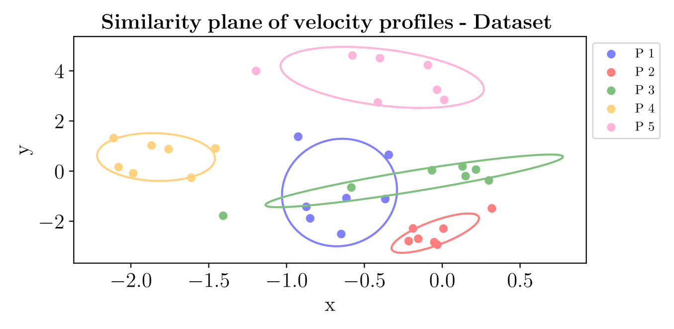
Figure 1: Similarity plane of velocity profiles for the dataset from [10]. Each color denotes the velocity profiles $\tilde{\nu}_{i}$ of a participant and the corresponding covariance ellipse.

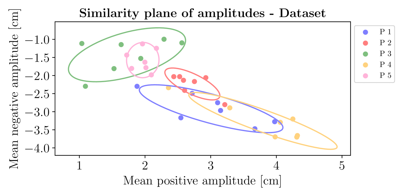
Figure 2: Similarity plane of amplitudes for the dataset from [10]. Each color denotes the amplitudes ($\bar{A}^{+}_{p}$, $\bar{A}^{-}_{p}$) of a participant and the corresponding covariance ellipse.

To quantify the similarity between individual motor signatures, we employ two metrics: overlap [18] and center distance.

Let $E_{i}\subset\mathbb{R}^{n_{\mathrm{d}}}$ denote the ellipse associated to individual $i$. The overlap $\Omega_{ij}\in[0,1]$ between the ellipses of individuals $i$ and $j$ is given by $\Omega_{ij}\coloneqq m_{L}(E_{i}\cap E_{j})/m_{L}(E_{i}\cup E_{j})$. A small $\Omega_{ij}$ indicates distinct motor behaviors, whereas a large $\Omega_{ij}$ suggests greater similarity between individuals. The center distance is defined as $\delta^{\mathrm{c}}_{ij}\coloneqq\left\lVert c_{i}-c_{j}\right\rVert_{2}$. In general, the smaller $\delta^{\mathrm{c}}_{ij}$ is, the more similar the IMSs of participants $i$ and $j$ are.

II-D Amplitude envelopes

Consider a scalar discrete-time signal $p:\mathcal{T}\to\mathbb{R}$, where $\mathcal{T}\subset\mathbb{Z}$ is finite. We define the velocity of $p$ as $v(t)\coloneqq(p(t)-p(t-1))/T_{\mathrm{s}}$, where $T_{\mathrm{s}}\in\mathbb{R}_{>0}$, and the first element of $v$ is $0$. We define the positive and negative amplitude envelopes, denoted by $A_{p}^{+},A_{p}^{-}:\mathbb{Z}\to\mathbb{R}$ respectively, as two signals, computed via the difference equations

$$A_{p}^{+}(t)=\begin{dcases}p(t),&\text{if }v(t)\leq 0,v(t-1)>0,p(t)>0,\\ A_{p}^{+}(t-1),&\text{otherwise},\end{dcases}$$

$$A_{p}^{-}(t)=\begin{dcases}p(t),&\text{if }v(t)\geq 0,v(t-1)<0,p(t)<0,\\ A_{p}^{-}(t-1),&\text{otherwise},\end{dcases}$$

with the first elements of $A_{p}^{+},A_{p}^{-}$ set to $0$. Then, we define the mean positive and negative amplitudes as

$$\bar{A}^{+}_{p}\coloneqq\frac{1}{\lvert\mathcal{T}\rvert}\sum_{t\in\mathcal{T}}A^{+}_{p}(t),\qquad\bar{A}^{-}_{p}\coloneqq\frac{1}{\lvert\mathcal{T}\rvert}\sum_{t\in\mathcal{T}}A^{-}_{p}(t).$$ (2)

III Data-driven model of human motion

To overcome the limitations of Kuramoto-like models in describing human motion, as observed in [11], we employ a fully data-driven approach using Long Short-Term Memory (LSTM) networks. LSTMs are a type of recurrent neural network capable of learning long-term dependencies in datasets, effectively addressing the vanishing gradient problem [21]. Specifically, we design a unified architecture and train a separate instance for each individual.

III-A Architecture of the generative model

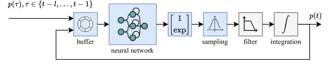
Figure 3: Schematic representation of the data-driven generative model of human motion described in Section III-A.

A graphical representation of the proposed architecture is shown in Figure 3. The model begins generating signals after a lookback window of time $l\in\mathbb{N}$. At each time instant $t>l$, the LSTM model receives the last $l$ position samples, $p(t-1),\dots,p(t-l)$, and outputs two values; an exponential is applied to the latter to ensure it is positive. These values are interpreted as the mean $\hat{\mu}(t)\in\mathbb{R}$ and standard deviation $\hat{\sigma}(t)\in\mathbb{R}_{\geq 0}$ of a Gaussian distribution, respectively. From this distribution, we sample a value $\hat{v}(t)\sim\mathcal{N}\left(\hat{\mu}(t),\hat{\sigma}(t)\right)$. This value is filtered using a first-order low-pass filter to obtain

$$\hat{v}^{\mathrm{f}}(t)=(1-\beta)\hat{v}^{\mathrm{f}}(t-1)+\beta\hat{v}(t),$$ (3)

where $\beta\in(0,1)$ is the filter gain. Then, a position sample is obtained as

$$\hat{x}(t)=\hat{x}(t-1)+T_{\mathrm{s}}\hat{v}^{\mathrm{f}}(t),$$ (4)

where $T_{\mathrm{s}}\in\mathbb{R}_{>0}$ is a sampling time. The new position sample $\hat{x}(t)$ is fed back into the input sequence (in an auto-regressive process), and the oldest is removed, maintaining an input window of length $l$. These steps are iterated to generate a signal of the desired duration.

III-B Dataset

To train our data-driven model, we use the dataset reported in  [10], which captures finger position as participants oscillate it back and forth along a line, at a preferred frequency. The data was captured through Leap Motion sensors [22] on the Chronos platform [23] (for more details on the experimental setup and protocol, see [10]). Since we aim to model individual motion in the absence of external influence, we focus on trials where participants moved without feedback from partners. The resulting dataset consists of $n_{\mathrm{s,p}}=7$ trials per participant, with $n_{\mathrm{p}}=5$ participants, yielding a total of $n_{\mathrm{s}}=35$ signals. Each time series lasts $30\,\text{s}$, was sampled at $10\,\text{Hz}$, interpolated via spline to $100\,\text{Hz}$, and processed with a Butterworth filter using a cutoff frequency twice the typical one associated with natural human movement ($\approx 3\,\text{Hz}$) [10].

The sampling time in (4) is chosen as $T_{\mathrm{s}}=0.01\,\text{s}$, to reflect that signals in the dataset are sampled at $100\,\text{Hz}$, while the gain in (3) is chosen as $\beta=60T_{\mathrm{s}}$ to guarantee a cut-off frequency that is at least $10$ times the typical frequency of human natural movement ($\approx 3\,\text{Hz}$). Hence, the set of time instants is $\mathcal{T}=\{1,\dots,3000\}$.

Name	Symbol	Value
LSTM
Number of LSTM cells per layer	$n_{\text{c}}$	$20$
Learning rate	$\alpha$	$10^{-4}$
Lookback window	$l$	$400$
Number of training epochs	$n_{\text{e}}$	$8000$
Number of epochs between model savings	$n^{\mathrm{s}}_{\mathrm{e}}$	$100$
Batch size	$n_{\mathrm{b}}$	$2000$
Dataset
Number of signals per person	$n_{\mathrm{s,p}}$	$7$
Signals for training and validation per person	$n_{\mathrm{tv}}$	$6$
Fraction of dataset for training	$d_{\%}$	$0.7$

TABLE I: Parameters used in the paper.

III-C Training of the LSTM network

In the remainder of this Section, we describe the training process for the data-driven model associated with any one of the $n_{\mathrm{p}}$ participants, omitting explicit notation of the individual considered, for the sake of readability.

The LSTM network is trained to predict the next value of the velocity signal, $v(t)=(p(t)-p(t-1))/T_{\mathrm{s}}$, given the input sequence $(p(t-l),\dots,p(t-1))$. Hence, the loss function to be minimized during the learning process is the negative log-likelihood between the target sample $v(t)$ and the estimated normal distribution $\mathcal{N}\left(\hat{\mu}(t),\hat{\sigma}(t)\right)$ (see, e.g., [15]). As the estimated distribution is Gaussian, the loss function takes the form [24]

$$L=\frac{1}{2}\left(\log\left(\hat{\sigma}^{2}(t)\right)+\frac{\left(\hat{\mu}(t)-v(t)\right)^{2}}{\hat{\sigma}^{2}(t)}\right).$$ (5)

The final loss is computed as the average of the value of (5) over a batch of $n_{\mathrm{b}}$ samples.

For each person in the dataset, a separate model is trained. Namely, $n_{\mathrm{tv}}$ out of $n_{\mathrm{s,p}}$ signals (of each person) are used to train the corresponding model, with training performed over $n_{\mathrm{e}}$ epochs. A fraction $d_{\%}$ of each of the $n_{\mathrm{tv}}$ signals is allocated for training, while the remaining portion is used for validation.

The neural network consistes of $2$ LSTM layers followed by a fully connected layer with linear activation function. The learning rate $\alpha$ and other parameters are listed in Table I. Training is performed using the Adam optimization algorithm. The architecture is implemented in Python, via the PyTorch library [25].

III-D Model selection and validation

During the training described in Section III-C, network weights are saved every $n^{\mathrm{s}}_{\mathrm{e}}$ epochs and are denoted as $w_{\mathrm{h}}$, where $h\in\{1,\dots,\lfloor n_{\mathrm{e}}/n_{\mathrm{e}}^{\mathrm{s}}\rfloor\}$. For each $h$, we use the data-driven model to generate $n_{\mathrm{s,p}}$ new position signals, denoted as $p_{i}^{\mathrm{g},h}:\mathcal{T}\to\mathbb{R}$ for $i\in\{1,\dots,n_{\mathrm{s,p}}\}$, using the corresponding weights set $w_{\mathrm{h}}$, and setting $p_{i}^{\mathrm{g},h}(t)=p_{i}^{\mathrm{d}}(t)$ for $t\in\{1,\dots,l\}$ (see, e.g., Figure 4), where $p_{i}^{\mathrm{d}}(t):\mathcal{T}\to\mathbb{R}$ is a signal from the dataset. We denote by $\nu^{\mathrm{d}}_{i}$ and $\nu^{\mathrm{g},h}_{i}$, for $i\in\{1,\dots,n_{\mathrm{s,p}}\}$, the velocity profiles obtained from the signals in the dataset and those generated by the data-driven model, respectively. Next, we compute two key quantities. The first is the mean EMD between the velocity profiles of the generated signals and those of dataset signals:

$$\bar{e}_{\mathrm{\nu}}^{h}=\frac{1}{n_{\mathrm{s,p}}}\sum_{i=1}^{n_{\mathrm{s,p}}}\delta^{\mathrm{em}}\left(\nu^{\mathrm{d}}_{i},\nu^{\mathrm{g},h}_{i}\right).$$

The second is the root mean squared amplitude error

$$\bar{e}_{A}^{h}=\sqrt{\begin{aligned} &\left(\frac{1}{n_{\mathrm{s,p}}}\sum_{i=1}^{n_{\mathrm{s,p}}}\frac{1}{|\mathcal{T}|}\sum_{t\in\mathcal{T}}\left\lvert A^{+}_{p_{i}^{\mathrm{d}}}(t)-A^{+}_{p_{i}^{\mathrm{g},h}}(t)\right\rvert\right)^{2}\\ &+\left(\frac{1}{n_{\mathrm{s,p}}}\sum_{i=1}^{n_{\mathrm{s,p}}}\frac{1}{|\mathcal{T}|}\sum_{t\in\mathcal{T}}\left\lvert A^{-}_{p_{i}^{\mathrm{d}}}(t)-A^{-}_{p_{i}^{\mathrm{g},h}}(t)\right\rvert\right)^{2}\end{aligned}}.$$

Then, we define the cost function

$$J^{h}\coloneqq q_{\nu}\left(\frac{\bar{e}_{\mathrm{\nu}}^{h}}{\max_{h}\bar{e}_{\mathrm{\nu}}^{h}}\right)^{2}+q_{A}\left(\frac{\bar{e}_{\mathrm{A}}^{h}}{\max_{h}{\bar{e}_{\mathrm{A}}^{h}}}\right)^{2},$$

where, $q_{\nu},q_{A}\in\mathbb{R}_{\geq 0}$ are importance weights. We set $q_{\nu}=100$, $q_{A}=0.01$. The final set of network weights is selected as $w^{\star}=\arg\min_{h}J^{h}$.

IV Results

IV-A Individual motor signature characterization via motion amplitude

Individual motor signatures are typically characterized using velocity profiles [18]. However, in this study, we introduce the use of mean positive and negative amplitudes (see (2)) as a novel approach to describing individual motor characteristics. Figure 2 illustrate the values of $\bar{A}^{+}_{p}$ and $\bar{A}^{-}_{p}$ for each participants across various trials, effectively mapping a similarity plane for motion amplitudes. Notably, after generating ellipses as described in Section II-C, we observe that the ellipses associated to different individuals remain relatively distinct, suggesting that amplitude-based features can effectively capture individual differences in motor behavior. In general, identifying decent features for characterizing individual motor signatures is not straightforward. Indeed, attempts at doing so via spectral content and acceleration profiles did not yield clearly separated ellipses (results omitted for brevity), reinforcing the potential of amplitude-based features for motor signature characterization.

IV-B Signal generation

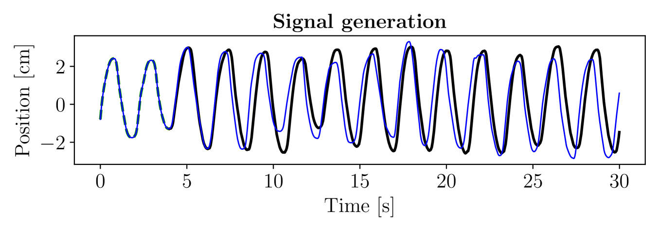
Figure 4: Generation of a motion signal for participant 2. The blue line is the recorded signal; the green dashed line is the segment given as input to the data-driven model; the black line is the generated signal.

To qualitatively assess the generative performance of the data-driven model designed in Section III-A, in Figure 4, we compare a representative position signal recorded for a specific person with the signal generated by the data-driven model identified for that individual, when the model is fed with the former signal, for the first $l$ time instants. The generated signal consistently maintains a shape similar to the recorded signal, indicating the model’s ability to capture the person’s motion signature. However, the generated signal is not identical to the recorded one, highlighting the model’s capability to produce original motion.

IV-C Similarity analysis

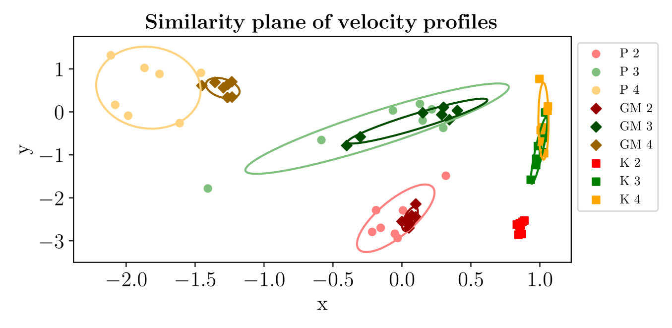
Figure 5: Similarity plane of velocity profiles for representative participants (P). “GM $i$” denotes profiles obtained by the generative model trained after participant $i$; “K $i$” denotes profiles obtained through a Kuramoto oscillator tuned after participant $i$.

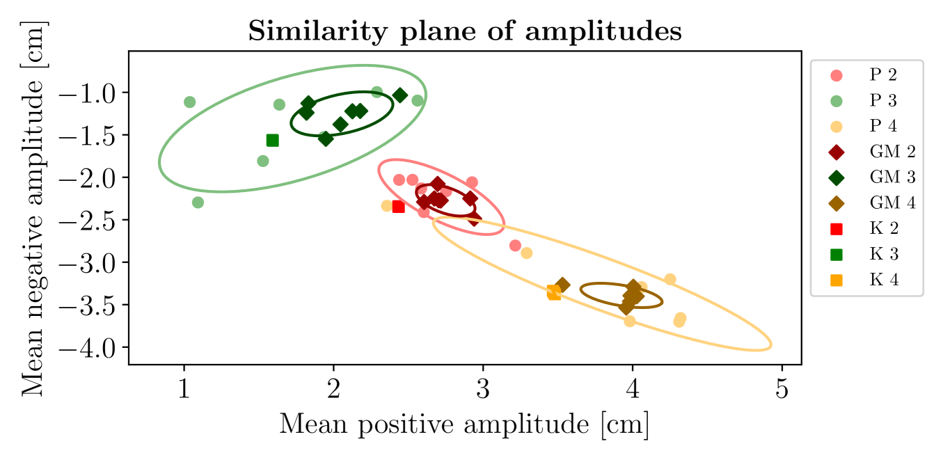
Figure 6: Similarity plane of amplitudes for representative participants (P). “GM $i$” denotes amplitudes obtained by the generative model trained after participant $i$; “K $i$” denotes amplitudes obtained through a Kuramoto oscillator tuned after participant $i$ (each appears as a single point as all associated position signals share the same amplitude).

To quantify the modeling accuracy of the data-driven models, we use the similarity metrics introduced in Section II-C. In Figures 5, 6, we show the similarity planes of velocity profiles and amplitudes, respectively, comparing ellipses obtained by the participants with those obtained from our generative model. We observe that the ellipses of the generative model are typically well contained in the ellipses of the corresponding participant, and the main axis of the ellipses are also aligned, indicating a good capability of the model to behave similarly to the person it was trained after.

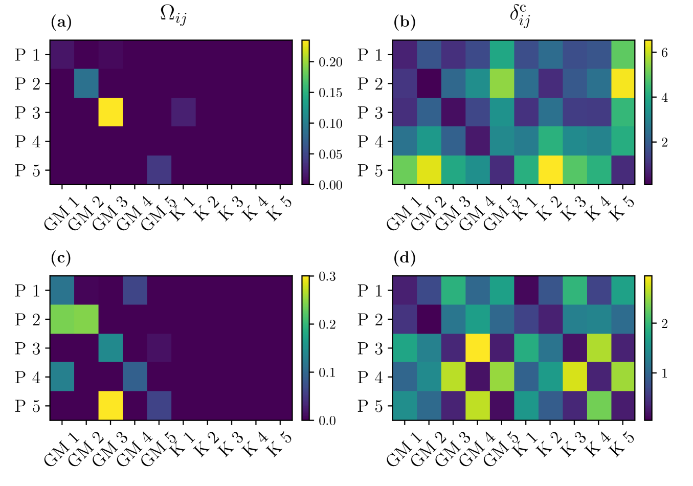
Figure 7: Heatmaps of two metrics in two spaces. (a) Overlaps $\Omega_{ij}$ (higher is better) and (b) center distances $\delta^{\mathrm{c}}_{ij}$ (lower is better) in similarity space of velocity profiles; (c) Overlaps and (d) center distances in similarity space of amplitudes.

In Figure 7, we report the overlaps $\Omega_{ij}$ and the center distances $\delta^{\mathrm{c}}_{ij}$ (see Section II-C) computed comparing the ellipses of the generative models against those of the participants. The overlap tends to be significantly larger, and the center distance smaller, when the model trained to mimic a certain participant is compared with that same participant rather than with others. This confirms that the generative models effectively capture individual motion characteristics while remaining distinct from one another.

IV-D Comparison with state-of-the-art models

Next, we compare the capability to imitate human IMS of our generative models against those of fixed-frequency Kuramoto oscillators (similar to those used in [7, 9, 10]). The position signals generated by these oscillators are given by $x_{\mathrm{K}}(t)=A_{\mathrm{K}}\sin(\omega_{\mathrm{K}}t)$, where, for each participant, $\omega_{\mathrm{K}}$ is sampled at each trial from a Gaussian distribution with mean and variance taken from [10]. The amplitude $A_{\mathrm{K}}$ is fixed for each trial and is computed, for each individual, as $A_{\mathrm{K}}=\frac{\bar{A}^{+}+\left|\bar{A}^{-}\right|}{2}$, where $\bar{A}^{+}=\frac{1}{n_{\mathrm{s,p}}}\sum_{i=1}^{{n_{\mathrm{s,p}}}}\bar{A}^{+}_{p^{\mathrm{d}}_{i}}$ and $\bar{A}^{-}=\frac{1}{n_{\mathrm{s,p}}}\sum_{i=1}^{{n_{\mathrm{s,p}}}}\bar{A}^{-}_{p^{\mathrm{d}}_{i}}$ (considering the position signals $p^{\mathrm{d}}_{i}$ associated to that individual). From such position signals, we extract velocity profiles and amplitudes to generate similarity planes and covariance ellipses to be compared with those of the participants.

In Figures 5, we observe that the covariance ellipses of the velocity profiles generated by Kuramoto oscillators are entirely different from those generated by the participants. This is also confirmed in Figure 8, portraying representative velocity profiles: while those of the participant and the generative model are qualitatively similar, that of the Kuramoto oscillator is remarkably different. In Figure 6, depicting the similarity plane of amplitudes, we see that the ellipses for Kuramoto oscillators have null measure, resulting in poor overlap value. The superior imitation performance of the generative model, compared to the Kuramoto oscillators, is confirmed by Figure 7 detailing the similarity metrics for all cases.

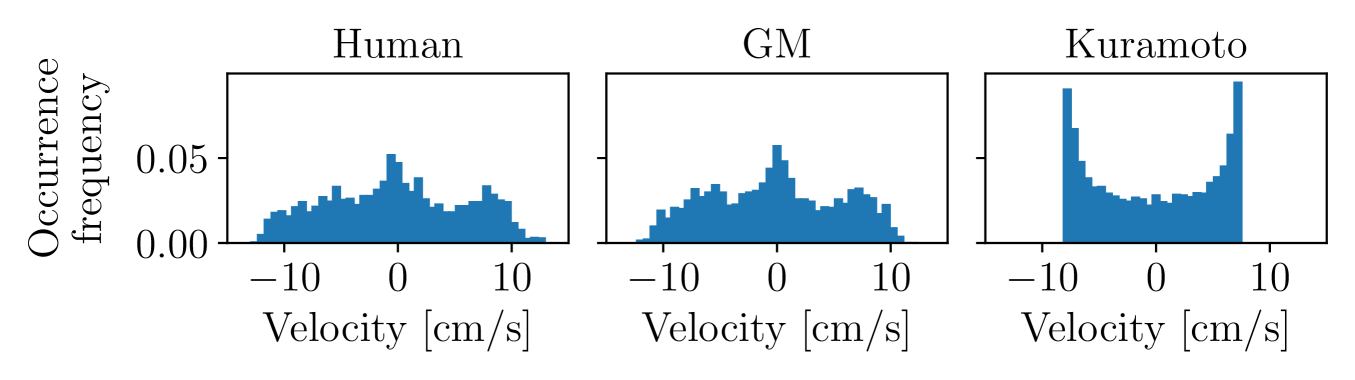
Figure 8: Comparison of velocity profiles for a representative motion between a participant, our generative model (GM) and a Kuramoto oscillator.

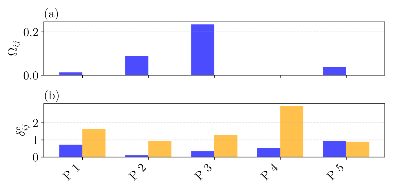
Figure 9: Comparison between the data-driven generative model (blue) and the Kuramoto oscillator (orange) in reproducing the individual motor signatures of different participants (P) as described by their velocity profiles.

A more direct comparison is offered in Figure 9, where we report the similarity metrics obtained by the generative model and the Kuramoto oscillators when attempting to replicate the velocity profiles of the participants. Again, we observe significantly better performance for the generative models (higher $\Omega_{ij}$, lower $\delta_{ij}^{\mathrm{c}}$) than for the fixed-frequency oscillators.

V Conclusion

Modeling human motion behavior is essential for designing artificial avatars and robots that collaborate with people in motor tasks. However, existing models rely on overly simplistic assumptions that do not hold in practice, hindering the development of advanced cognitive architectures to drive such artificial agents.

In this work, we have proposed a data-driven approach to modeling human motion behavior. Our model exploits a LSTM network to learn how to predict the distributions of future velocity samples starting from position timeseries. After showing the validity of amplitudes of motion as descriptors of individual motor signatures, we use various metrics to convincingly show that our generative model, opportunely trained, can capture the behavioral peculiarities of individuals performing an oscillatory motor task. In addition, our model significantly outperforms state-of-the-art fixed-frequency oscillators at reproducing human motor behavior.

Future work includes extending the proposed generative model to add response to external stimuli, to assemble networks of interacting generative models.

References

- [1] G. C. Homans, The human group. Routledge, 2017.
- [2] M. Rennung and A. S. Göritz, “Prosocial consequences of interpersonal synchrony,” Zeitschrift für Psychologie, 2016.
- [3] M. C. Howard, “A meta-analysis and systematic literature review of virtual reality rehabilitation programs,” Computers in Human Behavior, vol. 70, pp. 317–327, 2017.
- [4] D. L. Neumann, R. L. Moffitt, P. R. Thomas, K. Loveday, D. P. Watling, C. L. Lombard, S. Antonova, and M. A. Tremeer, “A systematic review of the application of interactive virtual reality to sport,” Virtual Reality, vol. 22, pp. 183–198, 2018.
- [5] P. Langley, J. E. Laird, and S. Rogers, “Cognitive architectures: Research issues and challenges,” Cognitive Systems Research, vol. 10, no. 2, pp. 141–160, 2009.
- [6] L. Noy, E. Dekel, and U. Alon, “The mirror game as a paradigm for studying the dynamics of two people improvising motion together,” Proceedings of the National Academy of Sciences, vol. 108, no. 52, pp. 20947–20952, 2011.
- [7] F. Alderisio, G. Fiore, R. N. Salesse, B. G. Bardy, and M. d. Bernardo, “Interaction patterns and individual dynamics shape the way we move in synchrony,” Scientific reports, vol. 7, no. 1, p. 6846, 2017.
- [8] Y. Kuramoto, “Self-entrainment of a population of coupled non-linear oscillators,” in International Symposium on Mathematical Problems in Theoretical Physics (H. Araki, ed.), (Berlin, Heidelberg), pp. 420–422, Springer Berlin Heidelberg, 1975.
- [9] S. Shahal, A. Wurzberg, I. Sibony, H. Duadi, E. Shniderman, D. Weymouth, N. Davidson, and M. Fridman, “Synchronization of complex human networks,” Nature communications, vol. 11, no. 1, p. 3854, 2020.
- [10] C. Calabrese, B. G. Bardy, P. De Lellis, and M. di Bernardo, “Modeling frequency reduction in human groups performing a joint oscillatory task,” Frontiers in Psychology, vol. 12, 2022.
- [11] A. Grotta, M. Coraggio, A. Spallone, F. De Lellis, and M. di Bernardo, “Learning-based cognitive architecture for enhancing coordination in human groups,” IFAC-PapersOnLine, vol. 58, no. 30, pp. 37–42, 2024.
- [12] Y. Wang, “A new concept using LSTM neural networks for dynamic system identification,” in 2017 American Control Conference (ACC), pp. 5324–5329, IEEE, 2017.
- [13] M. Aguiar, A. Das, and K. H. Johansson, “Universal approximation of flows of control systems by recurrent neural networks,” in 2023 62nd IEEE Conference on Decision and Control (CDC), pp. 2320–2327, 2023.
- [14] K. Fragkiadaki, S. Levine, P. Felsen, and J. Malik, “Recurrent network models for human dynamics,” in Proceedings of the IEEE International Conference on Computer Vision, pp. 4346–4354, 2015.
- [15] A. Alahi, K. Goel, V. Ramanathan, A. Robicquet, L. Fei-Fei, and S. Savarese, “Social LSTM: Human trajectory prediction in crowded spaces,” in 2016 IEEE Conference on Computer Vision and Pattern Recognition (CVPR), pp. 961–971, 2016.
- [16] N. Bisagno, B. Zhang, and N. Conci, “Group LSTM: Group trajectory prediction in crowded scenarios,” in Proceedings of the European Conference on Computer Vision (ECCV) Workshops, September 2018.
- [17] A. Graves, “Generating sequences with recurrent neural networks,” arXiv preprint arXiv:1308.0850, 2013.
- [18] P. Słowiński, C. Zhai, F. Alderisio, R. Salesse, M. Gueugnon, L. Marin, B. G. Bardy, M. Di Bernardo, and K. Tsaneva-Atanasova, “Dynamic similarity promotes interpersonal coordination in joint action,” Journal of The Royal Society Interface, vol. 13, no. 116, p. 20151093, 2016.
- [19] F. Santambrogio, Optimal Transport for Applied Mathematicians. Calculus of Variations, PDEs and Modeling, vol. 87. Springer, 2015.
- [20] I. Borg and P. J. Groenen, Modern multidimensional scaling: Theory and applications. Springer Science & Business Media, 2007.
- [21] S. Hochreiter and J. Schmidhuber, “Long short-term memory,” Neural Computation, vol. 9, pp. 1735–1780, 11 1997.
- [22] J. Guna, G. Jakus, M. Pogačnik, S. Tomažič, and J. Sodnik, “An analysis of the precision and reliability of the leap motion sensor and its suitability for static and dynamic tracking,” Sensors, vol. 14, no. 2, pp. 3702–3720, 2014.
- [23] F. Alderisio, M. Lombardi, G. Fiore, and M. di Bernardo, “A novel computer-based set-up to study movement coordination in human ensembles,” Frontiers in Psychology, vol. 8, 2017.
- [24] D. Nix and A. Weigend, “Estimating the mean and variance of the target probability distribution,” in Proceedings of 1994 IEEE International Conference on Neural Networks (ICNN’94), vol. 1, pp. 55–60 vol.1, 1994.
- [25] A. Paszke et al., “Pytorch: An imperative style, high-performance deep learning library,” arXiv preprint arXiv:1912.01703, 2019.