Prototype Perturbation for Relaxing Alignment Constraints in Backward-Compatible Learning

Abstract

The traditional paradigm to update retrieval models requires re-computing the embeddings of the gallery data, a time-consuming and computationally intensive process known as backfilling. To circumvent backfilling, Backward-Compatible Learning (BCL) has been widely explored, which aims to train a new model compatible with the old one. Many previous works focus on effectively aligning the embeddings of the new model with those of the old one to enhance the backward-compatibility. Nevertheless, such strong alignment constraints would compromise the discriminative ability of the new model, particularly when different classes are closely clustered and hard to distinguish in the old feature space. To address this issue, we propose to relax the constraints by introducing perturbations to the old feature prototypes. This allows us to align the new feature space with a pseudo-old feature space defined by these perturbed prototypes, thereby preserving the discriminative ability of the new model in backward-compatible learning. We have developed two approaches for calculating the perturbations: Neighbor-Driven Prototype Perturbation (NDPP) and Optimization-Driven Prototype Perturbation (ODPP). Particularly, they take into account the feature distributions of not only the old but also the new models to obtain proper perturbations along with new model updating. Extensive experiments on the landmark and commodity datasets demonstrate that our approaches perform favorably against state-of-the-art BCL algorithms.

I Introduction

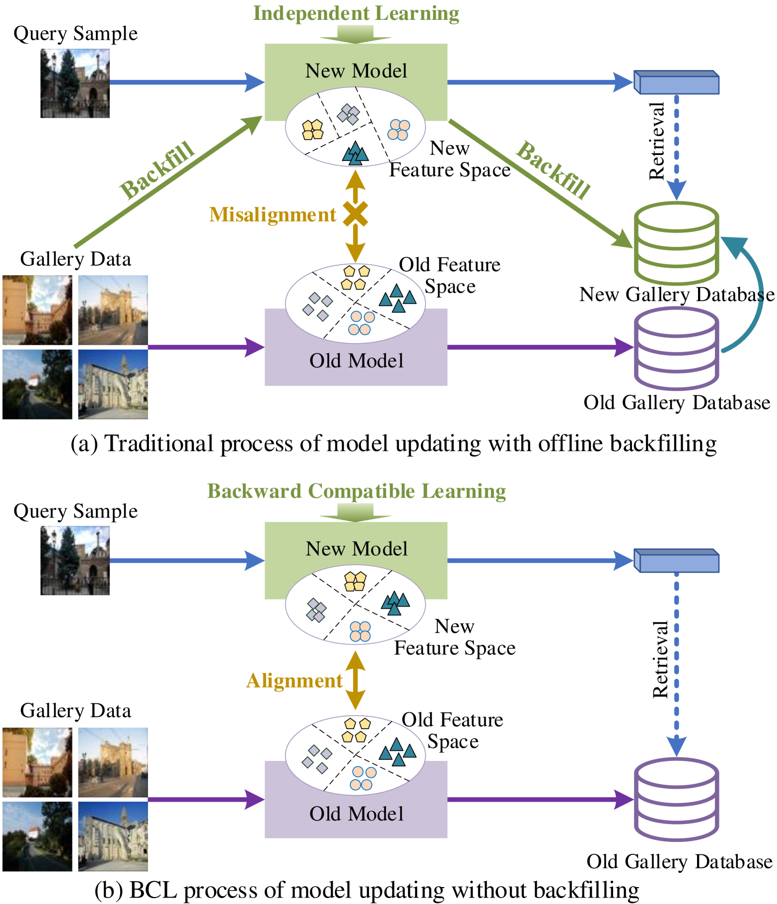
Figure 1: Two different paradigms for updating the embedding model for the retrieval system. (a) The new model is trained independently and used to re-extract the embeddings of all gallery data, i.e., backfilling, which is time-consuming and computationally intensive. (b) With backward-compatible learning, the query embedding is directly comparable with the existing gallery embeddings without backfilling.

Image retrieval has drawn much attention due to its wide range of applications [1, 2, 3, 4], such as E-commerce search and landmark localization. The retrieval systems typically employ an embedding model to transform raw data into high-dimensional vectors and maintain a large-scale gallery database storing the embeddings of the gallery data. Upon receiving a query sample, the online server calculates its embedding vector and compares the embedding with those in the gallery database to retrieve the most similar entries. As new training data or advanced model designs become available, retrieval service providers often desire to train a new model for better performance. However, if the new model is trained independently, its feature space naturally misaligns with that of the old one [5], being incompatible with existing gallery embeddings. Hence, the system needs to re-extract the embeddings of the gallery data with the new model, a process named “backfilling”, as shown in Figure 1 (a). Nevertheless, backfilling is time-consuming and computationally intensive for large-scale galleries.

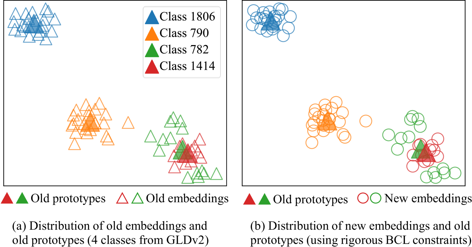
Figure 2: Distribution of the embeddings and prototypes of 4 classes from GLDv2 [6], which is visualized with t-SNE [7]. (a) Classes 782 & 1414 are nearly indistinguishable in the old feature space. (b) The new model is trained with rigorous alignment constraints to the old feature space, producing new embeddings strictly surrounding the old prototypes. As a result, the new embeddings of these classes are clustered closely and hard to distinguish.

To address this problem, Shen et al. [8] propose the Backward-Compatible Learning (BCL) methodology; it enables the new model to produce embeddings comparable with existing gallery embeddings, allowing for model updating without backfilling, as shown in Figure 1 (b). To be specific, Shen et al. [8] use the classifier of the old model to regularize the new model during training to achieve backward-compatibility. Subsequent studies further explore more sophisticated BCL methods. For example, LCE [9] and UniBCT [10] replace the softmax loss with ArcFace loss [11] to regularize the new model. AdvBCT [5] integrates adversarial learning into new model training, coupled with an elastic boundary mechanism to constrain the distribution of new embeddings.

Most of the aforementioned methods essentially enforce the embeddings of the new model to strictly align with those of the old model to enhance the backward-compatibility. Despite the impressive performance, they pay less attention to the potential adverse effect of the old feature distribution on the new model during BCL, which may hurt the discriminative ability of the new model. For instance, if two different classes are distributed closely and become nearly indistinguishable in the old feature space, imposing strict alignment constraints between the new and old models would cause these classes to remain indistinguishable in the new feature space. Figure 6 (a) and (b) illustrate such a case, where the new embeddings of Classes 782 & 1414 become indistinguishable due to the overstrict alignment constraints.

To alleviate the adverse effect of the indistinguishable classes in the old feature space, we propose introducing perturbations to the old feature space, enabling backward-compatible learning with a more flexible alignment constraint. Given that individual sample features may be noisy in representing the feature distribution, we opt to apply perturbations to the old class centers, i.e., old prototypes, which are robust to outliers. Technically, we impose perturbations to old prototypes to adaptively move them away from their indistinguishable neighbors, as shown in Figure 3 (a). Then, we can constrain the new feature space to align with the pseudo-old feature space characterized by the perturbed old prototypes, learning a new model with strong discriminative ability. The core challenge of this idea lies in determining appropriate directions and amplitudes for the perturbations to enhance the discriminative ability of the new model without compromising its backward-compatibility.

In this paper, we devise two implementations for prototype perturbation: Neighbor-Driven Prototype Perturbation (NDPP) and Optimization-Driven Prototype Perturbation (ODPP), which both calculate perturbations based on the similarities between prototypes. NDPP employs a heuristic approach to calculate the perturbation for an old prototype based on the repulsion from its neighboring prototypes, while ODPP learns the perturbations for old prototypes by optimizing an objective function designed to push similar prototypes away from each other. Notably, NDPP and ODPP leverage the prototypes of not only the old model but also the new model to determine the perturbations during BCL. This design allows for continual adjustment of perturbations conditioned on the new feature space, producing more suitable perturbations to enhance the discriminative ability of the new model. We conduct extensive experiments on the landmark [6, 12] and commodity [13] datasets. The experimental results demonstrate that NDPP and ODPP both substantially improve the retrieval performance of the new model without compromising the cross-model retrieval performance. Our contributions are summarized as follows:

• We propose a prototype perturbation mechanism to adaptively relax the alignment constraints for BCL to enhance the discriminative ability of the new model.

• We develop two novel approaches, neighbor-driven prototype perturbation and optimization-driven prototype perturbation, to implement the prototype perturbation mechanism; they leverage both the old and new prototypes to produce effective perturbations for robust BCL.

• Extensive experiments on diverse datasets demonstrate that both NDPP and ODPP perform favorably against state-of-the-art BCL methods, which showcases the effectiveness of our prototype perturbation mechanism.

II Related Work

Backward-compatible learning. To avoid backfilling for retrieval model updating, Shen et al. [8] propose the backward-compatible learning method to train a new embedding model compatible with the old one. It regularizes the new model with the classifier of the old model. Afterward, many algorithms [9, 14, 15, 16, 17, 18, 19] have been proposed to improve BCL performance. Several of them resort to contrastive learning [20]. For example, Duel-tuning [14] designs a prototype-based contrastive loss to align the new embeddings with the old prototypes. RACT [15] and RM [21] use a contrastive loss to leverage both positive and negative samples. Besides contrastive learning, other sophisticated compatible learning mechanisms are also explored. AdvBCT [5] employs an elastic boundary to constrain the new embeddings and introduces adversarial learning to minimize the distribution disparity between new and old embeddings. $\text{BT}^{2}$ [16] extends the representation of the new model with extra dimensions and proposes a basis transformation for BCL. SSPL [22] designs a structure similarity preserving method to achieve feature compatibility between the query model and gallery model. RBCL [23] proposes a ranking-based BCL method that directly optimizes the ranking metric between new and old features. LCE [9] and UniBCT [10] use the ArcFace loss [11] to regularize the new model to achieve backward-compatibility.

Notably, UniBCT [10] designs a structural prototype refinement method to alleviate the effects of outlier samples on prototype calculation by propagating the knowledge within neighboring intra-class samples. Unlike UniBCT, which focuses only on the intra-class samples for each prototype, our method constructs a more distinguishable pseudo-old feature space by perturbing the prototypes of different classes over the entire feature space.

Compatible learning with backfilling. Besides backward-compatible learning, several works [24, 15, 21, 25, 26] also explored how to perform backfilling more efficiently. Specifically, FCT [24] introduces a forward-compatible framework to map old embeddings to the new feature space, which however relies on side information from an additional model. RACT [15] deploys the new model immediately after the model upgrade and performs backfilling online to improve the performance gradually. BiCT [25] leverages a forward-compatible module to transform the old gallery embeddings into new feature space for better performance. RM [21] proposes an online backfilling approach based on distance rank merge and incorporates a reverse query transform module to achieve a more efficient merging process. FastFill [27] measures the quality of gallery features with an alignment loss and backfills the feature with the poorest quality first. DMU [26] performs selective backward-compatible learning along with a forward adaption, assigning larger backward-compatible weights to the old features with better discriminativeness, and larger adaption degree in the forward adaptive loss to those with poorer discriminativeness.

Lifelong learning. Lifelong learning [28, 29, 30, 31], also known as continuous learning, aims to learn new knowledge from continuously collected data without forgetting the previously learned knowledge. Most of the lifelong learning algorithms are typically designed to update their model incrementally in response to incoming data and tasks without considering the interaction within the different models, i.e., the updated model is not compatible with the old one. Several continuous learning algorithms [32, 33] propose to augment and replay the prototype of previous tasks to alleviate the catastrophic forgetting problem. The augmented prototypes in these methods are used to maintain the decision boundary of previous tasks, while the perturbations on prototypes in our algorithm aim to alleviate the impact of the old inaccurate discriminative boundary. Besides, several recent studies [34, 35] explore the lifelong person re-identification methods with backward-compatibility. Similar to existing BCL methods, these two methods also impose strict alignment constraints between the new and old feature spaces.

Contrastive learning. In recent years, contrastive learning [36, 37, 38, 39, 40, 41] has emerged as a powerful paradigm for unsupervised representation learning, achieving remarkable performance improvements. For instance, SimCLR [37] applies various data augmentations and maximizes the agreement between different augmented views of the same image. Moco V1 [36] trains a visual representation encoder by leveraging a momentum-based contrastive loss. Contrastive learning is widely applied in retrieval [42, 43, 44] and backward-compatible learning [14]. Several algorithms [14, 15, 21] have investigated the point-to-point (P2P) contrastive learning and point-to-set (P2S) contrastive learning methods for BCL. The former is vulnerable to the outlier samples, while the latter dilutes the influence of the individual outlier sample by computing the average among a set. We use the P2S contrastive learning method as the baseline to develop our backward-compatible learning algorithms.

III Methodology

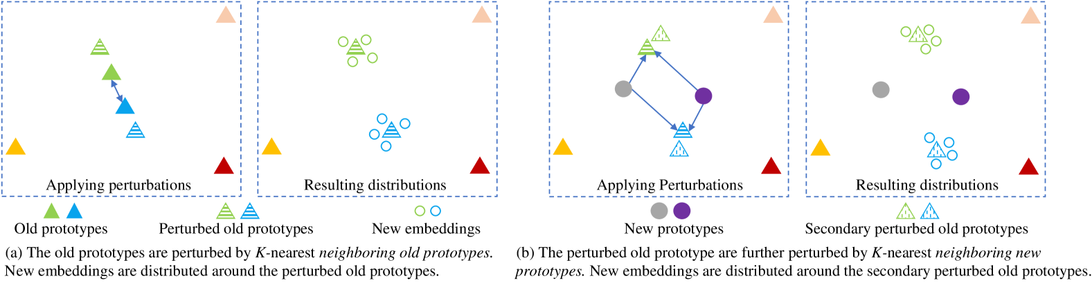
Figure 3: Illustration of neighbor-driven prototype perturbation. (a) Perturbations are calculated based on the neighboring old prototypes, and new embeddings are constrained to align with the perturbed old prototypes. (b) Perturbations are updated based on the neighboring new prototypes, and new embeddings are constrained to align with the secondary perturbed old prototypes.

III-A Preliminaries

Problem formulation. Backward-Compatible Learning (BCL) aims to acquire a new embedding model compatible with the frozen old one. Denote the old and new models as $\phi_{o}\!\!:\!\!x\!\!\xrightarrow{}\!\!\mathbb{R}^{D_{o}}$ and $\phi_{n}\!\!:\!\!x\!\!\xrightarrow{}\!\!\mathbb{R}^{D_{n}}$, where $D_{o}$ and $D_{n}$ represent the dimensions of old and new embeddings, and $\phi_{o}$ and $\phi_{n}$ are trained on the datasets $\mathcal{T}_{o}$ and $\mathcal{T}_{n}$, respectively. Typically, $\mathcal{T}_{o}$ can be a subset of $\mathcal{T}_{n}$. Suppose we have a retrieval performance evaluation metric $\mathcal{M}(\phi_{q},\phi_{g},\mathcal{Q},\mathcal{G})$, where $\mathcal{Q}$ and $\mathcal{G}$ are the query and gallery sets, and $\phi_{q}$ and $\phi_{g}$ are the models used to extract the embeddings of $\mathcal{Q}$ and $\mathcal{G}$, respectively. The new model $\phi_{n}$ is recognized to be backward-compatible with $\phi_{o}$ if it satisfies the empirical criterion $\mathcal{M}(\phi_{n},\phi_{o},\mathcal{Q},\mathcal{G})\!>\!\mathcal{M}(\phi_{o},\phi_{o},\mathcal{Q},\mathcal{G})$ [8]. To this end, a robust new-to-old distance metric satisfying the following inequality is necessary [17]:

$$\begin{split}&d(\phi_{n}(x_{i}),\phi_{o}(x_{j}))<d(\phi_{n}(x_{i}),\phi_{o}(x_{k})),\\ &{\forall}(i,j,k)\in\{(i,j,k):y_{i}=y_{j}\neq y_{k}\}.\end{split}$$ (1)

Herein $y_{i}$, $y_{j}$, and $y_{k}$ are the labels for samples $x_{i}$, $x_{j}$, and $x_{k}$, respectively. $d(\cdot,\cdot)$ denotes the distance metric.

Besides the backward-compatibility, the discriminative ability of the new model is also crucial for BCL, which is usually evaluated by comparing its retrieval performance with that of a new model trained independently.

Prototype-based contrastive learning for BCL. Contrastive learning is typically introduced to learn a robust new-to-old distance metric in BCL, including the point-to-point (P2P) [15, 21] and point-to-set (P2S) [14] contrastive learning methods. The P2P method tends to be sensitive to outliers in the old feature space. In contrast, the P2S method considers a set of samples from the same class as positive or negative examples. The influence of the individual outlier sample is diluted by the sample set, and thus P2S contrastive learning deals with the outliers more robustly. Hence, we prefer P2S contrastive learning as our baseline method.

We perform P2S contrastive learning with the prototype of each class, which is the average of the embeddings belonging to that class, i.e., the class center. During BCL, we use the frozen old model to extract the embeddings of samples in $\mathcal{T}_{n}$ and then compute the prototypes of all classes. They together represent the feature distribution of the old model and are referred to as old prototypes. Denoting the old prototype of class $c$ by $p_{o}^{c}$, the prototype-based contrastive loss for training the new model $\phi_{n}$ can be formulated as:

$$\mathcal{L}_{bc}=-\log\frac{{\exp(\langle e_{n}^{c},p^{c}_{o}\rangle/\tau)}}{{\sum_{{c^{\prime}\in\mathcal{C}}}\exp(\langle e_{n}^{c},p^{c^{\prime}}_{o}\rangle/\tau)}},$$ (2)

where $\langle\cdot,\cdot\rangle$ denotes cosine similarity, $e_{n}^{c}=\phi_{n}(x^{c})$, $x^{c}\!\in\!\mathcal{T}_{n}$ is the sample belonging to class $c$, $\mathcal{C}$ is the class set of $\mathcal{T}_{n}$, and $\tau$ is the temperature factor.

Following existing approaches [8, 5], we formulate the discriminative learning of the new model as a classification task. Specifically, we build a fully connected layer on the embedding model and introduce a cross-entropy loss $\mathcal{L}_{ce}$ for classification. Hence, the overall training objective of the new model can be formulated as:

$$\mathcal{L}=\mathcal{L}_{ce}+\lambda\mathcal{L}_{bc}.$$ (3)

Herein $\lambda$ is a balance weight for $\mathcal{L}_{bc}$.

III-B Overview of prototype perturbation

Although prototype-based contrastive learning addresses the outlier issue, it still suffers from the adverse effect of the indistinguishable classes in the old feature space, due to the strict alignment constraint formulated by Eq. (2). To alleviate this adverse effect, we propose the prototype perturbation mechanism to generate a pseudo-old feature distribution as the backward-compatible learning target. Although the new embeddings are constrained to surround the pseudo-old prototypes, Eq. (1) can still be satisfied as long as the perturbation is appropriately determined. Technically, the key to prototype perturbation is how to properly push the old prototypes away from their indistinguishable neighbors.

In light of this idea, we devise two approaches to determine the perturbations: Neighbor-Driven Prototype Perturbation (NDPP) and Optimization-Driven Prototype Perturbation (ODPP). NDPP and ODPP will produce the pseudo-old prototypes for calculating the prototype-based contrastive loss. Namely, our two approaches will update Eq. (2) to improve the backward-compatible learning performance. In the following, we detail the NDPP and ODPP approaches and present how to leverage the pseudo-old prototypes to perform backward-compatible learning.

III-C Neighbor-driven prototype perturbation

NDPP calculates the perturbation for an old prototype based on its similarity with the neighbors. The basic principle is that each old prototype is presumed to experience repulsion from its neighbors, and the intensity of the repulsion is proportional to their similarity. Specifically, we consider the neighbors from both the old and new feature spaces for each old prototype to be perturbed. Next, we present the prototype perturbation based on different neighbors.

Prototype perturbation based on old neighbors. Figure 3 (a) illustrates the prototype perturbation scheme based on old neighboring prototypes. For the old prototype $p^{c}_{o}$ of class $c$, we first find its $K$-nearest neighbors by calculating its cosine similarities with the old prototypes of the other classes. We denote the $K$-nearest neighbors by $\{p_{o}^{c^{\prime}}\}_{c^{\prime}\in\mathcal{K}_{o}^{c}}$ and the corresponding similarities by $\{s_{o2o}^{c^{\prime}}\}_{c^{\prime}\in\mathcal{K}_{o}^{c}}$, where $\mathcal{K}_{o}^{c}$ denotes the class set of these neighbors. We calculate the perturbation $r^{c}_{o}$ for the old prototype $p_{o}^{c}$ by:

$$r^{c}_{o}=\frac{\sum_{c^{\prime}\in\mathcal{K}_{o}^{c}}s_{o2o}^{c^{\prime}}(p^{c}_{o}-p^{c^{\prime}}_{o})}{\sum_{c^{\prime}\in\mathcal{K}_{o}^{c}}(s_{o2o}^{c^{\prime}})}.$$ (4)

Herein $r^{c}_{o}$ is calculated by summarizing the repulsion between $p_{o}^{c}$ and its neighbors using the corresponding similarity as the weight, and the repulsion is defined by the vector $p^{c}_{o}-p^{c^{\prime}}_{o}$, which points to $p^{c^{\prime}}_{o}$ from $p^{c}_{o}$. Applying such a perturbation to the real old prototype $p_{o}^{c}$, the resulting pseudo-old prototype $\hat{p}_{o}^{c}$ can be formulated by:

$$\hat{p}_{o}^{c}=p_{o}^{c}+\alpha_{1}r^{c}_{o},$$ (5)

where $\alpha_{1}$ is a factor rescaling the perturbation amplitude.

Afterward, we use the pseudo-old prototypes to replace the real old ones in the contrastive loss for backward-compatible learning. In particular, we use the pseudo-old prototypes in the positive pairs but reserve the real old prototypes in the negative pairs. Thus, the prototype-based contrastive loss, Eq. (2), is updated as:

$$\mathcal{L}_{bc}\!=\!-\!\log\!\frac{{\exp(\langle e_{n}^{c},\hat{p}^{c}_{o}\rangle/\tau)}}{{\exp(\langle e_{n}^{c},\hat{p}^{c}_{o}\rangle/\tau)}\!+\!\sum\limits_{{c^{\prime}\in\mathcal{C}\backslash c}}\!\exp(\langle e_{n}^{c},p^{c^{\prime}}_{o}\rangle/\tau)}.$$ (6)

Prototype perturbation based on joint neighbors. Prototype perturbation aims to relax the alignment constraint properly to facilitate the discriminative learning of the new model. Nevertheless, the above perturbations based on only the old neighbors overlook the distribution of the new features, being independent of the training of the new model. To overcome this limitation, we propose to leverage the new prototypes calculated by the new model to further update the pseudo-old prototypes. As shown in Figure 3 (b), such a design aims to acquire the secondary perturbed old prototypes that are more effective in enhancing the discriminative ability of the new model during BCL.

Over the training process, we update the pseudo-old prototypes continuously along with the evolving of the new embedding model. Specifically, at the beginning of each training epoch, we first obtain the new prototypes $\phi_{n}^{c}$ of each class by computing the class center of the new embeddings, which will be used to repel the nearby pseudo-old prototypes. For the pseudo-old prototype $\hat{p}^{c}_{o}$, we find its $K$-nearest neighboring new prototypes, denoted by $\{p^{c^{\prime}}_{n}\}_{c^{\prime}\in\mathcal{K}_{n}^{c}}$, and the corresponding similarities, denoted by $\{s_{n2o}^{c^{\prime}}\}_{c^{\prime}\in\mathcal{K}_{n}^{c}}$, where $\mathcal{K}_{n}^{c}$ denotes the class set of these neighboring new prototypes. The new-to-old perturbation $r^{c}_{n}$ for the pseudo-old prototype $\hat{p}^{c}_{o}$ can be formulated as:

$$r^{c}_{n}=\frac{\sum_{c^{\prime}\in\mathcal{K}_{n}^{c}}s_{n2o}^{c^{\prime}}(\hat{p}^{c}_{o}-p^{c^{\prime}}_{n})}{\sum_{c^{\prime}\in\mathcal{K}_{n}^{c}}(s_{n2o}^{c^{\prime}})}.$$ (7)

We denote $r^{c}_{n}$ calculated at the $t^{th}$ epoch by $r^{c}_{t}$. Thus the pseudo-old prototype $\hat{p}^{c}_{o\_t}$ with a secondary perturbation at the $t^{th}$ epoch is:

$$\hat{p}_{o\_t}^{c}=p_{o}^{c}+\alpha_{1}r^{c}_{o}+\alpha_{2}r^{c}_{t},$$ (8)

where $\alpha_{2}$ is a factor rescaling the amplitude of $r^{c}_{t}$. We replace $\hat{p}_{o}^{c}$ with $\hat{p}_{o\_t}^{c}$ to calculate the contrastive loss formulated by Eq. (6) at the $t^{th}$ epoch. By continuously updating the pseudo-old prototypes conditioned on the changing feature distribution of the new model, we can adaptively relax the alignment constraints during training, further improving the discriminative ability of the new model. Algorithm 1 summarizes the training process of NDPP.

Require : Training set $\mathcal{D}$, the old model $\phi_{o}$, the new model $\phi_{n}$;

// Prepare for training

1 $\{p_{o}^{c}\}_{c\in\mathcal{C}}\leftarrow$ GetPrototypes($\phi_{o}$, $\mathcal{D}$);

2 for $p_{o}^{c}\in\{p_{o}^{c}\}_{c\in\mathcal{C}}$ do

3    $K_{o2o}$, $S_{o2o}\leftarrow$ FindNeighbors($p_{o}^{c},\{p_{o}^{c}\}_{c\in\mathcal{C}}$);

4    $r^{c}_{o}\leftarrow\frac{\sum_{c^{\prime}\in\mathcal{K}_{o}^{c}}s_{o2o}^{c^{\prime}}(p^{c}_{o}-p^{c^{\prime}}_{o})}{\sum_{c^{\prime}\in\mathcal{K}_{o}^{c}}(s_{o2o}^{c^{\prime}})}$;

5    $\hat{p_{o}^{c}}\leftarrow p_{o}^{c}+\alpha_{1}\*r_{o}^{c}$;

6   

7 end for

8$P^{\prime}_{o}\leftarrow\{\hat{p_{o}^{c}}\}$;

// Training loops

9 for each epoch do

10    $\{p_{n}^{c}\}_{c\in\mathcal{C}}\leftarrow$ GetPrototypes($\phi_{n}$);

11    for $\hat{p_{o}^{c}}\in P^{\prime}_{o}$ do

12       $K_{n2o}$, $S_{n2o}\leftarrow$ FindNeighbors($p_{o}^{c}$, $\{p_{n}^{c}\}_{c\in\mathcal{C}}$);

13       $r^{c}_{n}\leftarrow\frac{\sum_{c^{\prime}\in\mathcal{K}_{n}^{c}}s_{n2o}^{c^{\prime}}(\hat{p}^{c}_{o}-p^{c^{\prime}}_{n})}{\sum_{c^{\prime}\in\mathcal{K}_{n}^{c}}(s_{n2o}^{c^{\prime}})}$;

14       $\hat{p_{o}^{c}}\leftarrow\hat{p_{o}^{c}}+\alpha_{2}\*r_{n}^{c}$;

15      

16    end for

17   for each iteration do

18       $\mathcal{B}\leftarrow$ SampleData($\mathcal{D}$);

19       $g\leftarrow$ $\frac{\partial\mathcal{L}(\mathcal{B},\phi_{n},P^{\prime}_{o})}{\partial\phi_{n}}$;

20       Update $\phi_{n}$ by $g$;

21      

22    end for

23   

24 end for

Algorithm 1 Traing process of NDPP

III-D Optimization-driven prototype perturbation

Besides NDPP which calculates the perturbation heuristically, we also designed another implementation for our prototype perturbation mechanism, ODPP. ODPP introduces a learnable perturbation vector $r^{c}_{l}$ for each old prototype $p_{o}^{c}$, and then minimizes the similarities between the indistinguishable prototypes w.r.t. the learnable perturbations. Similar to NDPP, we take the feature distributions of both the old and new models into account for designing the objective function. In the following, we present how to learn the perturbations based on different prototypes.

Learning perturbation based on old prototypes. Given that only the prototype pairs being hard to distinguish need to be perturbed, we employ a hinge loss as the objective:

$$\mathcal{L}_{ptb\_o}=\sum_{c\in\mathcal{C}}\sum_{c^{\prime}\in\mathcal{C}\backslash c}{\rm max}(0,(p_{o}^{c}+r_{l}^{c})\cdot(p_{o}^{c^{\prime}}+r_{l}^{c^{\prime}})-\theta_{old}),$$ (9)

where $\theta_{old}$ is the threshold identifying the old prototype pair being hard to distinguish, and $\cdot$ denotes the inner product. The class set $\mathcal{C}$ typically contains thousands of classes at least, and thus we cannot enumerate all pairs of $(c,c^{\prime})$ to optimize Eq. (9). Technically, we adopt mini-batch Stochastic Gradient Descent (SGD) to minimize $\mathcal{L}_{ptb\_o}$. After the optimization, the pseudo-old prototype $\hat{p}_{o}^{c}$ is calculated by:

$$\hat{p}_{o}^{c}=p_{o}^{c}+r_{l}^{c}.$$ (10)

Note that no scale factor is involved in Eq. (10). Then we could calculate the contrastive loss formulated by Eq. (6) with the above pseudo-old prototype.

Learning perturbation based on joint prototypes. Similar to NDPP, we can also include the new prototypes in the optimization of the learnable perturbations during BCL. Thus the objective function can be modified as:

$$\begin{split}\mathcal{L}_{ptb}=&\sum_{c\in\mathcal{C}}\sum_{c^{\prime}\in\mathcal{C}\backslash c}{\rm max}(0,(p_{o}^{c}\!+\!r_{l}^{c})\!\cdot\!(p_{o}^{c^{\prime}}\!+\!r_{l}^{c^{\prime}})\!-\!\theta_{old})\\ &+\gamma\sum_{c\in\mathcal{C}}\sum_{c^{\prime\prime}\in\mathcal{C}\backslash c}{\rm max}(0,(p_{o}^{c}\!+\!r_{l}^{c})\!\cdot\!p_{n}^{c^{\prime\prime}}\!-\!\theta_{new}),\end{split}$$ (11)

where $\gamma$ is a balance weight for the second term, and $\theta_{new}$ is the threshold identifying the similar old-to-new prototype pair. We optimize Eq. (11) at the beginning of each training epoch during BCL and use the resulting perturbations to generate the pseudo-old prototypes for BCL. Algorithm 2 describes the training process of ODPP.

Require : Training set $\mathcal{D}$, the old model $\phi_{o}$, the new model $\phi_{n}$;

// Prepare for training

1 $\{p_{o}^{c}\}_{c\in\mathcal{C}}\leftarrow$ GetPrototypes($\phi_{o}$, $\mathcal{D}$);

$r_{l}^{c}\leftarrow\underset{r_{l}^{c}}{\arg\min}~\mathcal{L}_{ptb\_o}$ ;

  // Get perturbations

2 $\{\hat{p_{o}^{c}}\}_{c\in\mathcal{C}}\leftarrow\{p_{o}^{c}\}_{c\in\mathcal{C}}+r_{l}^{c}$;

// Training loops

3 for each epoch do

4    $\{p_{n}^{c}\}_{c\in\mathcal{C}}\leftarrow$ GetPrototypes($\phi_{n}$, $\mathcal{D}$);

    $r_{l}^{c}\leftarrow\underset{r_{l}^{c}}{\arg\min}~\mathcal{L}_{ptb}$ ;

     // Update perturbations

5    $\{\hat{p_{o}^{c}}\}_{c\in\mathcal{C}}\leftarrow\{p_{o}^{c}\}_{c\in\mathcal{C}}+r_{l}^{c}$;

6    for each iteration do

7       $\mathcal{B}\leftarrow$ SampleData($\mathcal{D}$);

8       $g\leftarrow$ $\frac{\partial\mathcal{L}(\mathcal{B},\phi_{n},P^{\prime}_{o})}{\partial\phi_{n}}$;

9       Update $\phi_{n}$ by $g$;

10      

11    end for

12   

13 end for

Algorithm 2 Training process of ODPP

Similar to NDPP, ODPP obtains perturbations based on the similarity between prototypes. Differently, NDPP calculates the perturbation for each prototype by aggregating the repulsion from its $K$-nearest neighbors. Namely, the perturbation is derived from a local region of the feature space. By contrast, ODPP minimizes Eq. (11) by mini-batch SGD to learn appropriate perturbations pushing similar prototypes apart. That is, ODPP refines the perturbations based on different local regions of the feature space iteratively, finally yielding a solution close to the global optimal perturbations.

IV Experiments

IV-A Experiment settings

Collecting more training data and expanding the backbone scale are typical methods for updating models to improve retrieval performance. Hence, we experiment with two settings: 1) Data-extension, where more data are used to train a new model with the same backbone as the old one; 2) Backbone-extension, where more data are used to train a new model with a larger backbone than the old one. Herein we opt for extending the training data by introducing new classes, which can enhance the diversity of classes and is more aligned with real-world applications. We evaluate our methods on commodity and landmark datasets [13, 6, 12]. Next, we detail the datasets, metrics, and our implementations.

Datasets. (1) GLDv2 [6] is comprised of large-scale images representing human-made and natural landmarks. The clean version of GLDv2 is composed of 1,580,470 images from 81,313 landmarks. Considering it contains substantial training data, we conduct both the regular single-step backward-compatible learning experiment and the sequential backward-compatible learning experiment on GLDv2. Particularly, we gradually increase the training classes from 9% to 30% and further to 100% to train the models for the data-extension settings. Each new model is constrained to be compatible with its previous version. For the models trained on GLDv2, we evaluate their performance on RParis [12], ROxford [12], and GLDv2-test [6]. (2) In-shop [13] contains 52,712 in-shop clothes images from 7,982 clothing items. We split the dataset into a training set with 3,997 categories and a testing set with 3,985 categories, following the common setting in retrieval. Considering its limited data size, we only conduct the single-step backward-compatible learning experiment on the In-shop dataset. To be specific, we randomly sample 30% of the training classes to train the old model and use the entire training set to train a new model with backward-compatibility. Table I details the data allocations for different settings.

TABLE I: Data allocations for different BCL settings. R18 and R50 denote ResNet18 and ResNet50, respectively.

Dataset	Setting	Old Training Set			New Training Set
		images	classes		images	classes
GLDv2	Data-Extension (9%$\rightarrow$30%)	142,772	7,318		470,369	24,393
	Data-Extension (30%$\rightarrow$100%)	470,369	24,393		1,580,470	81,313
	Backbone-extension (R18$\rightarrow$R50)	142,772	7,318		470,369	24,393
In-shop	Data-Extension (30%$\rightarrow$100%)	7,525	1,199		25,880	3,997
	Backbone-extension (R18$\rightarrow$R50)	7,525	1,199		25,880	3,997

TABLE II: Results on RParis, ROxford, and GLDv2-test in the single-step BCL experiment. $\dagger$ denotes that the model is trained independently. $\mathcal{P}_{up}$, $\mathcal{P}_{comp}$, and $\mathcal{P}_{1-score}$ are calculated based on the mAP over RParis, ROxford, and GLDv2-test.

Allocation Type	Methods	RParis (mAP)			ROxford (mAP)			GLDv2-test (mAP)		$\mathcal{P}_{up}$	$\mathcal{P}_{comp}$	$\mathcal{P}_{1-score}$
		self-test	cross-test		self-test	cross-test		self-test	cross-test
Data- Extension (9%$\rightarrow$30%)	$\dagger$R18 (old)	67.31	–		41.82	–		7.30	–	–	–	–
	$\dagger$R18 (new)	75.08	–		55.77	–		12.08	–	–	–	–
	BCT	71.52	68.37		51.16	44.75		10.38	8.72	47.75	55.34	51.23
	UniBCT	73.94	69.52		50.04	43.79		12.60	8.72	49.38	55.99	52.47
	RACT	67.09	65.96		48.41	41.82		8.75	5.72	45.73	45.83	45.75
	AdvBCT	74.24	68.70		54.08	42.88		11.57	7.94	49.30	53.23	51.19
	NDPP (Ours)	76.21	71.10		58.02	46.42		12.67	8.88	50.87	59.44	54.80
	ODPP (Ours)	76.84	70.99		56.45	46.24		12.44	8.60	50.55	58.75	54.32
Backbone- Extension (R18$\rightarrow$R50)	$\dagger$R18 (old)	67.31	–		41.82	–		7.30	–	–	–	–
	$\dagger$R50 (new)	81.41	–		63.59	–		15.40	–	–	–	–
	BCT	77.20	70.28		57.58	46.27		12.53	9.53	47.23	55.73	51.11
	UniBCT	77.71	71.34		58.39	45.96		13.49	9.38	47.91	56.07	51.66
	RACT	70.35	65.40		50.00	41.48		9.42	8.80	43.90	50.28	46.69
	AdvBCT	79.50	70.32		61.12	44.11		14.09	9.42	48.77	54.82	51.60
	NDPP (Ours)	79.55	71.42		62.98	49.25		14.99	9.65	49.51	57.63	53.26
	ODPP (Ours)	79.55	71.96		62.46	49.40		15.10	10.06	49.50	58.41	53.59

Metrics. We employ cosine similarity to rank the retrieved images and then calculate mean Average Precision (mAP) as the metric. For the In-shop dataset, we also report the Recall@1 score. To evaluate the performance of BCL algorithms, we report the self-test performance $\mathcal{M}(\phi_{o},\phi_{o},\mathcal{Q},\mathcal{G})$ or $\mathcal{M}(\phi_{n},\phi_{n},\mathcal{Q},\mathcal{G})$; and the cross-test performance $\mathcal{M}(\phi_{n},\phi_{o},\mathcal{Q},\mathcal{G})$. Following AdvBCT [5], we also use $\mathcal{P}_{comp}$, $\mathcal{P}_{up}$ and $\mathcal{P}_{1-score}$ calculated based on mAP as metrics. Specifically, $\mathcal{P}_{comp}$ and $\mathcal{P}_{up}$ measure the compatibility and discriminative ability of the new model, respectively. $\mathcal{P}_{1-score}$ takes both $\mathcal{P}_{comp}$ and $\mathcal{P}_{up}$ into account, which is used to measure the overall performance of the new model.

IV-B Implementation details

We train the proposed models on 2 Nvidia RTX 3090 GPUs by Stochastic Gradient Descent (SDG). We opt for ResNet as the backbone for our embedding model. We employ an MLP to project the embeddings to the feature space with a dimension of 256, similar to AdvBCT [5]. $\tau$ is set to 0.07. $\lambda$ is set to 1.0. In the data-extension setting, we use ResNet18 [45] as the backbone for both the old and new models. Besides, in the backbone-extension setting, we employ ResNet18 and ResNet50 as the backbones for the old and new models, respectively. On GLDv2, we train the models for 30 epochs with a learning rate beginning from 0.1 and dropping by 10 at the $5^{th}$, $10^{th}$, and $20^{th}$ epoch. On In-shop, we train the models for 200 epochs with a learning rate beginning from 0.1 and dropping by 10 at the $30^{th}$, $60^{th}$, and $120^{th}$ epoch. The weight decay is set to 5e-4 and the momentum is set to 0.9 for both GLDv2 and In-shop. For ODPP, we minimize Eq. 11 to optimize the learnable perturbation at the beginning of each training epoch of the new model. The optimization is configured with 50 epochs, a learning rate of 0.001, and a batch size of 1024. For each epoch, we random sample $N_{img}$ pairs of prototypes as the training samples, where $N_{img}$ is the image number of the used training dataset.

TABLE III: Results of different algorithms on In-shop in the single-step BCL experiment. $\phi^{R18}_{o}$, $\phi^{R18}_{n}$, and $\phi^{R50}_{n}$ are trained independently. The others are trained with the BCL algorithms denoted by the subscript.

Allocation Type	Methods	Recall@1			mAP		$\mathcal{P}_{up}$	$\mathcal{P}_{comp}$	$\mathcal{P}_{1-score}$
		self-test	cross-test		self-test	cross-test
Data- Extension (30%$\rightarrow$100%)	$\dagger$R18 (old)	75.24	–		53.26	–	–	–	–
	$\dagger$R18 (new)	88.66	–		71.24	–	–	–	–
	BCT	85.37	74.00		65.30	54.36	47.92	51.53	49.66
	UniBCT	81.94	72.61		61.83	54.07	46.70	51.13	48.81
	RACT	68.75	66.28		47.59	47.03	41.78	41.42	41.60
	AdvBCT	85.26	73.03		65.45	54.15	47.97	51.24	49.55
	NDPP (Ours)	86.01	74.57		67.55	56.32	48.71	54.24	51.33
	ODPP (Ours)	84.13	74.90		65.74	56.50	48.07	54.49	51.08
Backbone- Extension (R18$\rightarrow$R50)	$\dagger$R18 (old)	75.24	–		53.26	–	–	–	–
	$\dagger$R50 (new)	89.36	–		71.89	–	–	–	–
	BCT	84.41	70.21		63.61	51.37	47.12	47.47	47.29
	UniBCT	84.85	74.76		64.48	55.66	47.43	53.22	50.15
	RACT	76.08	66.30		54.19	47.50	43.88	42.33	43.09
	AdvBCT	83.80	74.00		63.10	54.45	46.95	51.60	49.16
	NDPP (Ours)	88.93	74.73		71.03	56.33	49.70	54.11	51.81
	ODPP (Ours)	85.56	74.39		66.74	56.54	48.21	54.39	51.11

TABLE IV: Detailed results of different algorithms of the data-extension setting in the sequential BCL experiment. $\phi_{1}$, $\phi_{2}$, and $\phi_{3}$ are trained with 9%, 30%, and 100% data, respectively. ResNet18 is used as the backbone in $\phi_{1}$, $\phi_{2}$, and $\phi_{3}$. $\mathcal{P}_{up}$, $\mathcal{P}_{comp}$, and $\mathcal{P}_{1-score}$ are calculated based on the mAP over RParis, ROxford, and GLDv2-test.

Method	9% Data	30% Data	100% Data	RParis (mAP)			ROxford (mAP)			GLDv2-test (mAP)		$\mathcal{P}_{up}$	$\mathcal{P}_{comp}$	$\mathcal{P}_{1-score}$
				self-test	cross-test		self-test	cross-test		self-test	cross-test
Independent Training	$\phi_{1}$	–	–	67.31	–		41.82	–		7.30	–	–	–	–
	–	$\phi_{2}$	–	75.08	–		55.77	–		12.08	–	–	–	–
	–	–	$\phi_{3}$	81.13	–		62.38	–		15.83	–	–	–	–
BCT	$\phi_{1}$	$\phi_{2}$	–	71.52	68.37		51.16	44.75		10.38	8.72	47.75	55.34	51.23
AdvBCT	$\phi_{1}$	$\phi_{2}$	–	74.24	68.70		54.08	42.88		11.57	7.94	49.30	53.23	51.19
NDPP (Ours)	$\phi_{1}$	$\phi_{2}$	–	76.21	71.10		58.02	46.42		12.67	8.88	50.87	59.44	54.80
ODPP (Ours)	$\phi_{1}$	$\phi_{2}$	–	76.84	70.99		56.07	44.81		12.32	8.56	50.55	58.75	54.32
BCT	$\phi_{1}$	–	$\phi_{3}$	78.11	70.24		59.38	46.68		14.15	8.67	48.41	55.06	51.52
AdvBCT	$\phi_{1}$	–	$\phi_{3}$	81.06	68.57		62.71	45.95		16.07	8.67	50.16	53.36	51.71
NDPP (Ours)	$\phi_{1}$	–	$\phi_{3}$	80.61	70.69		61.62	46.88		16.85	9.40	50.38	56.11	53.09
ODPP (Ours)	$\phi_{1}$	–	$\phi_{3}$	81.29	71.87		64.46	47.85		16.58	9.48	50.69	57.27	53.77
BCT	–	$\phi_{2}$	$\phi_{3}$	78.11	74.21		59.38	52.34		14.15	11.51	48.41	43.31	45.59
AdvBCT	–	$\phi_{2}$	$\phi_{3}$	81.06	75.16		62.71	54.42		16.07	11.66	50.16	47.48	48.76
NDPP (Ours)	–	$\phi_{2}$	$\phi_{3}$	80.61	76.25		61.62	54.50		16.85	13.71	50.38	53.58	51.78
ODPP (Ours)	–	$\phi_{2}$	$\phi_{3}$	81.29	77.56		64.46	55.05		16.58	13.48	50.69	55.54	52.84

TABLE V: Experimental results of five variants of our method on RParis, ROxford, and GLDv2-test. $\dagger$ denotes that the model is trained independently. $\mathcal{P}_{up}$, $\mathcal{P}_{comp}$, and $\mathcal{P}_{1-score}$ are calculated based on the mAP on RParis, ROxford, and GLDv2-test.

Variants	RParis			ROxford			GLDv2-test		$\mathcal{P}_{up}$	$\mathcal{P}_{comp}$	$\mathcal{P}_{1-score}$
	self-test	cross-test		self-test	cross-test		self-test	cross-test
$\dagger$R18 (old)	67.31	–		41.82	–		7.30	–	–	–	–
$\dagger$R18 (new)	75.08	–		55.77	–		12.08	–	–	–	–
Baseline	75.42	69.87		54.97	44.31		11.81	8.58	49.73	56.42	52.86
NDPP-old	76.07	70.15		53.48	44.35		12.56	8.73	50.10	56.99	53.32
NDPP	76.21	71.10		58.02	46.42		12.67	8.88	50.87	59.44	54.80
ODPP-old	75.97	70.39		54.46	45.43		12.26	8.64	49.98	57.59	53.51
ODPP	76.84	70.99		56.45	46.24		12.44	8.60	50.55	58.75	54.32

IV-C Single-step backward-compatible learning

We compare our methods with state-of-the-art algorithms, including BCT [8], UniBCT [10], RACT [15], AdvBCT [5] in the single-step BCL scenario. Herein ResNet18 (R18) and ResNet50 (R50) are used as the backbones.

Landamrk. Table II presents the experimental results on RParis, ROxford, and GLDv2-test. The models are trained on the GLDv2 training set. Following [5], we calculate $\mathcal{P}_{comp}$, $\mathcal{P}_{up}$ and $\mathcal{P}_{1-score}$ by averaging the results on RParis, ROxford, and GLDv2-test. Our methods perform favorably against state-of-the-art BCL methods in most cases on self-test and cross-test evaluations. NDPP and ODPP obtain the best or second-best results in $\mathcal{P}_{comp}$, $\mathcal{P}_{up}$ and $\mathcal{P}_{1-score}$ on both data-extension and backbone-extension settings. These comparisons demonstrate the effectiveness of prototype perturbation.

Commodity. Table III reports the experimental results on the In-shop dataset. Notably, NDPP obtains much better self-test performance than ODPP. We speculate the reason is that In-shop is a relatively small dataset (containing 3997 classes in total) and the learned perturbations may overfit the sparse distribution of the feature space during BCL. Nevertheless, ODPP outperforms the other BCL algorithms in $\mathcal{P}_{up}$, $\mathcal{P}_{comp}$, and $\mathcal{P}_{1-score}$ on In-shop. The favorable performance of our NDPP and ODPP over In-shop further validates the effectiveness of prototype perturbation.

IV-D Sequential backward-compatible learning

We also conduct the sequential backward-compatible learning experiment on GLDv2. Specifically, we train three models using 9%, 30%, and 100% data sequentially, which are denoted by $\phi_{1}$, $\phi_{2}$, and $\phi_{3}$, respectively. $\phi_{2}$ is supervised to be compatible with $\phi_{1}$, and $\phi_{3}$ is further restrained to be compatible with $\phi_{2}$. As shown in Table IV, NDPP and ODPP perform better than BCT and AdvBCT in this sequential BCL scenario. NDPP performs better than ODPP on the first BCL step (9% data$\rightarrow$30% data), while ODPP obtains better performance on the second BCL step (30% data $\rightarrow$100% data). We speculate the reason is that ODPP iteratively refines the perturbations based on the feature distributions. Thus it obtains more appropriate perturbations when the training dataset contains many more classes, compared with NDPP which directly calculates perturbations based on only neighbors.

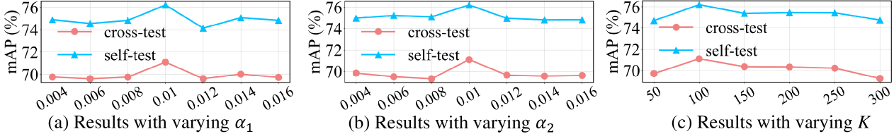
Figure 4: Experimental results of our proposed NDPP with varying scale factor ($\alpha_{1}$ and $\alpha_{2}$) and varying neighbor number ($K$) on the RParis dataset.

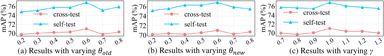
Figure 5: Experimental results of our proposed ODPP with varying threshold ($\theta_{old}$ and $\theta_{new}$) and varying loss weight ($\gamma$) on the RParis dataset.

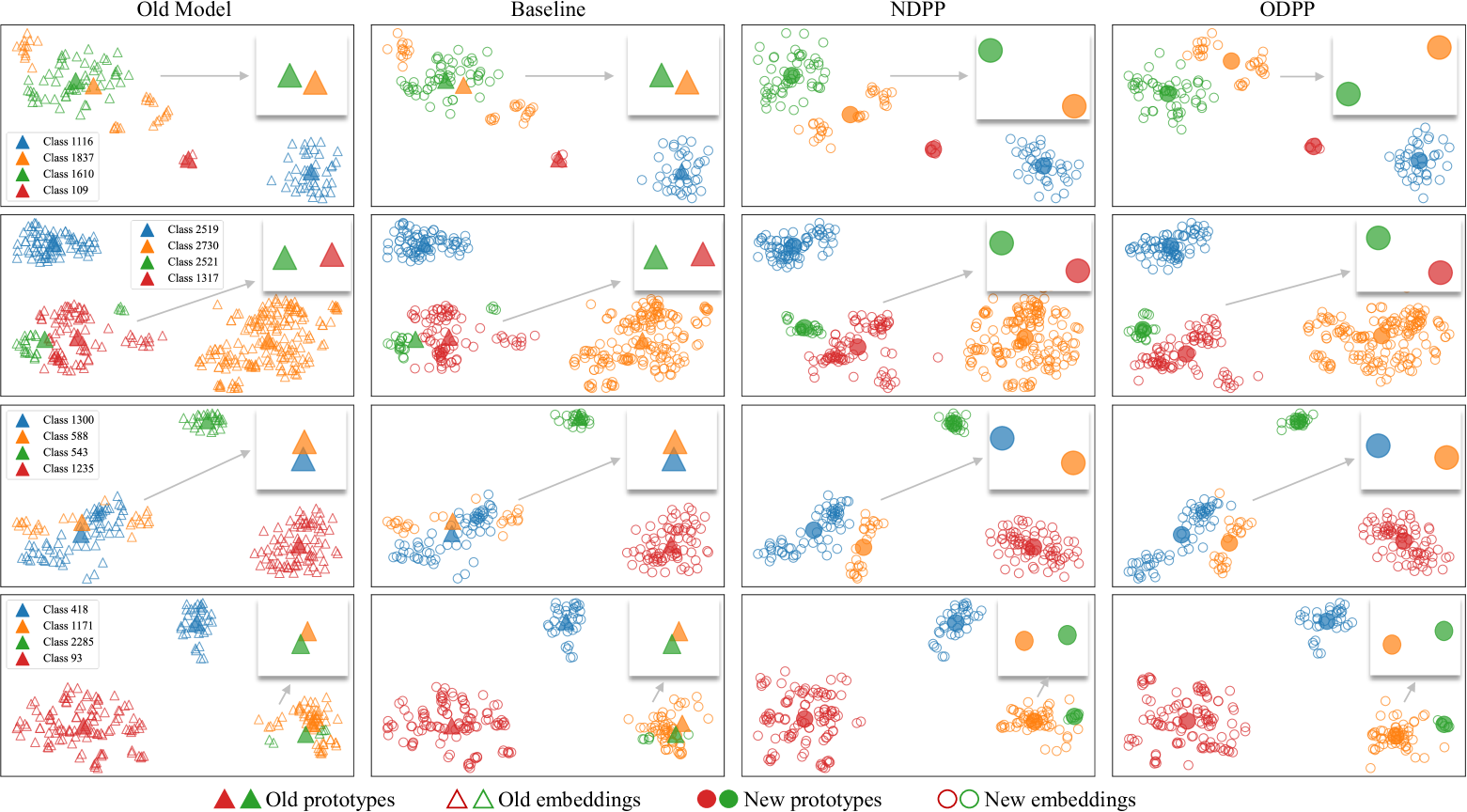
Figure 6: Distribution of the embeddings and prototypes. Compared to the Baseline, NDPP and ODPP generate more distinct embeddings. For instance, in the first row, NDPP and ODPP produce embeddings that are more distinctly separated for classes 1837 and 161 than those produced by the Baseline.

IV-E Ablation studies

To analyze our prototype perturbation methods, we conduct ablation studies for single-step backward-compatible learning on GLDv2 using the data-extension setting (9%$\rightarrow$30%).

Analyses on different perturbation methods. We analyze the effect of different perturbation methods with five variants: 1) Baseline, which performs prototype-based contrastive learning without perturbation; 2) NDPP-old, perturbing the prototypes with only old neighbors; 3) NDPP, perturbing the prototypes based on joint neighbors; 4) ODPP-old, which learns the perturbation only based on old prototypes; 5) ODPP, which learns the perturbation based on joint prototypes. Table V reports the results of the variants.

Compared with the baseline, both NDPP-old and ODPP-old improve the self-test and cross-test mAP; it demonstrates that our prototype perturbation mechanism can not only enhance the discriminative ability of the new model but also improve its backward-compatibility. Compared with NDPP-old and ODPP-old, NDPP and ODPP further improve the self-test mAP and cross-test mAP, respectively. The performance gaps manifest that the leverage of the new feature distribution benefits acquiring more effective perturbations.

Studies on hyperparameters. We also conduct studies on the hyperparameters through greedy search instead of grid search. For NDPP, we analyze the influence of the scale factors $\alpha_{1}$ and $\alpha_{2}$ as well as the neighbor number $K$. Figure 4 presents the performance of NDPP with varying hyperparameters. The model performance initially increases as the two scale factors increase and reaches the peak at both 0.01. Further increasing the scale value may introduce excessive perturbations, degenerating the performance. Besides, NDPP achieves the best result at $K=100$. For ODPP, we analyze the influence of the thresholds $\theta_{old}$ and $\theta_{new}$ as well as the balance weight $\gamma$. Figure 5 illustrates the performance of ODPP with varying hyperparameters. We can observe that the performance improves along with increasing the two thresholds and saturates at about 0.6. It implies that imposing perturbation to the prototypes less similar to others (using a lower threshold) damages the retrieval performance. In addition, ODPP obtains the best result at $\gamma\!=\!1.0$. The experimental results suggest that the importance of the old and new feature spaces in obtaining appropriate perturbations is likely to be nearly identical. Please note that our study on hyperparameters is not to obtain the best performance through hyperparameter fine-tuning. Instead, it is to demonstrate the feasibility of finding a suitable configuration to generate appropriate perturbations that can enhance the discriminative ability of the new model without compromising its compatibility.

IV-F Qualitative results

To obtain more insights into the pros and cons of our methods, we visualize the distribution of the embeddings and prototypes with t-SNE in Figure 6. The new embeddings extracted by the Baseline (w/o perturbations) cluster around the nearly indistinguishable old prototypes (e.g., classes 1837 & 1610 in the first row). As a result, it becomes difficult to differentiate the new embeddings belonging to these classes. The discriminative ability of the new model is degenerated due to the strict backward-compatible constraints. By contrast, the new embeddings extracted by NDPP and ODPP of these classes are distributed more separately, which demonstrates the effectiveness of our prototype perturbation mechanism.

V Conclusion

In this paper, we present a prototype perturbation mechanism for BCL. It allows us to align the new feature space with a pseudo-old feature space defined by the perturbed prototypes, thereby preserving the discriminative ability of the new model during BCL. Specifically, we have developed two approaches, neighbor-driven prototype perturbation and optimization-driven prototype perturbation, to implement this mechanism. We have conducted extensive experiments on the landmark and commodity datasets. Compared with state-of-the-art algorithms, our two approaches can achieve superior performance on both self-test and cross-test in most cases, demonstrating their effectiveness. Although achieving promising improvement, NDPP and ODPP leverage several hyperparameters to control the perturbations imposed on the prototype, which primarily reflects a heuristic design approach. In future work, we aim to develop backward-compatible learning methods with enhanced adaptability to the existing feature space. In future work, we aim to explore prototype perturbation or augmentation methods with superior adaptability, reducing the reliance on hyperparameters used for controlling the perturbations.

References

- [1] C. Xu, W. Wang, S. Liu, Y. Wang, Y. Tang, T. Bian, Y. Yan, Q. She, and C. Yang, “3rd place solution to google landmark recognition competition 2021,” arXiv preprint arXiv:2110.02794, pp. 1–4, 2021.
- [2] Z. Yuqi, X. Xianzhe, C. Weihua, W. Yaohua, Z. Fangyi, W. Fan, and L. Hao, “2nd place solution to google landmark retrieval 2021,” arXiv preprint arXiv:2110.04294, pp. 1–4, 2021.
- [3] M. Hendriksen, M. Bleeker, S. Vakulenko, N. van Noord, E. Kuiper, and M. de Rijke, “Extending clip for category-to-image retrieval in e-commerce,” in European Conference on Information Retrieval, 2022, pp. 289–303.
- [4] X. Jiang, Y. Yao, X. Dai, F. Shen, L. Nie, and H.-T. Shen, “Anti-collapse loss for deep metric learning,” IEEE Transactions on Multimedia, vol. 26, pp. 11 139–11 150, 2024.
- [5] T. Pan, F. Xu, X. Yang, S. He, C. Jiang, Q. Guo, F. Qian, X. Zhang, Y. Cheng, L. Yang et al., “Boundary-aware backward-compatible representation via adversarial learning in image retrieval,” in Proceedings of the IEEE/CVF Conference on Computer Vision and Pattern Recognition, 2023, pp. 15 201–15 210.
- [6] T. Weyand, A. Araujo, B. Cao, and J. Sim, “Google landmarks dataset v2-a large-scale benchmark for instance-level recognition and retrieval,” in Proceedings of the IEEE/CVF Conference on Computer Vision and Pattern Recognition, 2020, pp. 2575–2584.
- [7] L. Van der Maaten and G. Hinton, “Visualizing data using t-sne.” Journal of machine learning research, vol. 9, no. 11, 2008.
- [8] Y. Shen, Y. Xiong, W. Xia, and S. Soatto, “Towards backward-compatible representation learning,” in Proceedings of the IEEE/CVF Conference on Computer Vision and Pattern Recognition, 2020, pp. 6368–6377.
- [9] Q. Meng, C. Zhang, X. Xu, and F. Zhou, “Learning compatible embeddings,” in Proceedings of the IEEE/CVF International Conference on Computer Vision, 2021, pp. 9939–9948.
- [10] B. Zhang, Y. Ge, Y. Shen, S. Su, F. Wu, C. Yuan, X. Xu, Y. Wang, and Y. Shan, “Towards universal backward-compatible representation learning,” in Proceedings of the Thirty-First International Joint Conference on Artificial Intelligence, 7 2022, pp. 1615–1621.
- [11] J. Deng, J. Guo, N. Xue, and S. Zafeiriou, “Arcface: Additive angular margin loss for deep face recognition,” in Proceedings of the IEEE/CVF Conference on Computer Vision and Pattern Recognition, 2019, pp. 4690–4699.
- [12] F. Radenović, A. Iscen, G. Tolias, Y. Avrithis, and O. Chum, “Revisiting oxford and paris: Large-scale image retrieval benchmarking,” in Proceedings of the IEEE Conference on Computer Vision and Pattern Recognition, 2018, pp. 5706–5715.
- [13] Z. Liu, P. Luo, S. Qiu, X. Wang, and X. Tang, “Deepfashion: Powering robust clothes recognition and retrieval with rich annotations,” in Proceedings of the IEEE Conference on Computer Vision and Pattern Recognition, 2016, pp. 1096–1104.
- [14] Y. Bai, J. Jiao, Y. Lou, S. Wu, J. Liu, X. Feng, and L.-Y. Duan, “Dual-tuning: Joint prototype transfer and structure regularization for compatible feature learning,” IEEE Transactions on Multimedia, pp. 7287–7298, 2022.
- [15] B. Zhang, Y. Ge, Y. Shen, Y. Li, C. Yuan, X. Xu, Y. Wang, and Y. Shan, “Hot-refresh model upgrades with regression-free compatible training in image retrieval,” in International Conference on Learning Representations, 2021, pp. 1–20.
- [16] Y. Zhou, Z. Li, A. Shrivastava, H. Zhao, A. Torralba, T. Tian, and S.-N. Lim, “Btˆ 2: Backward-compatible training with basis transformation,” in Proceedings of the IEEE/CVF International Conference on Computer Vision, 2023, pp. 11 229–11 238.
- [17] S. Wu, L. Chen, Y. Lou, Y. Bai, T. Bai, M. Deng, and L.-Y. Duan, “Neighborhood consensus contrastive learning for backward-compatible representation,” in Proceedings of the AAAI Conference on Artificial Intelligence, vol. 36, no. 3, 2022, pp. 2722–2730.
- [18] Y. Liang, S. Zhang, Y. Wang, S. Xiao, K. Li, and X. Wang, “Mixbct: Towards self-adapting backward-compatible training,” arXiv preprint arXiv:2308.06948, pp. 1–10, 2023.
- [19] Y. K. Jang and S.-n. Lim, “Towards cross-modal backward-compatible representation learning for vision-language models,” arXiv preprint arXiv:2405.14715, pp. 1–11, 2024.
- [20] A. v. d. Oord, Y. Li, and O. Vinyals, “Representation learning with contrastive predictive coding,” arXiv preprint arXiv:1807.03748, pp. 1–13, 2018.
- [21] S. Seo, M. G. Uzunbas, B. Han, S. Cao, J. Zhang, T. Tian, and S.-N. Lim, “Online backfilling with no regret for large-scale image retrieval,” arXiv preprint arXiv:2301.03767, pp. 1–10, 2023.
- [22] H. Wu, M. Wang, W. Zhou, and H. Li, “Structure similarity preservation learning for asymmetric image retrieval,” IEEE Transactions on Multimedia, vol. 26, pp. 4693–4705, 2024.
- [23] X. Pan, H. Luo, W. Chen, F. Wang, H. Li, W. Jiang, J. Zhang, J. Gu, and P. Li, “Dynamic gradient reactivation for backward compatible person re-identification,” Pattern Recognition, vol. 146, p. 110000, 2024.
- [24] V. Ramanujan, P. K. A. Vasu, A. Farhadi, O. Tuzel, and H. Pouransari, “Forward compatible training for large-scale embedding retrieval systems,” in Proceedings of the IEEE/CVF Conference on Computer Vision and Pattern Recognition, 2022, pp. 19 386–19 395.
- [25] S. Su, B. Zhang, Y. Ge, X. Xu, Y. Wang, C. Yuan, and Y. Shan, “Privacy-preserving model upgrades with bidirectional compatible training in image retrieval,” arXiv preprint arXiv:2204.13919, pp. 1–14, 2022.
- [26] B. Zhang, S. Su, Y. Ge, X. Xu, Y. Wang, C. Yuan, M. Z. Shou, and Y. Shan, “Darwinian model upgrades: Model evolving with selective compatibility,” in Proceedings of the AAAI Conference on Artificial Intelligence, 2023, pp. 3393–3400.
- [27] F. Jaeckle, F. Faghri, A. Farhadi, O. Tuzel, and H. Pouransari, “Fastfill: Efficient compatible model update,” arXiv preprint arXiv:2303.04766, pp. 1–24, 2023.
- [28] G. I. Parisi, R. Kemker, J. L. Part, C. Kanan, and S. Wermter, “Continual lifelong learning with neural networks: A review,” Neural networks, pp. 54–71, 2019.
- [29] A. Chaudhry, M. Ranzato, M. Rohrbach, and M. Elhoseiny, “Efficient lifelong learning with a-gem,” arXiv preprint arXiv:1812.00420, pp. 1–20, 2018.
- [30] M. De Lange, R. Aljundi, M. Masana, S. Parisot, X. Jia, A. Leonardis, G. Slabaugh, and T. Tuytelaars, “A continual learning survey: Defying forgetting in classification tasks,” IEEE Transactions on Pattern Analysis and Machine Intelligence, vol. 44, pp. 3366–3385, 2021.
- [31] D.-W. Zhou, H.-L. Sun, H.-J. Ye, and D.-C. Zhan, “Expandable subspace ensemble for pre-trained model-based class-incremental learning,” in Proceedings of the IEEE/CVF Conference on Computer Vision and Pattern Recognition, June 2024, pp. 23 554–23 564.
- [32] F. Zhu, X.-Y. Zhang, C. Wang, F. Yin, and C.-L. Liu, “Prototype augmentation and self-supervision for incremental learning,” in Proceedings of the IEEE/CVF Conference on Computer Vision and Pattern Recognition, 2021, pp. 5871–5880.
- [33] T. Kim, J. Park, and B. Han, “Cross-class feature augmentation for class incremental learning,” in Proceedings of the AAAI Conference on Artificial Intelligence, vol. 38, no. 12, 2024, pp. 13 168–13 176.
- [34] M. Oh and J.-Y. Sim, “Lifelong person re-identification with backward-compatibility,” arXiv preprint arXiv:2403.10022, pp. 1–17, 2024.
- [35] Z. Cui, J. Zhou, X. Wang, M. Zhu, and Y. Peng, “Learning continual compatible representation for re-indexing free lifelong person re-identification,” in Proceedings of the IEEE/CVF Conference on Computer Vision and Pattern Recognition, 2024, pp. 16 614–16 623.
- [36] K. He, H. Fan, Y. Wu, S. Xie, and R. Girshick, “Momentum contrast for unsupervised visual representation learning,” in Proceedings of the IEEE/CVF Conference on Computer Vision and Pattern Recognition, 2020, pp. 9729–9738.
- [37] T. Chen, S. Kornblith, M. Norouzi, and G. Hinton, “A simple framework for contrastive learning of visual representations,” in International conference on machine learning. PMLR, 2020, pp. 1597–1607.
- [38] T. Chen, S. Kornblith, K. Swersky, M. Norouzi, and G. E. Hinton, “Big self-supervised models are strong semi-supervised learners,” Advances in Neural Information Processing Systems, pp. 22 243–22 255, 2020.
- [39] M. Caron, I. Misra, J. Mairal, P. Goyal, P. Bojanowski, and A. Joulin, “Unsupervised learning of visual features by contrasting cluster assignments,” Advances in Neural Information Processing Systems, pp. 9912–9924, 2020.
- [40] J.-B. Grill, F. Strub, F. Altché, C. Tallec, P. Richemond, E. Buchatskaya, C. Doersch, B. Avila Pires, Z. Guo, M. Gheshlaghi Azar et al., “Bootstrap your own latent-a new approach to self-supervised learning,” Advances in Neural Information Processing Systems, pp. 21 271–21 284, 2020.
- [41] X. Chen and K. He, “Exploring simple siamese representation learning,” in Proceedings of the IEEE/CVF Conference on Computer Vision and Pattern Recognition, 2021, pp. 15 750–15 758.
- [42] Z. Lu, L. Jin, Z. Li, and J. Tang, “Self-paced relational contrastive hashing for large-scale image retrieval,” IEEE Transactions on Multimedia, vol. 26, pp. 3392–3404, 2024.
- [43] J. Rao, L. Ding, S. Qi, M. Fang, Y. Liu, L. Shen, and D. Tao, “Dynamic contrastive distillation for image-text retrieval,” IEEE Transactions on Multimedia, vol. 25, pp. 8383–8395, 2023.
- [44] F. Shu, B. Chen, Y. Liao, J. Wang, and S. Liu, “Mac: Masked contrastive pre-training for efficient video-text retrieval,” IEEE Transactions on Multimedia, vol. 26, pp. 9962–9972, 2024.
- [45] K. He, X. Zhang, S. Ren, and J. Sun, “Deep residual learning for image recognition,” in Proceedings of the IEEE Conference on Computer Vision and Pattern Recognition, June 2016, pp. 770–778.