Scaling of Particle Heating in Shocks and Magnetic Reconnection

Abstract

Particles are heated efficiently through energy conversion processes such as shocks and magnetic reconnection in collisionless plasma environments. While empirical scaling laws for the temperature increase have been obtained, the precise mechanism of energy partition between ions and electrons remains unclear. Here we show, based on coupled theoretical and observational scaling analyses, that the temperature increase, $\Delta T$, depends linearly on three factors: the available magnetic energy per particle, the Alfvén Mach number (or reconnection rate), and the characteristic spatial scale $L$. Based on statistical datasets obtained from Earth’s plasma environment, we find that $L$ is on the order of (1) the ion gyro-radius for ion heating at shocks, (2) the ion inertial length for ion heating in magnetic reconnection, and (3) the hybrid inertial length for electron heating in both shocks and magnetic reconnection. With these scales, we derive the ion-to-electron ratios of temperature increase as $\Delta T_{\rm i}/\Delta T_{\rm e}=(3\beta_{\rm i}/2)^{1/2}(m_{\rm i}/m_{\rm e})^{1/4}$ for shocks and $\Delta T_{\rm i}/\Delta T_{\rm e}=(m_{\rm i}/m_{\rm e})^{1/4}$ for magnetic reconnection, where $\beta_{\rm i}$ is the ion plasma beta, and $m_{\rm i}$ and $m_{\rm e}$ are the ion and electron particle masses, respectively. We anticipate that this study will serve as a starting point for a better understanding of particle heating in space plasmas, enabling more sophisticated modeling of its scaling and universality.

1 Introduction

Table 1: Empirically derived scaling of particle heating during reconnection.

Species	Relation	Region	Plasma beta	Alfvén speed $V_{\rm A}$	Mission	Reference
ions	ΔT_i ∼0.13    m_iV_A^2	magnetopause	β_i ∼0.2 - 550	$<600$ km/s	THEMIS	PhanTD_2014_Ion
ions	ΔT_i ≲0.13    m_iV_A^2	magnetotail	β_i ∼0.003 - 1	$800-4000$ km/s	MMS	OierosetM_2024_Scaling
electrons	ΔT_e ∼0.017  m_iV_A^2	magnetopause	β_e ∼0.1 - 10	$<600$ km/s	THEMIS	PhanTD_2013_Electron
electrons	ΔT_e ∼0.020  m_iV_A^2	magnetotail	β_e ∼0.001 - 0.1	$800-4000$ km/s	MMS	OierosetM_2023_Scaling

Note. — The data were obtained by NASA’s spacecraft missions, Time History of Events and Macroscale Interactions during Substorms (THEMIS) (AngelopoulosV_2008_THEMIS) and Magnetospheric MultiScale (MMS) (BurchJL_2016_Magnetospheric).

Particles – both ions and electrons – are heated efficiently through fundamental plasma processes such as shocks and magnetic reconnection in space, solar, and astrophysical plasma environments (e.g. TidmanDA_1971_Shock; TsurutaniBT_1985_Collisionless; LinY_1994_Structure; KivelsonMG_1995_Introduction; PriestE_2000_Magnetic; AschwandenMJ_2005_Physics; ZweibelEG_2009_Magnetic; LongairMS_2011_High; EastwoodJP_2013_Energy). A challenge is that, at magnetohydro-dynamic (MHD) scales, the conservation laws can only predict the total temperature on the downstream side. It remains unclear how the upstream energy is partitioned between ions and electrons during the energy conversion processes such as shocks and magnetic reconnection, despite extensive studies with observations and simulations as summarized below.

For non-relativistic collisionless shocks, the Rankine-Hugoniot (RH) relations reveal that, for the strong shock limit with the shock compression ratio of 4, the increase of the total temperature is approximated as $\Delta T\sim(3/16)m_{\rm i}V_{\rm in}^{2}$, where $m_{\rm i}$ is the proton mass and $V_{\rm in}$ is the bulk flow speed of the upstream, incoming plasma in the shock-rest, shock normal incidence frame (e.g. TidmanDA_1971_Shock; GhavamianP_2013_ElectronIon). Because of the large ion-to-electron mass ratio, this total temperature change is comparable to the ion temperature change, $\Delta T\sim\Delta T_{\rm i}$. For electron heating, previous studies have identified that the increase of the electron temperature $\Delta T_{\rm e}$ correlates with the change of bulk flow energy, as well as the shock potential (e.g. ThomsenMF_1987_Strong; SchwartzSJ_1988_Electron; HullAJ_2000_Electron). For example, it was reported that $\Delta T_{\rm e}\sim 0.057\,\Delta\left(m_{\rm i}V_{n}^{2}/2\right)$, where $V_{n}$ is the bulk flow velocity along the shock normal direction $\mathbf{\hat{n}}$ and $\Delta(m_{\rm i}V_{n}^{2}/2)$ is the change of bulk flow energy across the shock front (HullAJ_2000_Electron). Interestingly, a compilation of statistical data from Earth’s and Saturn’s bow shock shows that the temperature ratio $T_{\rm e}/T_{\rm i}$ on the downstream side decreases from $\sim$1 to $\sim$0.1 as the Alfvén or magnetosonic Mach number on the upstream side increases from $\sim$1 to $\sim$10 (GhavamianP_2013_ElectronIon). To interpret this observational relation, a thermodynamic relation for the minimum values of $T_{\rm e}/T_{\rm i}$ have been derived (VinkJ_2015_electronion), and various particle simulations have been conducted (e.g. TranA_2020_Electron; BohdanA_2020_Kinetic). A possible extension to astrophysical parameter ranges is also important (e.g. GhavamianP_2013_ElectronIon; RaymondJC_2023_Electron).

For magnetic reconnection, in-situ observations in Earth’s magnetosphere have shown that $\Delta T$ depends roughly linearly on available magnetic energy per particle $m_{\rm i}V_{\rm A}^{2}$, as summarized in Table 1, where $V_{\rm A}$ is the Alfvén speed measured in the upstream inflow region with inflow density and inflow magnetic field strength (PhanTD_2013_Electron; PhanTD_2014_Ion; OierosetM_2023_Scaling; OierosetM_2024_Scaling). It is evident that the scaling applies over large ranges of plasma $\beta$ and $V_{\rm A}$. Theories indicate that a similar linear dependence $\Delta T_{\rm i}=(1/3)m_{\rm i}V_{\rm A}^{2}$ arises from Alfvénic counter-streaming proton beams in the exhaust (DrakeJF_2009_Ion) and that the difference from the observations in the factor for the scaling can be attributed to the fact that the observed outflow jets are not always being fully Alfvénic (HaggertyCC_2015_competition; HaggertyCC_2018_reduction) due to the presence of electric potentials in the reconnection exhaust (e.g. EgedalJ_2005_situ; EgedalJ_2013_review). For electron heating, a linear dependence of $\Delta T_{\rm e}\sim 0.03-0.05m_{\rm i}V_{\rm A}^{2}$ has been obtained by particle simulations (ShayMA_2014_Electron; HaggertyCC_2015_competition).

In this Paper, we propose an alternative approach to interpreting and predicting particle heating at shocks and in reconnecting current sheets. We propose that heating is a function of the available magnetic energy per particle, the Alfvén Mach number, and the characteristic spatial scale. Heating is defined as an increase in temperature, which corresponds to the second-order moment of the velocity distribution in the plasma rest frame. The paper is organized as follows. In Section 2, we deduce and normalize the expression. Then, the validity of the idea is tested against observations of quasi-perpendicular shocks (Section 3) and magnetic reconnection (Section 4). Finally, we summarize and discuss the results in Section 5.

2 Theoretical expression for particle heating

In general, an energization $\Delta\varepsilon$ of a charged particle can be expressed as $\Delta\varepsilon=qVBL$ where $q$ is the particle charge, $VB$ is the motional electric field constructed from the characteristic flow speed $V$ and magnetic field $B$, and $L$ is the distance of travel during energization. This is a ballpark estimate with an assumption the bulk flow $\mathbf{V}$ and the magnetic field $\mathbf{B}$ are perpendicular to each other. A similar expression has been used in the context of particle acceleration to non-thermal energies (e.g. HillasM_1984_Origin; MatthaeusWH_1984_Particle; OkaM_2025_Maximum) and the rate of explosive energy release in Earth’s magnetotail (OkaM_2022_Electron).

To better illustrate the physical processes involved in energization, we further rewrite this expression by normalizing $V$ and $L$ by $V_{\rm A}$ and the ion inertial length $d_{\rm i}$, respectively. We also convert kinetic energy $\varepsilon$ to temperature $T$ via $T=(2/f)\varepsilon$ where $f$ is the degrees of freedom and is chosen to be $f=3$ throughout this paper. Then, we obtain

$$\Delta T=\frac{2}{f}\left(\frac{V}{V_{\rm A}}\right)\left(\frac{L}{d_{\rm i}}\right)m_{\rm i}V_{\rm A}^{2}$$ (1)

Therefore, any scaling for heating should be explained by three physical parameters: (1) the degrees of freedom $f$, (2) the normalized flow speed $V/V_{\rm A}$, typically referred to as the Alfvén Mach number $M_{\rm A}$ or reconnection rate $\alpha_{\rm R}$, and (3) the characteristic spatial scale $L/d_{\rm i}$. The quantity $m_{\rm i}V_{\rm A}^{2}$ is an environmental parameter that depends on the density $N$ and magnetic field strength $B$. It is derived by dividing the incoming Poynting flux by the inflowing particle density flux (e.g. ShayMA_2014_Electron) and therefore represents the magnetic energy per particle that is available in the upstream region of a shock or a reconnecting current sheet. It can also be used to normalize the temperature $\Delta T$.

All these parameters, except $L$, are based on upstream values and are also observable, although there may be some uncertainty in the measurement of the reconnection rate $\alpha_{\rm R}$. The parameter $L$ is not directly known, but various characteristic lengths, such as the gyro-radius and inertial length, can be considered to calculate the predicted heating from Eq.(2) and compare with observational data to deduce the most appropriate scale for $L$. As we shall see in the following section, the values of $L$ are typically on the order of the ion kinetic scale for ion heating and the hybrid inertial length for electron heating. It is also worth noting that $L/d_{\rm i}$ can be replaced with $\Omega_{\rm ci}\tau_{\rm A}$, where $\Omega_{\rm ci}$ is the ion cyclotron frequency and $\tau_{\rm A}$ is the Alfvén transit time. This alternative formulation is useful when interpreting the time evolution of particle energization (e.g. MatthaeusWH_1984_Particle).

3 Application of the formula to shocks

We first apply Eq.(1) to the physics of non-relativistic collisionless shocks. Using $f=3$ and $M_{\rm A}=V_{\rm in}/V_{\rm A}$, where $V_{\rm in}$ is the incoming flow speed in the shock normal incidence frame, one obtains

$$\Delta T=\frac{2}{3}M_{\rm A}\left(\frac{L}{d_{\rm i}}\right)m_{\rm i}V_{\rm A}^{2}$$ (2)

As noted in the previous section, all quantities except $L$ are observable. Therefore, we use observational datasets to find reasonable values for $L$. Specifically, we analyzed 80 cases of supercritical, quasi-perpendicular bow shock crossings obtained by the Magnetospheric MultiScale (MMS) mission.

These events were selected through visual inspection, with upstream and downstream time periods defined to calculate the temperature increases for both ions ($\Delta T_{\rm i}$) and electrons ($\Delta T_{\rm e}$). We focused on super-critical shocks because they are much more frequently observed. Also, we avoided the events that are confounded by upstream-escaping particles, resulting in a bias toward quasi-perpendicular shocks.

While more details of our event selection and analysis procedures are described in Appendix, we present here an example crossing event, shown in Figure 1 (left), observed on 2019 October 26. In this event, MMS traversed from upstream to downstream and detected a significant increase in ion and electron temperatures (Fig.1f) accompanied by similarly abrupt changes in the magnetic field (Fig.1a), density (Fig.1e), and flow velocity (Fig.1g). We then selected stable intervals, highlighted by the vertical lines, to determine upstream and downstream plasma parameters, especially the temperatures. The upstream interval was carefully chosen between the magnetic field direction change at 19:44:30 and the leading edge of the region of reflected-gyrating ions (Fig.1c). We repeated this procedure for all events and performed a statistical analysis, as described below.

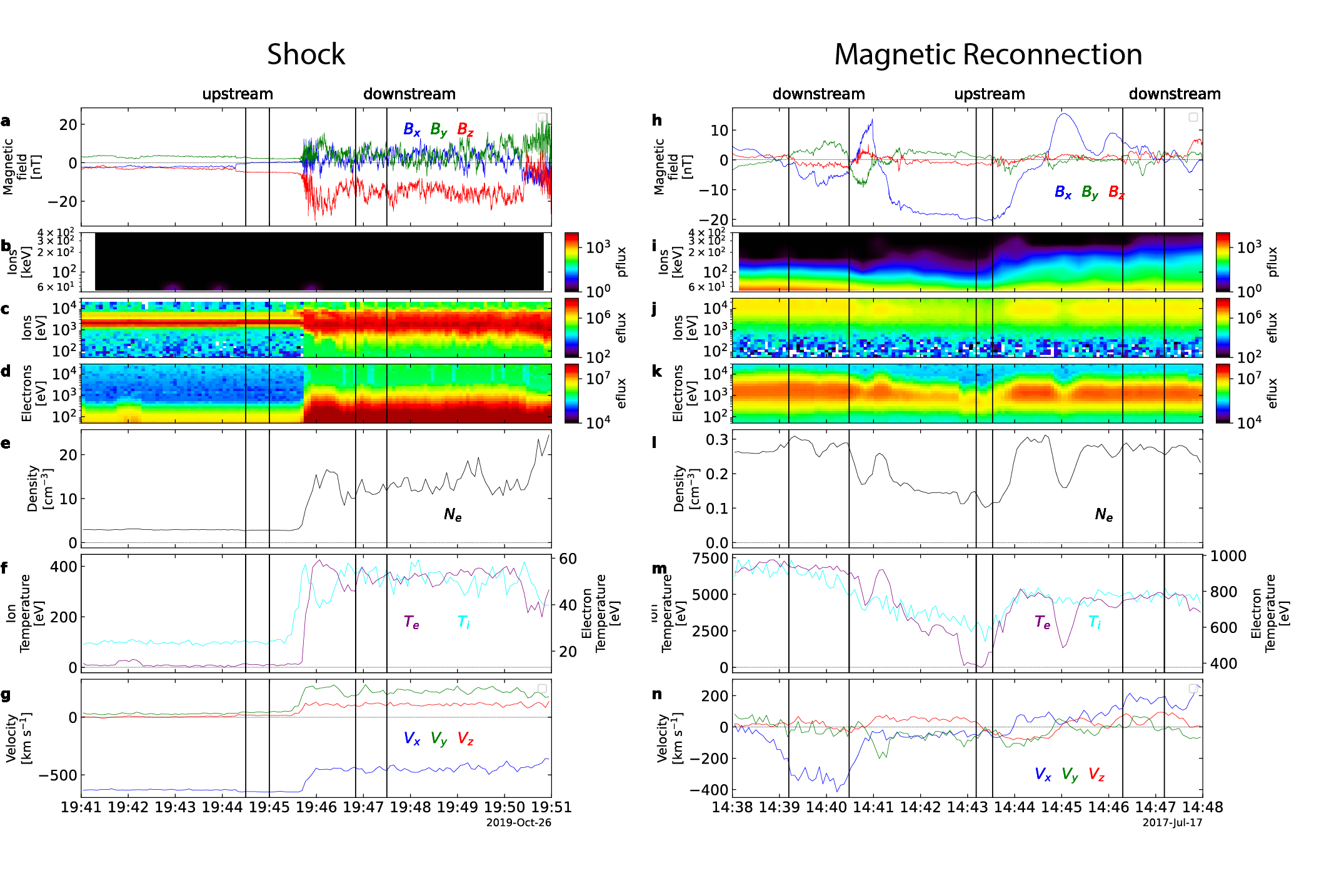
Figure 1: Plasma parameters of example shock (left) and reconnection (right) events, demonstrating our procedure of event identification and analysis. From top to bottom are (a,h) magnetic field vector, (b,i) energetic ion spectrogram, (c,j) ion spectrogram, (d,k) electron spectrogram, (e, l) electron density, (f, m) ion and electron temperatures, (g, n) ion bulk flow vector. For the color scale in spectrograms, pflux and eflux represent particle flux (cm${}^{-2}$s${}^{-1}$sr${}^{-1}$keV${}^{-1}$) and energy flux (keV cm${}^{-2}$s${}^{-1}$sr${}^{-1}$keV${}^{-1}$), respectively.

Figure 2 shows the results of our statistical analysis for both ions (upper panels) and electrons (lower panels). For ions, we first examined the validity of the classical scaling $\Delta T\sim\Delta T_{\rm i}\sim(3/16)m_{\rm i}V_{\rm in}^{2}$. To this end, we have introduced a multiplicative factor $C$ to assume $\Delta T_{\rm i}=C(3/16)m_{\rm i}V_{\rm in}^{2}$ and performed a linear regression to derive the best-fit value of $C$. For the linear regression, we used the average values and standard deviations calculated for each dataset, separated into bins. Figure 2a shows the result. It is evident that the classical scaling works with the best-fit value of $C\sim 0.88$, close to but somewhat less than the expected value of 1.

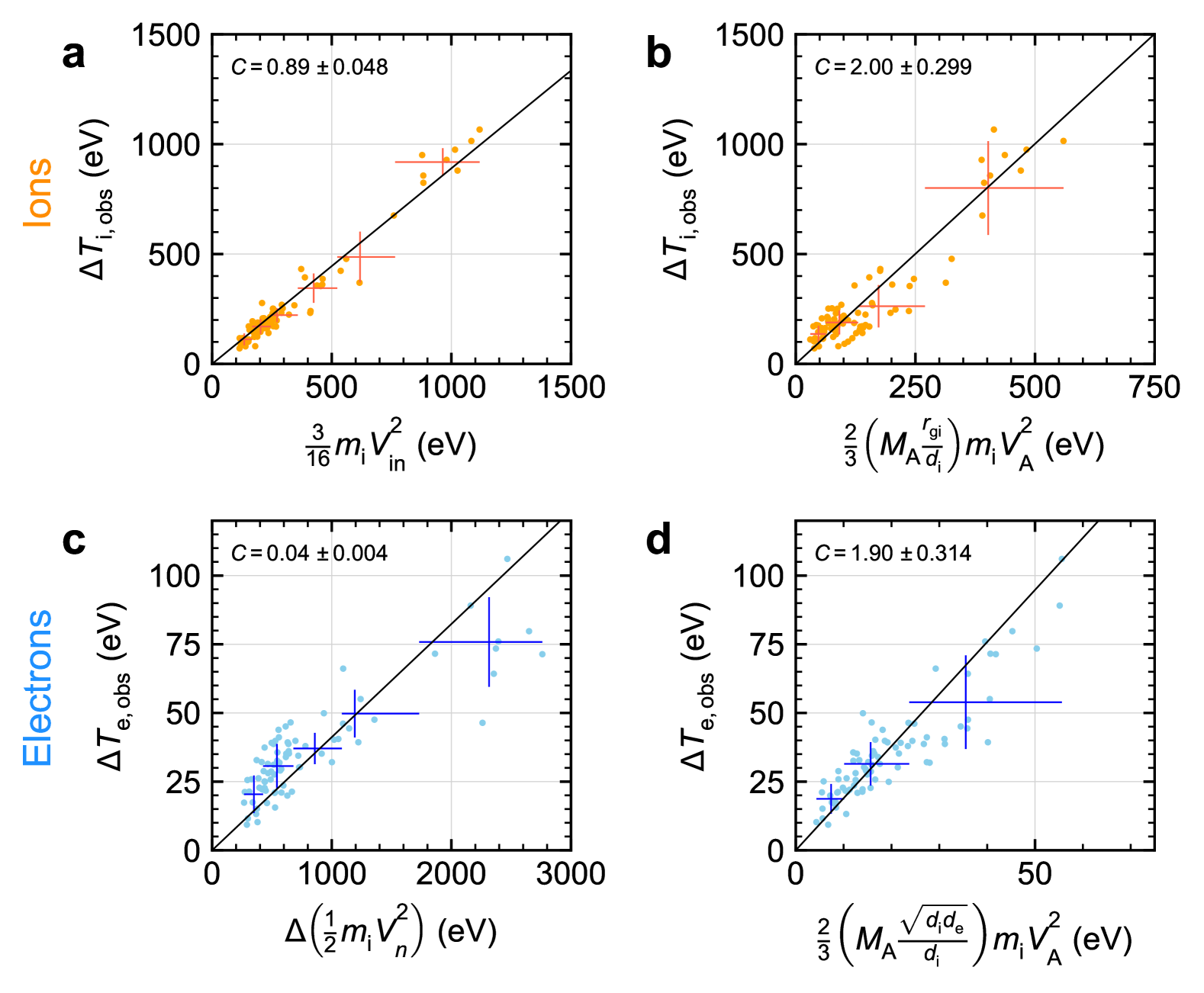
Figure 2: Scaling of the temperature increase across Earth’s bow shock for ions (upper panels) and electrons (lower panels). A new approach using Eq.(2) (right panels) is compared to an earlier approach of using the bulk flow energy (left panels). The titles of the horizontal axes indicate the formula used to predict the temperature increase. The multiplication factor $C$ is derived through linear regression and illustrated by the thin black line.

We then tested Eq.(2) more directly by comparing with observations with different choices of $L$, such as the ion inertial length $d_{\rm i}$ and the gyro-radius based on the upstream ion thermal speed $r_{\rm gi}$. More precisely, we again introduced a multiplicative factor $C$ and derived the best-fit value of $C$ for $L=Cd_{\rm i}$ and $L=Cr_{\rm gi}$. We obtained $L\sim 2.5d_{\rm i}$ with c.c. = 0.79, and $L\sim 2.00r_{\rm gi}$ with c.c.=0.93, where c.c. is the Pearson correlation coefficient. Therefore, we conclude that Eq.(2) with $L=2r_{gi}$ gives a reasonable, semi-empirically-derived formula for ion heating at shocks, and this is shown in Figure 2b. We could also try the ion gyro-radius based on the incoming flow speed $r_{\rm gi0}=V_{\rm in}/\Omega_{\rm ci}$ and the foot size $L_{\rm foot}$ as formulated by LiveseyWA_1984_comparison. However, with these parameters, Eq.(2) reduces to $\Delta T_{\rm i}\propto m_{\rm i}V_{\rm in}^{2}$, which is essentially the same as the classical scaling of $\Delta T_{\rm i}\sim(3/16)m_{\rm i}V_{\rm in}^{2}$. In fact, this classical scaling can be obtained by inserting $L=(9/32)r_{\rm gi0}\sim(1/4)r_{\rm gi0}$ into Eq.(2).

If we further introduce the ion plasma beta $\beta_{\rm i}$, the formula can be rewritten as

$$\Delta T_{\rm i}=\frac{4}{3}M_{\rm A}\left(\frac{3}{2}\beta_{\rm i}\right)^{\frac{1}{2}}m_{\rm i}V_{\rm A}^{2}$$ (3)

where we used the relation $r_{\rm gi}/d_{\rm i}=v_{\rm thi}/V_{\rm A}=(3\beta_{\rm i}/2)^{1/2}$. Here, $v_{\rm thi}$ is the upstream ion thermal speed defined as the root-mean-square speed of the three-dimensional Maxwellian velocity distribution, i.e., $v_{\rm thi}=\sqrt{3k_{B}T/m}$, where $k_{B}$ is the Boltzman constant.

For electrons (lower panels), we again started from validating earlier results. Figure 2c tests an earlier idea that $\Delta T_{\rm e}$ depends on the change of bulk flow energy $\Delta(m_{\rm i}V_{n}^{2}/2)$ across the shock front (e.g. SchwartzSJ_1988_Electron; HullAJ_2000_Electron). We found that $\Delta T_{\rm e}$ increases linearly with $\Delta(m_{\rm i}V_{n}^{2}/2)$ , with a slope of $C\sim 0.04$, which is comparable to but somewhat smaller than $\sim$0.06 reported by HullAJ_2000_Electron. This difference appears to be due to the fact that, in our cases, the observed values of $\Delta T_{\rm e}$ increased progressively less as $\Delta(m_{\rm i}V_{n}^{2}/2)$ increased.

For the application of Eq.(2), we tested a variety of different parameters such as electron inertial length $d_{\rm e}$, electron gyro-radius $r_{\rm ge}$, the hybrid inertial length $\sqrt{d_{\rm i}d_{\rm e}}$ and hybrid gyro-radius $\sqrt{r_{\rm gi}r_{\rm ge}}$. With the linear regression analysis, we obtained $L=(12.4\pm 2.1)d_{\rm e}$ with c.c. $=0.90$ and $L=(9.8\pm 1.6)r_{\rm e}$ with c.c.$=0.88$, indicating that the electron scale underestimates the spatial scale and hence electron heating by an order of magnitude. In contrast, the hybrid scale provides a better estimate as we obtained $L=(1.90\pm 0.31)\sqrt{d_{\rm i}d_{\rm e}}$ with c.c. $=0.90$ and $L=(1.55\pm 0.26)\sqrt{r_{\rm gi}r_{\rm ge}}$ with c.c. $=0.87$. While $\sqrt{d_{\rm i}d_{\rm e}}$ and $\sqrt{r_{\rm gi}r_{\rm ge}}$ are comparable, we adopt $\sqrt{d_{\rm i}d_{\rm e}}$ because it produces a slightly higher c.c., and the formula remains simple. Then, within the error range, electron heating at shocks can be reasonably modeled by Eq.(2) with $L=2\sqrt{d_{\rm i}d_{\rm e}}$. Figure 2d shows the regression analysis for the choice of $\sqrt{d_{\rm i}d_{\rm e}}$. Because of the relation $\sqrt{d_{\rm i}d_{\rm e}}/d_{\rm i}=\sqrt{d_{\rm e}/d_{\rm i}}=(m_{\rm i}/m_{\rm e})^{-1/4}$, the formula can be expressed as

$$\Delta T_{\rm e}=\frac{4}{3}M_{\rm A}\left(\frac{m_{\rm i}}{m_{\rm e}}\right)^{-\frac{1}{4}}m_{\rm i}V_{\rm A}^{2}$$ (4)

By using the derived formula for ions and electrons, we can examine the electron-to-ion ratio of downstream temperature ($T_{\rm e}/T_{\rm i}$) using both observations and predictions based on Eq.(2), as shown in the upper panels of Figure 3. Figure 3a is obtained from our observational MMS dataset and is consistent with GhavamianP_2013_ElectronIon who reported that $T_{\rm e}/T_{\rm i}$ on the downstream side decreases from $\sim$1 to $\sim$0.1 as the upstream Alfvén Mach number increases from $\sim$1 to $\sim$10. Figure 3b shows the prediction based on our formulas with $L=2r_{\rm gi}$ for ions and $L=2\sqrt{d_{\rm i}d_{\rm e}}$ for electrons. When compared to the observation (Figure 3a), it is evident that our simple formula reproduces the empirical scaling well and that $T_{\rm e}/T_{\rm i}$ correlates with $M_{\rm A}$.

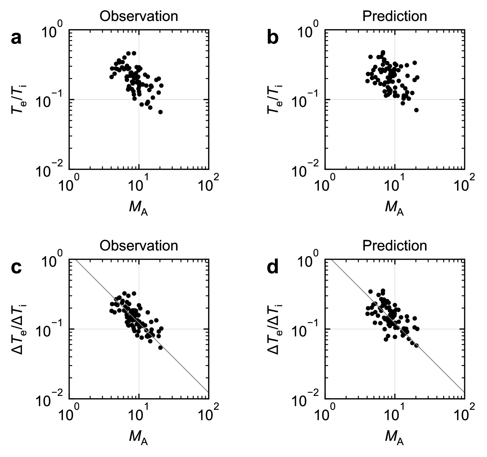
Figure 3: The $M_{\rm A}$ dependence of the electron-to-ion ratios of temperatures (upper panels) and temperature increases (lower panels), obtained from observations at Earth’s bow shock (left panels) and predictions based on Eq.(2) (right panels). While each observational data point (filled circle) corresponds to a different value of $\psi$, the relation expressed by Eq.(7) for $\psi=8$ is shown by the thin gray curve.

Figures 3(c,d) show the $M_{\rm A}$ dependencies for $\Delta T_{\rm e}/\Delta T_{\rm i}$ instead of $T_{\rm e}/T_{\rm i}$. Again, a similar linear relation was obtained for both observations (Figure 3c) and predictions (Figure 3d). The origin of this $M_{\rm A}$-dependence can be understood when we combine the formulas, i.e., Eq.(2) with $L=2r_{\rm gi}$ for $\Delta T_{\rm i}$ and $L=2\sqrt{d_{\rm i}d_{\rm e}}$ for $\Delta T_{\rm e}$, to obtain

$$\frac{\Delta T_{\rm e}}{\Delta T_{\rm i}} =\frac{\sqrt{d_{\rm i}d_{\rm e}}}{r_{\rm gi}}$$ (5)

$$=\frac{V_{\rm A}}{v_{\rm thi}}\left(\frac{m_{\rm i}}{m_{\rm e}}\right)^{-\frac{1}{4}}$$ (6)

$$=\psi\left(\frac{m_{\rm i}}{m_{\rm e}}\right)^{-\frac{1}{4}}M_{\rm A}^{-1}$$ (7)

where we introduced $\psi=V_{\rm in}/V_{\rm thi}$. Therefore, the empirically known linear relationship between $T_{\rm e}/T_{\rm i}$ (or equivalently $\Delta T_{\rm e}/\Delta T_{\rm i}$) and $M_{\rm A}$ is attributed to the characteristic of the solar wind, in which $\psi$ vary less than $M_{\rm A}$. In our dataset, $\psi$ ranges from $\sim$3 to $\sim$20, with a typical value of $\sim$8. The gray lines in Figure 3(c,d) show the prediction from Eq.(7) with a fixed value of $\psi=8$. The predicted data points (filled circles) in Figure 3 are based on observed values of $\psi$, which vary from $\sim 3$ to $\sim 20$.

Furthermore, the above expressions, in particular Eq.(6), or a direct comparison between Eqs. (3) and (4) reveal that the previously-known $M_{A}$ dependence is intrinsically a $\beta_{\rm i}$ dependence. In fact, $\beta_{\rm i}=(2/3)(v_{\rm thi}/V_{\rm A})^{2}=(2/3)\psi^{-2}M_{\rm A}^{2}$ and this relation in the upstream parameters can be confirmed with our dataset (Appendix). Consequently, we arrive at

$$\frac{\Delta T_{\rm i}}{\Delta T_{\rm e}}=\left(\frac{3}{2}\beta_{\rm i}\right)^{\frac{1}{2}}\left(\frac{m_{\rm i}}{m_{\rm e}}\right)^{\frac{1}{4}}$$ (8)

where we deliberately considered $\Delta T_{\rm i}/\Delta T_{\rm e}$ instead of $\Delta T_{\rm e}/\Delta T_{\rm i}$ to avoid using negative indices and to more easily compare with the same ratio of temperature increase for magnetic reconnection derived in the next section.

Figure 4 shows such a $\beta_{i}$ dependence of $\Delta T_{\rm i}/\Delta T_{\rm e}$ obtained from both observations (filled circles) and the above expression (gray line). It is evident that the observation matches well with the derived formula.

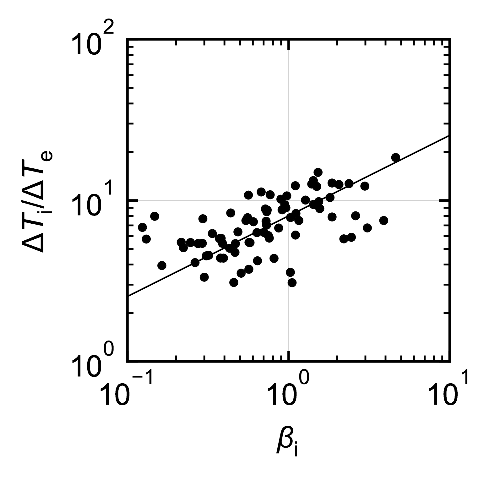
Figure 4: The $\beta_{\rm i}$ dependence of the electron-to-ion ratio of temperature increase. The observations at Earth’s bow shock are shown by the filled circles, whereas the derived formula of $\Delta T_{\rm i}/\Delta T_{\rm e}=(3\beta_{\rm i}/2)^{1/2}(m_{\rm i}/m_{\rm e})^{1/4}$ is indicated by the black line.

4 Application of the formula to magnetic reconnection

Let us now consider how the expression (1) applies to magnetic reconnection. We use the normalized reconnection rate $\alpha_{\rm R}=V_{\rm in}/V_{\rm A}$ where $V_{\rm in}$ is the reconnection inflow speed, so that Eq.(1) becomes

$$\Delta T=\frac{2}{3}\alpha_{\rm R}\left(\frac{L}{d_{\rm i}}\right)m_{\rm i}V_{\rm A}^{2}$$ (9)

Unfortunately, unlike the observations of Earth’s bow shock where $M_{\rm A}$ can be measured directly, it is challenging to measure $\alpha_{\rm R}$ in Earth’s magnetosphere because the plasma density becomes very low in the inflow region. Nevertheless, recent careful analysis with different methodologies reported $\alpha_{\rm R}$ values in a range of $0.15-0.20$ (e.g. NakamuraTKM_2018_Measurement; GenestretiKJ_2018_How). In fact, a recent theoretical study argued that $\alpha_{\rm R}$ is a function of the opening angle made by the upstream magnetic fields and that it could be as high as $\alpha_{\rm R}\sim$ 0.2 (LiuYH_2017_Why). On the other hand, many simulation studies have established the canonical value of $\alpha_{\rm R}\sim 0.1$ (e.g. ShayMA_1999_scaling; BirnJ_2001_Geospace; LiuYH_2022_Firstprinciples). Therefore, throughout this paper, we assume $\alpha_{\rm R}=0.1$ and explore different values of $L$. We shall keep in mind, however, that it is the product $\alpha_{\rm R}(L/d_{\rm i})$ that can be constrained by observations. It is very plausible that $\alpha_{\rm R}$ is $0.2$ and, in such a case, any values of $L$ we deduce in this paper should be reduced by half.

With this caveat in mind, we revisited previous statistical studies of plasma heating, summarized in Table 1. Figure 1 (right) shows an example crossing of magnetotail reconnection observed by MMS on 2017 July 17 (e.g. OkaM_2022_Electron; OierosetM_2023_Scaling; OierosetM_2024_Scaling). A flow reversal from tailward ($V_{\rm x}<0$) to earthward ($V_{\rm x}>0$) indicates that the X-line passed by the spacecraft in the plasma sheet with relatively small $B_{\rm x}$ (Fig.1n). During the X-line passage, the spacecraft entered into a region of enhanced $B$ and depressed $N$, $T$, and $V$, indicating that the spacecraft moved into the lobe region temporarily. The periods of fast flows in the plasma sheet and the excursion to the lobe are highlighted by the vertical lines and marked as downstream and upstream respectively. The plasma temperatures averaged over these intervals are used to derive the temperature increase across reconnection. Essentially the same process was repeated for 20 magnetotail reconnection events reported by OierosetM_2023_Scaling; OierosetM_2024_Scaling as well as 103 magnetopause reported by PhanTD_2013_Electron; PhanTD_2014_Ion, although the magnetopause events are some what complicated due to the asymmetry in the inflow direction. See Appendix for more details and the full lists of events.

As in Section 3, we first attempted to reproduce earlier findings. Figure 5 shows the observed values of ion heating $\Delta T_{\rm i}$ (upper panels) and electron heating $\Delta T_{\rm e}$ (lower panels) as a function of $m_{\rm i}V_{\rm A}^{2}$ in logarithmic (left panels) and linear (right panels) scales. The data points from both magnetopause and magnetotail events are combined so that they are spread over a wide range of values, as demonstrated in the logarithmic plots. The linear plots are shown because there were three negative values of $\Delta T_{\rm i}$ and six negative values of $\Delta T_{\rm e}$. The linear format also enhances the deviation of $\Delta T_{\rm i}$ from the overall trend for larger values of $m_{\rm i}V_{\rm A}^{2}$, as already reported by OierosetM_2023_Scaling. The slopes obtained through linear regression of all data points including negative values are annotated at the top left corner of each panel, and they are consistent with the reported values (Table 1) within the error ranges.

Then, if we choose $L=2d_{\rm i}$ for ion heating and insert this into Eq.(9), we immediately obtain

$$\Delta T_{i}=\frac{2}{15}\,m_{\rm i}V_{\rm A}^{2}\sim 0.13\,m_{\rm i}V_{\rm A}^{2}$$ (10)

which is identical to the ion heating scaling of $0.13\,m_{\rm i}V_{\rm A}^{2}$ obtained by PhanTD_2014_Ion, OierosetM_2024_Scaling, and our combined analysis described above. Also, if we introduce a hybrid scale of $L=2\sqrt{d_{\rm i}d_{e}}$ for electron heating, we obtain

$$\Delta T_{e}=\frac{2}{15}\left(\frac{m_{\rm i}}{m_{\rm e}}\right)^{-\frac{1}{4}}m_{\rm i}V_{\rm A}^{2}\sim 0.020\,m_{\rm i}V_{\rm A}^{2}$$ (11)

This is exactly the same as the scaling of $\sim 0.020\,m_{\rm i}V_{\rm A}^{2}$ obtained by OierosetM_2023_Scaling and our combined analysis described above, and also consistent with $\sim 0.017\,m_{\rm i}V_{\rm A}^{2}$ reported by PhanTD_2013_Electron. The value $L=2d_{e}$ would underestimate the electron heating because $d_{e}/d_{\rm i}\sim\sqrt{m_{e}/m_{\rm i}}$ and we obtain $\Delta T_{e}\sim 1.5\times 10^{-3}\,m_{\rm i}V_{\rm A}^{2}$, an order of magnitude smaller than what we expect $\sim 0.02$.

Following our analysis in Section 3, we can again introduce a multiplicative parameter $C$ and hence $L=Cd_{\rm i}$ to obtain $\Delta T_{\rm i}=C(1/15)m_{\rm i}V_{\rm A}^{2}$ for ion heating. Using the statistically-derived slope, we immediately obtain $C=1.82\pm 0.249$ with c.c.$=0.88$. Therefore, within the error range, we can reasonably justify the use of $L=2d_{\rm i}$ in the above formula.

We also note that $d_{\rm i}$ is often comparable to the ion gyro-radius $r_{\rm gi,out}$ in the plasma sheet, defined with the ion thermal speed in the outflow region. This suggests that $\Delta T_{\rm i}$ can be approximated with $L=2r_{\rm gi,out}$. Figure 6(a,b) demonstrates that this alternative prediction with $L=Cr_{\rm gi,out}$ yields a multiplicative factor of $C=1.97\pm 0.37$ with c.c.$=0.95$, supporting this expectation. Figure 6c further demonstrates that the ratio of $r_{\rm gi,out}/d_{\rm i}$ is indeed comparable to $\sim$1, especially when $m_{\rm i}V_{\rm A}^{2}$ is in the range of $0.1-10$. However, this ratio deviates significantly when $m_{\rm i}V_{\rm A}^{2}$ is either below 0.1 or above 10. Moreover, in deriving our heating formula from a predictive standpoint, it is more reasonable to use $d_{\rm i}$, an upstream parameter, rather than $r_{\rm gi,out}$, a downstream parameter. Therefore, we retain the use of $d_{\rm i}$ in our formula.

For electron heating, we assume $L=C\sqrt{d_{\rm i}d_{\rm e}}$ to obtain $\Delta T_{e}=C(1/15)(m_{\rm i}/m_{\rm e})^{-1/4}m_{\rm i}V_{\rm A}^{2}$. The best-fit value $C$ that corresponds to the derived slope is $C=1.739\pm 0.258$ with c.c.$=0.98$. The error range allows for a maximum of $C=1.998$, indicating that the derived value of $C$ is somewhat smaller than our assumed value of $C=2$ used in deriving the formula. This deviation likely originates from the magnetopause data, which suggests the relation of $\Delta T_{\rm e}\sim 0.017m_{\rm i}V_{\rm A}^{2}$ (PhanTD_2013_Electron) instead of $\Delta T_{\rm e}\sim 0.020m_{\rm i}V_{\rm A}^{2}$. In fact, using the magnetotail data alone resulted in $C=1.96\pm 0.362$. Given the complexity of analyzing magnetopause reconnection arising from asymmetry in the inflow direction, we retain our assumption of $C=2$ and defer more refined observational and theoretical studies to future work. This is a reasonable choice, especially because, as we shall see below, the temperature ratio $\Delta T_{\rm i}/\Delta T_{\rm e}$ with the assumption of $C=2$ matches with the one derived from an independent theoretical study.

To explore potential alternative assumptions, we also consider $L=C\sqrt{r_{\rm gi}r_{\rm ge}}$, which yields $C=1.50\pm 0.379$ with c.c. $=0.88$ and increases the complexity of the formula, similar to the case for shocks. While this alternative may be worth further investigation, its slightly lower agreement with the data and the increased complexity of the formula support our choice of $L=2\sqrt{d_{\rm i}d_{\rm e}}$ in the present study.

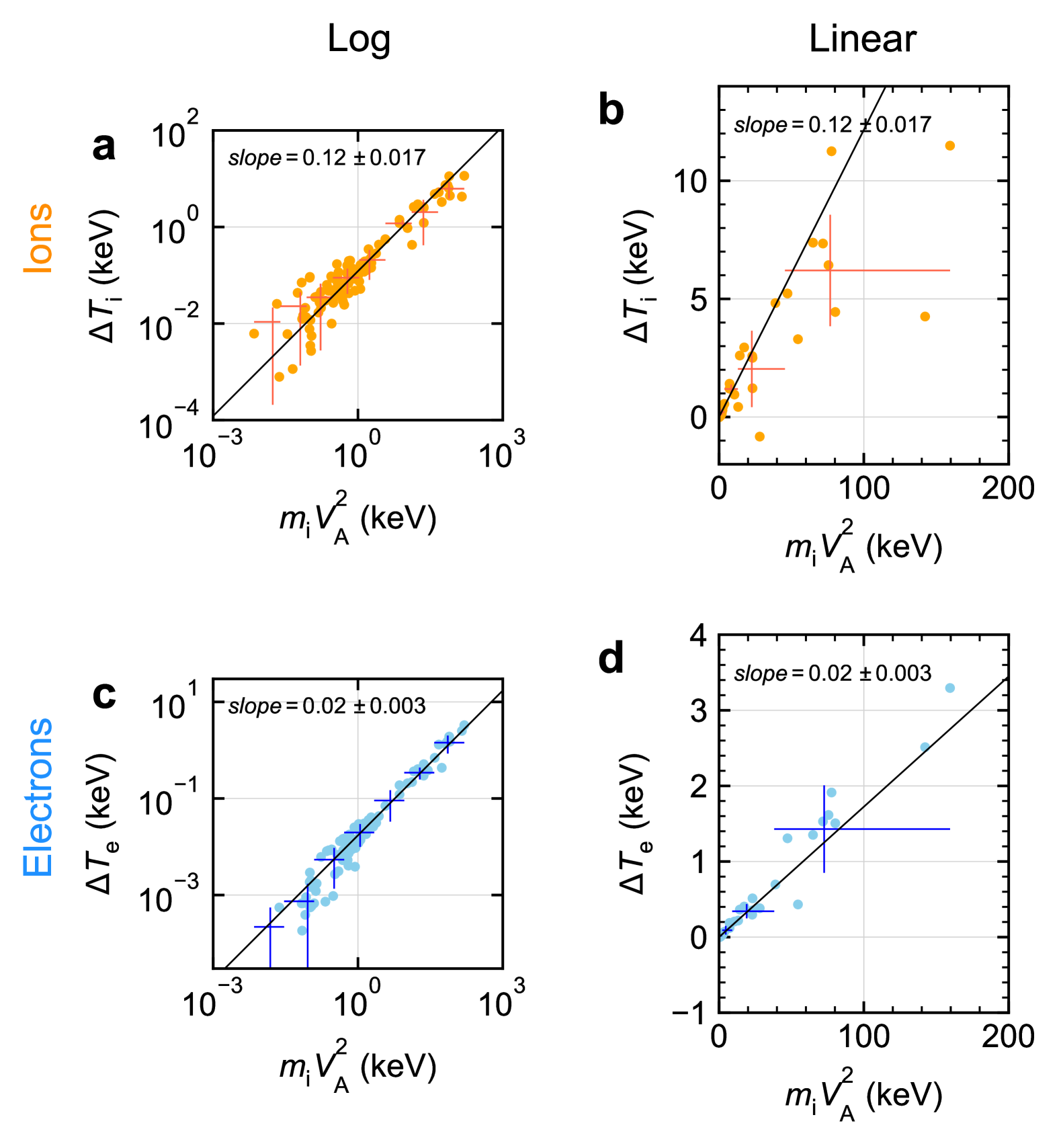
Figure 5: Scaling of particle heating by magnetic reconnection, demonstrating a linear dependence on $m_{\rm i}V_{\rm A}^{2}$ for ions (upper panels) and electrons (lower panels). A linear regression is performed to derive the slope, as annotated on the top left corner of each panel. The same data points and the linear regression results are shown in logarithmic (left panels) and linear (right panels) scales.

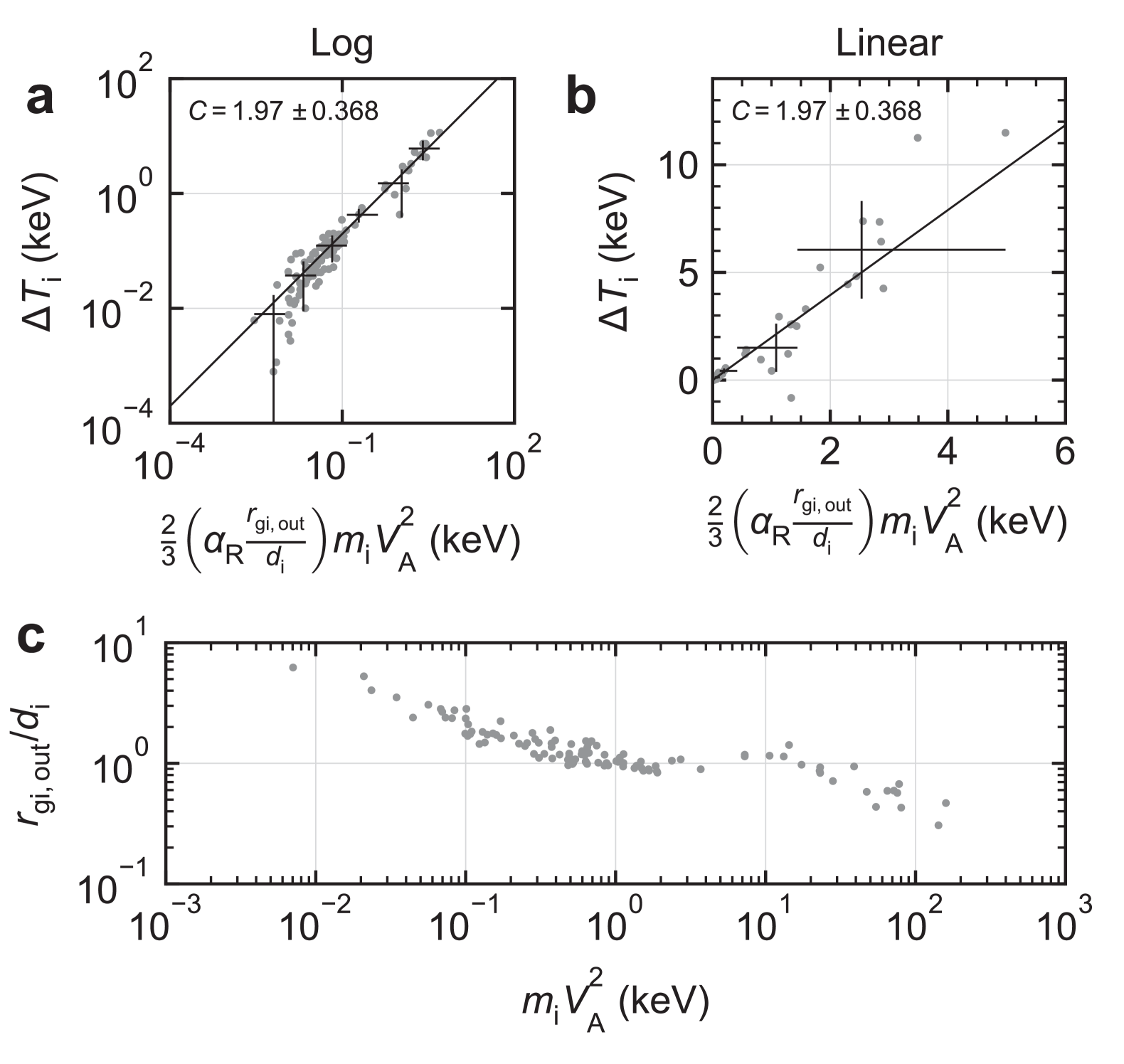
Figure 6: Additional analysis of ion temperature increase and ion gyro-radius during magnetic reconnection. (a) A comparison between the ion temperature increase and the formula based on Eq.(9) with $L=Cr_{\rm gi,out}$ and $\alpha_{R}=0.1$, where $C$ is derived from a linear regression. (b) Same as (a) but displayed in linear scale. (c) the ratio of $r_{\rm gi,out}/d_{\rm i}$ as a function $m_{\rm i}V_{\rm A}^{2}$, demonstrating that $r_{\rm gi,out}$ and $d_{\rm i}$ are often comparable to each other in Earth’s magnetotail reconnection.

Furthermore, we can examine the temperature ratio $\Delta T_{\rm i}/\Delta T_{\rm e}$. Based on Eq.(9) with $L=2d_{\rm i}$ for ion heating and $L=2\sqrt{d_{\rm i}d_{\rm e}}$ for electron heating, we obtain

$$\frac{\Delta T_{i}}{\Delta T_{e}}=\left(\frac{m_{\rm i}}{m_{e}}\right)^{\frac{1}{4}}\sim 6.55$$ (12)

This does not depend on the reconnection rate $\alpha_{\rm R}$ and could provide a universal upper limit to this heating ratio. Figure 7 shows the observed $\Delta T_{\rm i}$ versus $\Delta T_{\rm e}$ (filled circles) as well as the relation obtained from the derived formulas (thin line). It is evident that the prediction of the model matches well with the observed temperature ratios.

If we assume $\Delta T_{i}/\Delta T_{e}\sim T_{i}/T_{e}$, our predicted ratio is within the range of empirically known values of $T_{\rm i}/T_{\rm e}\sim 2-10$ (e.g. SlavinJA_1985_ISEE; BaumjohannW_1989_Average; WangCP_2012_Spatial; WatanabeK_2019_Statistical). It is interesting that a theoretical study of particle motion in a modeled magnetotail predicts $T_{\rm i}/T_{\rm e}\propto(m_{\rm i}/m_{\rm e})^{1/3}$ (SchriverD_1998_origin). Also, a more recent theoretical study based on effective ohmic heating predicts a similar scaling as ours, $\Delta T_{\rm i}/\Delta T_{\rm e}=(m_{\rm i}T_{\rm i0}/m_{\rm e}T_{\rm e0})^{1/4}\sim(m_{\rm i}/m_{\rm e})^{1/4}$, where $T_{\rm i0}$ and $T_{\rm e0}$ are the ion and electron temperature in the plasma sheet before reconnection onset (HoshinoM_2018_Energy).

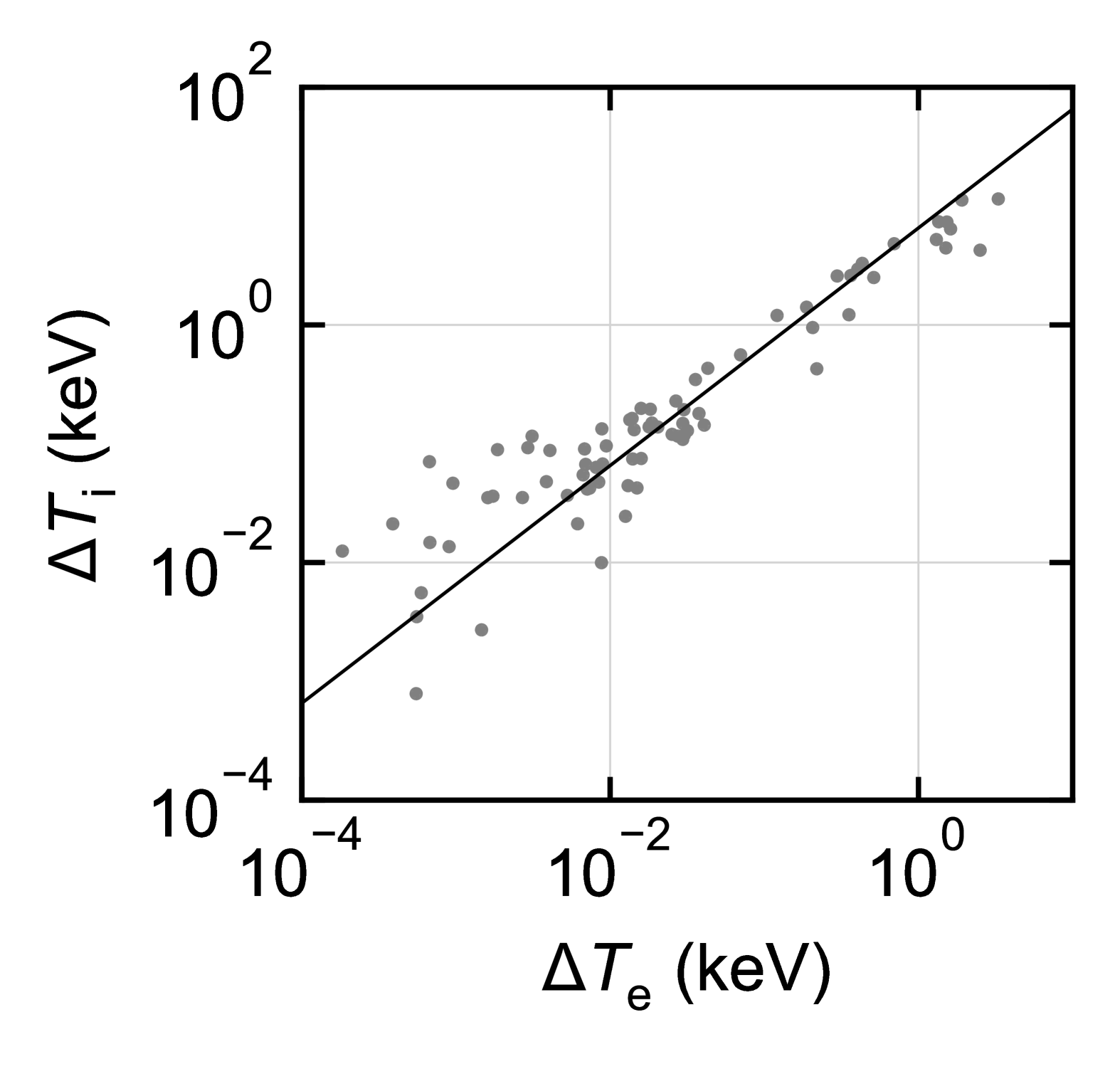
Figure 7: Comparison between ion and electron temperature changes across magnetic reconnection, demonstrating a reasonable match between observations (filled circles) and the model prediction (the black line with a slope of $\sim$6.55).

5 Summary and Discussion

Table 2: Scaling of particle heating derived in this study

	$\displaystyle\Delta T_{\rm i}$	$\displaystyle\Delta T_{\rm e}$	$\displaystyle\frac{\Delta T_{\rm i}}{\Delta T_{\rm e}}$
Shock	43MA(