Supplementary Information
Steric Engineering of Exciton Fine Structure in 2D Perovskites

SUPPLEMENTARY FIGURES

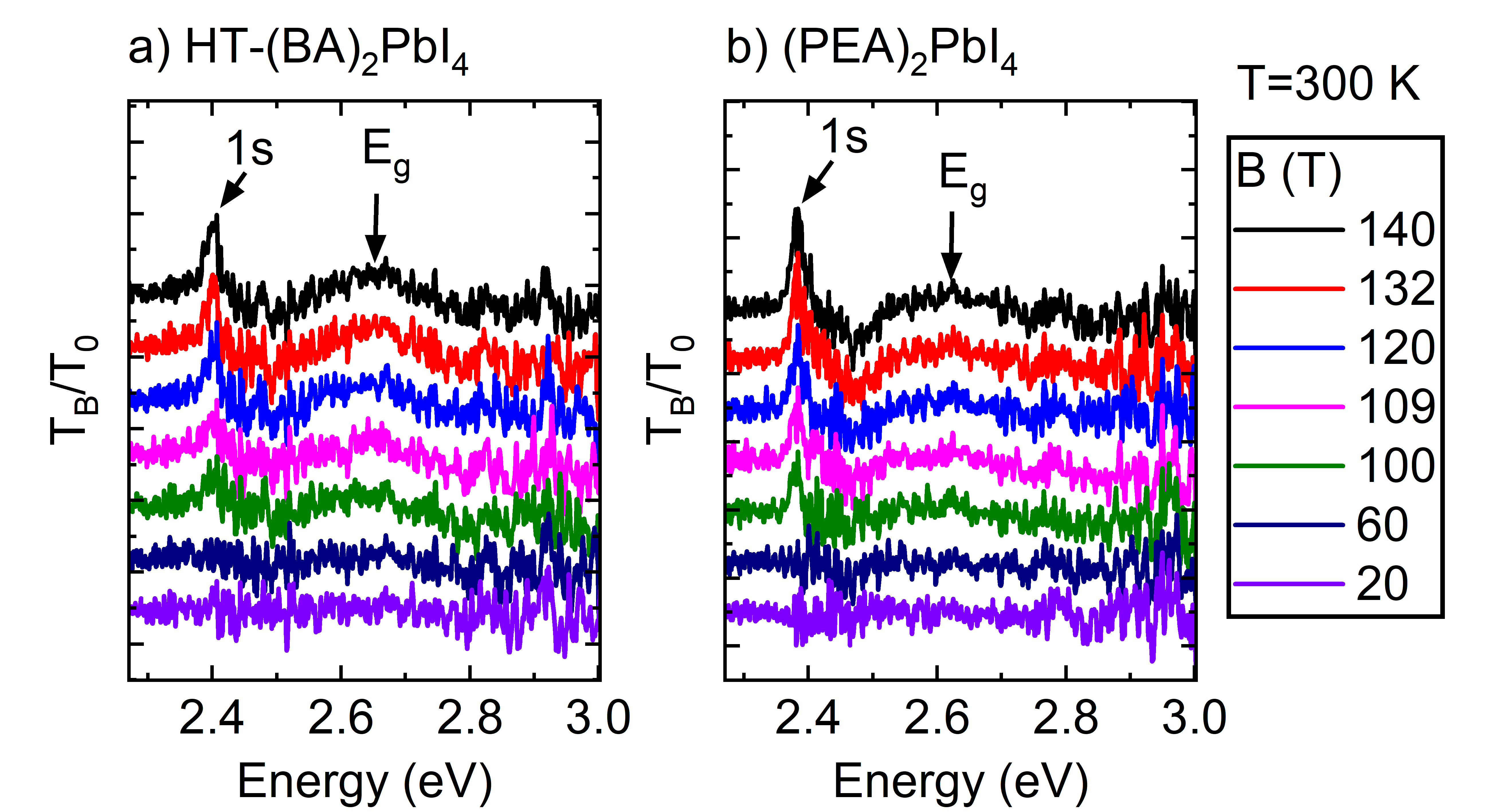
Figure S1: Band gap energy of HT (BA)₂PbI₄ determined from spectroscopy at MegaGauss magnetic fields.
a) Transmission ratio spectra of HT (BA)₂PbI₄ for selected magnetic field strengths. The signal due to band gap E_g and 1s exciton is indicated by arrows. b) For reference, the same experiment is performed on an analogous sample (PEA)₂PbI₄, for which both energies are known[1, 2]

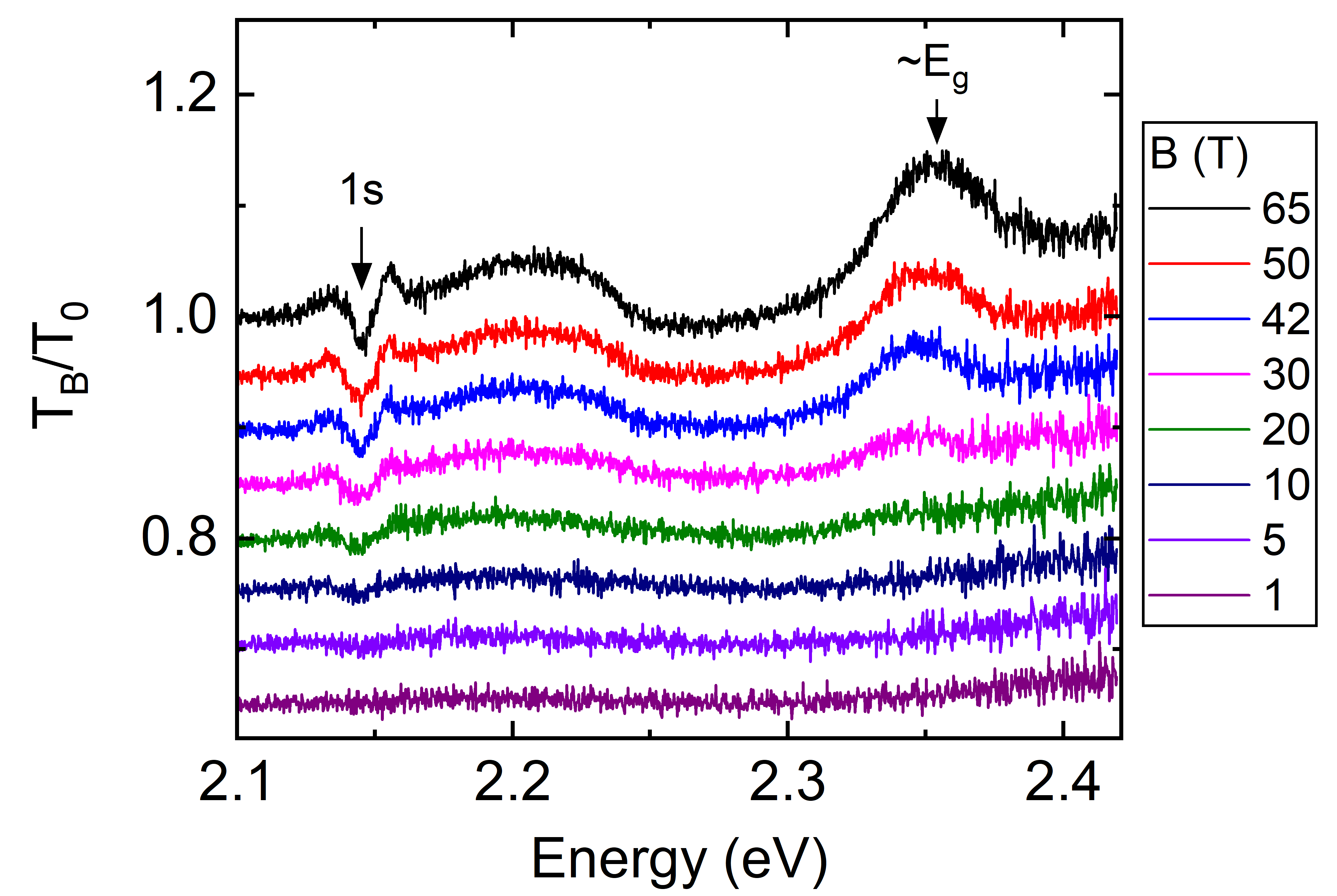
Figure S2: Band gap of (BA)₂SnI₄.
Transmission ratio spectra of (BA)₂SnI₄ for selected magnetic field strengths. The band gap energy E_g and 1s exciton energy are indicated by arrows.

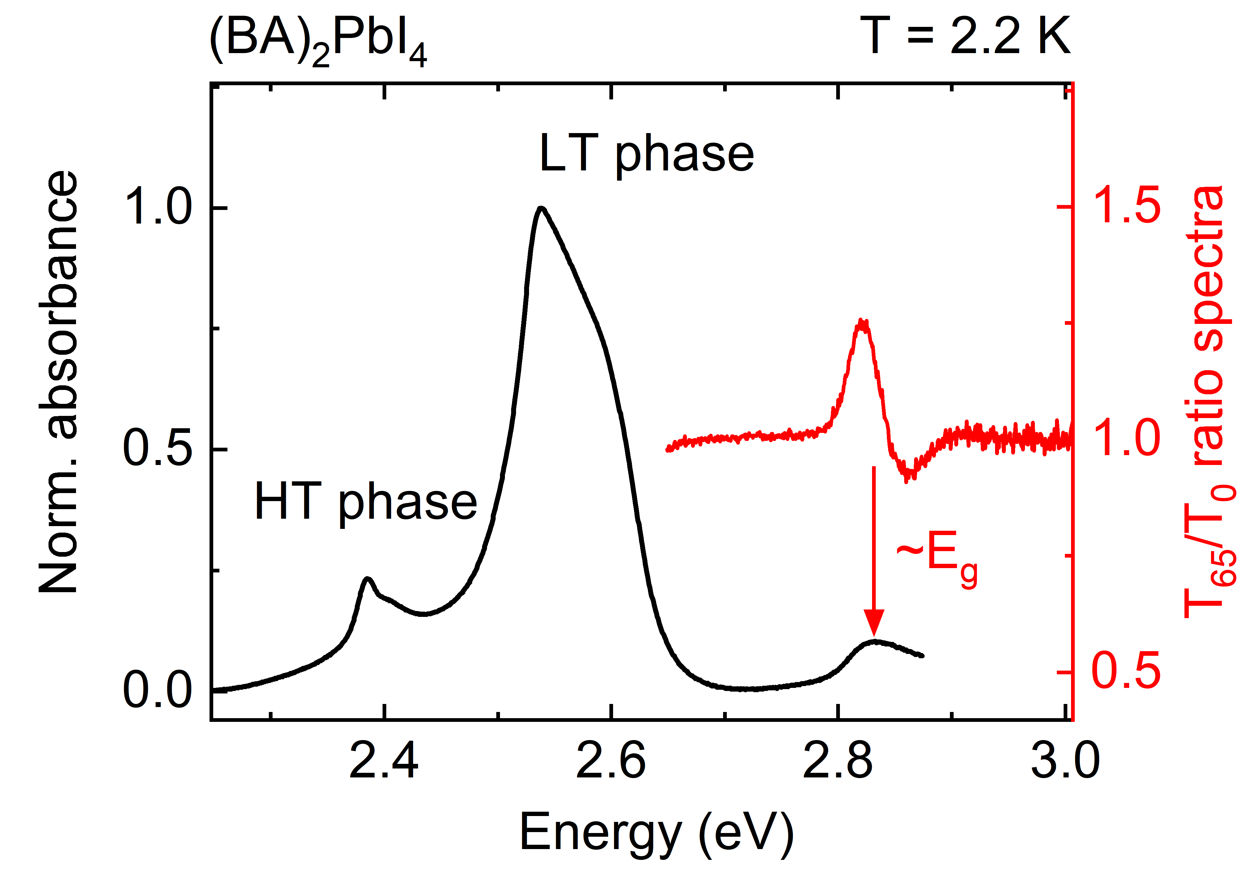
Figure S3: Low temperature spectra of (BA)₂PbI₄.
Low-temperature absorbance spectra of (BA)₂PbI₄ showing the signal due to both HT and LT phases. In red the transmission ratio spectrum is shown (transmission measured at B=65 T divided by zero-field spectrum) in the spectral range of E_g. A clear resonance is observed, allowing for the quasi-particle band gap determination.

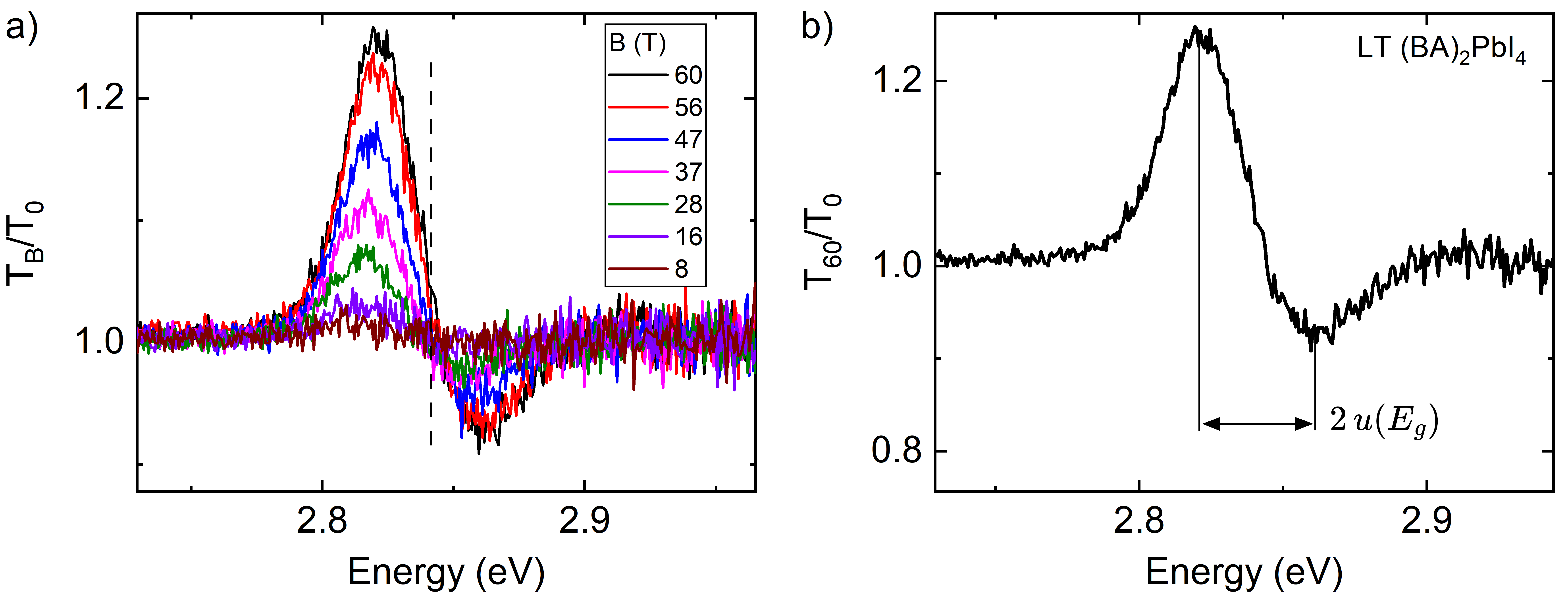
Figure S4: Determination of band gap energy and its uncertainty from the ratio spectrum.
a) Transmission ratio spectrum of LT (BA)₂PbI₄ (transmission measured in the magnetic field divided by zero-field spectrum) for selected field strengths, in the spectral range of the band gap energy E_g. The inflection point, indicated by dashed line, approximates the band gap energy. b) The uncertainty u(E_g) is determined as in the Figure. The same approach is used for other samples studied in the current work, summarized in Table LABEL:Otab:tab2 of the main text.

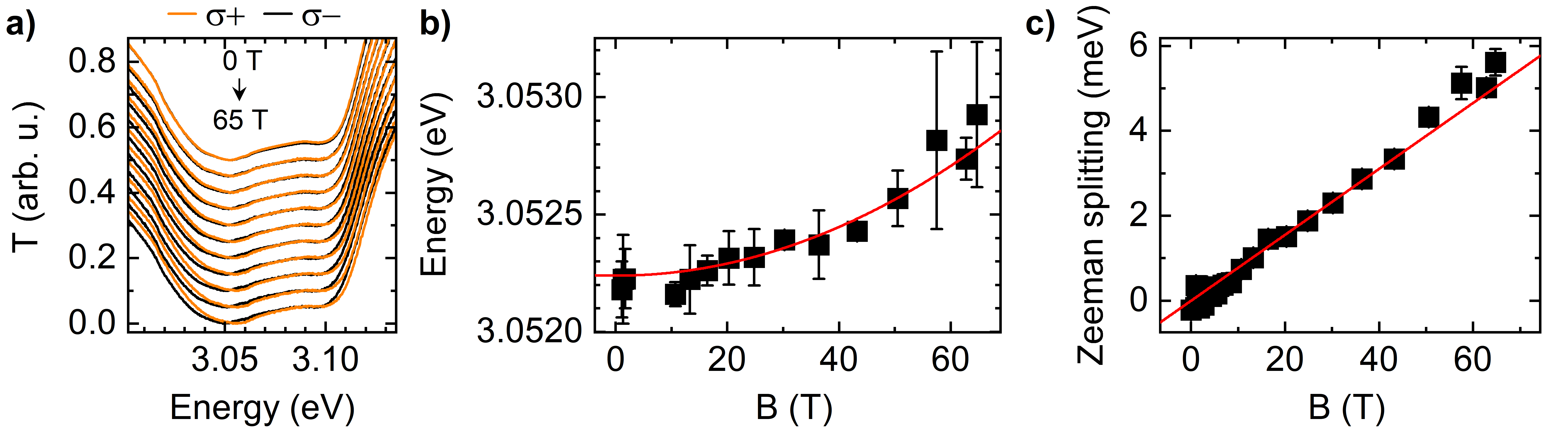
Figure S5: Diamagnetic shift in (PEA)₂PbBr₄.
a) Transmission spectra of (PEA)₂PbBr₄ measured for two circular polarizations $\sigma+$ and $\sigma-$ for selected strengths of magnetic field. b) The energy shift $\Delta E_{1s}=\frac{E_{\sigma+}+E_{\sigma-}}{2}$ of the 1s exciton ($\simeq 3.05$ eV) in the function of magnetic field. Solid line stand for $\Delta E_{1s}=c_{0}B^{2}$. The fitting yields $c_{0}=$0.13\pm 0.02\text{\,}\mathrm{\SIUnitSymbolMicro eV}\text{\,}{\mathrm{T}}^{-2}$$. c) Zeeman splitting with a $g$-factor of $1.3\pm 0.1$.

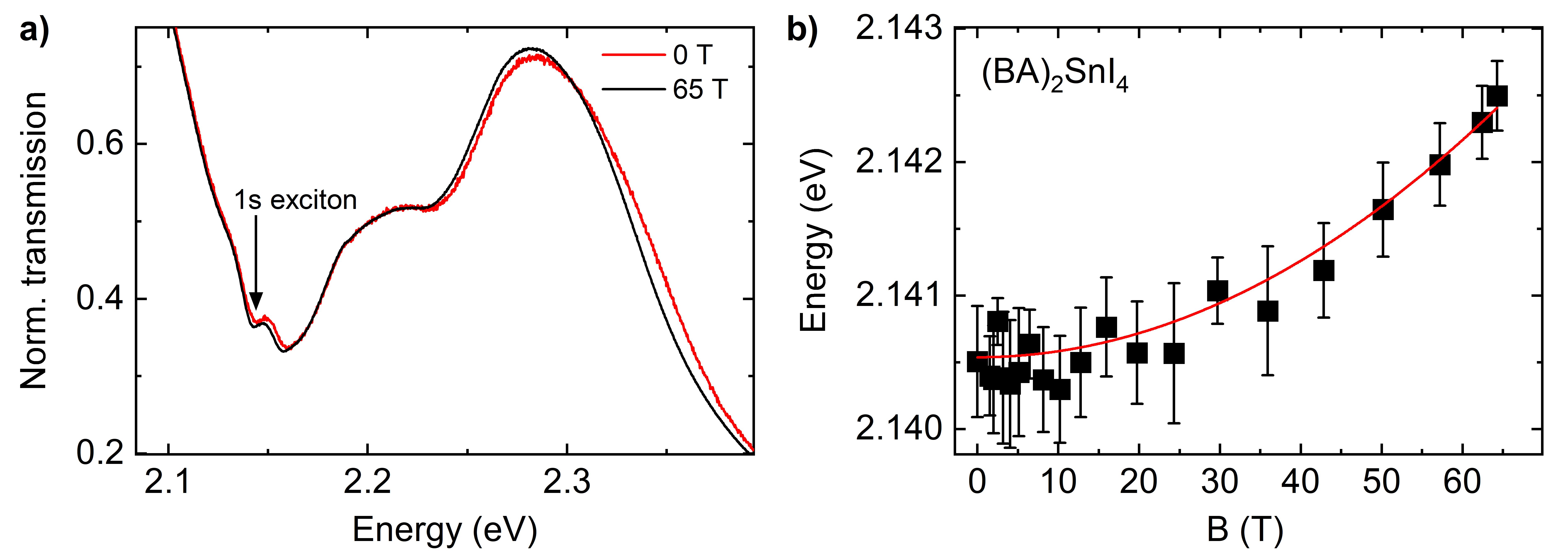
Figure S6: Diamagnetic shift in (BA)₂SnI₄.
a) Transmission spectra of (BA)₂SnI₄ measured at $0$ and $65\text{\,}\mathrm{T}$. b) The energy shift $\Delta E_{1s}$ of 1s exciton in the magnetic field. Solid line stand for $\Delta E_{1s}=c_{0}B^{2}$ dependence. The determined c₀ equals to $0.45\pm 0.03\text{\,}\mathrm{\SIUnitSymbolMicro eV}\text{\,}{\mathrm{T}}^{-2}$

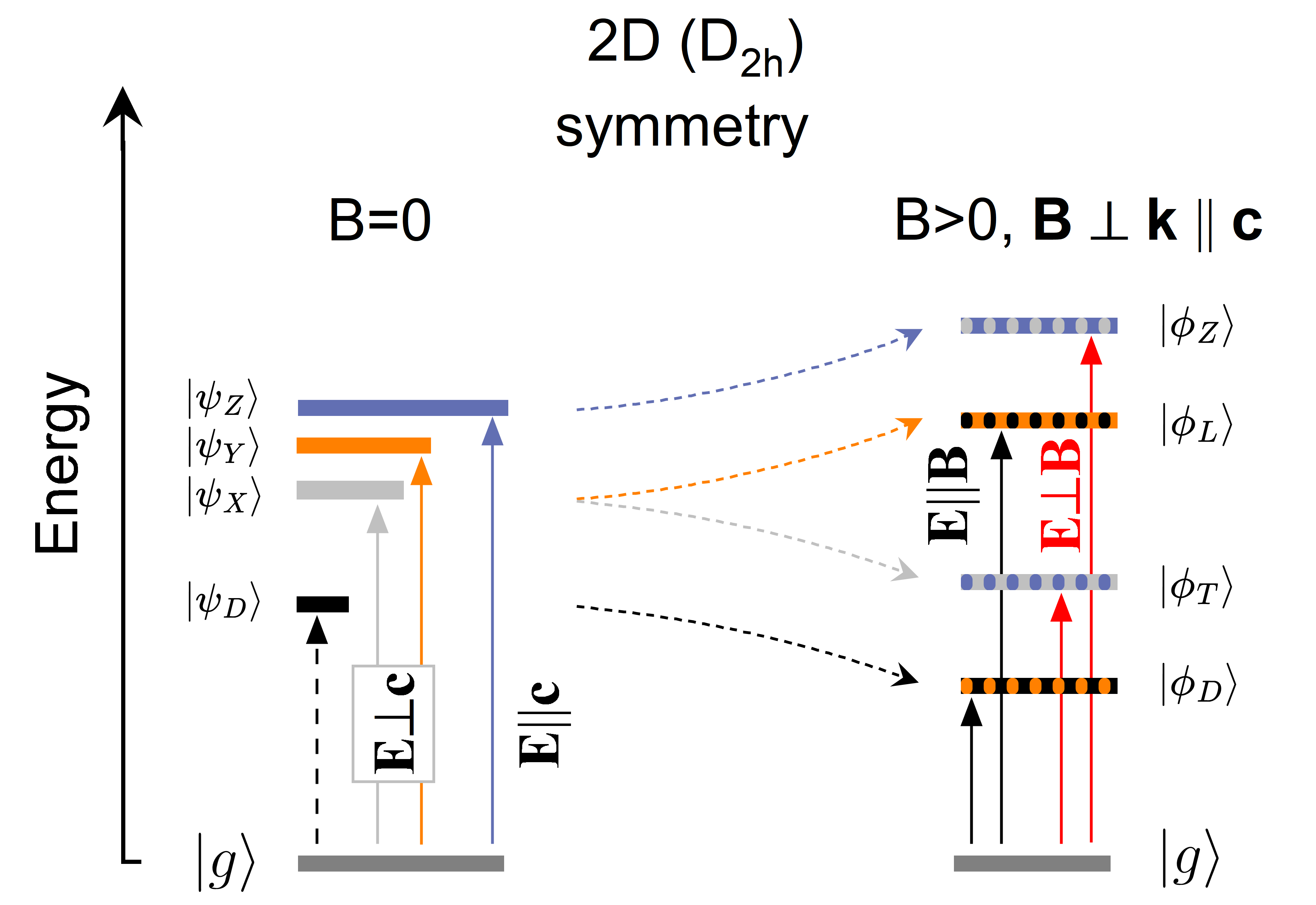
Figure S7: Fine structure splitting of the band-edge excitons for 2D (D${}_{2\textrm{h}}$) symmetry.
The optical selection rules, allowing to access the respective states, are indicated (E is light electric field vector and c is the crystallographic axis perpendicular to quantum well slab). At $B=0$ T (left panel), $|g\rangle$ - the ground state (no exciton); $|\psi_{D}\rangle$ - dark state. The $|\psi^{X}\rangle$ and $|\psi^{Y}\rangle$ are bright states with in-plane dipole moment and $|\psi_{Z}\rangle$ state is a bright state with out-of-plane dipole moment. At $B>0$ and $\mathbf{B}\perp\mathbf{k}\parallel\mathbf{c}$ (right panel) all four states ($|\phi_{D}\rangle$, $|\phi_{Z}\rangle$, $|\phi_{L}\rangle$, $|\phi_{T}\rangle$) have nonzero dipole moment in the plane of 2D perovskite.

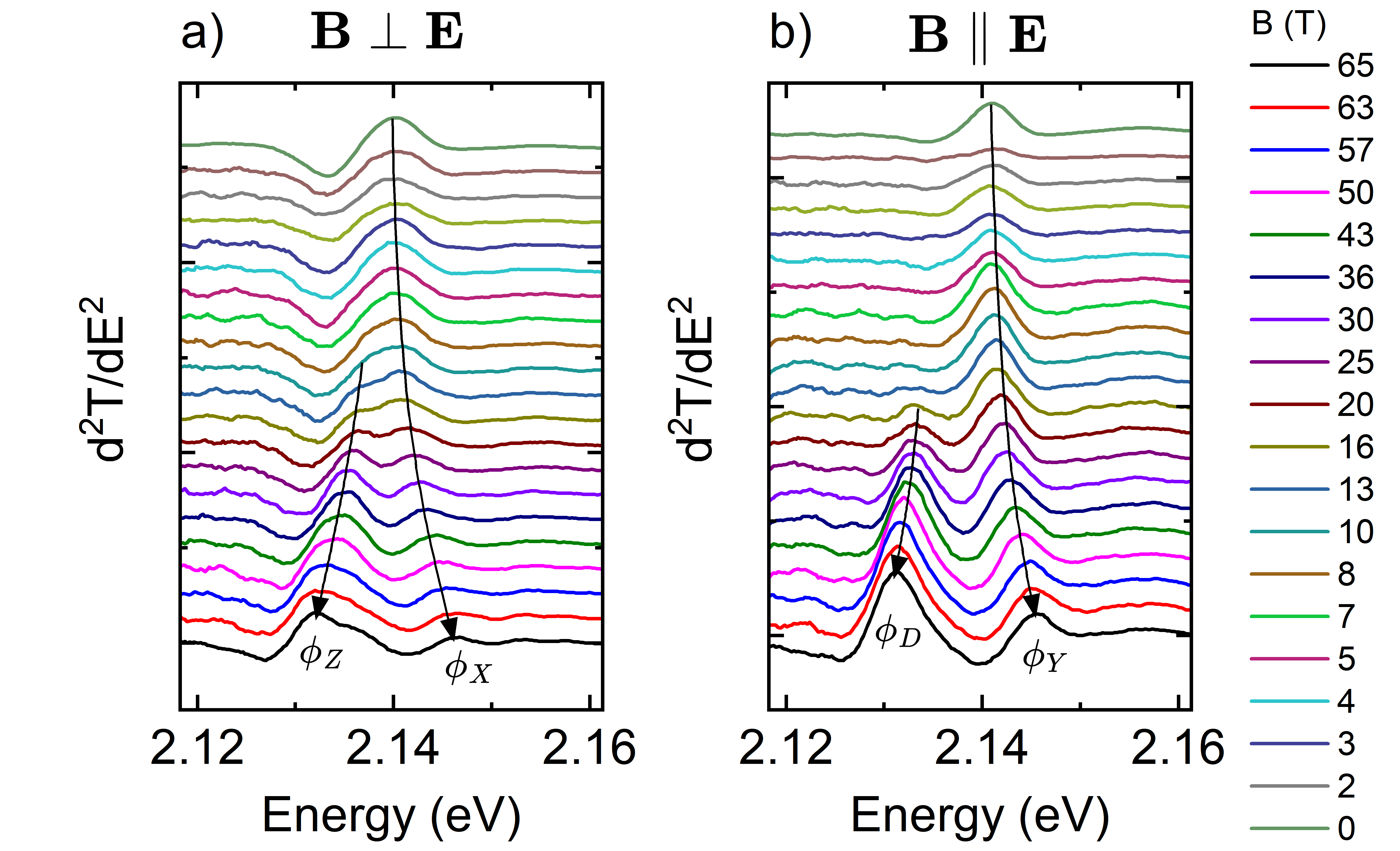
Figure S8: Transmission of (BA)₂SnI₄ in Voigt geometry.
2nd derivative of transmission of (BA)₂SnI₄ measured in Voigt geometry for several magnetic field strengths for a) $\textbf{B}\perp\textbf{E}$ and b) $\textbf{B}\parallel\textbf{E}$ configurations. In the high magnetic field (bottom curves) all four excitonic states are observed.

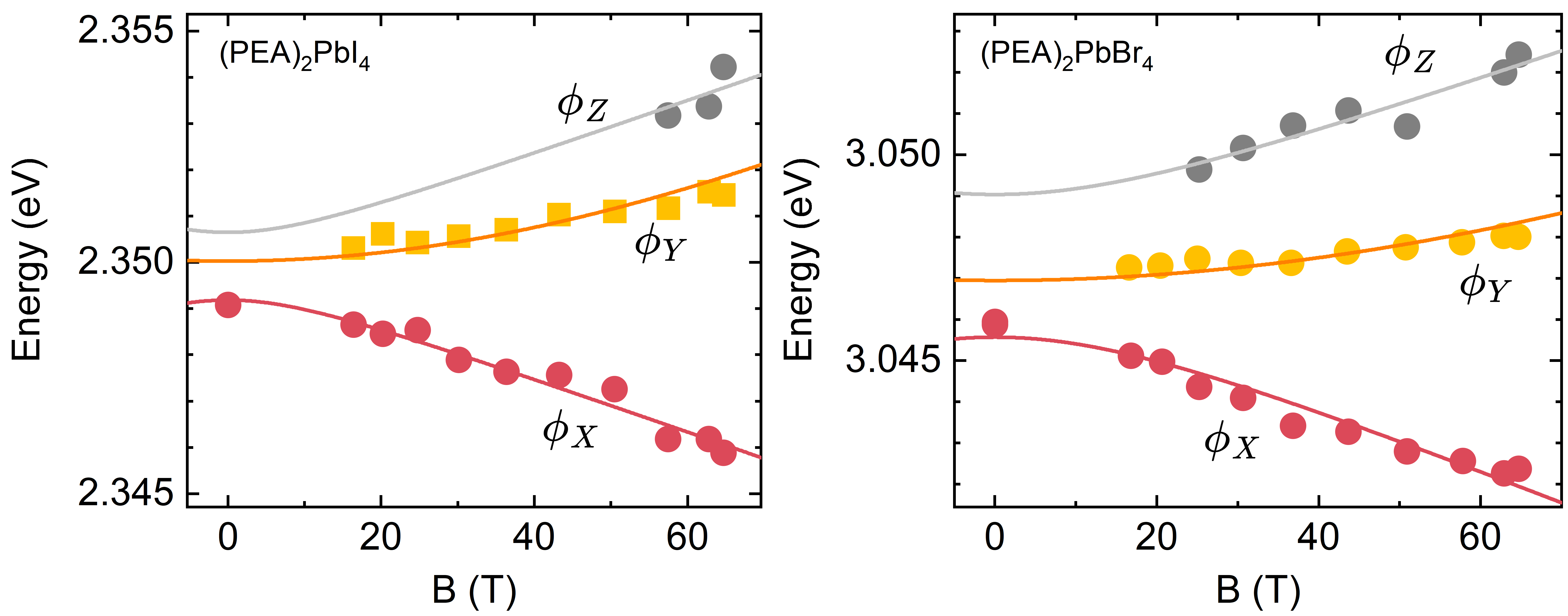
Figure S9: The energy shift of bright excitons in (PEA)₂PbI₄ and (PEA)₂PbBr₄
The evolution of optical transition energy for three bright states of (PEA)₂PbI₄ and (PEA)₂PbBr₄. Solid lines stand for fits with eq. LABEL:Oeq:shift1-LABEL:Oeq:shift2 of the main text.

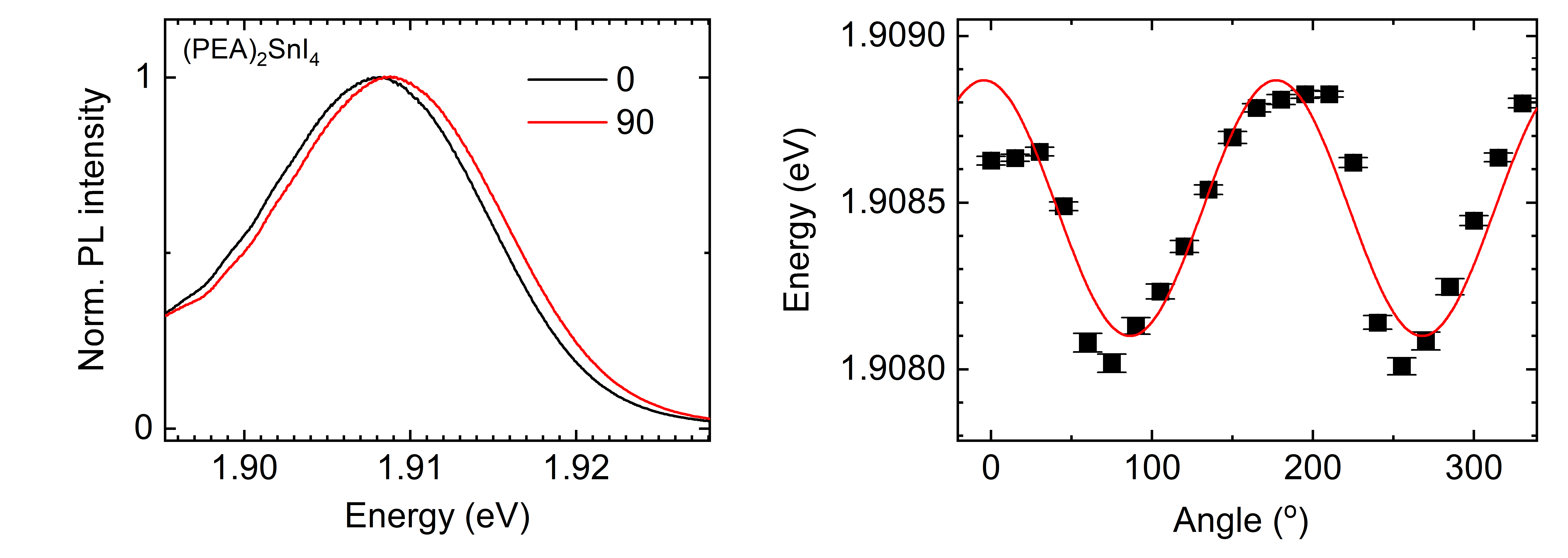
Figure S10: $\Delta_{XY}$ in (PEA)₂SnI₄.
In order to approximate the energy splitting between the bright in-plane states of (PEA)₂SnI₄ we performed photoluminescence (PL) measurements in the linear basis at T=$4.2\text{\,}\mathrm{K}$. a) The PL spectra for two orthogonal polarizations. A clear difference between the $0\text{\,}\mathrm{\SIUnitSymbolDegree}$ and $90\text{\,}\mathrm{\SIUnitSymbolDegree}$ curves is visible. b) The PL peak energy in the function of polarization angle. The solid line is a cosine fit, yielding the $\Delta_{XY}$=$0.77\pm 0.1\text{\,}\mathrm{m}\mathrm{eV}$.

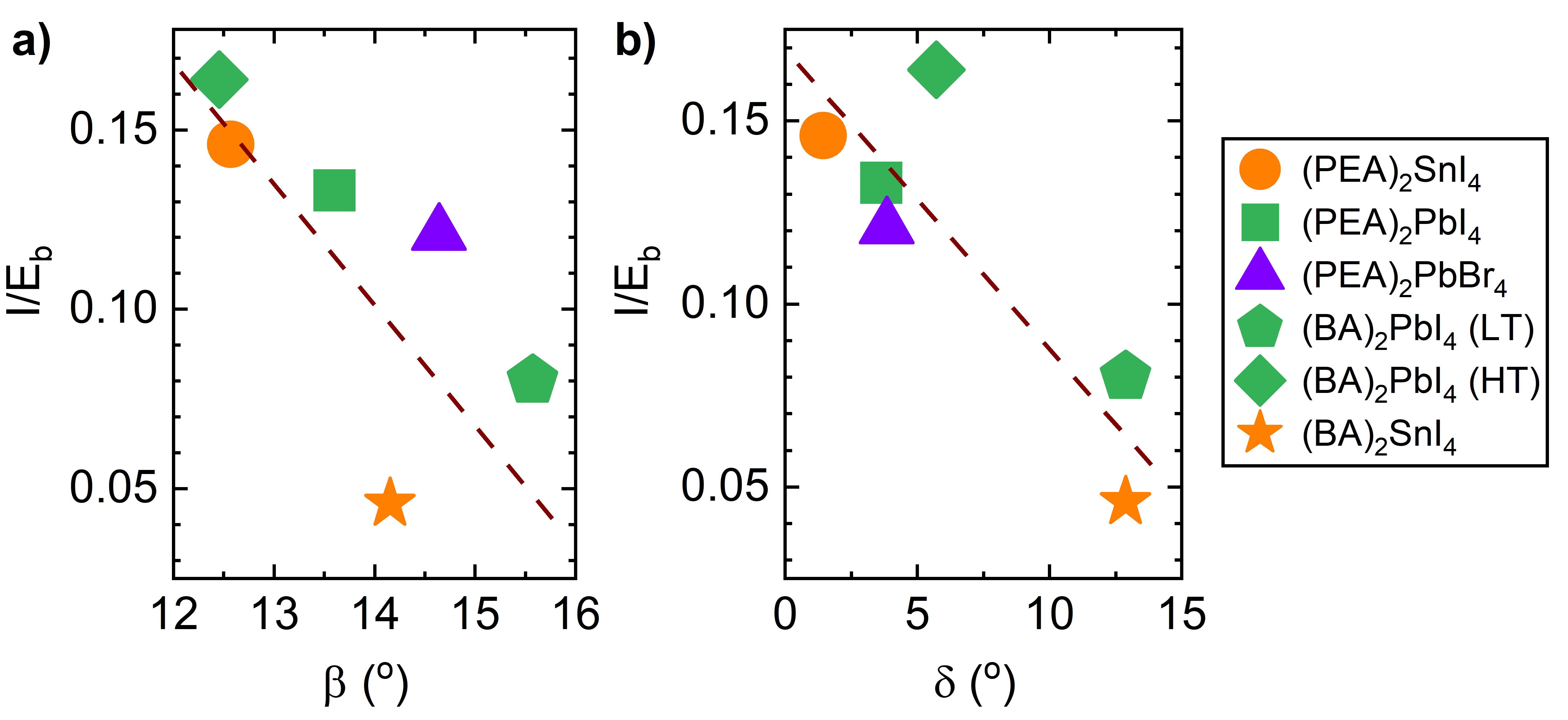
Figure S11: I/E_b ratio in the function of $\beta$ and $\delta$ distortion angles.
The ratio of the exchange energy $I$ and exciton binding energy E_b in the function of a) in-plane distortion angle $\beta$ and b) out-of-plane corrugation angle $\delta$. The figure serves as a support to Figure LABEL:Ofig:fig5_theory of the main text, where I/E_b is plotted in the function of $\beta+\delta$. The dashed lines are guides to the eye.

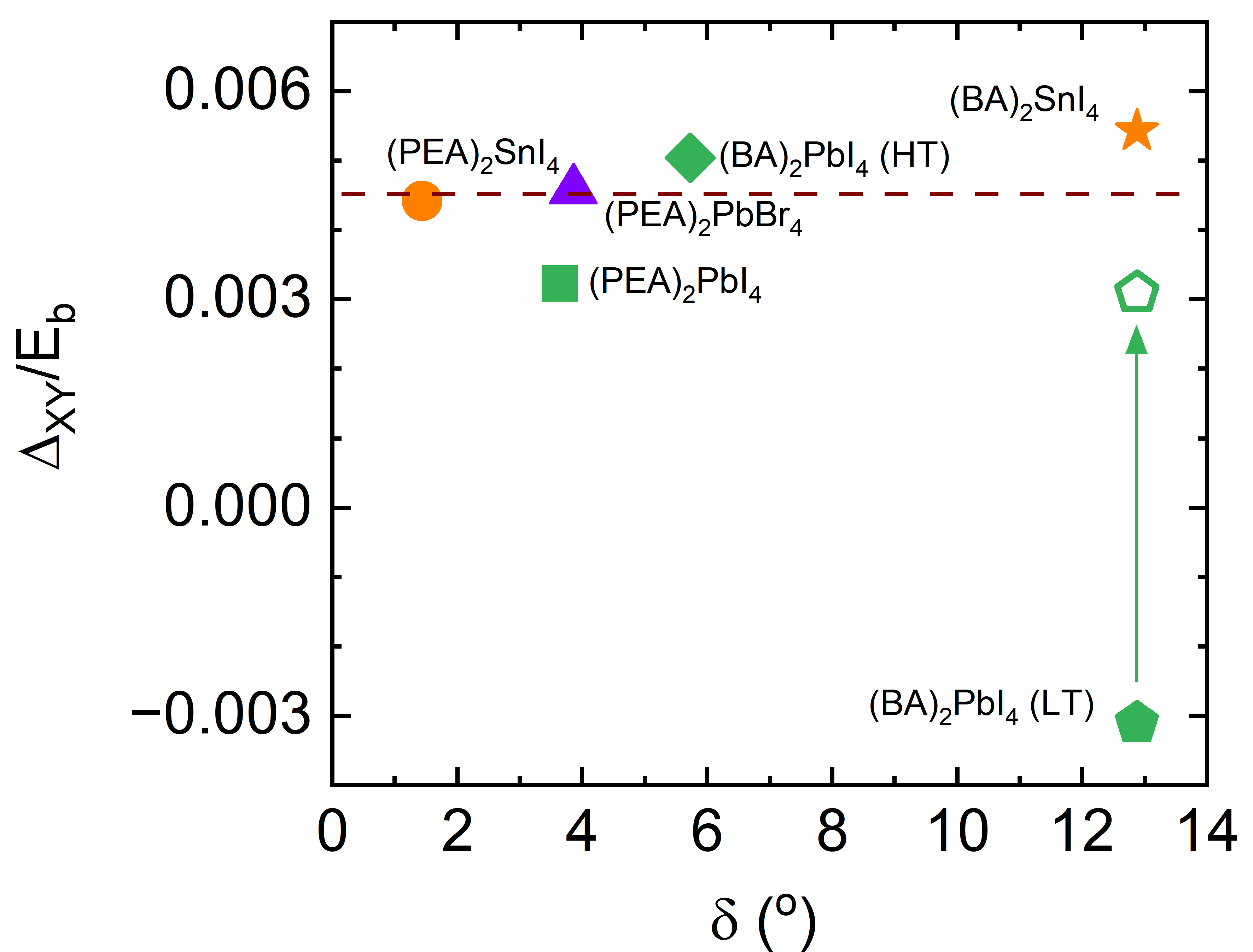
Figure S12: Impact of corrugation on the bright-bright splitting.
The ratio of the energy splitting between the bright in-plane excitons $\Delta_{XY}$ and exciton binding energy E_b in the function of out-of-plane corrugation $\delta$. The open symbol stands for the absolut $\Delta_{XY}$ value for LT (BA)₂PbI₄.

SUPPLEMENTARY TABLES

Table S1: Summary of $g$-factor measured in Voigt geometry. From the left: effective $g$-factors for longitudinal ($g_{L}=g_{e\perp}-g_{h\perp}$) and transverse ($g_{T}=g_{e\perp}+g_{h\perp}$) states, individual electron $g_{e\perp}$ and hole $g_{h\perp}$ $g$-factors both defined for the direction normal to the B vector.

	$g_{L}$	$g_{T}$	$g_{e\perp}$	$g_{h\perp}$
(BA)2SnI4 - LT	$3.3\pm 0.3$	$3.8\pm 0.1$	$3.5\pm 0.4$	$0.26\pm 0.32$
(BA)2PbI4 - LT	$2.7\pm 0.5$	$2.9\pm 0.1$	$2.8\pm 0.6$	$0.10\pm 0.51$
(BA)2PbI4 - HT	$3.3\pm 0.2$	$1.8\pm 0.1$	$2.6\pm 0.3$	$-0.7\pm 0.3$
(PEA)2PbI4	$3.6\pm 0.3$	$2.0\pm 0.2$	$2.8\pm 0.4$	$-0.79\pm 0.36$
(PEA)2PbBr4	$3.5\pm 0.3$	$2.8\pm 0.2$	$3.1\pm 0.4$	$-0.35\pm 0.36$

Table S2: Effective mass of charge carriers
The effective mass of charge carriers $\mu$ used to estimate the 1s exciton rms radius in Figure LABEL:Ofig:fig6_bohr_radius of the main text. The $\mu$ for (PEA)₂PbI₄ is measured from the Landau level spectroscopy[2]. The $\mu$ for other compounds is approximated from a phenomenological scaling law[3].

	$\mu(\unit{m_{0}})$
(PEA)2PbI4	0.087[2]
(PEA)2SnI4	0.072
(PEA)2PbBr4	0.155
(BA)2SnI4	0.083
(BA)2PbI4 - LT	0.126
(BA)2PbI4 - HT	0.089

Microscopic model of exciton fine structure

The orbital wavefunctions can be be decomposed into their individual contributions, determined by the spin-orbit coupling. The latter leads to a mixing of the orbital composition of the lowest conduction band [4] with momentum $k$, spin $s$ and orbital $P_{i}$

$$\ket{s,c,k}=a_{z}\sigma_{s}\ket{P_{z},s,k}+a_{x}\ket{P_{x},\overline{s},k}+ia_{y}\sigma_{s}\ket{P_{y},\overline{s},k},$$ (1)

where $\sigma=\pm 1$ denotes the up/down spin, respectively. Here $a_{i}$ determines the contribution of the orbital $P_{i}$ to the valence band. Equal weighting of the $P_{x}$, $P_{y}$ and $P_{z}$ orbitals corresponds to a perovskite with cubic symmetry ($a_{x}=a_{y}=a_{z}=\frac{1}{\sqrt{3}}$). In the orthorhombic phase the weightings differ [5], however the contributing orbitals remain the same. In particular, $a_{x}=a_{y}=\dfrac{1}{\sqrt{2}}\cos\theta$ and $a_{z}=\sin\theta$ where $\theta$ is a material specific parameter. There is no mixing of the valence band $S$ orbitals in any phase. The exchange Hamiltonian can be written as a 4x4 matrix describing each spin state [6]. As such we need to solve the eigenproblem

$$\begin{pmatrix}a_{z}^{2}I_{z}&0&0&-a_{z}^{2}I_{z}\\ 0&a_{x}^{2}I_{x}+a_{y}^{2}I_{y}&a_{x}^{2}I_{x}-a_{y}^{2}I_{y}&0\\ 0&a_{x}^{2}I_{x}-a_{y}^{2}I_{y}&a_{x}^{2}I_{x}+a_{y}^{2}I_{y}&0\\ -a_{z}^{2}I_{z}&0&0&a_{z}^{2}I_{z}\\ \end{pmatrix}\begin{pmatrix}D^{\uparrow,\uparrow,n}\\ D^{\uparrow,\downarrow,n}\\ D^{\downarrow,\uparrow,n}\\ D^{\downarrow,\downarrow,n}\end{pmatrix}=E^{n}\begin{pmatrix}D^{\uparrow,\uparrow,n}\\ D^{\uparrow,\downarrow,n}\\ D^{\downarrow,\uparrow,n}\\ D^{\downarrow,\downarrow,n},\end{pmatrix}$$ (2)

where $I_{x,y,z}$ are the exchange integrals for the $P_{x}$, $P_{y}$ and $P_{z}$ orbitals respectively. Here $D^{\uparrow,\uparrow,n}$ describes the spin contribution to each exciton band $n$ with energy $E^{n}$. For the tetragonal system $a_{x}=a_{y}$ and $I_{x}=I_{y}$ and leading to the energy landscape

$$E^{0} =0\quad\text{(dark)}$$

$$E^{1} =2a_{x}^{2}I_{x}\quad\text{(LCP)}$$

$$E^{2} =2a_{x}^{2}I_{x}\quad\text{(RCP)}$$

$$E^{3} =2a_{z}^{2}I_{z}\quad\text{(Z)}$$

In contrast, if $a_{x}\neq a_{y}$ or $I_{x}\neq I_{y}$ we have

$$E^{0} =0\quad\text{(dark)}$$

$$E^{1} =2a_{x}^{2}I_{x}\quad\text{(X)}$$

$$E^{2} =2a_{y}^{2}I_{y}\quad\text{(Y)}$$

$$E^{3} =2a_{z}^{2}I_{z}\quad\text{(Z)}$$

The bright-dark splitting as defined here, is the splitting between the bright $X$-polarised exciton ($n=1$) and the dark ($n=0$) exciton, as it is these that mix when a magnetic field is applied. We also know by the normalisation of the wavefucntion that $a_{x}^{2}+a_{y}^{2}+a_{z}^{2}=1$. Assuming that $I_{x}=I_{y}=I_{z}=I$ and that relative orbital contributions to the band dictate the ordering of states, combined with the normalisation condition allows us to extract $I,a_{x,y,z}$ from the equation from the exciton resonances. In particular we solve the system of equations

$$Ia_{x}^{2} =\Delta_{BD}$$

$$I(a_{y}^{2}-a_{z}^{2}) =\Delta_{XY}$$

$$I(a_{z}^{2}-a_{y}^{2}) =\Delta_{BZ}$$

$$a_{x}^{2}+a_{y}^{2}+a_{z}^{2} =1,$$

in order to uniquely determine $I,a_{x,y,z}$ as discussed in the main text.

The impact of the magnetic field can be included by considering a new 4x4 Hamiltonian whose basis is the exciton states in the absence of a magnetic field [6]

$$H_{X}(B)=\begin{pmatrix}E_{\text{Dark}}&0&\dfrac{1}{2}g_{L}\mu_{B}B&0\\ 0&E_{\text{Z}}&0&\dfrac{1}{2}g_{T}\mu_{B}B\\ \dfrac{1}{2}g_{L}\mu_{B}B&0&E_{\text{X}}&0\\ 0&\dfrac{1}{2}g_{T}\mu_{B}B&0&E_{\text{Y}}\\ \end{pmatrix}$$ (3)

where $g_{L}=g_{c}-g_{v}$ and $g_{T}=g_{c}+g_{v}$ depend on the g-factors $g_{c(v)}$ of the exciton-weighted electron (hole) bands [6]. Solving the matrix above, we obtain the eigenvalues

$$E_{0L}(B)=\dfrac{1}{2}\left(E_{\text{Dark}}+E_{\text{X}}+\sqrt{(E_{\text{Dark}}-E_{\text{X}})^{2}+(g_{L}\mu_{B}B)^{2}}\right)$$ (4)

$$E_{1L}(B)=\dfrac{1}{2}\left(E_{\text{Dark}}+E_{\text{X}}-\sqrt{(E_{\text{Dark}}-E_{\text{X}})^{2}+(g_{L}\mu_{B}B)^{2}}\right)$$ (5)

$$E_{0T}(B)=\dfrac{1}{2}\left(E_{\text{Y}}+E_{\text{Z}}-\sqrt{(E_{\text{Y}}-E_{\text{Z}})^{2}+(g_{T}\mu_{B}B)^{2}}\right)$$ (6)

$$E_{1T}(B)=\dfrac{1}{2}\left(E_{\text{Y}}+E_{\text{Z}}+\sqrt{(E_{\text{Y}}-E_{\text{Z}})^{2}+(g_{T}\mu_{B}B)^{2}}\right)$$ (7)

The corresponding eigenstates are

$$\psi_{0L}(B)=\dfrac{2}{\sqrt{\mathcal{N}}}\begin{pmatrix}\dfrac{E_{0L}(B)-E_{X}}{g_{L}\mu_{B}B/2}\\ 0\\ 1\\ 0\end{pmatrix}$$ (9)

$$\psi_{1L}(B)=\dfrac{2}{\sqrt{\mathcal{N}}}\begin{pmatrix}\dfrac{E_{1L}(B)-E_{X}}{g_{L}\mu_{B}B/2}\\ 0\\ 1\\ 0\end{pmatrix}$$ (10)

$$\psi_{0T}(B)=\dfrac{2}{\sqrt{\mathcal{N}}}\begin{pmatrix}0\\ \dfrac{E_{0T}(B)-E_{Y}}{g_{T}\mu_{B}B/2}\\ 0\\ 1\end{pmatrix}$$ (11)

$$\psi_{1T}(B)=\dfrac{2}{\sqrt{\mathcal{N}}}\begin{pmatrix}0\\ \dfrac{E_{1T}(B)-E_{Y}}{g_{T}\mu_{B}B/2}\\ 0\\ 1\end{pmatrix}$$ (12)

References

- Dyksik et al. [2020] M. Dyksik, H. Duim, X. Zhu, Z. Yang, M. Gen, Y. Kohama, S. Adjokatse, D. K. Maude, M. A. Loi, D. A. Egger, et al., Broad tunability of carrier effective masses in two-dimensional halide perovskites, ACS Energy Letters 5, 3609 (2020).
- Dyksik et al. [2021] M. Dyksik, S. Wang, W. Paritmongkol, D. K. Maude, W. A. Tisdale, M. Baranowski, and P. Plochocka, Tuning the Excitonic Properties of the 2D (PEA)2(MA)n-1PbnI3n+1 Perovskite Family via Quantum Confinement, The Journal of Physical Chemistry Letters 12, 1638 (2021).
- Dyksik [2022] M. Dyksik, Using the Diamagnetic Coefficients to Estimate the Reduced Effective Mass in 2D Layered Perovskites: New Insight from High Magnetic Field Spectroscopy, International Journal of Molecular Sciences 23, 12531 (2022).
- Becker et al. [2018] M. A. Becker, R. Vaxenburg, G. Nedelcu, P. C. Sercel, A. Shabaev, M. J. Mehl, J. G. Michopoulos, S. G. Lambrakos, N. Bernstein, J. L. Lyons, T. Stöferle, R. F. Mahrt, M. V. Kovalenko, D. J. Norris, G. Rainò, and A. L. Efros, Bright triplet excitons in caesium lead halide perovskites, Nature 553, 189 (2018).
- Steger et al. [2022] M. Steger, S. M. Janke, P. C. Sercel, B. W. Larson, H. Lu, X. Qin, V. W.-z. Yu, V. Blum, and J. L. Blackburn, On the optical anisotropy in 2d metal-halide perovskites, Nanoscale 14, 752 (2022).
- Thompson et al. [2024] J. J. P. Thompson, M. Dyksik, P. Peksa, K. Posmyk, A. Joki, R. Perea‐Causin, P. Erhart, M. Baranowski, M. A. Loi, P. Plochocka, and E. Malic, Phonon‐Bottleneck Enhanced Exciton Emission in 2D Perovskites, Advanced Energy Materials 14, 1 (2024), arXiv:2312.10688 .