Bayesian Modeling of Zero-Shot Classifications
for Urban Flood Detection
Abstract.
Street scene datasets, collected from Street View or dashboard cameras, offer a promising means of detecting urban objects and incidents like street flooding. However, a major challenge in using these datasets is their lack of reliable labels: there are myriad types of incidents, many types occur rarely, and ground-truth measures of where incidents occur are lacking. Here, we propose BayFlood, a two-stage approach which circumvents this difficulty. First, we perform zero-shot classification of where incidents occur using a pretrained vision-language model (VLM). Second, we fit a spatial Bayesian model on the VLM classifications. The zero-shot approach avoids the need to annotate large training sets, and the Bayesian model provides frequent desiderata in urban settings — principled measures of uncertainty, smoothing across locations, and incorporation of external data like stormwater accumulation zones. We comprehensively validate this two-stage approach, showing that VLMs provide strong zero-shot signal for floods across multiple cities and time periods, the Bayesian model improves out-of-sample prediction relative to baseline methods, and our inferred flood risk correlates with known external predictors of risk. Having validated our approach, we show it can be used to improve urban flood detection: our analysis reveals 113,738 people who are at high risk of flooding overlooked by current methods, identifies demographic biases in existing methods, and suggests locations for new flood sensors. More broadly, our results showcase how Bayesian modeling of zero-shot LM annotations represents a promising paradigm because it avoids the need to collect large labeled datasets and leverages the power of foundation models while providing the expressiveness and uncertainty quantification of Bayesian models.
1. Introduction
Street scene datasets, derived from dashboard cameras (”dashcams”) or Street View data, offer an unparalleled view into urban life. They have been used to count urban objects, including trees (Berland and Lange, 2017; Li et al., 2018b; Branson et al., 2018), traffic signs (Campbell et al., 2019), curb ramps (Hara et al., 2014) and manholes (Vishnani et al., 2020); measure inequality in policing and surveillance (Franchi et al., 2023; Sheng et al., 2021); estimate demographics (Gebru et al., 2017), pedestrian counts (Yin et al., 2015), safe infrastructure (Rundle et al., 2011), navigability (Yin and Wang, 2016; Franchi, Matt et al., 2025) and gentrification (Ilic et al., 2019); and measure neighborhood changes over time (Naik et al., 2017).
However, a major challenge in using street scene data is acquiring large labeled datasets with which to train computer vision models to detect objects of interest (Rundle et al., 2011). This is challenging for several reasons. First, there are myriad types of objects and incidents we might wish to detect. Past work has studied hundreds of types of urban incidents (Balachandar et al., [n. d.]); thousands of types of vehicles (Gebru et al., 2017); and hundreds of types of trees (Berland and Lange, 2017). Each of these types necessitates its own labels. A second challenge is that many types of urban phenomena appear rarely — for example, street flooding occurs infrequently and does not affect most streets — creating a class imbalance problem which can make it challenging to curate sufficient positive examples with which to train and evaluate a model. A final obstacle is that ground-truth for many urban phenomena is difficult to obtain: for example, resident reporting systems identifying where urban problems occur are noisy and have demographic biases (Agostini et al., 2024; Kontokosta and Hong, 2021; McLafferty et al., 2020; Balachandar et al., [n. d.]; Liu and Garg, 2024; Liu et al., 2024a).
Because obtaining large labeled datasets is challenging, an appealing solution is to instead perform zero-shot classification using pretrained vision-language models (VLMs): for example, by prompting the model to classify whether a street image shows flooding. While this avoids the need for large labeled datasets, on its own it is inadequate for several reasons. First, we would like to reliably estimate uncertainty in flood risk estimates due to, for example, error in the zero-shot classifications or small samples of images in a given area. Second, we would like to incorporate prior knowledge to inform our estimates: for example, if we believe flooding is spatially correlated, we might wish to smooth over spatially adjacent areas. Third, we might want to incorporate external data — for example, known predictors of flood risk — to improve our estimates.
We thus propose a two-stage approach, BayFlood, which leverages the strengths of modern VLMs and uses classical Bayesian methods to overcome their limitations. In the first stage, we use VLMs to perform zero-shot classification of where incidents occur. We then randomly select a small number of classified positives and classified negatives and obtain ground-truth annotations. In the second stage, we fit a spatial Bayesian model on the model classifications and ground-truth annotations . This model naturally accommodates the desiderata mentioned above: it provides principled estimates of multiple sources of uncertainty; captures prior knowledge that ground-truth should be spatially correlated across adjacent locations; and incorporates external data.
We illustrate the benefits of BayFlood by applying it to detect urban floods, leveraging a unique dataset of 1.4 million street images from multiple days and cities when flooding occurred. We conduct four validations of BayFlood, showing that (1) VLM classifications provide strong signal for flood risk across multiple cities and time periods; (2) our Bayesian model improves out-of-sample prediction relative to baseline methods; (3) our approach can be applied even with very few ground-truth labels; and (4) our inferred flood risk correlates with known external predictors of flood risk. Having validated BayFlood, we show that our flood detections can usefully augment three methods of flood risk prediction used by urban decision-makers — resident (311) flooding reports; flood sensors; and stormwater accumulation zones. Specifically, BayFlood reveals flooded areas missed by each of these methods and affecting 113,738 people; highlights biases in resident reports; and suggests locations for new flood sensors, which we are providing to the organization which places the sensors as part of our ongoing conversations.
Overall, we propose a general two-stage approach for detecting objects and incidents in unlabeled street scene datasets which leverages the complementary strengths of VLMs and Bayesian models. Our approach avoids the need to collect large labeled datasets by relying on the zero-shot classification abilities of VLMs, while providing the expressiveness and uncertainty estimation of Bayesian models. This approach is applicable to the many settings in which street scene datasets are useful, including in computational social science, urban sensing, and public health (Biljecki and Ito, 2021; See, 2019; Rzotkiewicz et al., 2018). More broadly, our approach highlights the benefits of combining modern foundation models with classical statistical methods which use their annotations as input — an idea which has powerful applications in many other settings (Angelopoulos et al., 2023; Cherian et al., 2024; Gligorić et al., 2024; Shanmugam et al., 2025).
2. Related work
We discuss four lines of related work: vision models applied to street images; Bayesian modeling of urban phenomena; modeling language model predictions using classical statistical methods; and flood detection.
2.1. Vision models applied to street images
Domain-specific vision models have been trained using supervised learning to detect specific objects (including street trees (Berland and Lange, 2017; Li et al., 2018b; Branson et al., 2018), traffic signs (Campbell et al., 2019), curb ramps (Hara et al., 2014), manholes (Vishnani et al., 2020), pedestrians (Yin et al., 2015), and vehicles (Gebru et al., 2017; Franchi et al., 2023)) and predict neighborhood characteristics (Rundle et al., 2011; Ilic et al., 2019). Earlier works relied on Google Street View (Biljecki and Ito, 2021; Rzotkiewicz et al., 2018; Vandeviver, 2014), and more recent works explore temporally denser street imagery (Franchi et al., 2023, 2024) that permits analyses of more short-horizon phenomena, like vehicle deployment rates or spatiotemporal trends in pedestrian traffic.
More recent models like CLIP have made zero-shot image classification possible (Radford et al., 2021). Now, large labeled datasets are no longer necessary for supervised learning. CLIP, and models derived from it, have been applied to diverse tasks including geo-location (determining the location of an image anywhere on Earth) (Haas et al., 2023); extracting building attributes (Pan et al., 2024); estimating land use (Wu et al., 2023); and inferring urban functions (Huang et al., 2024). Subsequent to CLIP, a new generation of vision-language models (VLMs), including API-accessible models like GPT-4V (OpenAI et al., 2024) and Gemini Pro (Team et al., 2024) as well as open-source models like Cambrian-1 (Tong et al., 2024) and DeepSeek’s Janus Pro (Chen et al., 2025), offer higher generalizability and performance (Zhang et al., 2023). While much work in the urban science domain relies on earlier CLIP-based models, in our work we rely on this newer generation of models (specifically, Cambrian).
2.2. Bayesian modeling of urban phenomena
Bayesian methods have been applied in many settings relevant to urban life, including book transfer in public libraries (Liu et al., 2024c), crowdsourced citizen reporting systems (Agostini et al., 2024; Laufer et al., 2022), policing (Pierson et al., 2020, 2018; Simoiu et al., 2017), and healthcare and public health (Balachandar et al., 2023; Chiang et al., 2024; Pierson, 2020). In general, Bayesian models are widely employed due to their expressiveness, ability to incorporate prior knowledge, and principled quantification of uncertainty (Gelman et al., 1995), all properties we leverage in our present work.
2.3. Modeling LM predictions using classical statistical methods
A rich prior literature has showcased the benefits of modeling predictions from VLMs, LLMs, or other machine learning models using classical statistical methods. For example, (Gligorić et al., 2024) develops a method for modeling LLM predictions and confidence indicators to strategically select which human annotations are needed and provide valid confidence intervals. (Angelopoulos et al., 2023) models machine learning predictions in combination with other experimental data and develops a method for producing valid confidence intervals. (Shanmugam et al., 2025) models the joint distribution of machine learning predictions and ground-truth labels to estimate model performance. A number of papers develop conformal prediction methods to provide principled statistical performance guarantees for LLM outputs (Cherian et al., 2024; Mohri and Hashimoto, 2024; Quach et al., 2023). These works highlight the benefits of modeling predictions from VLMs, LLMs, and other models using classical statistical methods, motivating our two-stage approach.
2.4. Flood detection
We apply our method to flood detection both because it is an important problem and because rich, newly-available data exists to validate our method. Flooding endangers lives, causes serious economic impacts, and is growing worse with climate change (Newman and Noy, 2023; Hinkel et al., 2014; Brody et al., 2007; Desmet et al., 2018). Since 2000, flooding has affected 1.6 billion people globally, caused at least 651 billion USD in damages, and led to more than 130,000 fatalities (UN Office for Disaster Risk Reduction, 2020; Ritchie et al., 2022; Devitt et al., 2023). Flooding costs the United States on the order of billion dollars yearly (U.S. Congress Joint Economic Committee, 2024). Here, we study flooding impacts in urban environments, which can be catastrophic: for example, one day of rainfall in New York City on September 29, 2023 – depicted in our dashcam dataset – caused over million dollars in damage (AON, 2023).
The globally-significant impacts of flooding have motivated a rich prior literature on near-realtime flood detection. One approach is crowdsourced detection, or ‘social sensing’ (Arthur et al., 2018), of flooding through social media posts (Chaudhary et al., 2019; Witherow et al., 2019; Alizadeh et al., 2022; Wang et al., 2018; Geetha et al., 2017; Narayanan et al., 2014; Park et al., 2021); these approaches interface with the larger idea of citizen science, which is used as an important component in building community resilience (See, 2019). A related literature explores flood detection from citizen reporting services like 311 (Agostini et al., 2024; Rainey et al., 2021; Agonafir et al., 2022a, b). Sensors for flood detection have also been deployed: e.g., the FloodNet project installs physical ultrasonic sensors (Ceferino et al., 2023; Silverman et al., 2022; Mousa et al., 2016) above intersections in flood-prone areas that are capable of monitoring flooding in real-time (Mydlarz et al., 2024). Machine learning methods are often deployed to process raw meteorological data from sensors or satellite data (see (Mosavi et al., 2018) for a comprehensive review.) For example, (Mauerman et al., 2022) have developed a Bayesian latent variable model to predict seasonal floods in Bangladesh via the fusion of two satellite data streams. Predictive flooding models (Nearing et al., 2024) have been developed to cover 100 countries, 700 million people, and increase the effective lead-time for extreme river flooding events to 7 days (Yossi Matias, 2024; Nearing et al., 2024).
Closest to our own work is the literature which seeks to detect flooding from image data. This includes work on real-time flood detection via networks of CCTV surveillance cameras and other live camera feeds (Bhola et al., 2018; Jafari et al., 2021; Liang et al., 2023; Hao et al., 2022; Narayanan et al., 2014). Satellite images have also been explored as a medium for flood detection, when paired with machine learning and computer vision methods (Brakenridge et al., 2003; Munawar et al., 2022; Mason et al., 2012; Klemas, 2014). Our work differs from this literature because it relies on temporally-dense dashcam data for flood detection, which has not been previously explored and, more fundamentally, develops a general and novel two-stage methodology for urban object and incident detection which is applicable in many settings beyond flood detection.
3. Data
We now describe the data used in this paper. The primary input to our method, which we describe in §3.1, is dashcam images of public street scenes (Franchi et al., 2024). We supplement this data and validate our flood risk estimates with additional data sources we describe in §3.2, including government-produced open datasets (Janssen et al., 2012), physical flooding sensors (Mydlarz et al., 2024), and predictive stormwater accumulation maps (NYC Department of Environmental Protection, [n. d.]).
3.1. Dashcam data
Consumer, vehicle-mounted dashcams, known for their utility in safety and protective liability, provide spatially and temporally dense image data, capturing the urban streetscape. Relative to prior datasets, like Google Street View, dashcam datasets offer much higher temporal density, rendering them superior for analyzing short-horizon events like flooding; in contrast, the gap in time between consecutive images in Google Street View can be as large as 7 years (Kim and Jang, 2023).
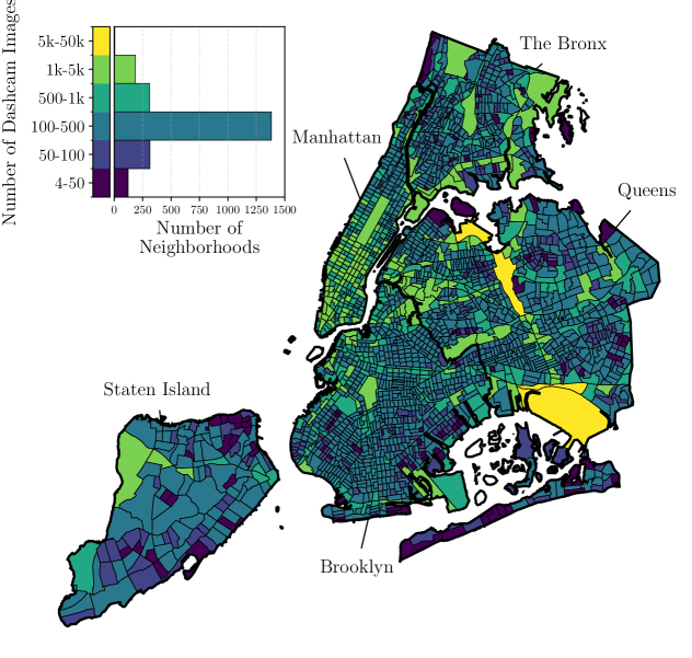
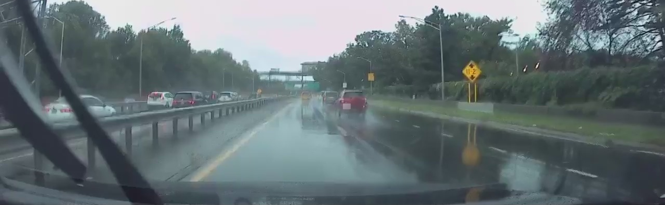
Our dashcam dataset is provided by Nexar, whose data has been widely used in prior work (Dadashova et al., 2021; Franchi et al., 2023, 2024; Shapira et al., 2024; Chowdhury et al., 2024, 2021). Nexar images are 1280 720 pixels and are captured from cameras affixed to the windshield of actively-driving vehicles, mostly those of ridesharing111Ridesharing refers to services that offer on-demand passenger pickup and dropoff at a chosen destination; companies that offer ridesharing include Uber and Lyft. drivers. We develop custom tooling to cull imagery of interest from Nexar’s data moat. Our primary dataset consists of 926,212 images from a storm in New York City on September 29, 2023 which caused widespread flooding. We additionally validate our approach on Nexar images from three other days: 158,555 images from New York City on December 17-18, 2023; 331,034 images from New York City on January 9-10, 2024; and 24,383 images from the San Francisco area (noa, 2025) on February 10, 2024. All dates are chosen because they coincide with storms which caused known flooding events. In our primary analysis dataset on September 9, 2023, the median Census tract contains 220 images, and only 5.2% of tracts have fewer than 50 images.222Census tracts are fine-grained geographic areas within the United States with 4,000 inhabitants on average. New York City has 2,327 Census tracts. Figure 1 depicts the spatial distribution of images, and Figure 2 provides examples of representative images. An important strength of our analysis is that we develop and validate our flood detection method using more than a million spatiotemporally granular dashcam images across flood events from multiple dates and cities. To our knowledge, due to the rarity of floods and the difficulty of collecting temporally dense street scene data at the spatial scale of a city, a dataset with these characteristics has not been previously used.
Ethics
Our use of this dataset has been previously deemed not human subjects research by our institution’s IRB, as our data depicts public street scenes and we do not analyze pedestrians. We are committed to ethical use of our data, and our data provider maintains a high data anonymization standard of blurring pedestrians, license plates, and dashboards prior to us having any access. The data provider additionally blacks out the top and bottom of each image to remove any personally-identifiable information from the driver that may appear on the vehicle dashboard.
 |
 |
3.2. Additional datasets
We make use of the following external datasets relevant to flood risk to contextualize and validate our flood risk predictions.
311 reports
Crowdsourced resident reporting systems like NYC311 have emerged as important indicators of infrastructural problems, including street flooding. In a typical 311 system, residents have the ability to submit reports of non-emergency problems (via app, internet, or phone) which are then routed to the appropriate city agency for remediation (Minkoff, 2016). During the September 29, 2023 storm in New York City, for example, there were 2,171 calls made to 311 pertaining to flooding-related issues (see §A.2 for the list of issues we define as flooding-related). While 311 provides valuable information on potential floods, and is thus a useful external validation of our model’s flood detections, it is also known to contain biases due to disparities in how likely neighborhoods are to report problems (White and Trump, 2018; Kontokosta et al., 2017; Agostini et al., 2024; Kontokosta and Hong, 2021; Clark et al., 2013; O’Brien et al., 2015). We show our approach can be applied to audit these biases.
Physical flooding sensors
Physical flooding sensors are an important current source of flooding signal for cities (Silverman et al., 2022). We rely on data from FloodNet (Mydlarz et al., 2024), a New York City government-academic partnership to develop low-cost, easy-to-assemble flooding sensors and install them throughout high-risk areas. At the time of the flood on which we conduct our primary analysis (September 9, 2023) there were 67 active FloodNet sensors; as of December 12, 2024 (the last update), there are 253 unique FloodNet sensors placed at some point in time. We use the locations of these 253 sensors as an indicator of flood risk. Placement decisions are informed by a detailed, community-informed process (FloodNet NYC, 2025).
Stormwater accumulation maps
Stormwater accumulation maps have been developed as a useful tool for governments and citizens to facilitate flood readiness (Van Alphen et al., 2009; Faber, 2015; Rosenzweig et al., 2024). We use Stormwater Flooding Maps from the New York City Department of Environmental Protection (NYC DEP) (NYC Department of Environmental Protection, [n. d.]), which use simulations that incorporate drainage system data and flow capacity measurements to provide estimates of (1) shallow flooding (more than 4 inches, less than 1 foot) and (2) deep and contiguous flooding (greater than 1 foot). We select a version of the map that simulates a moderate stormwater flood, which best replicates the conditions on the date our primary analysis dataset is collected.
Digital elevation maps (DEM)
We utilize New York City’s Digital Elevation Map (NYC OpenData, 2024) to compute basic elevation metrics for each Census tract in the city, including minimum elevation, mean elevation, and maximum elevation. The DEM was generated with one-foot granularity using LiDAR data, and is meant to ground elevation in feet above sea level, with all built surface features removed.
American Community Survey (ACS) demographic data.
We use the US Census’ American Community Survey to investigate our model’s population coverage and investigate biases in 311 data. Following similar work (Kontokosta and Hong, 2021; Agostini et al., 2024; Kontokosta et al., 2017), we select datasets on total population, reported race and age (U.S. Census Bureau, [n. d.]a), household income (U.S. Census Bureau, [n. d.]c), educational attainment (U.S. Census Bureau, [n. d.]b), access to technology (U.S. Census Bureau, [n. d.]e), and language spoken at home (U.S. Census Bureau, [n. d.]d).
4. Method
We now describe our method, BayFlood. BayFlood has two stages. First, using a VLM, we perform zero-shot classification of whether dashcam images show flooding, and annotate a small number of classified positives and classified negatives with ground-truth human labels (§4.1). Second, we use the classifier labels and the ground-truth annotations as inputs to a Bayesian spatial model which smooths across adjacent areas and incorporates external flood risk features (§4.2). The raw images are not used as inputs to the Bayesian model.
4.1. Zero-shot VLM classification
We perform zero-shot classification of whether each image is flooded using the Cambrian model (NYU VisionX, 2024), an open-source VLM developed in 2024 which achieved state-of-the-art results among open-source models like LLaVA-NeXT (Liu et al., 2024b), and comparable performance to the best proprietary models including GPT-4V (OpenAI et al., 2024) and Gemini-Pro (Team et al., 2024). We use the 13B-parameter version of the model, and use the prompt Does this image show more than a foot of standing water? This prompt was the most performant on the annotated inspection set we describe below, and aligns with the definition of ‘deep’ flooding as defined by the New York City Department of Environmental Protection (NYC Department of Environmental Protection, [n. d.]). We use the 13B-parameter version of Cambrian because it considerably outperforms the smaller 8B-parameter version (Table 1) without introducing the significantly higher inference costs of the 34B-parameter version. Performing inference on all 926,212 images in our primary dataset takes approximately one week when distributed across 6 Nvidia RTX A6000 GPUs. The model classifies 0.2% of images as flooded, consistent with the imbalanced nature of the dataset.
Measuring model performance
We assess Cambrian-1-13B’s performance on our primary dataset by randomly sampling 500 images classified as positive and 500 classified as negative, and manually annotating them. One researcher from the team annotated all images to ensure annotation criteria were consistent. Each image was annotated as positive if it showed definite flooding: namely, the street in front of the vehicle was visible and showed significant flooding. Ambiguous images, and ponding and other small puddles, were marked as negative. We quantify model performance by reporting the positive predictive value (i.e., the proportion of classified positives which are truly positive) and the false omission rate (i.e., the proportion of classified negatives which are truly positive). We also validate model performance on three additional dashcam image datasets from other dates and cities (§3.1).
Comparison to classification baselines
We compare the zero-shot classification performance of Cambrian-1-13B to that of several other VLMs: Cambrian-1-8B, CLIP, and DeepSeek Janus-Pro-7B. We also compare to a supervised learning baseline (a ResNet fine-tuned on a subset of the dataset with flooding labels). We fully describe these baselines in Appendix B. For all models, we compare performance using the same metrics discussed above — namely, for each model, we estimate and by taking a random sample of its positive classifications, and a random sample of its negative classifications, and annotating with ground-truth labels.
4.2. Bayesian modeling of VLM classifications
After classifying all images using the VLM, and manually annotating a small subset of the classified images, we then fit a Bayesian model on the 926,212 model classifications (positive or negative) and manual ground-truth annotations (positive, negative, or unknown). Because we only annotate 1,000 images, the vast majority of annotations are unknown. The raw images are not used as inputs to the Bayesian model.
The purpose of the Bayesian model is to estimate the proportion of images in each Census area which are truly flooded, , while accounting for uncertainty due to classifier error and finite samples of images; smoothing across adjacent areas; and incorporating external data relevant to flood risk.
Observed data
Let denote the manual ground-truth annotation for each image (i.e., whether it truly flooded) and its label from the VLM classifier. In each Census area, we have images of six types, depending on (a) whether the image’s classifier label is positive or negative and (b) the ground-truth annotation label is positive, negative, or unknown (2 possibilities 3 possibilities = 6 image types). Thus, our observed data for each Census area consists of a set of six numbers: the counts of images in the Census area where the classifier label is and the ground-truth label is . For example, the observed data for one Census area with 100 images might be “90 images were classified negative, and have unknown ground-truth label; 9 were classified positive, and have unknown ground-truth label; and 1 was classified positive, and has a positive ground-truth label”. For each Census area we additionally observe a vector of flood-relevant features from the data sources described in §3.2: for example, whether the area is a flood risk zone or has any resident complaints of flooding. (Appendix C.2 lists features and describes feature preprocessing.)
Model
We summarize our model here and provide additional details in Appendix C. Our main quantity of interest is the probability that an image in a Census area shows flooding, . We model this as follows:
where is an intercept term, is the feature coefficients, and is an Intrinsic Conditional Auto-Regressive (ICAR) spatial component which varies by Census area, a standard technique to capture spatially correlated phenomena like flooding (Morris et al., 2019; Besag and Kooperberg, 1995) by smoothing across adjacent areas.
We model VLM classifier errors by introducing parameters to capture the classifier’s true positive rate and false positive rate . We assume these error rates remain constant across Census areas.
The log likelihood (LL) of the observed data in Census area is:
We can write and in terms of and the error rates , allowing us to express the LL of the observed data in terms of the model parameters:
To complete the Bayesian model specification, we place weakly informative priors over all model parameters. We fit the model using Hamiltonian Monte Carlo (HMC) (Neal, 2012; Chen et al., 2014) as implemented in the probabilistic programming language Stan (Carpenter et al., 2017). Below, we will use as shorthand to refer to the model’s inferred flood risk in a given Census tract.
5. Results
We first perform four validations of BayFlood (§5.1), showing that (1) the VLM classifier provides strong signal for detecting flooded images, and outperforms baselines; (2) the Bayesian modeling approach improves out-of-sample prediction relative to baselines; (3) our predictions remain robust even with very few ground-truth annotations; and (4) our inferred measures of flood risk correlate with external ground-truth markers not used in model fitting. Having validated BayFlood, we show that it can be usefully applied to improve flood detection in New York City (§5.2), identifying flooded areas missed by current approaches, revealing inequities in coverage, and suggesting locations for additional flood sensors.
5.1. Method validation
5.1.1. The VLM classifier can detect flooded images
On our primary dataset of images, the VLM classifier displays strong signal for differentiating flooded and non-flooded images. The positive predictive value, , is 0.658, indicating that of the images the VLM classifies as flooded, 65.8% are truly flooded; , indicating that of the images the VLM classifies as not flooded, only 0.6% are truly flooded. Put another way, if the VLM predicts an image is flooded, it is 110 more likely to be flooded. These metrics show both that the classifier clearly provides strong signal for flooding, and that it is imperfect, motivating our use of a Bayesian model to estimate its error rate and incorporate ground-truth annotations. Importantly, Table 1 additionally shows that our chosen model (Cambrian-1-13B) outperforms all classification baselines, achieving higher (, t-test), and lower but comparable (differences not statistically significant, t-test).
| Method | ||
|---|---|---|
| Supervised learning | 0.464 | 0.012 |
| CLIP | 0.224 | 0.008 |
| DeepSeek Janus-Pro-7B | 0.248 | 0.012 |
| Cambrian-1-8B | 0.152 | 0.012 |
| Cambrian-1-13B (ours) | 0.658 | 0.006 |
We assess how well the VLM classifier generalizes to other days and cities by measuring its performance during two other floods in New York City and an additional flood in the San Francisco Bay area (§3.1). Performance remains strong (Table S2): images which are classified as flooded are at least333In our three validation datasets, we do not observe any false negatives among the images classified negative. We thus compute these numbers using an upper bound of one false negative. 351, 406, and 72 times likelier to be flooded than images which are not across the three days.
5.1.2. Bayesian modeling improves out-of-sample prediction
Having validated the first stage of BayFlood (VLM classification of whether flooding occurs) we now validate the second (fitting a spatial Bayesian model on the classifications). Specifically, we show that our Bayesian approach improves predictions of where flooded images will occur on a held-out test set, relative to both simple heuristics (e.g., the fraction of images which are classified as positive by the VLM) and machine learning baselines.
We perform this validation as follows. After classifying the 926,212 images in our primary dataset with the VLM, we partition them into a train set (which we use to fit the Bayesian model and the baselines on the classifications) and a test set (which we use to assess out-of-sample performance). We use three metrics to assess predictive performance on the Census tract level: (1) Pearson correlation with fraction of images in the tract which are classified flooded; (2) AUC for predicting whether the Census tract will have any classified flooded images; (3) AUC for predicting whether the Census tract will have any ground-truth annotated flooded images. To minimize the noisiness of these metrics on the test set, we reserve 70% of the dataset for the test set. Thus, the train set for this validation consists of the VLM classifications , and ground-truth annotations , for 30% of the images; the test set consists of the VLM classifications and ground-truth annotations for the remaining 70%.
We compare to three sets of baselines. First, we compare to several heuristic baselines (i.e., simple functions of the VLM classifications or ground-truth annotations which do not require machine learning): (1) the fraction of train set images in a Census tract which are classified positive by the VLM; (2) the number of train set images which are classified positive; (3) whether any train set images are classified positive; (4) whether any train set images are ground-truth annotated positive; and (5) the number of train set images which are ground-truth annotated positive. Second, we compare to supervised learning baselines which are trained on the train set to predict the fraction of images which are classified as flooded, and the number of ground-truth annotated flooded images, from the same set of flood-relevant features our Bayesian model uses (Appendix C). We fit both linear regression and random forest models. Finally, we compare a graph smoothing baseline, which applies Laplacian smoothing using the Census tract adjacency matrix. We fully describe all baselines in Appendix C.3.
Our Bayesian model outperforms all baselines on all considered metrics (Table 2), demonstrating it provides benefit over alternative ways of aggregating the VLM annotations.
| Method |
Pearson [frac +
classifications] |
AUC
[any ground-truth +] |
AUC
[any + classifications] |
|---|---|---|---|
| Frac. + classifications | |||
| Any + classfications? | |||
| # + classifications | |||
| Any + annotations? | |||
| # + annotations | |||
| OLS | |||
| Random Forest | |||
| Laplacian smoothing | |||
| BayFlood | 0.57 0.04 | 0.88 0.01 | 0.79 0.01 |
5.1.3. Model predictions remain stable even with very few ground-truth annotations
Because ground-truth human annotations can be expensive to produce in some settings, we investigate whether the flood risk predictions of our Bayesian model, , remain stable even with very few ground-truth annotations, showing that the model can be reliably applied even when annotations are sparse. Specifically, we refit the Bayesian model on datasets where the number of ground-truth annotations have been downsampled by a factor of 2 - 20; 20 downsampling corresponds to only 25 annotated positives and 25 annotated negatives. We find that the model’s predictions on these downsampled datasets remain highly correlated with predictions on the full dataset (between 0.89 - 0.94 across all downsampling ratios). This suggests that our Bayesian approach can be applied even in settings where very few ground-truth annotations can be collected. Further, because the Bayesian model yields measures of uncertainty on all estimates, it naturally provides principled estimates of the stability of model predictions, guiding the collection of additional annotations if needed.
no 311 reports.
no sensors.
no stormwater predictions.
5.1.4. Inferred flood risk correlates with known markers of flood risk
We assess whether our Census-tract-specific estimates of flood risk correlate with the external markers of flood risk discussed in §3.2 (Figure S4). For this analysis, we fit our Bayesian model without incorporating any of these external features, so we are assessing the model’s consistency with external flood risk markers it does not have access to. We define a census tract as “high BayFlood risk” if either , where is the set of all tracts with a confirmed ground-truth annotated flood image, or if , where is the 25th percentile of among all tracts in . We find that BayFlood’s predictions indeed predict external markers of flood risk: its high-risk Census tracts are 1.4 likelier to have a 311 report and 2.0 likelier to have a FloodNet sensor. Their minimum elevation is 2.0 lower and they have 1.3 larger shallow stormwater accumulation zones as assessed by the Department of Environmental Protection and 1.2 more deep stormwater accumulation zones. (All differences are statistically significant except deep stormwater accumulation zones (p=0.068); , t-test).
5.2. Improving flood detection in New York City
Having validated BayFlood, we show it can be applied to three important use cases: detecting flooded areas missed by existing methods; quantifying biases in 311 reports; and suggesting new locations for flood sensors. These applications are informed by our conversations with government decision-makers as well as with academic-government partnerships like FloodNet.
5.2.1. Detecting flooded areas missed by existing methods
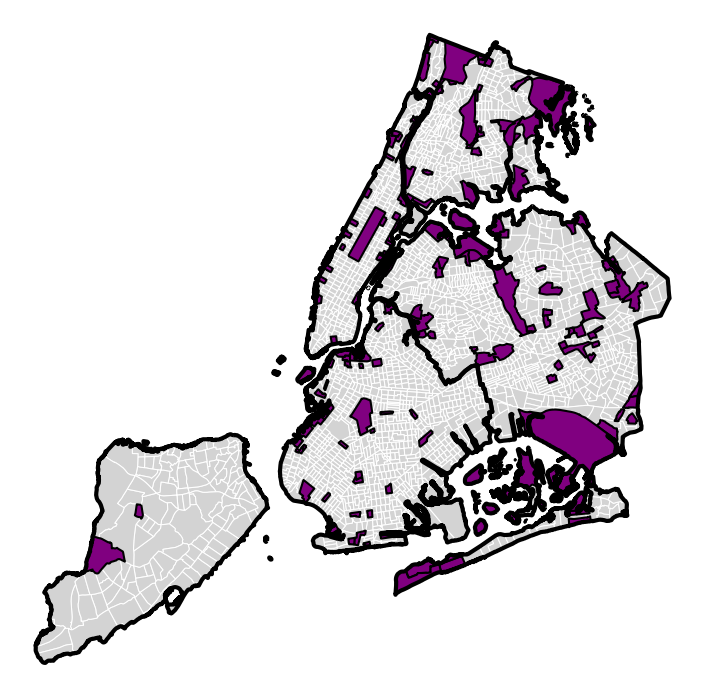
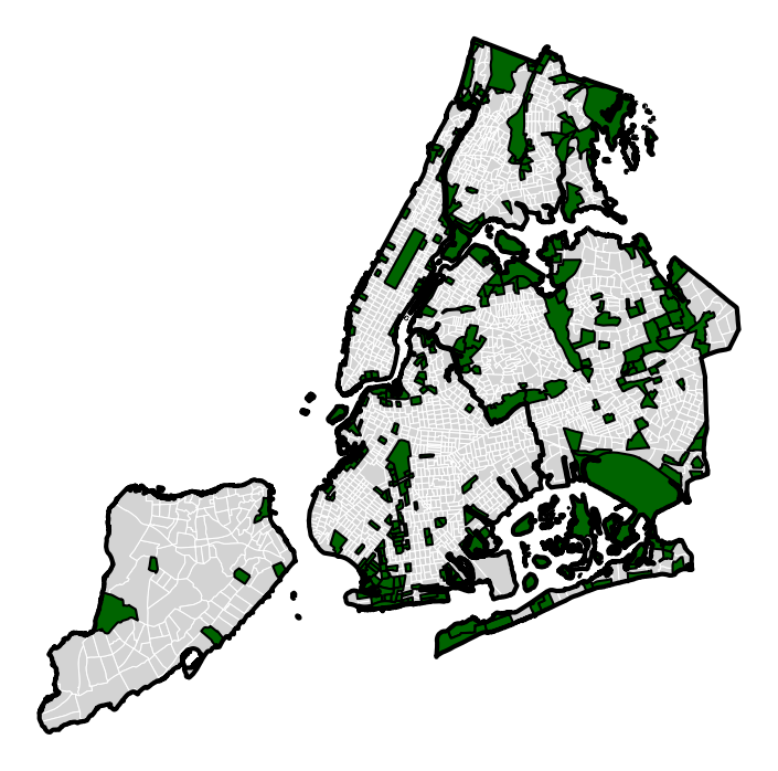
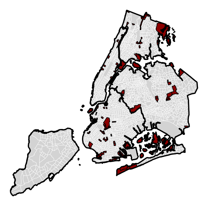
Our model can identify Census tracts at risk for flooding which are missed by methods currently used by urban decision-makers (Figure 3). We quantify the number of Census tracts that are predicted high-risk by BayFlood but do not have a flood-related 311 report, a FloodNet sensor, or predicted stormwater accumulation. (For this analysis, we define tracts with high BayFlood risk as in §5.1.4.)
1,003,940 people live in the Census tracts with high BayFlood risk, comprising 12% of New York City’s population. Of these, 433,079 people live in Census tracts with no flooding-related 311 reports; 927,908 people live in Census tracts with no FloodNet sensors; 293,095 people live in Census tracts with no predicted stormwater accumulation; and 113,738 people live in Census tracts with no indicator of flood risk from any of these methods.444Supplementary Figure S3 reports a version of this analysis redefining “high flood risk” tracts as those at least one ground-truth confirmed flooded image (); this similarly identifies many tracts which are missed by current flood detection methods, though not as many as those identified by our Bayesian model, highlighting the benefits of our approach. Collectively, these results indicate that our model can identify large populations of people who face flood risks currently overlooked by some or all of the existing flood detection methods.
5.2.2. Quantifying biases in 311 reports
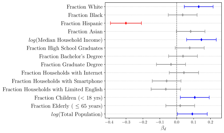
Previous work has raised concerns that 311 reports may display demographic biases, with some neighborhoods less likely to report incidents when they occur (Agostini et al., 2024; Kontokosta and Hong, 2021; Kontokosta et al., 2017). We investigate whether our model can quantify these biases. Specifically, we conduct a risk-adjusted logistic regression (Jung et al., 2018), which assesses whether there are demographic disparities in 311 reporting patterns across Census tracts which cannot be explained by our model’s estimated flood risk:
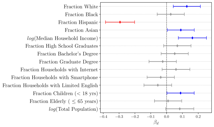
where is an intercept term; is our model’s estimate of flood risk in tract ; is a demographic feature555All demographic data comes from the American Community Survey 2023 5-Year Estimates. (e.g., the fraction of the tract which is white); and the s are the regression coefficients. Figure 4 plots the estimated demographic coefficients . Controlling for flood risk, we find that Census tracts with larger fractions of white and Asian residents, lower fractions of Hispanic residents, higher average household incomes, and higher fractions of children are statistically significantly likelier to have a 311 report. These findings accord with past work providing evidence of biases in 311 reporting patterns, and show that our model can be usefully applied to audit existing methods of flood detection.666Supplementary Figure S5 repeats this analysis controlling for an alternate measure of flood risk: whether a tract has at least one ground-truth confirmed flooded image (); results are similar.
5.2.3. Suggesting new locations for sensor placement
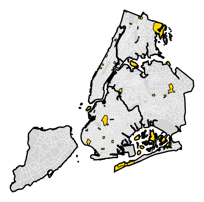
Based on our finding that many Census tracts have no flood sensors, but high predicted flood risk, we provide a proof-of-concept illustration that our model can be applied to identify tracts which might benefit from the placement of a new sensor.
We assume that if a sensor is placed in a given tract, it can detect a flood in all tracts within a -hop neighborhood, because floods are spatially correlated. We set in our experiments, but our framework can easily be applied to other (as well as to incorporate additional considerations like the population of a tract, equity in sensor placement, etc). Given the current locations of sensors in a set of Census tracts , our task is to place an additional sensors in a set of Census tracts to maximize the sum of flood risk in covered areas:
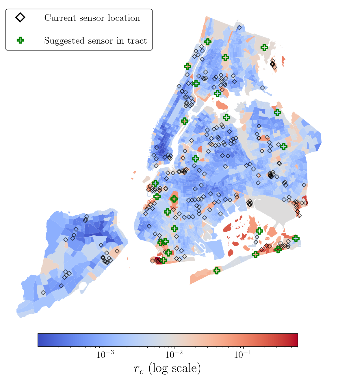
where denotes all Census tracts in the neighborhood of set . This is a weighted maximum coverage problem (Nemhauser et al., 1978) in which we are given a collection of sets, and our goal is to choose sets such that the weighted sum of elements is maximized. Here, each set is the tracts covered by a sensor in a given location, and the weight for each tract is . This problem is NP-hard, but because the optimization objective is submodular, the greedy solution achieves an approximation ratio of , and is often used. At each iteration, we greedily choose the Census tract that maximizes the sum of in newly covered tracts. We plot the locations chosen by this procedure in Figure 5, setting . We are submitting our suggested locations to the FloodNet collaboration (Mydlarz et al., 2024) as part of our ongoing conversations with them regarding sensor placements. They expressed interest in our data and methodology as one valuable source of signal to supplement their ongoing placement methodology, which is largely driven by community engagement, stakeholder needs, and equity considerations (Ceferino et al., 2023).
6. Discussion
In this work, we developed a novel two-stage method, BayFlood, that combines modern VLMs with classical Bayesian spatial modeling to detect urban incidents such as street flooding. In the first stage, we conduct zero-shot classification using a pre-trained VLM to identify flooding in street images, avoiding the need for large labeled datasets. In the second stage, the results from this classification are integrated into a Bayesian spatial model; this provides the benefits of classical statistical methods, including principled measures of uncertainty, spatial smoothing, and incorporation of external datasets. We show that our approach can effectively detect floods and improves on baseline approaches. We apply our methodology to detect floods missed by existing urban detection methods; reveal biases in current approaches; and suggest locations for new flood sensors.
There are several natural directions for future work. Within urban data science, one might expand our approach to additional cities and flood events. Creating a model which could run in real time, providing insight into ongoing floods, might also offer significant benefits to decision-makers. One might also expand our approach to detect other types of urban incidents, like unpermitted sidewalk scaffolding (Shapira et al., 2024), double parking, or out-of-place garbage; a significant benefit of our methodology is that it relies only on zero-shot detection, avoiding the need for large labeled datasets and easing its application to new types of incidents. Methodologically, there are also avenues for future work, including experimenting with alternate VLMs or model prompts and using temporal or hierarchical Bayesian models which allow for change over time and incorporation of additional storms. More broadly, our results showcase how Bayesian modeling of zero-shot foundation model annotations represents a promising paradigm which combines the power of foundation models with the benefits of classical statistical methods. This paradigm has broad potential applicability in the many settings in the natural and social sciences where foundation models are increasingly being used for annotation.
Code release.
All code and aggregated data for replicating our analysis (including our VLM inferences) are available at this GitHub repository.
Acknowledgements.
We thank Gabriel Agostini, Sidhika Balachandar, Serina Chang, Zhi Liu, and Anna McClendon for useful discussion and feedback. We thank Nexar for data access under research evaluation and project support. We thank Anthony Townsend and Michael Samuelian for project support. We thank the NYC Department of Environmental Protection for helpful discussions. We thank the FloodNet team for helpful discussions and access to FloodNet data. We thank the Digital Life Initiative, the Urban Tech Hub at Cornell Tech, a Google Research Scholar award, an AI2050 Early Career Fellowship, NSF CAREER #2142419, NSF CAREER IIS-2339427, a CIFAR Azrieli Global scholarship, a gift to the LinkedIn-Cornell Bowers CIS Strategic Partnership, the Survival and Flourishing Fund, and the Abby Joseph Cohen Faculty Fund for funding.References
- (1)
- noa (2025) 2025. February 2024 California atmospheric rivers. https://en.wikipedia.org/w/index.php?title=February_2024_California_atmospheric_rivers&oldid=1271259675 Page Version ID: 1271259675.
- Agonafir et al. (2022a) Candace Agonafir, Tarendra Lakhankar, Reza Khanbilvardi, Nir Krakauer, Dave Radell, et al. 2022a. A machine learning approach to evaluate the spatial variability of New York City’s 311 street flooding complaints. Computers, Environment and Urban Systems 97 (Oct. 2022), 101854. https://doi.org/10.1016/j.compenvurbsys.2022.101854
- Agonafir et al. (2022b) Candace Agonafir, Alejandra Ramirez Pabon, Tarendra Lakhankar, Reza Khanbilvardi, and Naresh Devineni. 2022b. Understanding New York City street flooding through 311 complaints. Journal of Hydrology 605 (Feb. 2022), 127300. https://doi.org/10.1016/j.jhydrol.2021.127300
- Agostini et al. (2024) Gabriel Agostini, Emma Pierson, and Nikhil Garg. 2024. A Bayesian Spatial Model to Correct Under-Reporting in Urban Crowdsourcing. Proceedings of the AAAI Conference on Artificial Intelligence 38, 20 (March 2024), 21888–21896. https://doi.org/10.1609/aaai.v38i20.30190 Number: 20.
- Alizadeh et al. (2022) Bahareh Alizadeh, Diya Li, Julia Hillin, Michelle A. Meyer, Courtney M. Thompson, et al. 2022. Human-centered flood mapping and intelligent routing through augmenting flood gauge data with crowdsourced street photos. Advanced Engineering Informatics 54 (Oct. 2022), 101730. https://doi.org/10.1016/j.aei.2022.101730
- Angelopoulos et al. (2023) Anastasios N Angelopoulos, Stephen Bates, Clara Fannjiang, Michael I Jordan, and Tijana Zrnic. 2023. Prediction-powered inference. Science 382, 6671 (2023), 669–674.
- AON (2023) AON. 2023. Weekly Catastrophe Report. Technical Report. AON. https://img.clients.aonunited.com/Web/Aon5/%7B73f84cb4-5186-4b84-81a1-8655b119b981%7D_20231006-1-cat-alert.pdf
- Arthur et al. (2018) Rudy Arthur, Chris A. Boulton, Humphrey Shotton, and Hywel T. P. Williams. 2018. Social sensing of floods in the UK. PLOS ONE (2018). https://doi.org/10.1371/journal.pone.0189327
- Balachandar et al. (2023) Sidhika Balachandar, Nikhil Garg, and Emma Pierson. 2023. Domain constraints improve risk prediction when outcome data is missing. arXiv preprint arXiv:2312.03878 (2023).
- Balachandar et al. ([n. d.]) Sidhika Balachandar, Shuvom Sadhuka, Bonnie Berger, Emma Pierson, and Nikhil Garg. [n. d.]. Using GNNs to Model Biased Crowdsourced Data for Urban Applications. ([n. d.]).
- Berland and Lange (2017) Adam Berland and Daniel A. Lange. 2017. Google Street View shows promise for virtual street tree surveys. Urban Forestry & Urban Greening 21 (Jan. 2017), 11–15. https://doi.org/10.1016/j.ufug.2016.11.006
- Besag and Kooperberg (1995) Julian Besag and Charles Kooperberg. 1995. On conditional and intrinsic autoregressions. Biometrika 82, 4 (1995), 733–746.
- Bhola et al. (2018) Punit Kumar Bhola, Bhavana B. Nair, Jorge Leandro, Sethuraman N. Rao, and Markus Disse. 2018. Flood inundation forecasts using validation data generated with the assistance of computer vision. Journal of Hydroinformatics 21, 2 (Dec. 2018), 240–256. https://doi.org/10.2166/hydro.2018.044
- Biljecki and Ito (2021) Filip Biljecki and Koichi Ito. 2021. Street view imagery in urban analytics and GIS: A review. Landscape and Urban Planning 215 (Nov. 2021), 104217. https://doi.org/10.1016/j.landurbplan.2021.104217
- Brakenridge et al. (2003) G R Brakenridge, S V Nghiemb, and B Shabaneh. 2003. Flood Warnings, Flood Disaster Assessments, and Flood Hazard Reduction: The Roles of Orbital Remote Sensing. (2003).
- Branson et al. (2018) Steve Branson, Jan Dirk Wegner, David Hall, Nico Lang, Konrad Schindler, et al. 2018. From Google Maps to a fine-grained catalog of street trees. ISPRS Journal of Photogrammetry and Remote Sensing 135 (Jan. 2018), 13–30. https://doi.org/10.1016/j.isprsjprs.2017.11.008
- Brody et al. (2007) Samuel D. Brody, Sammy Zahran, Praveen Maghelal, Himanshu Grover, and Wesley E. Highfield. 2007. The Rising Costs of Floods: Examining the Impact of Planning and Development Decisions on Property Damage in Florida. Journal of the American Planning Association 73, 3 (Sept. 2007), 330–345. https://doi.org/10.1080/01944360708977981 Publisher: Routledge _eprint: https://doi.org/10.1080/01944360708977981.
- Campbell et al. (2019) Andrew Campbell, Alan Both, and Qian (Chayn) Sun. 2019. Detecting and mapping traffic signs from Google Street View images using deep learning and GIS. Computers, Environment and Urban Systems 77 (Sept. 2019), 101350. https://doi.org/10.1016/j.compenvurbsys.2019.101350
- Carpenter et al. (2017) Bob Carpenter, Andrew Gelman, Matthew D Hoffman, Daniel Lee, Ben Goodrich, et al. 2017. Stan: A probabilistic programming language. Journal of statistical software 76 (2017).
- Ceferino et al. (2023) Luis Ceferino, Andrea Silverman, Elizabeth Henaff, Charlie Mydlarz, Tega Brain, et al. 2023. Developing a Framework to Optimize Floodnet Sensor Deployments around NYC for Equitable and Impact-Based Hyper-Local Street-Level Flood Monitoring and Data Collection. Technical Report. https://rosap.ntl.bts.gov/view/dot/68526
- Chaudhary et al. (2019) Priyanka Chaudhary, M. Moy de Vitry, João P. Leitão, and Jan Dirk Wegner. 2019. Flood-Water Level Estimation from Social Media Images. ISPRS Annals of the Photogrammetry, Remote Sensing and Spatial Information Sciences (2019). https://doi.org/10.5194/isprs-annals-iv-2-w5-5-2019
- Chen et al. (2014) Tianqi Chen, Emily Fox, and Carlos Guestrin. 2014. Stochastic gradient hamiltonian monte carlo. In International conference on machine learning. PMLR, 1683–1691.
- Chen et al. (2025) Xiaokang Chen, Zhiyu Wu, Xingchao Liu, Zizheng Pan, Wen Liu, et al. 2025. Janus-Pro: Unified Multimodal Understanding and Generation with Data and Model Scaling. https://doi.org/10.48550/arXiv.2501.17811 arXiv:2501.17811 [cs].
- Chen et al. (2019) Yu Chen, Lingfei Wu, and Mohammed J. Zaki. 2019. Deep Iterative and Adaptive Learning for Graph Neural Networks. https://doi.org/10.48550/arXiv.1912.07832 arXiv:1912.07832 [cs].
- Cherian et al. (2024) John J Cherian, Isaac Gibbs, and Emmanuel J Candès. 2024. Large language model validity via enhanced conformal prediction methods. arXiv preprint arXiv:2406.09714 (2024).
- Chiang et al. (2024) Erica Chiang, Divya Shanmugam, Ashley N Beecy, Gabriel Sayer, Nir Uriel, et al. 2024. Learning Disease Progression Models That Capture Health Disparities. arXiv preprint arXiv:2412.16406 (2024).
- Chowdhury et al. (2021) Tahiya Chowdhury, Ansh Bhatti, Ilan Mandel, Taqiya Ehsan, Wendy Ju, et al. 2021. Towards sensing urban-scale COVID-19 policy compliance in new york city. In Proceedings of the 8th ACM International Conference on Systems for Energy-Efficient Buildings, Cities, and Transportation. ACM, Coimbra Portugal, 353–356. https://doi.org/10.1145/3486611.3491123
- Chowdhury et al. (2024) Tahiya Chowdhury, Ilan Mandel, Jorge Ortiz, and Wendy Ju. 2024. Designing a User-centric Framework for Information Quality Ranking of Large-scale Street View Images. https://doi.org/10.48550/arXiv.2404.00392 arXiv:2404.00392 [cs].
- Clark et al. (2013) Benjamin Y Clark, Jeffrey L Brudney, and Sung-Gheel Jang. 2013. Coproduction of government services and the new information technology: Investigating the distributional biases. Public Administration Review 73, 5 (2013), 687–701.
- Dadashova et al. (2021) Bahar Dadashova, Chiara Silvestri Dobrovolny, and Mahmood Tabesh. 2021. Detecting pavement distresses using crowdsourced dashcam camera images. Technical Report. Safety through Disruption (Safe-D) University Transportation Center (UTC). https://rosap.ntl.bts.gov/view/dot/60311
- Desmet et al. (2018) Klaus Desmet, Robert E. Kopp, Scott A. Kulp, Dávid Krisztián Nagy, Michael Oppenheimer, et al. 2018. Evaluating the Economic Cost of Coastal Flooding. https://doi.org/10.3386/w24918
- Devitt et al. (2023) Laura Devitt, Jeffrey Neal, Gemma Coxon, James Savage, and Thorsten Wagener. 2023. Flood hazard potential reveals global floodplain settlement patterns. Nature Communications 14 (May 2023), 2801. https://doi.org/10.1038/s41467-023-38297-9
- Faber (2015) Jacob William Faber. 2015. Superstorm Sandy and the demographics of flood risk in New York City. Human Ecology 43 (2015), 363–378. https://idp.springer.com/authorize/casa?redirect_uri=https://link.springer.com/article/10.1007/s10745-015-9757-x&casa_token=3x95XNBv-zQAAAAA:q8ZY1gqMgpbPgI9j8FRAhvRFUYs2HpfYN4CyNdSRZ_znF53M2UdjPFqLlkKzCImw9DOBa7lJxUh3Oe2c Publisher: Springer.
- FloodNet NYC (2025) FloodNet NYC. 2025. Community Engagement. https://www.floodnet.nyc/home-1-1
- Franchi et al. (2024) Matt Franchi, Debargha Dey, and Wendy Ju. 2024. Towards Instrumented Fingerprinting of Urban Traffic: A Novel Methodology using Distributed Mobile Point-of-View Cameras. In Proceedings of the 16th International Conference on Automotive User Interfaces and Interactive Vehicular Applications (AutomotiveUI ’24). Association for Computing Machinery, New York, NY, USA, 53–62. https://doi.org/10.1145/3640792.3675740
- Franchi et al. (2023) Matt Franchi, J.D. Zamfirescu-Pereira, Wendy Ju, and Emma Pierson. 2023. Detecting disparities in police deployments using dashcam data. In Proceedings of the 2023 ACM Conference on Fairness, Accountability, and Transparency (FAccT ’23). Association for Computing Machinery, New York, NY, USA, 534–544. https://doi.org/10.1145/3593013.3594020
- Franchi, Matt et al. (2025) Franchi, Matt, Parreira, Maria Teresa, Bu, Frank, and Ju, Wendy. 2025. The Robotability Score: Enabling Harmonius Robot Navigation on Urban Streets. In Proceedings of the 2025 SIGCHI Conference on Human Factors in Computing Systems. ACM. https://doi.org/10.1145/3706598.3714009
- Friedman (2009) Jerome Friedman. 2009. The elements of statistical learning: Data mining, inference, and prediction. (No Title) (2009). https://cir.nii.ac.jp/crid/1370846644385113871
- Gebru et al. (2017) Timnit Gebru, Jonathan Krause, Yilun Wang, Duyun Chen, Jia Deng, et al. 2017. Using deep learning and Google Street View to estimate the demographic makeup of neighborhoods across the United States. Proceedings of the National Academy of Sciences 114, 50 (Dec. 2017), 13108–13113. https://doi.org/10.1073/pnas.1700035114 Publisher: Proceedings of the National Academy of Sciences.
- Geetha et al. (2017) M. Kalaiselvi Geetha, Megha Manoj, A. S. Sarika, Muktha Mohan, and Sethuraman N. Rao. 2017. Detection and estimation of the extent of flood from crowd sourced images. null (2017). https://doi.org/10.1109/iccsp.2017.8286429
- Gelman et al. (1995) Andrew Gelman, John B Carlin, Hal S Stern, and Donald B Rubin. 1995. Bayesian data analysis. Chapman and Hall/CRC.
- Gligorić et al. (2024) Kristina Gligorić, Tijana Zrnic, Cinoo Lee, Emmanuel J Candès, and Dan Jurafsky. 2024. Can Unconfident LLM Annotations Be Used for Confident Conclusions? arXiv preprint arXiv:2408.15204 (2024).
- Haas et al. (2023) Lukas Haas, Silas Alberti, and Michal Skreta. 2023. Learning Generalized Zero-Shot Learners for Open-Domain Image Geolocalization. https://doi.org/10.48550/arXiv.2302.00275 arXiv:2302.00275 [cs].
- Hao et al. (2022) Xin Hao, Heng Lyu, Ze Wang, Shengnan Fu, and Chi Zhang. 2022. Estimating the spatial-temporal distribution of urban street ponding levels from surveillance videos based on computer vision. Water Resources Management 36, 6 (April 2022), 1799–1812. https://doi.org/10.1007/s11269-022-03107-2
- Hara et al. (2014) Kotaro Hara, Jin Sun, Robert Moore, David Jacobs, and Jon Froehlich. 2014. Tohme: detecting curb ramps in google street view using crowdsourcing, computer vision, and machine learning. In Proceedings of the 27th annual ACM symposium on User interface software and technology (UIST ’14). Association for Computing Machinery, New York, NY, USA, 189–204. https://doi.org/10.1145/2642918.2647403
- Hinkel et al. (2014) Jochen Hinkel, Daniel Lincke, Athanasios T. Vafeidis, Mahé Perrette, Robert James Nicholls, et al. 2014. Coastal flood damage and adaptation costs under 21st century sea-level rise. Proceedings of the National Academy of Sciences 111, 9 (March 2014), 3292–3297. https://doi.org/10.1073/pnas.1222469111 Publisher: Proceedings of the National Academy of Sciences.
- Huang et al. (2024) Weiming Huang, Jing Wang, and Gao Cong. 2024. Zero-shot urban function inference with street view images through prompting a pretrained vision-language model. International Journal of Geographical Information Science 38, 7 (July 2024), 1414–1442. https://doi.org/10.1080/13658816.2024.2347322 Publisher: Taylor & Francis _eprint: https://doi.org/10.1080/13658816.2024.2347322.
- Ilic et al. (2019) Lazar Ilic, M. Sawada, and Amaury Zarzelli. 2019. Deep mapping gentrification in a large Canadian city using deep learning and Google Street View. PLOS ONE 14, 3 (March 2019), e0212814. https://doi.org/10.1371/journal.pone.0212814 Publisher: Public Library of Science.
- Jafari et al. (2021) Navid H. Jafari, Xin Li, Qin Chen, Can-Yu Le, Logan P. Betzer, et al. 2021. Real-time water level monitoring using live cameras and computer vision techniques. Computers & Geosciences 147 (Feb. 2021), 104642. https://doi.org/10.1016/j.cageo.2020.104642
- Janssen et al. (2012) Marijn Janssen, Yannis Charalabidis, and Anneke Zuiderwijk. 2012. Benefits, Adoption Barriers and Myths of Open Data and Open Government. Information Systems Management 29, 4 (Sept. 2012), 258–268. https://doi.org/10.1080/10580530.2012.716740
- Jung et al. (2018) Jongbin Jung, Sam Corbett-Davies, Johann D Gaebler, Ravi Shroff, and Sharad Goel. 2018. Mitigating included-and omitted-variable bias in estimates of disparate impact. arXiv preprint arXiv:1809.05651 (2018).
- Kim and Jang (2023) Junghwan Kim and Kee Moon Jang. 2023. An examination of the spatial coverage and temporal variability of Google Street View (GSV) images in small- and medium-sized cities: A people-based approach. Computers, Environment and Urban Systems 102 (June 2023), 101956. https://doi.org/10.1016/j.compenvurbsys.2023.101956
- Klemas (2014) Victor Klemas. 2014. Remote Sensing of Floods and Flood-Prone Areas: An Overview. Journal of Coastal Research 31, 4 (Dec. 2014), 1005–1013. https://doi.org/10.2112/JCOASTRES-D-14-00160.1
- Kontokosta et al. (2017) Constantine Kontokosta, Boyeong Hong, and Kristi Korsberg. 2017. Equity in 311 Reporting: Understanding Socio-Spatial Differentials in the Propensity to Complain. https://doi.org/10.48550/arXiv.1710.02452 arXiv:1710.02452 [cs].
- Kontokosta and Hong (2021) Constantine E. Kontokosta and Boyeong Hong. 2021. Bias in smart city governance: How socio-spatial disparities in 311 complaint behavior impact the fairness of data-driven decisions. Sustainable Cities and Society 64 (Jan. 2021), 102503. https://doi.org/10.1016/j.scs.2020.102503
- Laufer et al. (2022) Benjamin Laufer, Emma Pierson, and Nikhil Garg. 2022. End-to-end Auditing for Decision Pipelines.. In ICML Workshop on Responsible Decision Making in Dynamic Environments (RDMDE).
- Li et al. (2018a) Qimai Li, Zhichao Han, and Xiao-Ming Wu. 2018a. Deeper insights into graph convolutional networks for semi-supervised learning. In Proceedings of the AAAI conference on artificial intelligence, Vol. 32. https://ojs.aaai.org/index.php/AAAI/article/view/11604 Issue: 1.
- Li et al. (2018b) Xiaojiang Li, Carlo Ratti, and Ian Seiferling. 2018b. Quantifying the shade provision of street trees in urban landscape: A case study in Boston, USA, using Google Street View. Landscape and Urban Planning 169 (Jan. 2018), 81–91. https://doi.org/10.1016/j.landurbplan.2017.08.011
- Liang et al. (2023) Yongqing Liang, Xin Li, Brian Tsai, Qin Chen, and Navid Jafari. 2023. V-FloodNet: A video segmentation system for urban flood detection and quantification. Environmental Modelling & Software 160 (Feb. 2023), 105586. https://doi.org/10.1016/j.envsoft.2022.105586
- Liu et al. (2024b) Haotian Liu, Chunyuan Li, Yuheng Li, Bo Li, Yuanhan Zhang, et al. 2024b. Llava-next: Improved reasoning, ocr, and world knowledge. https://hliu.cc/publications/
- Liu et al. (2024a) Zhi Liu, Uma Bhandaram, and Nikhil Garg. 2024a. Quantifying spatial under-reporting disparities in resident crowdsourcing. Nature Computational Science 4, 1 (2024), 57–65.
- Liu and Garg (2024) Zhi Liu and Nikhil Garg. 2024. Redesigning service level agreements: Equity and efficiency in city government operations. arXiv preprint arXiv:2410.14825 (2024).
- Liu et al. (2024c) Zhi Liu, Sarah Rankin, and Nikhil Garg. 2024c. Identifying and addressing disparities in public libraries with Bayesian latent variable modeling. In Proceedings of the AAAI Conference on Artificial Intelligence, Vol. 38. 22258–22265. https://ojs.aaai.org/index.php/AAAI/article/view/30231 Issue: 20.
- Mason et al. (2012) David C. Mason, Ian J. Davenport, Jeffrey C. Neal, Guy J.-P. Schumann, and Paul D. Bates. 2012. Near Real-Time Flood Detection in Urban and Rural Areas Using High-Resolution Synthetic Aperture Radar Images. IEEE Transactions on Geoscience and Remote Sensing 50, 8 (Aug. 2012), 3041–3052. https://doi.org/10.1109/TGRS.2011.2178030 Conference Name: IEEE Transactions on Geoscience and Remote Sensing.
- Mauerman et al. (2022) Max Mauerman, Elizabeth Tellman, Upmanu Lall, Marco Tedesco, Paolo Colosio, et al. 2022. High-Quality Historical Flood Data Reconstruction in Bangladesh Using Hidden Markov Models. In Water Management: A View from Multidisciplinary Perspectives, G. M. Tarekul Islam, Shampa Shampa, and Ahmed Ishtiaque Amin Chowdhury (Eds.). Springer International Publishing, Cham, 191–210. https://doi.org/10.1007/978-3-030-95722-3_10
- McLafferty et al. (2020) Sara McLafferty, Daniel Schneider, and Kathryn Abelt. 2020. Placing volunteered geographic health information: Socio-spatial bias in 311 bed bug report data for New York City. Health & Place 62 (March 2020), 102282. https://doi.org/10.1016/j.healthplace.2019.102282
- Minkoff (2016) Scott L. Minkoff. 2016. NYC 311: A Tract-Level Analysis of Citizen–Government Contacting in New York City. Urban Affairs Review 52, 2 (March 2016), 211–246. https://doi.org/10.1177/1078087415577796 Publisher: SAGE Publications Inc.
- Mohri and Hashimoto (2024) Christopher Mohri and Tatsunori Hashimoto. 2024. Language models with conformal factuality guarantees. arXiv preprint arXiv:2402.10978 (2024).
- Morris et al. (2019) Mitzi Morris, Katherine Wheeler-Martin, Dan Simpson, Stephen J Mooney, Andrew Gelman, et al. 2019. Bayesian hierarchical spatial models: Implementing the Besag York Mollié model in stan. Spatial and spatio-temporal epidemiology 31 (2019), 100301.
- Mosavi et al. (2018) Amir Mosavi, Pinar Ozturk, and Kwok-wing Chau. 2018. Flood Prediction Using Machine Learning Models: Literature Review. Water 10, 11 (Nov. 2018), 1536. https://doi.org/10.3390/w10111536 Number: 11 Publisher: Multidisciplinary Digital Publishing Institute.
- Mousa et al. (2016) Mustafa Mousa, Xiangliang Zhang, and Christian Claudel. 2016. Flash Flood Detection in Urban Cities Using Ultrasonic and Infrared Sensors. IEEE Sensors Journal 16, 19 (Oct. 2016), 7204–7216. https://doi.org/10.1109/JSEN.2016.2592359 Conference Name: IEEE Sensors Journal.
- Munawar et al. (2022) Hafiz Suliman Munawar, Ahmed W. A. Hammad, and S. Travis Waller. 2022. Remote Sensing Methods for Flood Prediction: A Review. Sensors 22, 3 (Jan. 2022), 960. https://doi.org/10.3390/s22030960 Number: 3 Publisher: Multidisciplinary Digital Publishing Institute.
- Mydlarz et al. (2024) Charlie Mydlarz, Praneeth Sai Venkat Challagonda, Bea Steers, Jeremy Rucker, Tega Brain, et al. 2024. FloodNet: Low-Cost Ultrasonic Sensors for Real-Time Measurement of Hyperlocal, Street-Level Floods in New York City. Water Resources Research 60, 5 (2024), e2023WR036806. https://doi.org/10.1029/2023WR036806 _eprint: https://onlinelibrary.wiley.com/doi/pdf/10.1029/2023WR036806.
- Naik et al. (2017) Nikhil Naik, Scott Duke Kominers, Ramesh Raskar, Edward L. Glaeser, and César A. Hidalgo. 2017. Computer vision uncovers predictors of physical urban change. Proceedings of the National Academy of Sciences 114, 29 (July 2017), 7571–7576. https://doi.org/10.1073/pnas.1619003114 Publisher: Proceedings of the National Academy of Sciences.
- Narayanan et al. (2014) RamKumar Narayanan, V. M. Lekshmy, Sethuraman Rao, and Kalyan Sasidhar. 2014. A novel approach to urban flood monitoring using computer vision. In Fifth International Conference on Computing, Communications and Networking Technologies (ICCCNT). IEEE, 1–7. https://ieeexplore.ieee.org/abstract/document/6962989/
- Neal (2012) Radford M Neal. 2012. MCMC using Hamiltonian dynamics. arXiv preprint arXiv:1206.1901 (2012).
- Nearing et al. (2024) Grey Nearing, Deborah Cohen, Vusumuzi Dube, Martin Gauch, Oren Gilon, et al. 2024. Global prediction of extreme floods in ungauged watersheds. Nature 627, 8004 (March 2024), 559–563. https://doi.org/10.1038/s41586-024-07145-1 Publisher: Nature Publishing Group.
- Nemhauser et al. (1978) George L Nemhauser, Laurence A Wolsey, and Marshall L Fisher. 1978. An analysis of approximations for maximizing submodular set functions—I. Mathematical programming 14 (1978), 265–294.
- Newman and Noy (2023) Rebecca Newman and Ilan Noy. 2023. The global costs of extreme weather that are attributable to climate change. Nature Communications 14, 1 (Sept. 2023), 6103. https://doi.org/10.1038/s41467-023-41888-1 Publisher: Nature Publishing Group.
- News ([n. d.]) A. B. C. News. [n. d.]. 28 rescued in ’historic’ New York storm, state of emergency to remain: Gov. Hochul. https://abcnews.go.com/US/28-rescued-historic-new-york-storm-state-emergency/story?id=103624543
- NYC Comptroller (2024) NYC Comptroller. 2024. Is New York City Ready for Rain? https://comptroller.nyc.gov/reports/is-new-york-city-ready-for-rain/
- NYC DCP (2025) NYC DCP. 2025. Census - Download and Metadata. https://www.nyc.gov/site/planning/data-maps/open-data/census-download-metadata.page
- NYC Department of Environmental Protection ([n. d.]) Eric NYC Department of Environmental Protection. [n. d.]. 2024 Stormwater Analysis. Technical Report. https://www.nyc.gov/assets/dep/downloads/pdf/water/stormwater/2024-stormwater-analysis-report.pdf
- NYC OpenData (2024) NYC OpenData. 2024. 1 foot Digital Elevation Model (DEM) Integer Raster | NYC Open Data. https://data.cityofnewyork.us/City-Government/1-foot-Digital-Elevation-Model-DEM-Integer-Raster/7kuu-zah7/about_data
- NYC OpenData (2025) NYC OpenData. 2025. 311 Service Requests from 2010 to Present. https://data.cityofnewyork.us/Social-Services/311-Service-Requests-from-2010-to-Present/erm2-nwe9
- NYU VisionX (2024) NYU VisionX. 2024. Cambrian-1: A Fully Open Vision-Centric Exploration of MLLMs. https://cambrian-mllm.github.io/
- OpenAI et al. (2024) OpenAI, Josh Achiam, Steven Adler, Sandhini Agarwal, Lama Ahmad, et al. 2024. GPT-4 Technical Report. https://doi.org/10.48550/arXiv.2303.08774 arXiv:2303.08774 [cs].
- O’Brien et al. (2015) Daniel Tumminelli O’Brien, Robert J Sampson, and Christopher Winship. 2015. Ecometrics in the age of big data: Measuring and assessing “broken windows” using large-scale administrative records. Sociological Methodology 45, 1 (2015), 101–147.
- Pan et al. (2024) Fei Pan, Sangryul Jeon, Brian Wang, Frank Mckenna, and Stella X. Yu. 2024. Zero-Shot Building Attribute Extraction From Large-Scale Vision and Language Models. 8647–8656. https://openaccess.thecvf.com/content/WACV2024/html/Pan_Zero-Shot_Building_Attribute_Extraction_From_Large-Scale_Vision_and_Language_Models_WACV_2024_paper.html
- Park et al. (2021) Somin Park, Francis Baek, Jiu Sohn, and Hyoungkwan Kim. 2021. Computer Vision–Based Estimation of Flood Depth in Flooded-Vehicle Images. Journal of Computing in Civil Engineering (2021). https://doi.org/10.1061/(asce)cp.1943-5487.0000956
- Pierson (2020) Emma Pierson. 2020. Assessing racial inequality in COVID-19 testing with Bayesian threshold tests. arXiv preprint arXiv:2011.01179 (2020).
- Pierson et al. (2018) Emma Pierson, Sam Corbett-Davies, and Sharad Goel. 2018. Fast threshold tests for detecting discrimination. In International conference on artificial intelligence and statistics. PMLR, 96–105.
- Pierson et al. (2020) Emma Pierson, Camelia Simoiu, Jan Overgoor, Sam Corbett-Davies, Daniel Jenson, et al. 2020. A large-scale analysis of racial disparities in police stops across the United States. Nature human behaviour 4, 7 (2020), 736–745.
- Quach et al. (2023) Victor Quach, Adam Fisch, Tal Schuster, Adam Yala, Jae Ho Sohn, et al. 2023. Conformal language modeling. arXiv preprint arXiv:2306.10193 (2023).
- Radford et al. (2021) Alec Radford, Jong Wook Kim, Chris Hallacy, Aditya Ramesh, Gabriel Goh, et al. 2021. Learning Transferable Visual Models From Natural Language Supervision. https://doi.org/10.48550/arXiv.2103.00020 arXiv:2103.00020 [cs].
- Rainey et al. (2021) Jayton L. Rainey, Kirana Pandian, Laura Sterns, Kayode Atoba, William Mobley, et al. 2021. Using 311-Call data to Measure Flood Risk and Impacts: The Case of Harris Country TX. Institute for a Disaster Resilient Texas: Galveston, TX, USA 22 (2021). https://idrt.tamug.edu/wp-content/uploads/2021/07/311_Draft_v2_SB-5.pdf
- Ritchie et al. (2022) Hannah Ritchie, Pablo Rosado, and Max Roser. 2022. Natural Disasters. Our World in Data (Dec. 2022). https://ourworldindata.org/natural-disasters
- Rosenzweig et al. (2024) Bernice Rosenzweig, Franco A. Montalto, Philip Orton, Joel Kaatz, Nicole Maher, et al. 2024. NPCC4: Climate change and New York City’s flood risk. Annals of the New York Academy of Sciences 1539, 1 (2024), 127–184. https://doi.org/10.1111/nyas.15175 _eprint: https://onlinelibrary.wiley.com/doi/pdf/10.1111/nyas.15175.
- Rundle et al. (2011) Andrew G. Rundle, Michael D. M. Bader, Catherine A. Richards, Kathryn M. Neckerman, and Julien O. Teitler. 2011. Using Google Street View to Audit Neighborhood Environments. American Journal of Preventive Medicine 40, 1 (Jan. 2011), 94–100. https://doi.org/10.1016/j.amepre.2010.09.034
- Rzotkiewicz et al. (2018) Amanda Rzotkiewicz, Amber L. Pearson, Benjamin V. Dougherty, Ashton Shortridge, and Nick Wilson. 2018. Systematic review of the use of Google Street View in health research: Major themes, strengths, weaknesses and possibilities for future research. Health & Place 52 (July 2018), 240–246. https://doi.org/10.1016/j.healthplace.2018.07.001
- See (2019) Linda See. 2019. A Review of Citizen Science and Crowdsourcing in Applications of Pluvial Flooding. Frontiers in Earth Science (2019). https://doi.org/10.3389/feart.2019.00044
- Shanmugam et al. (2025) Divya Shanmugam, Shuvom Sadhuka, Manish Raghavan, John Guttag, Bonnie Berger, et al. 2025. Evaluating multiple models using labeled and unlabeled data. arXiv preprint arXiv:2501.11866 (2025).
- Shapira et al. (2024) Dorin Shapira, Matt Franchi, and Wendy Ju. 2024. Fingerprinting New York City’s Scaffolding Problem with Longitudinal Dashcam Data. https://doi.org/10.48550/arXiv.2402.06801 arXiv:2402.06801 [cs].
- Sheng et al. (2021) Hao Sheng, Keniel Yao, and Sharad Goel. 2021. Surveilling surveillance: Estimating the prevalence of surveillance cameras with street view data. In Proceedings of the 2021 AAAI/ACM Conference on AI, Ethics, and Society. 221–230.
- Silverman et al. (2022) Andrea I. Silverman, Tega Brain, Brett Branco, Praneeth sai venkat Challagonda, Petra Choi, et al. 2022. Making waves: Uses of real-time, hyperlocal flood sensor data for emergency management, resiliency planning, and flood impact mitigation. Water Research 220 (July 2022), 118648. https://doi.org/10.1016/j.watres.2022.118648
- Simoiu et al. (2017) Camelia Simoiu, Sam Corbett-Davies, and Sharad Goel. 2017. The problem of infra-marginality in outcome tests for discrimination. (2017).
- Staff • • (2023) NBC New York Staff • •. 2023. LaGuardia Airport’s Terminal A reopens after flooding, travelers walking in inches of water. https://www.nbcnewyork.com/news/local/flooding-shuts-down-laguardia-airports-terminal-a-travelers-walk-in-inches-of-water/4724553/
- Team et al. (2024) Gemini Team, Petko Georgiev, Ving Ian Lei, Ryan Burnell, Libin Bai, et al. 2024. Gemini 1.5: Unlocking multimodal understanding across millions of tokens of context. https://doi.org/10.48550/arXiv.2403.05530 arXiv:2403.05530 [cs].
- The Associated Press (2023) The Associated Press. 2023. New York swamped by record-breaking rainfall as more downpours expected Saturday : NPR. https://www.npr.org/2023/09/30/1202824340/new-york-swamped-by-record-breaking-rainfall-as-more-downpours-expected-saturday
- Tong et al. (2024) Shengbang Tong, Ellis Brown, Penghao Wu, Sanghyun Woo, Manoj Middepogu, et al. 2024. Cambrian-1: A Fully Open, Vision-Centric Exploration of Multimodal LLMs. https://doi.org/10.48550/arXiv.2406.16860 arXiv:2406.16860.
- UN Office for Disaster Risk Reduction (2020) UN Office for Disaster Risk Reduction. 2020. Human cost of disasters: An overview of the last 20 years. Technical Report. https://www.undrr.org/media/48008/download?startDownload=20250208
- U.S. Census Bureau ([n. d.]a) U.S. Department of Commerce U.S. Census Bureau. [n. d.]a. ACS Demographic and Housing Estimates. U.S. Census Bureau. https://data.census.gov/table/ACSDP5Y2023.DP05?q=dp05&g=050XX00US36005$1400000,36047$1400000,36061$1400000,36081$1400000,36085$1400000 Accessed on 6 February 2025.
- U.S. Census Bureau ([n. d.]b) U.S. Department of Commerce U.S. Census Bureau. [n. d.]b. Educational Attainment. U.S. Census Bureau. https://data.census.gov/table/ACSST5Y2023.S1501?q=s1501&g=050XX00US36005$1400000,36047$1400000,36061$1400000,36081$1400000,36085$1400000 Accessed on 6 February 2025.
- U.S. Census Bureau ([n. d.]c) U.S. Department of Commerce U.S. Census Bureau. [n. d.]c. Income in the Past 12 Months (in 2023 Inflation-Adjusted Dollars). U.S. Census Bureau. https://data.census.gov/table/ACSST5Y2023.S1901?q=s1901&g=050XX00US36005$1400000,36047$1400000,36061$1400000,36081$1400000,36085$1400000 Accessed on 6 February 2025.
- U.S. Census Bureau ([n. d.]d) U.S. Department of Commerce U.S. Census Bureau. [n. d.]d. Limited English Speaking Households. U.S. Census Bureau. https://data.census.gov/table/ACSST5Y2023.S1602?q=LanguageSpokenatHome&g=050XX00US36005$1400000,36047$1400000,36061$1400000,36081$1400000,36085$1400000 Accessed on 6 February 2025.
- U.S. Census Bureau ([n. d.]e) U.S. Department of Commerce U.S. Census Bureau. [n. d.]e. Types of Computers and Internet Subscriptions. U.S. Census Bureau. https://data.census.gov/table/ACSST5Y2023.S2801?q=s2801&g=050XX00US36005$1400000,36047$1400000,36061$1400000,36081$1400000,36085$1400000 Accessed on 6 February 2025.
- U.S. Congress Joint Economic Committee (2024) U.S. Congress Joint Economic Committee. 2024. JEC Report on Economic Cost of Flooding. Technical Report. https://www.jec.senate.gov/public/_cache/files/bc171a7e-2829-462d-8193-7b7c4d59a6e3/jec-report-on-economic-cost-of-flooding.pdf
- Van Alphen et al. (2009) J. Van Alphen, F. Martini, R. Loat, R. Slomp, and R. Passchier. 2009. Flood risk mapping in Europe, experiences and best practices. Journal of Flood Risk Management 2, 4 (Dec. 2009), 285–292. https://doi.org/10.1111/j.1753-318X.2009.01045.x
- Vandeviver (2014) Christophe Vandeviver. 2014. Applying Google Maps and Google Street View in criminological research. Crime Science 3, 1 (Dec. 2014), 13. https://doi.org/10.1186/s40163-014-0013-2
- Vishnani et al. (2020) Vinay Vishnani, Anikait Adhya, Chinmay Bajpai, Priya Chimurkar, and Kumar Khandagle. 2020. Manhole detection using image processing on google street view imagery. In 2020 Third International Conference on Smart Systems and Inventive Technology (ICSSIT). IEEE, 684–688. https://ieeexplore.ieee.org/abstract/document/9214219/?casa_token=8bmAUk3nL4QAAAAA:lHHG5jGDnqyxnQeFdeCifMBjHpW4vrt9oKZLRWKvYemHOnyJ-yJqhBvgV1tXwi9uY8QgRYFj
- Vivian Camacho (2023) Vivian Camacho. 2023. Flood Event Review – New York City, September 2023. https://previsico.com/insights/flood-event-review--new-york-city-september-2023
- Wang et al. (2018) Ruo-Qian Wang, Huina Mao, Yuan Wang, Chris Rae, and Wesley Shaw. 2018. Hyper-resolution monitoring of urban flooding with social media and crowdsourcing data. Computers & Geosciences (2018). https://doi.org/10.1016/j.cageo.2017.11.008
- White and Trump (2018) Ariel White and Kris-Stella Trump. 2018. The Promises and Pitfalls of 311 Data. Urban Affairs Review 54, 4 (July 2018), 794–823. https://doi.org/10.1177/1078087416673202 Publisher: SAGE Publications Inc.
- Witherow et al. (2019) Megan A. Witherow, Cem Sazara, Irina M. Winter-Arboleda, M. I. Elbakary, Mecit Cetin, et al. 2019. Floodwater detection on roadways from crowdsourced images. Computer methods in biomechanics and biomedical engineering. Imaging & visualization (2019). https://doi.org/10.1080/21681163.2018.1488223
- Wu et al. (2023) Meiliu Wu, Qunying Huang, Song Gao, and Zhou Zhang. 2023. Mixed land use measurement and mapping with street view images and spatial context-aware prompts via zero-shot multimodal learning. International Journal of Applied Earth Observation and Geoinformation 125 (Dec. 2023), 103591. https://doi.org/10.1016/j.jag.2023.103591
- Yin et al. (2015) Li Yin, Qimin Cheng, Zhenxin Wang, and Zhenfeng Shao. 2015. ‘Big data’ for pedestrian volume: Exploring the use of Google Street View images for pedestrian counts. Applied Geography 63 (Sept. 2015), 337–345. https://doi.org/10.1016/j.apgeog.2015.07.010
- Yin and Wang (2016) Li Yin and Zhenxin Wang. 2016. Measuring visual enclosure for street walkability: Using machine learning algorithms and Google Street View imagery. Applied Geography 76 (Nov. 2016), 147–153. https://doi.org/10.1016/j.apgeog.2016.09.024
- Yossi Matias (2024) Yossi Matias. 2024. How we’re helping partners with improved and expanded AI-based flood forecasting. https://blog.google/technology/ai/expanding-flood-forecasting-coverage-helping-partners/
- Zhang et al. (2023) Xinlu Zhang, Yujie Lu, Weizhi Wang, An Yan, Jun Yan, et al. 2023. GPT-4V(ision) as a Generalist Evaluator for Vision-Language Tasks. https://doi.org/10.48550/arXiv.2311.01361 arXiv:2311.01361 [cs].
Appendix A Details of empirical setting
A.1. Primary analysis dataset
We provide additional details on the September 29, 2023 flooding event in New York City on which we conduct our primary analysis. This flooding event was triggered by an intense storm system that dumped several inches of rain in just a few hours, with some areas receiving over 7 inches (The Associated Press, 2023). The Governor of New York State declared a state of emergency for New York City and adjacent areas. The flooding severely disrupted the city’s transportation infrastructure: service was suspended on multiple subway lines as water poured into stations and tunnels (Vivian Camacho, 2023); major highways experienced significant flooding, stranding motorists; airport terminals were closed due to flooding (Staff • •, 2023). The intense rainfall overwhelmed the city’s drainage system, which wasn’t designed to handle such extreme precipitation events. Many neighborhoods experienced flash flooding, with water entering homes and businesses. Videos shared on social media showed cars partially submerged on major streets and people wading through waist-deep water; 28 individuals had to be rescued (News, [n. d.]).
Climate change is increasing the frequency and intensity of such extreme weather events in urban areas (Brody et al., 2007; Newman and Noy, 2023). This flooding event that occurred just two years after Hurricane Ida caused devastating flooding in New York City, raising questions about the city’s infrastructure resilience and adaptation strategies (The Associated Press, 2023). The flooding also disproportionately impacted some of the city’s most vulnerable areas where drainage infrastructure is older or inadequate. Many basement apartments, often occupied by lower-income residents, were flooded, echoing similar patterns seen during Hurricane Ida. The event led to renewed calls for infrastructure improvements and better stormwater management systems, as well as discussions about how to better protect vulnerable communities from extreme weather events. The increasing severity and prevalence of such flooding events, and recognition of the need for improved detection methods, motivates our analysis in this paper, informed by our conversations with city decision-makers.
| Description | Data Source |
|---|---|
| Census and ACS Characteristics | |
| Total Population in Census tract | ACS DP05: Demographic and Housing Estimates (U.S. Census Bureau, [n. d.]a) |
| Non-Hispanic White Population | ACS DP05: Demographic and Housing Estimates (U.S. Census Bureau, [n. d.]a) |
| Non-Hispanic Black Population | ACS DP05: Demographic and Housing Estimates (U.S. Census Bureau, [n. d.]a) |
| Hispanic Population | ACS DP05: Demographic and Housing Estimates (U.S. Census Bureau, [n. d.]a) |
| Non-Hispanic Asian Population | ACS DP05: Demographic and Housing Estimates (U.S. Census Bureau, [n. d.]a) |
| Number of Households with Internet Access | ACS 2801: Types of Computers and Internet Subscriptions (U.S. Census Bureau, [n. d.]e) |
| Number of Households with Smartphone Access | ACS 2801: Types of Computers and Internet Subscriptions (U.S. Census Bureau, [n. d.]e) |
| Median Annual Household Income (USD) | ACS S1901: Income in the Past 12 Months (U.S. Census Bureau, [n. d.]e) |
| Number of High School Graduates | ACS S1501: Educational Attainment (U.S. Census Bureau, [n. d.]b) |
| Number of Bachelor’s Degree Holders | ACS S1501: Educational Attainment (U.S. Census Bureau, [n. d.]b) |
| Number of Graduate Degree Holders | ACS S1501: Educational Attainment (U.S. Census Bureau, [n. d.]b) |
| Number of Limited English Proficiency Households | ACS 1602: Limited English Speaking Households (U.S. Census Bureau, [n. d.]d) |
| Physical Geography | |
| Minimum Elevation in Census tract (feet) | 1 foot NYC Digital Elevation Model (DEM) (NYC OpenData, 2024) |
| Maximum Elevation in Census tract (feet) | 1 foot NYC Digital Elevation Model (DEM) (NYC OpenData, 2024) |
| Mean Elevation in Census tract (feet) | 1 foot NYC Digital Elevation Model (DEM) (NYC OpenData, 2024) |
| Geographic Area of Census tract (square feet) | 2020 Census tracts Shapefile, NYC DCP (NYC DCP, 2025) |
| Flood Infrastructure and Risk | |
| Number of Flooding-Related 311 Complaints | 311 Service Requests, 2010-Present (NYC OpenData, 2025) |
| Number of FloodNet Sensors Installed | FloodNet Team (NYU, CUNY) |
| Area of Shallow Flooding (4in–1ft) Under Moderate Rain (2.13in/hr) | NYC DEP Stormwater Maps (NYC Department of Environmental Protection, [n. d.]) |
| Area of Deep Flooding (¿1ft) Under Moderate Rain (2.13in/hr) | NYC DEP Stormwater Maps (NYC Department of Environmental Protection, [n. d.]) |
| Fraction of Total Area with Shallow Flooding | NYC DEP Stormwater Maps (NYC Department of Environmental Protection, [n. d.]) |
| Fraction of Total Area with Deep Flooding | NYC DEP Stormwater Maps (NYC Department of Environmental Protection, [n. d.]) |
A.2. Additional data processing details.
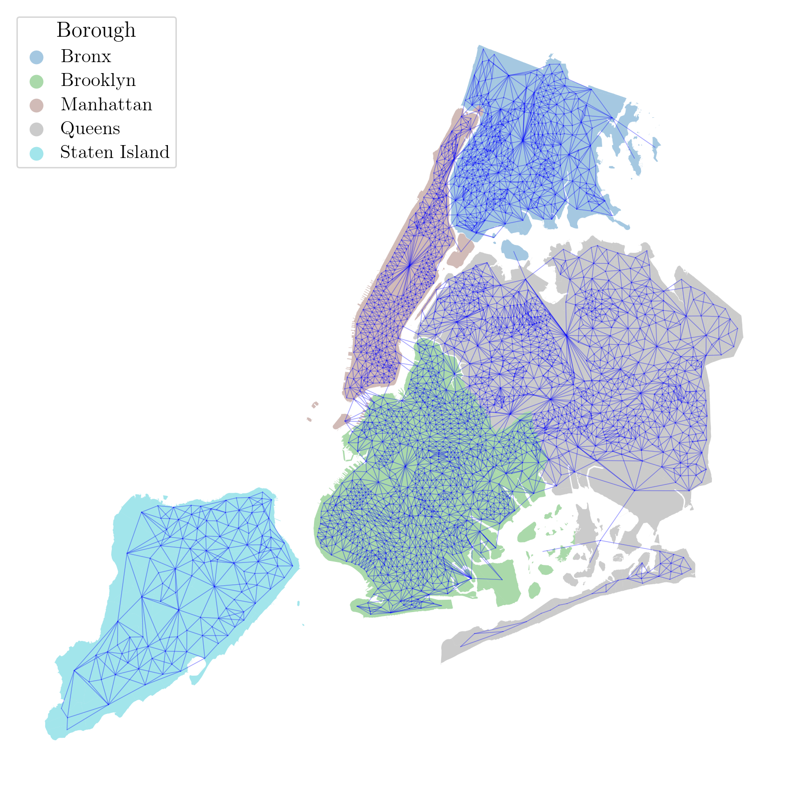
Census tract adjacency matrix.
We describe our approach in assessing adjacent Census tracts in New York City, as the city’s topography and dense development have produced intricate Census geographies. Further, with the flooding-oriented nature of our work, the accuracy of spatial adjacency relationships is important.
We use the water-clipped version of the 2020 NYC Census tracts, provided by the NYC Department of City Planning (NYC DCP, 2025). Using tracts with water areas included creates inaccurate adjacency relationships, such as tracts in Downtown Manhattan being neighbors to Governor’s Island. We generate neighbor relationships through geometric processing; we buffer (expand) each tract by 500 feet, and then assign adjacency between tracts that intersect. We visualize our adjacency matrix in Figure S1.
311 reports.
We denote the following complaint types as flooding-related for the purposes of our analysis: sewer backup, street flooding, catch basin clogged/flooded, manhole overflow, and highway flooding. We include reports from the entire day of September 29, 2023. The frequency of flooding-related 311 reports (see Figure S2) corresponds with the progress of the storm event (NYC Comptroller, 2024) .
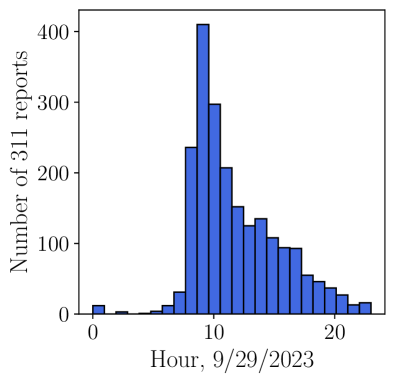
Elevation data.
We downsample the 1-foot Digital Elevation Model of NYC by a factor of 10 because it accelerates performance without significantly compromising accuracy at the granularity of a Census tract.
Appendix B Additional VLM details
B.1. Measurement of VLM performance
For all VLMs, including baseline models, we measure performance on our primary dataset by manually annotating a random subset of classified positives and a random subset of classified negatives. For our preferred VLM, we additionally assess performance on three additional days (as described in §3.1) by manually annotating 250 randomly-sampled classified negatives and 250 randomly-sampled classified positives (or, in cases where there are fewer than 250 classified positives, all classified positives) – see Table S2.
We only annotate an image as flooded if it unambiguously shows flooding. In very rare cases, technical artifacts render this ambiguous, including cases where (a) the view of the forthcoming street is obscured by the vehicle dashboard or (b) the dashcam is mispositioned, producing images that do not depict any part of the street; we mark these as negative. We similarly annotate images with visually ambiguous flooding (e.g., ambiguous reflections from sunlight) as negative.
| 9/29/23 | 12/18/23 | 1/10/24 | 2/10/24 | |
|---|---|---|---|---|
| New York | New York | New York | San Francisco | |
| 0.658 | 0.702 | 0.812 | 0.143 | |
| 0.006 | 0.000 | 0.000 | 0.000 |
B.2. VLM baselines
We compare the performance of our preferred VLM (Cambrian-13B) to several alternate VLM architectures with zero-shot prompting: CLIP; DeepSeek’s Janus Pro VLM; and Cambrian-1-8B. For all baselines, we experiment with multiple prompts and report the highest-performing configuration for each VLM in Table 1. Our preferred model achieves superior performance to the baselines. We estimate performance of each baseline by sampling a random subset of 250 classified positives, and 250 classified negatives, and obtaining ground-truth manual annotations.
We also compared our zero-shot prompting method to a supervised learning approach using noisy labels. Specifically, we first used CLIP (zero-shot) to identify candidate flooded images; then used GPT-4V (zero-shot) to further filter down the set, producing a set of noisy positives; and then fine-tuned a ResNet to distinguish between the noisy positives and all other images. (We did not use GPT-4V to annotate all images because it would impose a prohibitive cost on a dataset of our size.) We found that this method achieved inferior performance to our preferred approach (Table 1) at the cost of considerable additional complexity, and thus did not pursue it further.
B.3. Alternate VLM prompts
For each VLM we test, we assess multiple prompts and report results from the one which yields optimal performance. For the VLM we used for our primary analysis, Cambrian-13B, we compared performance of two prompts: (a) Does the street in this image show more than a foot of standing water? and (b) Does this image show a flooded street? We found that the latter prompt classified many more images as positive, resulting in slightly higher recall but much lower precision, and thus used the former.
Appendix C Additional Bayesian modeling details
C.1. Model priors
We place the following weakly informative priors on model parameters:
The negative-centered prior on reflects the prior belief that most locations are not flooded. We place an ordered vector constraint on to enforce the assumption that .
Our model of also includes an ICAR spatial component :
ICAR models are commonly used to capture spatially correlated data. We implement the ICAR component, as is standard, by incrementing the log probability using the the pairwise difference formula (Morris et al., 2019):
where denotes the adjacency matrix for Census areas. We place a soft sum-to-zero constraint on . We place a prior on the standard deviation of the ICAR component, .
C.2. Flooding features used in Bayesian model
As an input to our Bayesian model (i.e., in the notation above), we use 6 flood features from the external datasets described in §3.2: the number of 311 reports in a Census tract, the number of FloodNet sensors in a tract, the minimum elevation of the tract, the mean elevation of the tract, and the fraction of the tract with shallow and deep flooding in New York City Department of Environmental Protection Stormwater maps. We log-transform all right-skewed features, and z-score all features, prior to using them as inputs to the model, as is standard (Friedman, 2009).
C.3. Comparison of Bayesian model to baselines
As described in §5.1, we show that our Bayesian approach improves predictions of where flooded images will occur on a held-out test set, relative to both simple heuristics (e.g., the fraction of images which are classified as positive by the VLM) and machine learning baselines. We describe these baselines below.
C.3.1. Heuristic baselines
We compare to five heuristic baselines:
-
•
Fraction of positive classifications: i.e., the fraction of images in a Census tract which the VLM classifies as positive.
-
•
Any positive classifications: 1 if the VLM classifies any images in a Census tract as positive, 0 otherwise.
-
•
Number of positive classifications: the number of images in a tract the VLM classifies as positive.
-
•
Any positive ground-truth annotations: 1 if there are any images in a Census tract with ground-truth annotations as positive, 0 otherwise.
-
•
Number of positive annotations: the number of images in a tract with ground-truth positive annotations.
We do not use the fraction of positive ground-truth annotations as a baseline because most tracts have no ground-truth annotations at all and for them this baseline is not well-defined.
C.3.2. Supervised learning baselines
For the supervised learning baselines, we use the same set of flood-relevant features which are inputs to our Bayesian model (§C.2) to predict (a) the fraction of positive classifications and (b) the number of positive ground-truth annotations. We treat the variable to be predicted as a hyperparameter and report the setting which yields the best performance. We report results from both a linear regression model and a random forest model.
C.3.3. Graph smoothing baselines
We compare to graph Laplacian smoothing baselines, which use the graph Laplacian (where is the diagonal degree matrix, and is the adjacency matrix) to iteratively smooth a graph (Li et al., 2018a; Chen et al., 2019). One iteration of the algorithm updates the value x at each node (in our case, a Census tract) using the following diffusion update: , where is a step size parameter. The hyperparameters are , the number of smoothing iterations, and the initial value to be smoothed (fraction of positive classifications or number of positive ground-truth annotations); we report the hyperparameter configuration which maximizes performance.
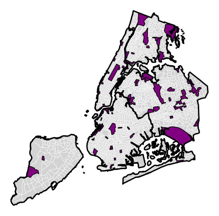
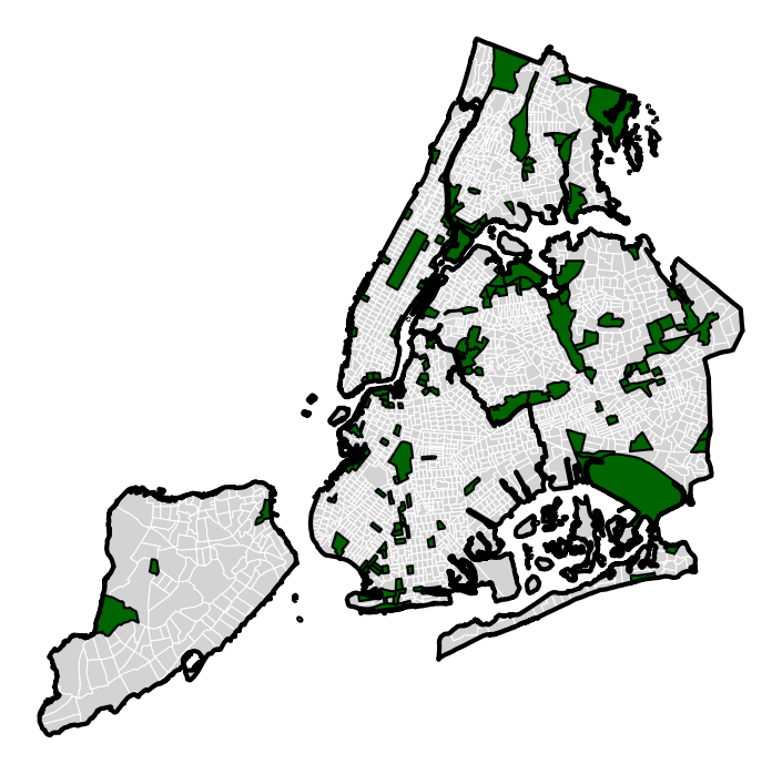
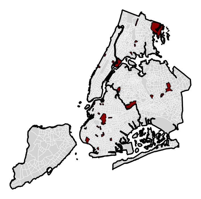
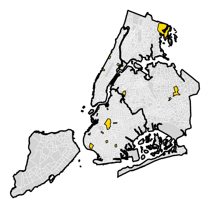
C.3.4. Comparison of baseline and Bayesian model performance
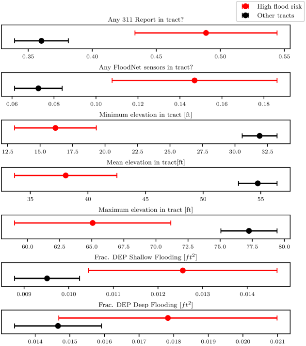
As described in §5.1, we compare the performance of our Bayesian model to that of baselines by partitioning the classified images into a train set (which we use to fit the Bayesian model and the baselines on the classifications) and a test set (which we use to assess out-of-sample performance). The inputs to the Bayesian model and the baselines are the number of images in each Census tract with a given ground-truth annotation (positive, negative, or unknown) and a given VLM classification (positive or negative), as well as the flood-risk features ; some baselines make use of only a subset of this information. Neither the Bayesian model nor the baselines make use of the raw images themselves.
We use multiple metrics to compare the performance of our Bayesian model to baselines. First, we assess the out-of-sample Pearson correlation with fraction of images in the tract which are classified flooded. For this task, the output from our Bayesian model that we use is , since this captures the fraction of images in a Census tract which are flooded.
We also assess the AUC in predicting whether (1) a Census tract will have any classified flooded images and (2) a Census tract will have any ground-truth annotated flooded images. For both these tasks, the output from our Bayesian model that we use is , since the goal is to predict the existence of a single image (as opposed to the fraction of flooded images).
On all of these metrics, our Bayesian model outperforms all baselines (Table 2).