Testing Conditional Stochastic Dominance at Target Points

Abstract

This paper introduces a novel test for conditional stochastic dominance (CSD) at specific values of the conditioning covariates, referred to as target points. The test is relevant for analyzing income inequality, evaluating treatment effects, and studying discrimination. We propose a Kolmogorov-Smirnov-type test statistic that utilizes induced order statistics from independent samples. Notably, the test features a data-independent critical value, eliminating the need for resampling techniques such as the bootstrap. Our approach avoids kernel smoothing and parametric assumptions, instead relying on a tuning parameter to select relevant observations. We establish the asymptotic properties of our test, showing that the induced order statistics converge to independent draws from the true conditional distributions and that the test controls asymptotic size under weak regularity conditions. While our results apply to both continuous and discrete data, in the discrete case, the critical value only provides a valid upper bound. To address this, we propose a refined critical value that significantly enhances power, requiring only knowledge of the support size of the distributions. Additionally, we analyze the test’s behavior in the limit experiment, demonstrating that it reduces to a problem analogous to testing unconditional stochastic dominance in finite samples. This framework allows us to prove the validity of permutation-based tests for stochastic dominance when the random variables are continuous. Monte Carlo simulations confirm the strong finite-sample performance of our method.

KEYWORDS: stochastic dominance, regression discontinuity design, induced order statistics, rank tests, permutation tests.

JEL classification codes: C12, C14.

1 Introduction

The concept of stochastic dominance has long been central to numerous areas of applied research, including investment strategies, income inequality analysis, and testing the distributional effects of public policies. This paper examines a specific aspect of stochastic dominance: testing conditional stochastic dominance (CSD) at specific values of the conditioning covariate, referred to as target points. Such conditional comparisons are crucial in many contexts, including evaluating treatment effects in social programs within a regression discontinuity design, analyzing economic disparities across demographic groups, and investigating potential discrimination in decision-making processes.

Unconditional stochastic dominance methods, which analyze entire distributions, have been extensively studied and widely applied in the literature, with foundational contributions dating back to Hodges (1958) and McFadden (1989) and more recent developments in Abadie (2002); Barrett and Donald (2003); Linton et al. (2005), and Linton et al. (2010), among others. However, in many empirical settings, the primary interest lies not in overall dominance but in dominance conditional on a subset of the population defined by specific characteristics or values of a conditioning variable. For instance, in regression discontinuity designs, the nature of the methodology necessitates comparing outcome distributions conditional on the cutoff of the running variable (Shen (2019); Qu and Yoon (2019); Shen and Zhang (2016); Donald et al. (2012)). Likewise, in wage discrimination studies, researchers may seek to compare wage distributions across demographic groups while controlling for observed skill levels (Becker (1957); Canay et al. (2024); Bharadwaj et al. (2024)).

The primary goal of this paper is to test whether the conditional cumulative distribution function (cdf) of one variable stochastically dominates that of another at specific values of a conditioning variable. Formally, we consider the null hypothesis

$$H_{0}:F_{Y}(t|z)\leq F_{X}(t|z)\quad\text{for all }(t,z)\in\mathbf{R}\times\mathcal{Z}~,$$

against the alternative that there exists some $(t,z)$ for which the reversed inequality holds strictly. Here, $F_{Y}(t|z)$ and $F_{X}(t|z)$ represent the conditional cdfs of the random variables $Y$ and $X$, respectively, given $Z=z$. Importantly, we focus on situations where the set of target values, $\mathcal{Z}$, is not the entire support of $Z$, but rather a finite collection of points (including the case of a singleton). To address this testing problem, we propose a novel procedure that leverages induced order statistics based on independent samples from $Y$ and $X$. Our test statistic, a Kolmogorov-Smirnov-type measure, captures the maximal deviation between the empirical cdfs of the two samples, conditional on observations near the target points. Crucially, the critical value we propose is derived in a deterministic, non-data-dependent manner once a tuning parameter is accounted for, ensuring computational simplicity.

Our contributions in this paper are both methodological and theoretical. First, we introduce a novel test for CSD at target points, which is particularly suited for settings where researchers seek to compare distributions conditional on covariates at specific values of the conditioning covariates. The proposed test exploits induced order statistics, leveraging observations closest to the target conditioning point to construct empirical cdfs that form the basis of our test statistic. Unlike traditional methods, our approach neither relies on kernel smoothing nor imposes parametric assumptions on conditional distributions. However, it does require a tuning parameter, which serves a role analogous to bandwidth selection in nonparametric estimation.

Second, we establish the asymptotic properties of our test, proving that it controls size in large samples under weak regularity conditions. We do this by showing that our test statistic converges to a limiting experiment, where the induced order statistics behave as independent draws from the true conditional distributions at the target point. This convergence allows us to derive a critical value that remains valid without relying on resampling techniques, such as the bootstrap. The regularity conditions we impose are mild, permitting the conditional distributions at the target point to have finitely many discontinuities. In contrast, related methods that test conditional stochastic dominance (CSD) in regression discontinuity designs (Shen (2019); Qu and Yoon (2019), and Shen and Zhang (2016)) assume continuous conditional distributions at the target point. This continuity assumption can be restrictive in many empirically relevant contexts. For example, income distributions often exhibit point masses at tax brackets, and wage distributions at the minimum wage. Additionally, our regularity conditions only require the conditional distributions $F_{Y}(t|z)$ and $F_{X}(t|z)$ to be continuous in $z$ at the target points, uniformly over $t$. In contrast, these existing methods, which rely on conventional nonparametric estimators, require stronger regularity conditions, such as twice-differentiability of the conditional distributions in the conditioning variable.

Third, we show that the proposed critical value aligns with the one obtained from a permutation-based approach when the random variables $Y$ and $X$ are both continuous, thus establishing a natural connection between our method and the broader literature on rank-based inference. To the best of our knowledge, this result provides the first formal justification for the validity of permutation-based inference in testing stochastic dominance relationships. We demonstrate that the critical value of our test cannot be improved when both $Y$ and $X$ are continuous. However, we recognize that this result does not extend to the case when either $Y$ or $X$ is discretely distributed. For this latter case, we introduce a refined critical value, which is typically smaller than the default one we propose and is only a function of the support points for the random variables $Y$ and $X$. This refinement enhances power relative to the default critical value, though it comes at the cost of increased computational complexity.

Finally, we explore the finite-sample performance of our test through Monte Carlo simulations and provide data-dependent rules for selecting the key tuning parameters, offering practical guidance for empirical researchers seeking to implement our test.

Our work contributes to the extensive literature on stochastic dominance testing, building on seminal contributions such as Anderson (1996); Davidson and Duclos (2000); Abadie (2002); Barrett and Donald (2003); Linton et al. (2005), and Linton et al. (2010), among others. While these studies predominantly rely on asymptotic arguments and resampling techniques, our approach to testing CSD differs in that, in the limit experiment, the conditional testing problem simplifies to a finite-sample unconditional testing problem. In the context of CSD testing, prior research — including Delgado and Escanciano (2013); Gonzalo and Olmo (2014); Chang et al. (2015), and Andrews and Shi (2017) — has developed methodologies for assessing stochastic dominance over a range or across the entire support of a continuous conditioning variable $Z$. Our work diverges from this literature by targeting CSD at specific target points rather than over broad intervals. A distinct line of research, including Donald et al. (2012); Shen and Zhang (2016); Shen (2019), and Qu and Yoon (2019), examines stochastic dominance testing within regression discontinuity designs, where dominance is conditional on cutoffs. While these approaches assume continuity in conditional distributions, our method is more flexible, accommodating distributions with finitely many discontinuities. Furthermore, by leveraging properties of induced order statistics, we eliminate the need for smoothing techniques, resulting in a novel yet computationally simple testing procedure.

Our work closely aligns with the well-established literature on testing the equality of two distributions. Foundational contributions by Gnedenko and Koroluk (1951), Korolyuk (1955), and Blackman (1956) established that the finite-sample distribution of the one-sided Kolmogorov-Smirnov test statistic is pivotal when both distribution functions are continuous, deriving closed-form expressions under various simplifying assumptions. Later research by Hodges (1958); Hájek and Šidák (1967), and Durbin (1973a) developed methods to approximate this finite-sample distribution. Although our null hypothesis differs, our critical value coincides with the corresponding quantile of this distribution. Notably, Hodges (1958) and McFadden (1989) proposed that the one-sided Kolmogorov-Smirnov test, originally designed for testing equality of two distributions, could be adapted to test stochastic dominance under continuity assumptions — though without formal proof. We provide a rigorous justification for this claim.

The remainder of the paper is organized as follows. Section 2 formally defines the testing problem and introduces the necessary notation. Section 3 presents the induced order statistics that form the basis of our test and introduces the proposed critical value. Section 4 establishes the asymptotic properties of our test, demonstrating that in the limit experiment, the induced order statistics behave as independent draws from the true conditional distributions at the target points. We then prove that our test controls the rejection probability under the null hypothesis in large samples. Section 5 discusses additional refinements and extensions, including a data-dependent rule for selecting tuning parameters and an improved version of the test that enhances power when the random variables $Y$ and $X$ are discrete. Section 6 evaluates the finite-sample performance of our test through Monte Carlo simulations. Finally, Section 7 concludes with remarks on possible directions for future research.

2 Testing problem

Let $(X,Y,Z)$ be random variables with distribution $P$ taking values in $\mathbf{R}^{3}$. Define the cdfs of $Y$ and $X$ given $Z$ as follows:

$$F_{Y}(t|z)=P\{Y\leq t\mid Z=z\}\quad\text{and}\quad F_{X}(t|z)=P\{X\leq t\mid Z=z\}~.$$

We are interested in testing the null hypothesis:

$$H_{0}:F_{Y}(t|z)\leq F_{X}(t|z)\text{ for all }(t,z)\in\mathbf{R}\times\mathcal{Z}$$ (1)

versus the alternative hypothesis:

$$H_{1}:F_{Y}(t|z)>F_{X}(t|z)\text{ for some }(t,z)\in\mathbf{R}\times\mathcal{Z}~,$$

where $\mathcal{Z}=\{z_{1},\dots,z_{L}\}$ is a finite set of target conditional points. The case where $L=1$ and $Z$ is a continuously distributed random variable is both simpler and particularly relevant in empirical applications. To minimize notational clutter, we focus on this case for the remainder of the paper, with Section 5.4 addressing the case where $L>1$.

The null hypothesis in (1) states that the distribution of $Y$ conditional on $Z=z$ stochastically dominates the distribution of $X$ conditional on $Z=z$. Using the notation $Y\succ_{z}^{1}X$ to denote first-order stochastic dominance conditional on $Z=z$, we can rewrite the null hypothesis more compactly as:

$$H_{0}:Y\succ_{z}^{1}X\text{ for all }z\in\mathcal{Z}~.$$ (2)

To test this hypothesis, we assume the analyst observes two independent samples. The first sample consists of $n_{y}$ i.i.d. observations from the joint distribution of $(Y,Z)$, which we refer to as the $Y$-sample. The second sample consists of $n_{x}$ i.i.d. observations from the joint distribution of $(X,Z)$, which we refer to as the $X$-sample. Specifically, the observed data are given by:

$$\{(Y_{i},Z_{i}):1\leq i\leq n_{y}\}\text{ and }\{(X_{j},Z_{j}):1\leq j\leq n_{x}\}~.$$ (3)

3 Test based on induced ordered statistics

Let the observed data be the one given in (3). Let $(q_{y},q_{x})$ be two small positive integers (relative to $(n_{y},n_{x})$) and consider the point $z_{0}\in\mathcal{Z}$. The test we propose is based on the following two samples:

• The $q_{y}$ values of $\{Y_{i}:1\leq i\leq n_{y}\}$ associated with the $q_{y}$ values of $\{Z_{i}:1\leq i\leq n_{y}\}$ closest to $z_{0}$, and

• The $q_{x}$ values of $\{X_{i}:1\leq i\leq n_{x}\}$ associated with the $q_{x}$ values of $\{Z_{i}:1\leq i\leq n_{x}\}$ closest to $z_{0}$.

To define these samples formally, we introduce $g$-order statistics for the conditioning variable $Z$, where $g(Z):=|Z-z_{0}|$; see Reiss (1989, Section 2.1) and Kaufmann and Reiss (1992). For any two values $z,z^{\prime}\in\mathcal{Z}$, we define the ordering $\leq_{g}$ as follows:

$$z\leq_{g}z^{\prime}\quad\text{if and only if}\quad g(z)\leq g(z^{\prime})~.$$

This defines a $g$-ordering on the set $\mathcal{Z}$. The $g$-order statistics $Z_{g,(i)}$ are then the values of $Z$ ordered according to this criterion:

$$Z_{g,(1)}\leq_{g}Z_{g,(2)}\leq_{g}\cdots\leq_{g}Z_{g,(n)}~,$$

see, e.g., Reiss (1989); Kaufmann and Reiss (1992); Bugni and Canay (2021).

We then take the values of $\{Y_{i}:1\leq i\leq n_{y}\}$ associated with the $q_{y}$ smallest $g$-ordered statistics of $Z$ in the $Y$-sample, denoted by

$$Y_{n_{y},[1]},Y_{n_{y},[2]},\dots,Y_{n_{y},[q_{y}]}~.$$ (4)

That is, $Y_{n_{y},[j]}=Y_{k}$ if $Z_{g,(j)}=Z_{k}$ for $k=1,\dots,q_{y}$. Similarly, we take the values of $\{X_{i}:1\leq i\leq n_{x}\}$ associated with the $q_{y}$ smallest $g$-ordered statistics of $Z$ in the $X$-sample, denoted by

$$X_{n_{x},[1]},X_{n_{x},[2]},\dots,X_{n_{x},[q_{x}]}~.$$ (5)

The random variables in (4) and (5) are referred to as induced order statistics or concomitants of order statistics; see David and Galambos (1974); Bhattacharya (1974); Canay and Kamat (2018). Intuitively, we view these samples as independent samples of $Y$ and $X$, conditional on $Z$ being “close” to $z_{0}$. A key feature of the test we propose is that it relies solely on these two sets of induced order statistics, without depending on the rest of the observed data. Specifically, if we let $n:=n_{y}+n_{x}$ and $q:=q_{y}+q_{x}$, the effective (pooled) sample is given by

$$S_{n}=(S_{n,1},\dots,S_{n,q}):=(Y_{n_{y},[1]},\dots,Y_{n_{y},[q_{y}]},X_{n_{x},[1]},\dots,X_{n_{x},[q_{x}]})~.$$ (6)

Thus, our test is entirely based on $S_{n}$. It is also important to note that the first $q_{y}$ elements of $S_{n}$ are associated with the $Y$-sample, while the remaining $q_{x}$ elements correspond to the $X$-sample.

Having defined the induced order statistics, we can now define our test statistic as

$$T(S_{n})=\sup_{t\in\mathbf{R}}\left(\hat{F}_{n,Y}(t)-\hat{F}_{n,X}(t)\right)=\max_{k\in\{1,\dots,q_{y}\}}\left(\hat{F}_{n,Y}(S_{n,k})-\hat{F}_{n,X}(S_{n,k})\right)~,$$ (7)

where the empirical cdfs are,

$$\hat{F}_{n,Y}(t):=\frac{1}{q_{y}}\sum_{j=1}^{q_{y}}I\{S_{n,j}\leq t\}\quad\text{ and }\quad\hat{F}_{n,X}(t):=\frac{1}{q_{x}}\sum_{j=1}^{q_{x}}I\{S_{n,q_{y}+j}\leq t\}~.$$ (8)

The test statistic in (7) is a one-sided Kolmogorov-Smirnov (KS) test statistic, see Hajek et al. (1999, p. 99), and the test we propose rejects the null hypothesis in (2) for large values of $T(S_{n})$.

Finally, to introduce the critical value let $\alpha\in(0,1)$ be given and $\{U_{j}:1\leq j\leq q\}$ be a sequence of uniform random variables i.i.d., that is, $U_{j}\sim U[0,1]$. Define $\Delta(u)$ as

$$\Delta(u):=\frac{1}{q_{y}}\sum_{j=1}^{q_{y}}I\{U_{j}\leq u\}-\frac{1}{q_{x}}\sum_{j=q_{y}+1}^{q}I\{U_{j}\leq u\}~,$$ (9)

and

$$c_{\alpha}(q_{y},q):=\inf_{x\in\mathbf{R}}\left\{P\left\{\sup_{u\in(0,1)}\Delta(u)\leq x\right\}\geq 1-\alpha\right\}~.$$ (10)

The test we propose for the null hypothesis in (2) is

$$\phi(S_{n}):=I\{T(S_{n})>c_{\alpha}(q_{y},q)\}~.$$ (11)

We reiterate that (11) corresponds to our test with a single target point ($L=1$). Section 5 extends this framework to the general case with multiple target points ($L>1$).

There are several important features of the test $\phi(S_{n})$ in (11) worth highlighting. First, our formal results extend to other choices of test statistics $T:\mathbf{R}^{q}\to\mathbf{R}$, provided these statistics are invariant to rank-preserving transformations, i.e., they depend only on the order of elements in $S_{n}$. This includes the one-sided Cramér-von Mises (CvM) test statistic,

$$T(S_{n})=\int\left(\hat{F}_{n,Y}(s)-\hat{F}_{n,X}(s)\right)^{+}d\hat{F}_{n,S}(s)=\frac{1}{q}\sum_{j=1}^{q}\left(\hat{F}_{n,Y}(S_{n,j})-\hat{F}_{n,X}(S_{n,j})\right)^{+}~,$$ (12)

where $\hat{F}_{n,S}(s)$ denotes the empirical cdf of $S_{n}$ and $x^{+}=\max\{x,0\}^{2}$. The one-sided Anderson-Darling (AD) test statistic is also included:

$$T(S_{n})=\int\frac{\left(\hat{F}_{n,Y}(s)-\hat{F}_{n,X}(s)\right)^{+}}{\hat{F}_{n,S}(s)(1-\hat{F}_{n,S}(s))}d\hat{F}_{n,S}(s)=\frac{1}{q}\sum_{j=1}^{q}\frac{\left(\hat{F}_{n,Y}(S_{n,j})-\hat{F}_{n,X}(S_{n,j})\right)^{+}}{\hat{F}_{n,S}(S_{n,j})\left(1-\hat{F}_{n,S}(S_{n,j})\right)}~.$$ (13)

These statistics align with their standard textbook definitions, as discussed in Hajek et al. (1999, p. 101), and are solely functions of $S_{n}$. Although we focus primarily on the KS statistic in (7) for ease of exposition, our results do not favor this test statistic over others. Second, the critical value $c_{\alpha}(q_{y},q)$ is straightforward to compute and cannot be improved asymptotically when $Y$ and $X$ are continuously distributed. However, for discrete random variables with limited support, this critical value can be improved, and we discuss how to do so in Section 5.2.

Remark 3.1.

From a computational perspective, there are two notable aspects of the test $\phi(S_{n})$. First, the supremum over $\mathbf{R}$ in (7) can be replaced by a maximum over the set $\{1,\dots,q_{y}\}$. This simplification arises because the KS test statistic increases only when evaluated at points corresponding to the $Y$-sample, which are the first $q_{y}$ elements in the vector $S_{n}$. Consequently, the supremum in the definition of $c_{\alpha}(q_{y},q)$ can also be replaced with a maximum over $\{1,\dots,q_{y}\}$. This allows the critical value $c_{\alpha}(q_{y},q)$ to be computed with arbitrary accuracy through simulation.  ∎

Remark 3.2.

When the random variables $Y$ and $X$ are continuously distributed, we demonstrate in Section 5.3 that the critical value $c_{\alpha}(q_{y},q)$ is asymptotically equivalent to the quantile of the permutation distribution of the test statistic. This equivalence extends to the analytical (finite-sample) quantile of $T(S_{n})$ in the limit experiment. However, this analogy does not hold when $Y$ or $X$ are discretely distributed.  ∎

Remark 3.3.

The values of $(q_{y},q_{x})$ are tuning parameters chosen by the researcher. In Section 5.1, we provide data-dependent guidelines for selecting these values and evaluate their performance through simulations presented in Section 6.  ∎

Remark 3.4.

As mentioned in the introduction, one natural application of our test is in the context of a sharp regression discontinuity design, where an outcome $\tilde{Y}$ depends on a running variable $\tilde{Z}$, and the point of interest is the discontinuity at $z_{0}$. The observed sample in this case is $\{(\tilde{Y}_{i},\tilde{Z}_{i}):1\leq i\leq n\}$, and the two samples needed for implementing our test are defined as follows:

$$\{(Y_{i},Z_{i}):1\leq i\leq n_{y}\}:=\{(\tilde{Y}_{i},\tilde{Z}_{i}):1\leq i\leq n\text{ such that }Z_{i}\leq z_{0}\}~,$$

and

$$\{(X_{i},Z_{i}):1\leq i\leq n_{x}\}:=\{(\tilde{Y}_{i},\tilde{Z}_{i}):1\leq i\leq n\text{ such that }Z_{i}>z_{0}\}~.$$

Importantly, this formulation shows that the point $z_{0}$ can be either an interior or a boundary point in its support.  ∎

4 Asymptotic framework and formal results

In this section, we examine the asymptotic properties of the test in (11) within a framework where $q:=q_{y}+q_{x}$ is fixed and $n\to\infty$, where $n\to\infty$ is understood as $\min\{n_{y},n_{x}\}\to\infty$. This involves two steps: first, we establish the asymptotic properties of induced order statistics in (6), enabling us to prove a main theorem that links the finite-sample properties of $\phi(S_{n})$ to those of the same test in the limit experiment. We then explore the properties of our test in the limit experiment and make connections to natural alternatives, including permutation tests.

4.1 Asymptotic validity of the new test

We start by deriving a result on the induced order statistics collected in the vector $S_{n}$ in (6). In order to do so, we make the following assumptions.

Assumption 4.1.

For any $\varepsilon>0$ and $z\in\mathcal{Z}$, $P\{Z\in(z-\varepsilon,z+\varepsilon)\}>0$.

Assumption 4.2.

For any $z\in\mathcal{Z}$ and sequence $z_{k}\to z$, $\sup_{t\in\mathbf{R}}|F_{Y}(t|z_{k})-F_{Y}(t|z)|\to 0$ and $\sup_{t\in\mathbf{R}}|F_{X}(t|z_{k})-F_{X}(t|z)|\to 0$.

Assumption 4.1 requires that the distribution of $Z$ is locally dense at each of the points in $\mathcal{Z}$. Note that this includes the case where $Z$ has a mass point at $z\in\mathcal{Z}$. Assumption 4.2 is a smoothness assumption required to guarantee that conditioning on observations close to $z$ is informative about the distribution conditional on $Z=z$.

Theorem 4.1.

Let Assumptions 4.1 and 4.2 hold. Then,

$$S_{n}\stackrel{{\scriptstyle d}}{{\to}}S=(S_{1},\dots,S_{q})~,$$ (14)

where for any $s:=(s_{1},\dots,s_{q})\in\mathbf{R}^{q}$, the random vector $S$ satisfies

$$P\{S\leq s\}=\prod_{j=1}^{q_{y}}F_{Y}(s_{j}|z_{0})\cdot\prod_{j=q_{y}+1}^{q}F_{X}(s_{j}|z_{0})~.$$

Theorem 4.1 is a special case of Theorem B.1 in Appendix B when $L=1$, which in turn is a generalization of Canay and Kamat (2018, Theorem 4.1) for the case where there are multiple conditioning values. It establishes that the limiting distribution of the induced order statistics in the vector $S_{n}$ is such that the elements of the vector, denoted by $S$, are mutually independent. In addition, the first $q_{y}$ elements of this vector follow the distribution $F_{Y}(s_{j}|z_{0})$, while the remaining $q_{x}$ elements follow $F_{X}(s_{j}|z_{0})$. The proof leverages the fact that the induced order statistics $S_{n}$ in (6) are conditionally independent given $(Z_{1},\dots,Z_{n})$, with conditional cdfs

$$F_{Y}(s|{Z_{n_{y},(q_{y})}}),\dots,F_{Y}(s|{Z_{n_{y},(1)}}),F_{X}(s|{Z_{n_{x},(q_{x})}}),\dots,F_{X}(s|{Z_{n_{x},(1)}})~.$$

The result then follows by showing that $Z_{n_{y},(j)}\overset{p}{\to}z_{0}$ and $Z_{n_{x},(j)}\overset{p}{\to}z_{0}$ for all $j\in\{1,\dots,q\}$, and invoking standard properties of weak convergence. This intermediate result plays a crucial role in the proof of Theorem 4.2 presented in the next section.

In addition to Assumptions 4.1 and 4.2, we also require that the random variables $Y$ and $X$ have, conditional on $Z=z$, distributions with at most a finite number of discontinuity points. To state this assumption formally, let $\mathcal{D}_{Y}(z)$ and $\mathcal{D}_{X}(z)$ denote the sets of discontinuity points of the cdfs of ${Y|Z=z}$ and ${X|Z=z}$, respectively.

Assumption 4.3.

For any $z\in\mathcal{Z}$, $|\mathcal{D}_{Y}(z)|$ and $|\mathcal{D}_{X}(z)|$ are finite.

It is important to note that Assumption 4.3 allows both $Y$ and $X$ to be continuous, discrete, or mixed random variables. However, it excludes cases where these variables have countably many discontinuities conditional on $z\in\mathcal{Z}$. We also point out that Theorem 4.1 does not require Assumption 4.3.

We now formalize our main result in Theorem 4.2, which shows that the test defined in (11) is asymptotically level $\alpha$ under the assumptions we just introduced. We denote by $\mathbf{P}$ the space of distributions for $P$ that satisfy the stated assumptions, and by

$$\mathbf{P}_{0}:=\{P\in\mathbf{P}:\eqref{eq:H0}~\text{holds}\}$$ (15)

the subset of distributions $P\in\mathbf{P}$ satisfying the null hypothesis in (1). Finally, we denote by $E_{P}[\cdot]$ the expected value with respect to the distribution $P$.

Theorem 4.2.

Let Assumptions 4.1, 4.2 and 4.3 hold. Let $\alpha\in(0,1)$ be given, $T$ be the KS test statisic in (7), and $\phi(\cdot)$ be the test in (11). Then,

$$\limsup_{n\to\infty}E_{P}[\phi(S_{n})]\leq\alpha$$ (16)

whenever $P\in\mathbf{P}_{0}$.

Theorem 4.2 establishes the asymptotic validity of the test in (11). As mentioned earlier, the result accommodates the cases where $Y$ and $X$ can be continuous, discrete, or mixed random variables. However, there are three main reasons why the inequality in (16) may be strict, resulting in an asymptotic size strictly below $\alpha$. First, for distributions $P$ in the interior of $\mathbf{P}_{0}$, where the inequality in (1) holds strictly for some $t\in\mathbf{R}$, the test is expected to reject with probability less than $\alpha$, with a magnitude depending on the “distance” of $P$ from the boundary of $\mathbf{P}_{0}$. Second, in cases where $Y$ or $X$ are discretely distributed, the critical value defined in (10) serves as an upper bound for the desired quantile, as discussed further in Section 5.2. Finally, the test statistic $\Delta(u)$ in (9) is discretely distributed, and when $q$ is small, it may take only a limited number of distinct values. Consequently, the achieved significance level

$$\bar{\alpha}:=P\left\{\sup_{u\in(0,1)}\Delta(u)>c_{\alpha}(q_{y},q)\right\}$$ (17)

satisfies $\bar{\alpha}\leq\alpha$ by definition, but may be strictly less than $\alpha$. Whether $\bar{\alpha}=\alpha$ occurs or not depends on whether the critical value $c_{\alpha}(q_{y},q)$ aligns exactly with one of the discrete jumps in the cdf of $\sup_{u\in(0,1)}\Delta(u)$, which in turn depends on $\alpha$, $q_{y}$, and $q$.

5 Discussion and extensions

5.1 Data-dependent choice of tuning parameters

In this section, we discuss the practical considerations for implementing our test. The test requires two tuning parameters: $q_{y}$ and $q_{x}$. We propose a data-dependent method for selecting these values, drawing on arguments from Armstrong and Kolesár (2018), similar to the approach used by Bugni and Canay (2021) in their setting. This method leverages a bias-variance trade-off inherent in the estimation of the conditional cdfs used in the test statistic for $\phi(S_{n})$, within an asymptotic framework where $q$ can grow with $n$, albeit at a slow rate. Our goal is to provide practical guidance for selecting these tuning parameters based on the data, rather than claiming optimality of any sort. We examine the performance of this rule via Monte Carlo simulations in Section 6.

We propose choosing $q_{x}$ and $q_{y}$ using the following data-dependent rules:

$$q_{y}^{*}:=n_{y}^{1/2}\left(\frac{4\cdot\phi_{\mu_{Z},\sigma_{Z}}^{2}(z_{0})}{\frac{2}{\sigma_{Z}}\frac{1}{\sqrt{2\pi e}}+\frac{|\rho_{Y}|}{\sigma_{Z}\sqrt{1-\rho_{Y}^{2}}}\frac{1}{\sqrt{2\pi}}}\right)^{2/3}$$ (18)

and

$$q_{x}^{*}:=n_{x}^{1/2}\left(\frac{4\cdot\phi_{\mu_{Z},\sigma_{Z}}^{2}(z_{0})}{\frac{2}{\sigma_{Z}}\frac{1}{\sqrt{2\pi e}}+\frac{|\rho_{X}|}{\sigma_{Z}\sqrt{1-\rho_{X}^{2}}}\frac{1}{\sqrt{2\pi}}}\right)^{2/3}~,$$ (19)

where $\mu_{Z}:=E[Z]$, $\sigma_{Z}^{2}:=\text{Var}[Z]$, $\phi_{\mu_{Z},\sigma_{Z}}(\cdot)$ denotes the probability density function of a normal distribution with mean $\mu_{Z}$ and variance $\sigma_{Z}^{2}$, and $\rho_{Y}$ and $\rho_{X}$ are the correlation coefficients between $Y$ and $Z$, and $X$ and $Z$, respectively.

In order to provide some intuition as to why this rule of thumb may be reasonable, assume that the random variable $Z$ is continuous with a density function $f_{Z}(\cdot)$ satisfying

$$|f_{Z}(z_{1})-f_{Z}(z_{2})|\leq C_{Z}|z_{1}-z_{2}|\text{ for a Lipschitz constant }C_{Z}<\infty~,$$

and any values $z_{1},z_{2}\in\mathcal{Z}$. In addition, suppose that the conditional cdf of $Y$ satisfies

$$\left|\frac{\partial F_{Y}(t|z)}{\partial z}\right|\leq C_{Y}\quad\text{ for a constant }C_{Y}<\infty~,$$

and that the conditional cdf of $X$ satisfies the same condition with a constant $C_{X}$. It can be shown that the standardized bias $B_{n_{y},q_{y}}$ associated with the estimator of the conditional cdf $F_{Y}(t|z_{0})$ satisfies

$$|B_{n_{y},q_{y}}|\leq\frac{q_{y}^{3/2}}{n_{y}}\frac{2C_{Z}+C_{Y}}{4f^{2}_{Z}(z_{0})}~.$$ (20)

Let $t^{\ast}$ denote the right-hand side of (20). Solving for $q_{y}$, we obtain

$$q_{y}=n_{y}^{2/3}(t^{\ast})^{2/3}\left(\frac{4f^{2}_{Z}(z_{0})}{2C_{Z}+C_{Y}}\right)^{2/3}~.$$

Thus, the data-dependent rule we propose in (18) and (19) can be interpreted as under-smoothed approximations of these values, where the unknown Lipschitz constants are approximated by the working model $Z\sim N(\mu_{Z},\sigma_{Z})$. The constant multiplying $n_{y}^{1/2}$ in (18) is intuitive for two reasons. First, it reflects the idea that a steeper density at $z_{0}$, or a steeper derivative of the conditional cdfs at $z_{0}$, should correspond to smaller values of $q_{y}$. Intuitively, when the density is steeper at $z_{0}$, using observations close to $z_{0}$ does not provide a good approximation to the quantities at $z_{0}$. Since the maximum slope is determined by the constants $C_{Z}$ and $C_{Y}$, the rule is inversely proportional to these constants. Second, the rule accounts for the idea that $q_{y}$ should be smaller when the density at $z_{0}$ is low. When $f_{Z}(z_{0})$ is small, the $q_{y}$ closest observations to $z_{0}$ are likely to be “far” from $z_{0}$. While one could replace the normality assumption with a non-parametric estimator of $f_{Z}(\cdot)$, it is unfortunately impossible to adaptively choose $C_{Z}$ and $C_{Y}$ for testing (2) (see, e.g., Armstrong and Kolesár, 2018). Since any data-dependent rule for $q$ requires a reference for $C_{Z}$ and $C_{Y}$, we prioritize simplicity and use normality for both $f_{Z}(\cdot)$ and the associated constants.

5.2 Refined critical value for discrete data

Recall that the critical value of the test $\phi(S_{n})$ in (11) was defined as

$$c_{\alpha}(q_{y},q):=\inf_{x\in\mathbf{R}}\left\{P\left\{\sup_{u\in(0,1)}\Delta(u)\leq x\right\}\geq 1-\alpha\right\}~,$$

where $\{U_{j}:1\leq j\leq q\}$ are i.i.d. uniform random variables and

$$\Delta(u):=\frac{1}{q_{y}}\sum_{j=1}^{q_{y}}I\{U_{j}\leq u\}-\frac{1}{q_{x}}\sum_{j=q_{y}+1}^{q}I\{U_{j}\leq u\}~,$$

was defined in (9). This critical value provides a valid (asymptotic) upper bound to the quantile of the test statistic $T(S_{n})$ and is shown to be equal to this quantile (in the limit experiment) whenever the random variables $Y$ and $X$ are both continuous and the null hypothesis in (1) holds with equality, see Section 5.3. However, when either $Y$ or $X$ is discretely distributed with a limited number of support points, it is possible to construct a smaller critical value than $c_{\alpha}(q_{y},q)$, which still controls the asymptotic size of the test, albeit at the cost of additional computational complexity.

Let $\mathbf{Y}$ and $\mathbf{X}$ denote the support of $Y$ and $X$, respectively. To understand the reasoning behind the refined critical value for discrete data, observe that in the proof of Theorem B.2, the probability

$$P\left\{\sup_{u\in\mathcal{U}}\Delta(u)>c_{\alpha}(q_{y},q)\right\}~,$$

where $\mathcal{U}:=\cup_{t\in\mathbf{Y}}\{u=F_{X}(t|z_{0})\}$ is the set of values that $F_{X}(t|z_{0})$ takes as $t$ varies over the support of $Y$, is bounded by

$$P\left\{\sup_{u\in\mathbf{(}0,1)}\Delta(u)>c_{\alpha}(q_{y},q)\right\}~.$$

This replacement of the set $\mathcal{U}$ with the entire interval $(0,1)$ leads to a critical value that may be unnecessarily large when $\mathcal{U}$ contains only a few points, that being because $\mathbf{Y}$ contains only a few points or because $F_{X}(t|z_{0})$ takes few distinct values as $t$ varies. In fact, the cardinality of the set $\mathcal{U}$ is determined by the smallest support size of $Y$ and $X$.

In order to define our refined critical value for discrete data, let $r$ denote the smallest support size of $Y$ and $X$, i.e.,

$$r:=\min\{|\mathbf{Y}|,|\mathbf{X}|\}~.$$

Let $\mathbf{U}_{r}$ denote the collection of all sets of $r$ distinct points in $(0,1)$. We denote an arbitrary element in $\mathbf{U}_{r}$ by

$$\mathcal{U}_{r}:=\{u_{1},u_{2},\dots,u_{r}:u_{i}\in(0,1)\text{ and }u_{i}\neq u_{i^{\prime}}\text{ for }i\neq i^{\prime}\}~.$$

With this notation, our refined critical value is defined as

$$c^{r}_{\alpha}(q_{y},q):=\inf_{x\in\mathbf{R}}\left\{\inf_{\mathcal{U}_{r}\in\mathbf{U}_{r}}P\left\{\sup_{u\in\mathcal{U}_{r}}\Delta(u)\leq x\right\}\geq 1-\alpha\right\}~,$$ (21)

with $\Delta(u)$ as in (9), and the refined test for the null hypothesis in (2) when either $Y$ or $X$ is discretely distributed with a limited number of support points is thus

$$\phi^{r}(S_{n}):=I\{T(S_{n})>c^{r}_{\alpha}(q_{y},q)\}~.$$ (22)

Section 5.4 presents the general version of this test for the case $L>1$.

The power advantages of using $c_{\alpha}^{r}(q_{y},q)$ over $c_{\alpha}(q_{y},q)$ are most pronounced when $r$ is small. Our numerical analysis shows the most significant gains when $r\leq 10$. Therefore, we emphasize that this refinement is specifically intended for discrete data with a limited number of support points, rather than for all discrete data. The computational cost of $c_{\alpha}^{r}(q_{y},q)$ is also increasing in $r$, and so as $r$ gets larger the cost is higher and the benefits are lower.

We propose to compute $c_{\alpha}^{r}(q_{y},q)$ numerically, by solving the following optimization problem:

$$c_{\alpha}^{r}(q_{y},q)=\min\left\{x\in[c_{\rm lb},c_{\rm ub}]\cap\mathbf{T}:\inf_{\mathcal{U}_{r}\in\mathbf{U}_{r}}P\left\{\max_{u\in\mathcal{U}_{r}}\Delta(u)\leq x\right\}~\geq 1-\alpha\right\}~,$$ (23)

where $\mathbf{T}$ is the support of $\Delta(u)$ in (9). Here, $c_{\rm ub}=c_{\alpha}(q_{y},q)$ and $c_{\rm lb}$ is given by

$$c_{\rm lb}:=\min_{x\in\mathbf{T}}\left\{P\left\{\max_{u\in\left\{\frac{1}{1+r},\frac{2}{1+r},\dots,\frac{r}{1+r}\right\}}\Delta(u)\leq x\right\}\geq 1-\alpha\right\}~.$$

The fact that $c_{\alpha}(q_{y},q)$ provides a valid upper bound should not be surprising given the preceding discussion. On the other hand, $c_{\rm lb}$ serves as a valid lower bound because $\left\{\frac{1}{1+r},\frac{2}{1+r},\dots,\frac{r}{1+r}\right\}$ is a specific element in $\mathbf{U}_{r}$. In our numerical evaluations, we often found that $c_{\alpha}^{r}(q_{y},q)=c_{\rm lb}$, but not always. This indicates that the additional optimization in (23) cannot be generally avoided. For modest values of $r$ and $q$, however, this optimization step is computationally straightforward, primarily due to the relatively small number of points typically found in $[c_{\rm lb},c_{\rm ub}]\cap\mathbf{T}$; see Remark 5.1.

Remark 5.1.

The support $\mathbf{T}$ of $\Delta(u)$ is a discrete subset of $[-1,1]$ and can be easily enumerated for modest values of $q$. Specifically, the support has cardinality bounded by $(q_{y}+1)(q_{x}+1)$, and it is independent of the realizations of the random variables as well as the specific value that $u\in(0,1)$ takes.  ∎

5.3 Properties of our test in the limit experiment

In this section, we study the properties of the test $\phi(\cdot)$ in (11) within the framework of the limit experiment. By Theorem 4.1, this test is equivalent to $\phi(S)$, where

$$S=(S_{1},S_{2},\dots,S_{q}),\quad S_{j}\sim F_{Y}(\cdot|z_{0})\text{ for }j\leq q_{y}\text{ and }S_{j}\sim F_{X}(\cdot|z_{0})\text{ for }j>q_{y}~.$$ (24)

In words, in the limit experiment, we observe $q_{y}$ observations from the distribution $F_{Y}(\cdot|z_{0})$ and $q_{x}$ observations from the distribution $F_{X}(\cdot|z_{0})$. The KS test statistic in (7) is a function of $S$, and the critical value $c_{\alpha}(q_{y},q)$ remains unchanged. We begin our discussion by focusing on the case where $S$ is continuously distributed.

There is a long-standing body of research on the properties of tests based on the one-sided KS test statistic $T(\cdot)$ in (7). Smirnov (1939) first introduced the one-sided KS statistic and derived its limiting distribution as $q\to\infty$. Lehmann (1951) observed that the distribution $F_{Y}(\cdot|z_{0})=F_{X}(\cdot|z_{0})$ is the least favorable in the set of null distributions $\mathbf{P}_{0}$ in (15), a point later reiterated by Hodges (1958) and McFadden (1989). We define the subset of continuous distributions in $\mathbf{P}_{0}$ that satisfy $F_{Y}(\cdot|z_{0})=F_{X}(\cdot|z_{0})$ as $\mathbf{P}^{*}_{0}$, and denote a generic element in $\mathbf{P}^{*}_{0}$ by $P^{*}$. Although these papers studied the distribution of KS statistic under $P^{*}$, they did not provide a formal proof that $P^{*}$ determines the size of the test under the null hypothesis in (1). For completeness, we formally state and prove this result in Lemma 5.1 below.

Several classical studies, including Gnedenko and Korolyuk (1951), Korolyuk (1955), and Blackman (1956), established that the finite-sample distribution of the KS test statistic depends solely on the joint distribution of $(N_{1},\dots,N_{q})$, where $N_{j}$ counts the number of the first $q_{y}$ elements of $S$ that do not exceed the $j$th order statistic of $S$:

$$N_{j}:=\left|\{S_{i}\leq S_{(j)}:i=1,\dots,q_{y}\}\right|.$$

When $S$ is continuously distributed with $S\sim P^{*}$, all $\binom{q}{q_{y}}$ possible orderings are equally likely, reducing the characterization of the finite-sample distribution of $T(\cdot)$ to a deterministic combinatorial problem. These early works derived closed-form expressions for this distribution, while subsequent studies by Hodges (1958), Hájek and Šidák (1967), and Durbin (1973b) developed algorithms for its computation.

We contribute to this literature by demonstrating that, when $S$ is continuously distributed, the test proposed in this paper provides a novel and convenient approach to approximating the finite-sample distribution of the one-sided KS test statistic. The formal statement of this result follows.

Lemma 5.1.

Let $\mathbf{P}^{*}_{0}\subset\mathbf{P}_{0}$ be the subset of distributions $P^{*}$ of the random variable $S$ in (24), such that for a continuous cdf $F$, $S_{j}\sim F$ for all $j=1,\ldots,q$. Let $\phi(\cdot)$ be the test defined in (11). Then, for any $P^{*}\in\mathbf{P}^{*}_{0}$ we have

$$\sup_{P\in\mathbf{P}_{0}}E_{P}[\phi(S)]=E_{P^{*}}[\phi(S)]=\bar{\alpha}~,$$

where $\bar{\alpha}\leq\alpha$ is defined in (17).

Lemma 5.1 shows that when $S\sim P^{*}\in\mathbf{P}^{*}_{0}$, our test is “exact”, in the sense that it achieves the closest possible rejection rate to $\alpha$, defined as $\bar{\alpha}$ in (17). In this case, we have

$$T(S)\stackrel{{\scriptstyle d}}{{=}}T(U)\quad\text{where}\quad\{U_{j}\sim U[0,1]:1\leq j\leq q\}\;\text{are i.i.d.}$$

In other words, when $S$ is continuously distributed, $c_{\alpha}(q_{y},q)$ is the finite-sample analytical quantile of $T(S)$. This demonstrates that the analytical (finite-sample) critical value $c_{\alpha}(q_{y},q)$ for the one-sided KS test can be accurately approximated by simulating uniformly distributed random variables. When $S$ is continuously distributed and $F_{Y}(\cdot|z_{0})\leq F_{X}(\cdot|z_{0})$, Lemma 5.1 shows that $c_{\alpha}(q_{y},q)$ is the critical value for the least favorable distribution. In simulations, $c_{\alpha}(q_{y},q)$ performs better than the approximations currently available in R.

However, when $S\sim P\in\mathbf{P}_{0}$ is such that $P\{S_{i}=S_{i^{\prime}}\}>0$, the connection $T(S)\stackrel{{\scriptstyle d}}{{=}}T(U)$ breaks down, and $c_{\alpha}(q_{y},q)$ is no longer the finite-sample analytical quantile of $T(S)$. We discuss this case further at the end of this section.

When $S$ is continuously distributed, the test $\phi(S)$ proposed in this paper is equivalent to a non-randomized permutation test. This connection establishes the validity of permutation tests for testing stochastic dominance. While Hodges (1958) and McFadden (1989) suggested that a permutation test could be used for this purpose, they did not provide a formal proof. To the best of our knowledge, our formal justification of this result is novel.

To formally define a permutation test, we introduce the following notation. Let $\mathbf{G}$ denote the set of all permutations $\pi=(\pi(1),\dots,\pi(q))$ of $\{1,\dots,q\}$. The permuted values of $S$ are given by

$$S^{\pi}=(S_{\pi(1)},\dots,S_{\pi(q)})~.$$

The (non-randomized) permutation test is then defined as follows:

$$\phi^{\rm p}(S) :=I\left\{T(S)>c^{\rm p}_{\alpha}(S)\right\}$$

$$c^{\rm p}_{\alpha}(S) :=\inf_{x\in\mathbf{R}}\left\{\frac{1}{|\mathbf{G}|}\sum_{\pi\in\mathbf{G}}I\{T(S^{\pi})\leq x\}\geq 1-\alpha\right\}~.$$ (25)

It follows from standard arguments (see, e.g., Lehmann and Romano (2005, Ch. 15)) that when $S$ is invariant to permutations, i.e., $S\stackrel{{\scriptstyle d}}{{=}}S^{\pi}$, the randomized version of the test $\phi^{\rm p}(S)$ is exact in finite samples. However, under the null hypothesis of stochastic dominance in (1), we have that $S\stackrel{{\scriptstyle d}}{{\not=}}S^{\pi}$ for some $P\in\mathbf{P}_{0}$, and so invariance (or the so-called randomization hypothesis) fails. Therefore, the traditional finite-sample arguments for validity no longer apply. Alternative arguments that claim validity of permutation tests when invariance does not hold typically require $q\to\infty$; see Chung and Romano (2013), Canay et al. (2017), and Bugni et al. (2018), among others. In our setting, where $q$ is fixed, such arguments do not directly apply.

We contribute to this literature by demonstrating that, when $S$ is continuously distributed, the test proposed in this paper is equivalent to a non-randomized permutation test. Specifically, if the data in the limiting experiment $S$ contain no ties, the critical value of our test coincides with that of the permutation test. The formal statement of this result follows.

Lemma 5.2.

For any random variable $\tilde{S}\in\mathbf{R}^{q}$ with $P\{\tilde{S}_{i}\neq\tilde{S}_{j}:i\not=j\}=1$, we have

$$P\{c_{\alpha}^{\rm p}(\tilde{S})=c_{\alpha}(q_{y},q)\}=1~.$$ (26)

Moreover, (26) no longer holds if $\tilde{S}$ is such that $P\{\tilde{S}_{i}=\tilde{S}_{j}:i\not=j\}>0$.

Lemma 5.2 shows that the critical value of our proposed test is equivalent to the critical value of a permutation test when the random variable $\tilde{S}$ has no ties. In this case, it demonstrates that the permutation critical value $c^{\rm p}_{\alpha}(\tilde{S})$ does not depend on the realization of $\tilde{S}$. However, the equivalence no longer holds when the data are discretely distributed. Furthermore, an immediate implication of Lemma 5.2 is that when $S_{n}$ in (6) is continuously distributed, we have

$$\phi^{\rm p}(S_{n})\stackrel{{\scriptstyle a.s}}{{=}}\phi(S_{n})~.$$ (27)

It follows from (27) and Theorem 4.2 that, when $S$ is continuously distributed, a non-randomized permutation test controls the limiting rejection probability under the null hypothesis of stochastic dominance in (1). Importantly, this result holds even though invariance does not hold for all $P\in\mathbf{P}_{0}$.

Remark 5.2.

Lemmas 5.1 and 5.2 together establish the validity of permutation tests for testing stochastic dominance in finite-sample settings. This result illustrates an instance where permutation tests can provide finite-sample valid inference even in settings where the randomization hypothesis does not hold. The only similar result we are aware of is that of Caughey et al. (2023), who consider a design-based framework with the null hypothesis $\tau_{i}\leq 0$, where $\tau_{i}$ represents a unit-level treatment effect. Like our work, their result is valid under the condition that the random variables are continuously distributed or that a random tie-breaking rule is applied to handle ties.  ∎

The results in Lemmas 5.1 and 5.2 reveal interesting and novel connections between the test we propose and classical arguments involving finite-sample critical values and permutation tests. However, these results critically depend on the random variable $S$ being continuously distributed and do not extend to cases where $S$ is discretely distributed, including situations where some components of $S$ are discrete while others are continuous (e.g., when $Y$ is discrete and $X$ is continuous).

When $S$ is discrete and ties occur with positive probability, i.e., $P\{S_{i}=S_{i^{\prime}}\}>0$ for $i\neq i^{\prime}$, the finite-sample distribution of the KS test statistic $T(S)$ depends on the number and location of these ties. It is straightforward to show that in such cases, our critical value $c_{\alpha}(q_{y},q)$ provides only a valid upper bound for the desired quantile. A natural approach to handle ties is to redefine the test statistic to randomly break them, effectively making the test a randomized one. While this would allow us to establish an analog of Lemma 5.2 for discrete data, we do not pursue such an extension, as randomized tests are rarely used in practice.

It is possible to improve upon $c_{\alpha}(q_{y},q)$ when $S$ is discrete, though this comes at the cost of additional computational complexity. This insight led to the refined test for discrete data in (22), as discussed in Section 5.2. However, it is straightforward to show that $c^{\rm r}_{\alpha}(q_{y},q)$ is not equivalent to the critical value from a permutation-based test when $S$ is discrete. Despite our best efforts, we were unable to demonstrate that a permutation test could control size under the null hypothesis of stochastic dominance in (1) when $S$ is discrete, without relying on random tie-breaking rules.

In summary, when $S$ is discrete, the key takeaway is that the critical value $c_{\alpha}(q_{y},q)$ we propose remains valid and computationally simple, but it may be too large and is no longer equivalent to the critical value of a permutation-based test. This issue is precisely what motivated the introduction of the refined critical value in Section 5.2.

5.4 Multiple target points

Throughout the paper, we have focused on testing the null hypothesis in (1), which is given by:

$$H_{0}:F_{Y}(t|z)\leq F_{X}(t|z)\text{ for all }(t,z)\in\mathbf{R}\times\mathcal{Z}~.$$

For clarity and to emphasize the main ideas, we have primarily concentrated on the case where $\mathcal{Z}=\{z_{1},\dots,z_{L}\}$ with $L=1$. When $L>1$, we propose a method to address the intersection nature of the null hypothesis by using a maximum test. We present this case for completeness, though we mainly view it as an extension of our earlier results.

To formally define the test, we need to update our notation to explicitly reflect dependence on both $\ell$ and $\alpha$. Consider the point $z_{\ell}\in\mathcal{Z}$ for some $\ell\in\{1,\dots,L\}$. Let $g_{\ell}(Z):=|Z-z_{\ell}|$ and, for any two values $z,z^{\prime}\in\mathcal{Z}$, define the ordering $\leq_{\ell}$ as follows:

$$z\leq_{\ell}z^{\prime}\quad\text{if and only if}\quad g_{\ell}(z)\leq g_{\ell}(z^{\prime})~.$$

For each $\ell$, this leads to $g$-order statistics $Z_{\ell,(i)}$ in each sample, as well as induced order statistics for $Y$ and $X$, that we denote by

$$Y^{\ell}_{n_{y},[1]},Y^{\ell}_{n_{y},[2]},\dots,Y^{\ell}_{n_{y},[q_{y}]}~\text{ and }X^{\ell}_{n_{x},[1]},X^{\ell}_{n_{x},[2]},\dots,X^{\ell}_{n_{x},[q_{x}]}~.$$

Finally, if we let $n:=n_{y}+n_{x}$ and $q:=q_{y}+q_{x}$, the effective (pooled) sample is given by

$$S^{\ell}_{n}=(S^{\ell}_{n,1},\dots,S^{\ell}_{n,q}):=(Y^{\ell}_{n_{y},[1]},\dots,Y^{\ell}_{n_{y},[q_{y}]},X^{\ell}_{n_{x},[1]},\dots,X^{\ell}_{n_{x},[q_{x}]})~.$$ (28)

Our test is entirely based on $S^{\ell}_{n}$, with the default test statistic being

$$T(S^{\ell}_{n})=\sup_{t\in\mathbf{R}}\left(\hat{F}^{\ell}_{n,Y}(t)-\hat{F}^{\ell}_{n,X}(t)\right)=\max_{k\in\{1,\dots,q_{y}\}}\left(\hat{F}^{\ell}_{n,Y}(S^{\ell}_{n,k})-\hat{F}^{\ell}_{n,X}(S^{\ell}_{n,k})\right)~,$$

where the empirical cdfs are,

$$\hat{F}^{\ell}_{n,Y}(t):=\frac{1}{q_{y}}\sum_{j=1}^{q_{y}}I\{S^{\ell}_{n,j}\leq t\}\quad\text{ and }\quad\hat{F}^{\ell}_{n,X}(t):=\frac{1}{q_{x}}\sum_{j=1}^{q_{x}}I\{S^{\ell}_{n,q_{y}+j}\leq t\}~.$$

In order to define our test below in (29), we first introduce $\phi_{\ell}(\alpha)$, where

$$\phi_{\ell}(\alpha):=I\{T(S^{\ell}_{n})>c_{\alpha}(q_{y},q)\}~.$$

The test $\phi_{\ell}(\alpha)$ depends on the point $z_{\ell}$, or equivalently the index $\ell$, in two ways. First, the random variable $S^{\ell}_{n}$ depends on $z_{\ell}$ through the induced order statistics, meaning the test statistic $T(S^{\ell}_{n})$ is influenced by the choice of the target point $z_{\ell}$. Second, the critical value $c_{\alpha}(q_{y},q)$ is a function of $(q_{y},q)$, which, through the data-dependent rules introduced in Section 5.1, implicitly depends on $z_{\ell}$. The dependence on $\alpha$ is directly evident from the definition of the critical value $c_{\alpha}(q_{y},q)$.

To test the null hypothesis in (1) when $L>1$, we propose the following test:

$$\phi(\alpha):=\max_{\ell\in\{1,\dots,L\}}\phi_{\ell}\left(1-(1-\alpha)^{1/L}\right)~.$$ (29)

In other words, the test $\phi(\alpha)$ is the maximum of the $L$ individual tests, each computed at a target point $z_{\ell}$. However, each of these individual tests is performed at a level of $1-(1-\alpha)^{1/L}$, rather than at the nominal level $\alpha$. Since $\mathcal{Z}$ consists of a finite number of points, the asymptotic validity of the test $\phi(\alpha)$ follows from the validity of each individual test $\phi_{\ell}$ and the fact that they are asymptotically independent. We formalize this result in Theorem B.1.

6 Simulations

In this section, we evaluate the finite-sample performance of the test in (11) through a simulation study. We present a variety of data generating processes to illustrate both the strengths and potential limitations of the test.

To simulate the $Y$ and $X$ samples, we use the following location-scale model:

$$Y=\mu_{Y}(Z)+\sigma_{Y}(Z)U\quad\text{and}\quad X=\mu_{X}(Z)+\sigma_{X}(Z)V~,$$ (30)

where $U$ and $V$ are random variables with specified distributions, and the conditioning variable $Z$ follows a non-negative Beta$(2,2)$ distribution.

Design	$\mu_{Y}(z)$	$\mu_{X}(z)$	$\sigma_{Y}(Z)$	$\sigma_{X}(Z)$	$U,V$	$z_{\ell}$
1a	$z$	$z$	$z^{2}$	$z^{2}$	$N(0,1)$	0.5
1b	$1.05z$	$z$	$z^{2}$	$z^{2}$	$N(0,1)$	0.5
1c	$z$	$z$	$z^{2}$	$z^{2}$	$N(0,1)$	0.25, 0.75
1d	$0.95z$	$z$	$z^{2}$	$z^{2}$	$N(0,1)$	0.5
2a	$z$	$z^{2}+0.25$	$z^{2}$	$z^{2}$	$N(0,1)$	0.5
2b	$1.05z$	$0.5z+0.25$	$z^{2}$	$z^{2}$	$N(0,1)$	0.5
2c	$z$	$z-(z-0.25)(z-0.75)$	$z^{2}$	$z^{2}$	$N(0,1)$	0.25, 0.75
2d	$z$	$0.6z+0.25$	$z^{2}$	$z^{2}$	$N(0,1)$	0.5
3a	$z$	$z$	$z^{2}$	$z^{2}$	$U[0,1]$	0.5
3b	$z+0.1z^{2}$	$z$	$0.95z^{2}$	$z^{2}$	$U[0,1]$	0.5
3c	$z$	$z$	$z^{2}$	$z^{2}$	$U[0,1]$	0.25, 0.75
3d	$z$	$z$	$0.90z^{2}$	$z^{2}$	$U[0,1]$	0.5
4a	0	0	$z^{2}$	$z^{2}$	Log-N	0.5
4b	0	0	$1.05z^{2}$	$z^{2}$	Log-N	0.5
4c	0	0	$z^{2}$	$z^{2}$	Log-N	0.25, 0.75
4d	0	0	$0.90z^{2}$	$z^{2}$	Log-N	0.5
5a	0	–	–	–	discrete	0.5
5b	1	–	–	–	discrete	0.5
5c	0	–	–	–	discrete	0.25, 0.75
5d	-1/2	–	–	–	discrete	0.5
6a	0	–	–	–	Binomial	0.5
6b	1	–	–	–	Binomial	0.5
6c	0	–	–	–	Binomial	0.25, 0.75
6d	-1	–	–	–	Binomial	0.5

Table 1: Parameter values for each simulation design. Designs 1 to 4 are based on the location-scale model in (30), while Designs 5 and 6 are discrete designs as described in the main text. Cases “a” to “c” are under the null, while case “d” is under the alternative.

We consider the experimental designs outlined in Table 1. Designs 1 through 4 follow the location-scale model in (30), while Designs 5 and 6 depart from this framework to capture the scenario where both $Y$ and $X$ are discretely distributed. The location-scale model is such that whenever $\sigma_{Y}(z_{\ell})=\sigma_{X}(z_{\ell})$, the null hypothesis of first-order stochastic dominance in (1) holds as long as:

$$\mu_{Y}(z_{\ell})\geq\mu_{X}(z_{\ell})~.$$ (31)

The four cases (a) to (d) in each design capture the following situations:

• Case (a): the null hypothesis holds with equality.

• Case (b): the null hypothesis holds with strict inequality.

• Case (c): the null hypothesis holds for two target points.

• Case (d): the null hypothesis is violated.

Each design also exhibits a different behavior when it comes to the role of the conditioning variable $Z$. Design 1 satisfies (31) for all $z\in(0,1)$. Design 2 satisfies (31) at $z_{\ell}=0.5$, but violates the inequality for $z>0.5$, which may affect the performance of our test in finite samples due to its reliance on order statistics. Design 3 is such that $U$ and $V$ are $U[0,1]$, which guarantees that (1) holds even when $\sigma_{Y}(z_{\ell})<\sigma_{X}(z_{\ell})$, provided $\mu_{Y}(z_{\ell})-\mu_{X}(z_{\ell})\geq\sigma_{X}(z_{\ell})-\sigma_{Y}(z_{\ell})$. Design 4 is based on a parametric model commonly used in studies of stochastic dominance, such as those in Barrett and Donald (2003); Linton et al. (2005).

The discrete designs are specified as follows. Design 5 defines conditional probabilities $P\{X=k|Z\}$ and $P\{Y=k|Z\}$ as

$$P\{X=k|Z\}=\frac{e^{\theta^{x}_{k}(\frac{3}{2}-Z)}}{\sum_{j=1}^{3}e^{\theta^{x}_{j}(\frac{3}{2}-Z)}}\quad\text{and}\quad P\{Y=k|Z\}=\frac{e^{\theta_{k}^{y}(\frac{3}{2}-Z)}}{\sum_{j=1}^{3}e^{\theta^{y}_{j}(\frac{3}{2}-Z)}}\quad\text{for }k=1,2,3,$$

where, for $\mu_{Y}(z)\in[-1,1]$,

$$\theta_{1}^{y}=\theta^{x}_{1}-\mu_{Y}(z),\quad\theta_{2}^{y}=\theta^{x}_{2}+\mu_{Y}(z),\quad\text{and}\quad\theta_{3}^{y}=\theta^{x}_{3}~.$$

The parameter $\theta_{k}^{x}$ controls the baseline log-odds of each category for $X$, while the factor $(3/2-Z)$ introduces a monotonic dependence on $Z$. We set $\theta^{x}_{k}=(-0.5,-1.5,-2)$ and the values of $\mu_{Y}(z)$ as specified in Table 1. Finally, Design 6 considers

$$X|Z\sim B\Big{(}[25Z],\frac{1}{2}\Big{)}\quad\text{and}\quad Y|Z\sim B\Big{(}[25Z]+\mu_{Y}(Z),\frac{1}{2}\Big{)}~,$$

where $B(\cdot,\cdot)$ denotes a binomial distribution and $[x]$ represents the nearest integer to $x$.

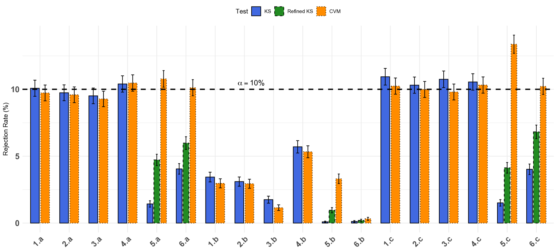
Figure 1: Rejection rates across models and cases: $n=1,000$, $\alpha=10\%$, $MC=10,000$.

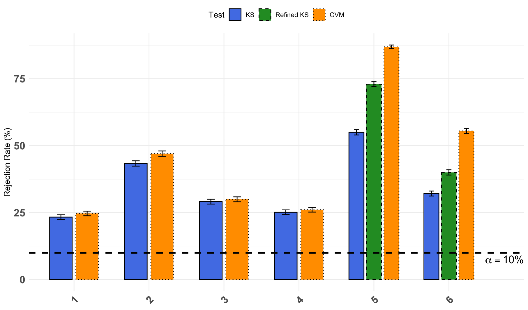
Figure 2: Rejection rates under the alternative for case d: $n=1,000$, $\alpha=10\%$, $MC=10,000$.

We report results for the case where the sample size equals $n=1,000$ and the nominal significance level is set to $\alpha=10\%$, performing $10,000$ Monte Carlo simulations to test the null hypothesis in (1). To implement the test $\phi(\cdot)$ in (11), we select the values of the tuning parameters $(q_{y},q_{x})$ using the data-dependent rules specified in (18) and (19). In addition to the KS test statistic in (7), we also provide results using the CvM test statistic in (12) for comparison. For Designs 5 and 6, where both variables are discrete, we also report the results using the refined test described in (22). For brevity, we computed the refined test only for the KS test statistic, but in principle, it could also be applied to the CvM test statistic.

Rejection probabilities $(\%)$ under $H_{0}$
Design	1				2				3
	a	b	c		a	b	c		a	b	c
$q_{y}^{*}$	79.54	78.63	34.84		79.51	79.53	34.85		45.48	44.04	20.05
$q_{x}^{*}$	79.52	79.52	34.86		79.72	89.57	34.92		45.49	45.48	20.05
Design	4				5				6
	a	b	c		a	b	c		a	b	c
$q_{y}^{*}$	83.43	83.45	36.56		96.74	102.1	44.66		59.65	60.46	26.2
$q_{x}^{*}$	83.46	83.43	36.55		96.75	96.78	42.34		59.64	59.61	26.2

Table 2: Mean values of $q_{y}^{*}$ and $q_{x}^{*}$ across simulations: $n=1,000$, $\alpha=10\%$, $MC=10,000$.

Figure 1 presents the rejection probabilities under the null hypothesis for cases (a) to (c) in each design, while Table 2 reports the mean values of $q_{y}^{*}$ and $q_{x}^{*}$ across simulations. When the data-generating process satisfies condition (1) with equality and the data are continuously distributed (case (a) in Designs 1–4), the rejection probabilities closely align with the nominal significance level. When the null hypothesis holds with strict inequality (case (b) in all designs), rejection probabilities fall below $\alpha$, consistent with our critical value serving as a valid upper bound for the true quantile. Designs 5 and 6 further demonstrate that the critical value $c_{\alpha}(q,q_{y})$ in (10) remains a valid upper bound even when the data are discrete. These designs also illustrate that the refined critical value $c^{\rm r}_{\alpha}(q,q_{y})$ in (21) offers a more accurate approximation of the true quantile of the KS test statistic, though it may still be somewhat conservative. Additionally, we observe that the CvM test statistic appears to be particularly powerful when the data are discrete, although it also exhibits over-rejection under the null hypothesis in Design 5c. These observations are not formally established by the theoretical results in this paper.

Figure 2 presents the rejection probabilities under the alternative hypothesis for all designs. The results demonstrate that the test exhibits non-trivial power across designs, that the refined critical value $c^{\rm r}_{\alpha}(q,q_{y})$ in (21) enhances power in discrete cases, and that the CvM test statistic appears to offer power advantages over the KS test statistic when the data are discretely distributed.

7 Concluding remarks

This paper introduces a novel test for conditional stochastic dominance (CSD) at target points, offering a flexible, nonparametric approach that avoids kernel smoothing while ensuring computational efficiency. By leveraging induced order statistics, our method constructs empirical cdfs using observations closest to the target conditioning point. We establish the asymptotic properties of our test, demonstrating its validity under weak regularity conditions, and derive a critical value that eliminates the need for resampling techniques such as the bootstrap. Additionally, we extend our framework to handle discrete data, proposing a refined critical value that enhances the power of the test with minimal additional information. Monte Carlo simulations align with our theoretical results and suggest that our test performs well in finite samples, making our test readily applicable to empirical research in economics, finance, and public policy.

An important feature of our test is its simplicity. Once the key tuning parameters are computed, the test only requires a standard test statistic with a deterministic critical value, without the need for kernels, local polynomials, bias correction, or bandwidth selection. Furthermore, our test admits a clear interpretation in the limit experiment, which allows us to connect it with classical analytical critical values and permutation-based tests. In this sense, our findings contribute to the broader literature on stochastic dominance testing by refining conditional inference methods and establishing new links between permutation-based and rank-based approaches. One open question we did not address in this paper concerns the validity of permutation-based tests for the hypothesis of stochastic dominance when both random variables, $Y$ and $X$, are discrete. Despite several attempts to formalize this result, we were unable to prove or disprove it. Extensive Monte Carlo simulations (not reported here) suggest that the test may be valid, and this is an area we plan to explore further.

Appendix A Proof of The Main Results

A.1 Proof of Theorem 4.1

This result is a special case of Theorem B.1 with $L=1$.

A.2 Proof of Theorem 4.2

By Theorem 4.1,

$$S_{n}\overset{d}{\to}S=(S_{1},\cdots,S_{q})$$

where the elements of $S$ are independent, and $S_{j}\sim F_{Y}(\cdot|z_{0})$ for $j=1,\cdots,q_{y}$ and $S_{j}\sim F_{X}(\cdot|z_{0})$ for $j=q_{y}+1,\cdots,q$. By the almost-sure representation theorem, we have a sequence of random vectors $\{\tilde{S}_{n}:1\leq i\leq\infty\}$ and a random vector $\tilde{S}$ defined on a common probability space $(\Omega,\mathcal{A},\tilde{P})$ such that

$$\tilde{S}_{n}\overset{d}{=}S_{n},~\tilde{S}\overset{d}{=}S,\text{ and }\tilde{S}_{n}\overset{a.s.}{\to}\tilde{S}~.$$

Let $R(s)$ denote the rank of $s$, which maps $s$ to a permutation of $\{1,2,\dots,q\}$. Define the event that the rank of the two vectors coincide as follows,

$$F_{n}=\{R(\tilde{S}_{n})=R(\tilde{S})\}~.$$

To reach the conclusion, it suffices to show that

$$\tilde{P}\{F_{n}\}\to 1~.$$ (A-1)

To see this, consider the following argument,

$$E_{P}[\phi(S_{n})] \overset{(1)}{=}E_{\tilde{P}}[\phi(\tilde{S}_{n})]\overset{(2)}{=}E_{\tilde{P}}[\phi(\tilde{S})I(F_{n})+\phi(\tilde{S}_{n})I(F_{n}^{c})]\overset{(3)}{\to}E_{\tilde{P}}[\phi(\tilde{S})]~,$$

where (1) holds by $\tilde{S}_{n}\overset{d}{=}S_{n}$, (2) by the fact that $T$ is invariant to rank-preserving transformations, and (3) by (A-1) and $\phi(\cdot)\in\{0,1\}$.

We devote the remainder of the proof to establishing (A-1). Define $\mathcal{D}=\mathcal{D}_{X}(z_{0})\cup\mathcal{D}_{Y}(z_{0})$, where $\mathcal{D}_{X}(z_{0})$ and $\mathcal{D}_{Y}(z_{0})$ denote the sets of discontinuity points as specified in Assumption 4.3. For any $\varepsilon>0$, let

$$E_{1}(\varepsilon) :=\big{\{}\{|\tilde{S}_{i}-\tilde{S}_{j}|>\varepsilon\}\cup\{\tilde{S}_{i}=\tilde{S}_{j}\in\mathcal{D}\}:i\neq j=1,\dots,q\big{\}},$$

$$E_{n,2}(\varepsilon) :=\big{\{}|\tilde{S}_{n,k}-\tilde{S}_{k}|<\varepsilon/2:k=1,\dots,q\big{\}},$$

$$E_{n,3} :=\big{\{}\{\tilde{S}_{k}\in\mathcal{D}\}\subseteq\{\tilde{S}_{k}=\tilde{S}_{n,k}\}:k=1,\dots,q\big{\}}~.$$

Observe that

$$E_{1}(\varepsilon)\cap E_{n,2}(\varepsilon)\cap E_{n,3}\subseteq F_{n}.$$ (A-2)

To establish this, consider the following argument. For any $i,j=1,\dots,q$, there are three possible cases: (i) $\tilde{S}_{i}<\tilde{S}_{j}$, (ii) $\tilde{S}_{i}>\tilde{S}_{j}$, or (iii) $\tilde{S}_{i}=\tilde{S}_{j}$. First, consider case (i), where $\tilde{S}_{i}<\tilde{S}_{j}$. Under $E_{1}(\varepsilon)$, this implies $\tilde{S}_{i}<\tilde{S}_{j}-\varepsilon$. Under $E_{n,2}(\varepsilon)$, we have $\tilde{S}_{n,i}-\varepsilon/2<\tilde{S}_{i}$ and $\tilde{S}_{j}<\tilde{S}_{n,j}+\varepsilon/2$. Combining these inequalities yields $\tilde{S}_{n,i}<\tilde{S}_{n,j}$, as required. Case (ii) follows identically by reversing the roles of $i$ and $j$. Finally, consider case (iii), where $\tilde{S}_{i}=\tilde{S}_{j}$. Under $E_{1}(\varepsilon)$, this implies $\tilde{S}_{i}=\tilde{S}_{j}\in\mathcal{D}$. By $E_{n,3}$, it follows that $\tilde{S}_{n,i}=\tilde{S}_{n,j}\in\mathcal{D}$. Since this argument holds for all $i,j=1,\dots,q$, we conclude that $F_{n}$ follows, as desired.

By (A-2), (A-1) follows that there exits $\varepsilon>0$ such that

$$\tilde{P}\{E_{1}(\varepsilon)\cap E_{n,2}(\varepsilon)\cap E_{n,3}\}\to 1.$$ (A-3)

For arbitrary $\delta>0$, (A-3) follows from finding $\varepsilon=\varepsilon(\delta)>0$ and $N(\delta)$ such that $\tilde{P}\{E_{1}(\varepsilon)\cap E_{n,2}(\varepsilon)\cap E_{n,3}\}\geq 1-\delta$ for all $n\geq N(\delta)$. Let $\varepsilon_{1}=\inf\{\|\tilde{d}-d\|/2:d<\tilde{d}\in\mathcal{D}\}>0$. By Lemma B.2, $\exists\varepsilon_{2}>0$ such that, for $i\not=j=1,\ldots,q$,

$$\tilde{P}\{\{|{\tilde{S}}_{i}-{\tilde{S}}_{j}|<\varepsilon_{2}\}\cap\{{\tilde{S}}_{i},{\tilde{S}}_{j}\in\mathcal{D}^{c}\}\} <\delta/(9q(q-1))~,$$

$$\tilde{P}\{\cup_{d\in\mathcal{D}}\{|{\tilde{S}}_{i}-{d}|<\varepsilon_{2}\}\cap\{{\tilde{S}}_{i}\in\mathcal{D}^{c}\mathcal{\}}\} <\delta/(9q(q-1))~.$$

Finally, set $\varepsilon=\min\{\varepsilon_{1},\varepsilon_{2}\}>0$ for the remainder of the proof. By elementary arguments, it suffices to show that: (i) $\tilde{P}\{E_{1}(\varepsilon)^{c}\}\leq\delta/3$, (ii) $\exists N_{2}(\delta)\in\mathbf{N}$ s.t. $\tilde{P}\{E_{n,2}(\varepsilon)^{c}\}\leq\delta/3$ for all $n\geq N_{2}(\delta)$, and (iii) $\exists N_{3}(\delta)\in\mathbf{N}$ s.t. $\tilde{P}\{E_{n,3}(\varepsilon)^{c}\}\leq\delta/3$ for all $n\geq N_{3}(\delta)$. We divide the rest of the proof into three results.

First, we show that $\tilde{P}\{E_{1}(\varepsilon)^{c}\}\leq\delta/3$. To this end, pick $i\not=j=1,\ldots,q$ arbitrarily. Note that

$$\tilde{P}\{\{|{\tilde{S}}_{i}-{\tilde{S}}_{j}|<\varepsilon\}\cap\{{\tilde{S}}_{i}={\tilde{S}}_{j}\in\mathcal{D}\}^{c}\}\stackrel{{\scriptstyle(1)}}{{\leq}}\delta/(3q(q-1))~,$$

where (1) holds by $i\not=j=1,\ldots,q$, ${\tilde{S}}_{i}$ and ${\tilde{S}}_{j}$ being identically distributed, and $\varepsilon=\min\{\varepsilon_{1},\varepsilon_{2}\}$. From here, we conclude that

$$\tilde{P}\{E_{1}(\varepsilon)^{c}\}\leq\sum_{i\not=j}\tilde{P}\{\{|{\tilde{S}}_{i}-{\tilde{S}}_{j}|<\varepsilon\}\cap\{{\tilde{S}}_{i}={\tilde{S}}_{j}\in\mathcal{D}\}^{c}\}\leq\delta/3~,$$

as desired. Second, we show that $\exists N_{2}(\delta)\in\mathbf{N}$ such that $\tilde{P}\{E_{n,2}(\varepsilon)^{c}\}\leq\delta/3$ for all $n\geq N_{2}(\delta)$. To see this, note that

$$\tilde{P}\{E_{n,2}(\varepsilon)^{c}\}\leq\sum_{k=1}^{q}P\{|\tilde{S}_{n,k}-\tilde{S}_{k}|>\varepsilon/2\}~.$$ (A-4)

By $\tilde{S}_{n}\overset{a.s.}{\to}\tilde{S}$, $\exists N_{2}(\delta)$ such that the right-hand side is less than $\delta/3$, as desired. Finally, we show that $\exists N_{3}(\delta)\in\mathbf{N}$ such that $\tilde{P}\{E_{n,3}(\varepsilon)^{c}\}\leq\delta/3$ for all $n\geq N_{3}(\delta)$. To see this, note that

$$\tilde{P}\{E_{n,3}(\varepsilon)^{c}\} =\tilde{P}\{\exists k=1,\ldots,q:\{\{\tilde{S}_{k}\in\mathcal{D}\}\subseteq\{\tilde{S}_{k}=\tilde{S}_{n,k}\}\}^{c}\}$$

$$\leq\sum_{k=1}^{q}\tilde{P}\{\{\tilde{S}_{k}\in\mathcal{D}\}\cap\{\tilde{S}_{k}\not=\tilde{S}_{n,k}\}\}~.$$

By Lemma B.1, $\exists N_{3}(\delta)$ such that the right-hand side is less than $\delta/3$, as desired. This completes the proof of (A-1) and the theorem.

A.3 Proof of Lemma 5.1

Note that

$$E_{P^{\ast}}[\phi(S)]~\overset{(1)}{\leq}~\sup_{P\in\mathbf{P}_{0}}E_{P}[\phi(S)]~\overset{(2)}{\leq}~\bar{\alpha},$$

where (1) holds by $P^{\ast}\in\mathbf{P}_{0}$ and (2) by Theorem B.2. To complete the proof, it suffices to show that $E_{P^{\ast}}[\phi(S)]=\bar{\alpha}$. To this end, consider the following argument:

$$E_{P^{\ast}}[\phi(S)] ~\overset{(1)}{=}~P^{*}\left\{\sup_{t\in\mathbf{R}}\left(\frac{1}{q_{y}}\sum_{j=1}^{q_{y}}I\{S_{j}\leq t\}-\frac{1}{q_{x}}\sum_{j=q_{y}+1}^{q}I\{S_{j}\leq t\}\right)>c_{\alpha}(q_{y},q)\right\}$$

$$~\overset{(2)}{=}~P^{*}\left\{\sup_{t\in\mathbf{R}}\left(\frac{1}{q_{y}}\sum_{j=1}^{q_{y}}I\{U_{j}\leq F(t)\}-\frac{1}{q_{x}}\sum_{j=q_{y}+1}^{q}\{U_{j}\leq F(t)\}\right)>c_{\alpha}(q_{y},q)\right\}$$

$$~\overset{(3)}{=}~P^{*}\left\{\sup_{u\in(0,1)}\left(\frac{1}{q_{y}}\sum_{j=1}^{q_{y}}I\{U_{j}\leq u\}-\frac{1}{q_{x}}\sum_{j=q_{y}+1}^{q}I\{U_{j}\leq u\}\right)>c_{\alpha}(q_{y},q)\right\}$$

$$~\overset{(4)}{=}~\bar{\alpha}~,$$ (A-5)

where (1) holds by (7), (2) holds by Pollard (2002, Eq. 36) and the same arguments used in the proof of Theorem B.2, (3) follows from the continuity of $F$ guaranteeing that

$$\sup_{t\in\mathbf{R}}\Delta\left(F(t)\right)=\sup_{u\in(0,1)}\Delta(u)$$

for $\Delta(u):=\frac{1}{q_{y}}\sum_{j=1}^{q_{y}}I\{U_{j}\leq u\}-\frac{1}{q_{x}}\sum_{j=q_{y}+1}^{q}I\{U_{j}\leq u\}$ as defined in (9), and (4) by definition of $\bar{\alpha}$ in (17).

A.4 Proof of Lemma 5.2

Let $Q:=\{Q_{1},\dots,Q_{q}\}=\{1,2,\dots,q\}$ and denote by $Q^{\pi}:=\{Q_{\pi(1)},Q_{\pi(2)}\dots,Q_{\pi(q)}\}$ the permutation $\pi=(\pi(1),\pi(2),...,\pi\left(q\right))$ of $Q$. Let $R(s)$ denote the rank of $s$, which maps $s$ to a permutation of $Q$. Since the KS statistic $T(\cdot)$ in (7) is a rank statistic, it follows that for any $s$

$$T(s)~=~T^{\ast}(R(s))~,$$ (A-6)

where $T^{\ast}$ is a known function; see Hajek et al. (1999, page 99). That is, the KS test statistic depends on $S$ only through $R(S)$. Define

$$c_{\alpha}^{\mathrm{p}}~:=~\inf_{x\in\mathbf{R}}\left\{\frac{1}{\left|\mathbf{G}\right|}\sum_{\pi\in\mathbf{G}}I\left\{T(Q^{\pi})\leq x\right\}\geq 1-\alpha\right\}~.$$ (A-7)

We divide the rest of the argument into four steps.

Step 1. For any $s\in\mathbf{R}^{q}$ with $s_{i}\not=s_{j}$ for $i\not=j$, and $c_{\alpha}^{\mathrm{p}}(s)$ as in (25),

$$c_{\alpha}^{\mathrm{p}}(s)~=~c_{\alpha}^{\mathrm{p}}~.$$

To establish this, consider the following derivation,

$$c_{\alpha}^{\mathrm{p}}(s) ~=~\inf_{x\in\mathbf{R}}\left\{\frac{1}{\left|\mathbf{G}\right|}\sum_{\pi\in\mathbf{G}}I\left\{T(s^{\pi})\leq x\right\}\geq 1-\alpha\right\}$$

$$~\overset{(1)}{=}~\inf_{x\in\mathbf{R}}\left\{\frac{1}{\left|\mathbf{G}\right|}\sum_{\pi\in\mathbf{G}}I\left\{T^{\ast}(R(s^{\pi}))\leq x\right\}\geq 1-\alpha\right\}$$

$$~\overset{(2)}{=}~\inf_{x\in\mathbf{R}}\left\{\frac{1}{\left|\mathbf{G}\right|}\sum_{\pi\in\mathbf{G}}I\left\{T^{\ast}((Q^{\bar{\pi}})^{\pi})\leq x\right\}\geq 1-\alpha\right\}$$

$$~\overset{(3)}{=}~\inf_{x\in\mathbf{R}}\left\{\frac{1}{\left|\mathbf{G}\right|}\sum_{{\pi}\in\mathbf{G}}I\left\{T^{\ast}(Q^{{\pi}})\leq x\right\}\geq 1-\alpha\right\}~\overset{(4)}{=}~c_{\alpha}^{\mathrm{p}}~.$$ (A-8)

Here, (1) follows by (A-6), (2) follows since $s_{i}\not=s_{j}$ for $i\not=j$ implies that $R(s^{\pi})=(R(s))^{\pi}$ and $R(s)=Q^{\bar{\pi}(s)}$ for some $\bar{\pi}\left(s\right)\in\mathbf{G}$, (3) by $\mathbf{G}=\tilde{\mathbf{G}}:=\{\pi\circ\bar{\pi}(s):\pi\in\mathbf{G}\}$, which follows from the fact that $\mathbf{G}$ is a group, and (4) by (A-7).

Step 2. $c_{\alpha}^{\mathrm{p}}=c_{\alpha}\left(q_{y},q\right)$, where $c_{\alpha}\left(q_{y},q\right)$ is defined in (10).

Let $\{U_{i}:1\leq i\leq q\}$ be i.i.d. with $U_{i}\sim U\left(0,1\right)$ and let $\hat{\pi}$ be a uniformly chosen permutation from $\mathbf{G}$, independent of $U$. Note that $c_{\alpha}\left(q_{y},q\right)$ is the $\left(1-\alpha\right)$-quantile of $T(U)$ and, by (A-7), $c_{\alpha}^{\mathrm{p}}$ is the $\left(1-\alpha\right)$-quantile of the cdf $\frac{1}{\left|\mathbf{G}\right|}\sum_{\pi\in\mathbf{G}}I\left\{T^{\ast}(Q^{\pi})\leq x\right\}$. The desired result then follows from noting that $\frac{1}{\left|\mathbf{G}\right|}\sum_{\pi\in\mathbf{G}}I\left\{T^{\ast}(Q^{\pi})\leq x\right\}$ is the cdf of $T(U)$, as we show next.

Let $E:=\left\{U_{i}\not=U_{j}\text{ for }i\not=j\right\}$. For any $x\in\mathbf{R}$, our desired result follows from this derivation:

$$P\left\{T(U)\leq x\right\} ~\overset{(1)}{=}~P\{T(U^{\hat{\pi}})\leq x\}$$

$$~\overset{(2)}{=}~P\left\{\left\{T(U^{\hat{\pi}})\leq x\right\}\cap E\right\}$$

$$~\overset{(3)}{=}~\int_{s\in E}\frac{1}{\left|\mathbf{G}\right|}\sum_{\pi\in\mathbf{G}}I\left\{T(u^{\pi})\leq x\right\}dP_{U}^{\ast}(u)$$

$$~\overset{(4)}{=}~\int_{u\in E}\frac{1}{\left|\mathbf{G}\right|}\sum_{\pi\in\mathbf{G}}I\left\{T^{\ast}(Q^{\pi})\leq x\right\}dP_{U}^{\ast}(u)$$

$$~\overset{(5)}{=}~\frac{1}{\left|\mathbf{G}\right|}\sum_{\pi\in\mathbf{G}}I\left\{T^{\ast}(Q^{\pi})\leq x\right\}~.$$

Here, (1) holds by $U\overset{d}{=}U^{\hat{\pi}}$, (2) and (5) by $P\{E\}=1$, (3) by $\hat{\pi}\perp U$ and $\hat{\pi}$ uniformly chosen in $\mathbf{G}$, and (4) by repeating the arguments used to derive (A-8).

Step 3. By Step 1, $\{S_{i}\not=S_{j}$ for $i\not=j\}\subseteq\left\{c_{\alpha}^{\mathrm{p}}(S)=c_{\alpha}^{\mathrm{p}}\right\}$, and so $P\left\{c_{\alpha}^{\mathrm{p}}(S)=c_{\alpha}^{\mathrm{p}}\right\}=1$ holds by our assumption. By Step 2, $c_{\alpha}^{\mathrm{p}}=c_{\alpha}\left(q_{y},q\right)$. The desired result follows from combining these points.

Step 4. To show the last statement, consider $S=\{1:1\leq j\leq q\}$. Then, $T(S^{\pi})=T(S)=0$ for all $\pi\in\mathbf{G}$, and so $c_{\alpha}^{\mathrm{p}}(S)=0$. On the other hand, Step 2 implies $c_{\alpha}^{\mathrm{p}}=c_{\alpha}\left(q_{y},q\right)$, which are positive for typical values of $\left(q_{y},q,\alpha\right)$. For example, $q_{y}=1$, $q=2$, and $\alpha=0.1$ yield $c_{\alpha}^{\mathrm{p}}=c_{\alpha}\left(q_{y},q\right)=0.5.$

Appendix B Auxiliary Results

For any $\varepsilon>0$, we use $o_{\varepsilon}(1)$ to denote an expression that converges to zero as $\varepsilon\to 0$. Analogously, for any $n\in\mathbf{N}$, we use $o_{n}(1)$ to denote an expression that converges to zero as $n\to\infty$.

B.1 Auxiliary Theorems

Theorem B.1.

Let Assumptions 4.1 and 4.2 hold with $\mathcal{Z}=\{z_{1},z_{2},\dots,z_{L}\}$, and let $S^{\ell}_{n}$ be defined as in (28). Then,

$$({S_{n}^{1}}^{\prime},\ldots,{S_{n}^{L}}^{\prime})\overset{d}{\rightarrow}({S^{1}}^{\prime},\ldots,{S^{L}}^{\prime})~,$$ (B-9)

where, for any $(s_{1}^{\ell},\dots,s_{q_{y}^{\ell}}^{\ell},s_{q_{y}^{\ell}+1}^{\ell},\dots,s_{q^{\ell}}^{\ell})\in\mathbf{R}^{q^{\ell}}$ for each $\ell=1,\dots,L$ with $q^{\ell}=q_{y}^{\ell}+q_{x}^{\ell}$, $({S^{1}}^{\prime},\ldots,{S^{L}}^{\prime})$ has the following distribution:

$$P\left\{\bigcap_{\ell=1}^{L}\bigcap_{i=1}^{q^{\ell}}\left\{S_{i}^{\ell}\leq s_{i}^{\ell}\right\}\right\}~=~\prod_{\ell=1}^{L}\prod_{i=1}^{q_{y}^{\ell}}F_{Y}(s_{i}^{\ell}|z_{\ell})\prod_{j=1}^{q_{x}^{\ell}}F_{X}(s_{j+q_{y}^{\ell}}^{\ell}|z_{\ell})~,$$

Proof.

For each $\ell=1,\dots,L$, let $M_{y}^{\ell}$ denote the subset of the indices $i=1,\dots,n_{y}$ corresponding to the $q_{y}^{\ell}$ first $g$-order statistics $(Z_{\ell,(1)},\dots,Z_{\ell,(q_{y}^{\ell})})$, and let $M_{x}^{\ell}$ denote the subset of the indices $j=1,\dots,n_{x}$ corresponding to the $q_{x}^{\ell}$ first $g$-order statistics $(Z_{\ell,(1)},\dots,Z_{\ell,(q_{x}^{\ell})})$. Let $E_{n}$ denote the following event:

$$E_{n}~=E_{n_{y},y}\cap E_{n_{x},x}\quad\text{ where }\quad E_{n_{y},y}:=\left\{\bigcap_{\ell=1}^{L}M_{y}^{\ell}=\emptyset\right\}\quad\text{and}\quad E_{n_{x},x}:=\left\{\bigcap_{\ell=1}^{L}M_{x}^{\ell}=\emptyset\right\}~.$$

In words, $E_{n}$ means that the subsets of the data used in each of the $L$ tests have no observations in common. We begin by showing that

$$P\{E_{n}\}\rightarrow 1~.$$ (B-10)

Since the two sample are independent, $P\{E_{n}\}=P\{E_{n_{y},y}\}P\{E_{n_{x},x}\}$ and so we only prove $P\{E_{n_{y},y}\}\to 1$ as the other case is analogous.

Let $\varepsilon:=\frac{1}{2}\min\left\{\left|z_{\ell}-z_{\ell^{\prime}}\right|:\ell\not=\ell^{\prime},~\ell,\ell^{\prime}=1,\ldots,L\right\}>0$. For each $\ell=1,\ldots,L$, let $B_{\ell,y}=\sum_{i=1}^{n_{y}}I\{|Z_{i}-z_{\ell}|\leq\varepsilon\}$, and note that

$$\bigcap_{\ell=1}^{L}\left\{B_{\ell,y}\geq q^{\ell}_{y}\right\}~\subseteq~E_{n}~.$$

From here, we have that (B-10) follows if we show that

$$P\{B_{\ell,y}<q^{\ell}_{y}\}\rightarrow 0\text{ for all }\ell=1,\ldots,L~.$$ (B-11)

By Assumption 4.1 and $\max_{\ell=1,\ldots,L}q^{\ell}$ being bounded, $\exists N(\varepsilon)$ s.t. for all $n_{y}\geq N\left(\varepsilon\right)$,

$$0<\frac{1}{2}P\{|Z_{i}-z_{\ell}|\leq\varepsilon\}\leq P\{|Z_{i}-z_{\ell}|\leq\varepsilon\}-\max_{\ell=1,\ldots,L}\frac{q^{\ell}_{y}}{n_{y}}~.$$ (B-12)

Then, for all $n_{y}\geq N(\varepsilon)$, we have

$$P\{B_{\ell,y}<q^{\ell}_{y}\} =P\left\{{B_{\ell,y}}/{n_{y}}-P\{|Z_{i}-z_{\ell}|\leq\varepsilon\}<{q^{\ell}_{y}}/{n_{y}}-P\{|Z_{i}-z_{\ell}|\leq\varepsilon\}\right\}$$

$$\overset{(1)}{\geq}P\{|{B_{\ell,y}}/{n_{y}}-P\{|Z_{i}-z_{\ell}|\leq\varepsilon\}|>\frac{1}{2}P\{|Z_{i}-z_{\ell}|\leq\varepsilon\}\}\overset{(2)}{\rightarrow}0~,$$

as desired, where (1) holds by (B-12) and (2) holds by the LLN as $n_{y}\to\infty$, as $B_{\ell,y}=\sum_{i=1}^{n_{y}}I\{|Z_{i}-z_{\ell}|\leq\varepsilon\}\sim Bi(n_{y},P\{|Z_{i}-z_{\ell}|\leq\varepsilon\})$.

We are now ready to prove the desired result. For any $(s_{1}^{\ell},\dots,s_{q_{y}^{\ell}}^{\ell},s_{q_{y}^{\ell}+1}^{\ell},\dots,s_{q^{\ell}}^{\ell})\in\mathbf{R}^{q^{\ell}}$ for each $\ell=1,\dots,L$ with $q^{\ell}=q_{y}^{\ell}+q_{x}^{\ell}$, we have

$$P\left\{\cap_{\ell=1}^{L}\right. \left.\cap_{i=1}^{q^{\ell}}\left\{S_{n,i}^{\ell}\leq s_{i}^{\ell}\right\}\right\}$$

$$\overset{(1)}{=}E\left[\left.P\left\{\bigcap_{\ell=1}^{L}\left\{\bigcap_{i=1}^{q_{y}^{\ell}}\left\{Y_{n,\left[i\right]}^{\ell}\leq s_{i}^{\ell}\right\}\bigcap\left\{\bigcap_{j=1}^{q_{x}^{\ell}}\left\{X_{n,\left[j\right]}^{\ell}\leq s_{j+q_{y}^{\ell}}^{\ell}\right\}\right\}\right\}\right|\mathcal{A}\right\}\right]$$

$$\overset{(2)}{=}E\left[\prod_{\ell=1}^{L}\left.P\left\{\left\{\bigcap_{i=1}^{q_{y}^{\ell}}\left\{Y_{n,\left[i\right]}^{\ell}\leq s_{i}^{\ell}\right\}\bigcap\left\{\bigcap_{j=1}^{q_{x}^{\ell}}\left\{X_{n,\left[j\right]}^{\ell}\leq s_{j+q_{y}^{\ell}}^{\ell}\right\}\right\}\right\}\right|\mathcal{A}\right\}I\{E_{n}\}\right]+o_{n}\left(1\right)$$

$$\overset{(3)}{=}E\left[\prod_{\ell=1}^{L}\left.P\left\{\left\{\bigcap_{i=1}^{q_{y}^{\ell}}\left\{Y_{n,\left[i\right]}^{\ell}\leq s_{i}^{\ell}\right\}\bigcap\left\{\bigcap_{j=1}^{q_{x}^{\ell}}\left\{X_{n,\left[j\right]}^{\ell}\leq s_{j+q_{y}^{\ell}}^{\ell}\right\}\right\}\right\}\right|\mathcal{A}\right\}\right]+o_{n}\left(1\right)$$

$$\overset{(4)}{=}E\left[\prod_{\ell=1}^{L}\prod_{i=1}^{q_{y}^{\ell}}F_{Y}(s_{i}^{\ell}|Z_{n_{y},\left(i\right)}^{\ell})\prod_{j=1}^{q_{x}^{\ell}}F_{X}(s_{j+q_{y}^{\ell}}^{\ell}|Z_{n_{x},\left(j\right)}^{\ell})\right],$$ (B-13)

where (1) holds by the LIE with $\mathcal{A}$ equal to the sigma-algebra generated by the $Z$ observations from both samples, (2) by (B-10) and the fact $E_{n}$ implies that the subsets of the data used in each of the $L$ tests have no observations in common, so they are independent conditional on $\mathcal{A}$, (3) by (B-10), and (4) by repeating the arguments in the proof of Theorem 4.1.

Next, we show that

$$Z_{n_{y},\left(i\right)}^{\ell}\overset{p}{\rightarrow}z_{\ell}~\text{ for all }~i=1,\dots,q_{y}\text{ and }~\ell=1,\ldots,L~,$$ (B-14)

$$Z_{n_{x},\left(j\right)}^{\ell}\overset{p}{\rightarrow}z_{\ell}~\text{ for all }~j=1,\dots,q_{x}\text{ and }~\ell=1,\ldots,L~.$$ (B-15)

We only show (B-14), as (B-15) can be shown analogously. To this end, fix $\ell=1,\ldots,L$ arbitrarily. We prove the result by complete induction on $i=1,\dots,q_{y}$. Take $i=1$ and fix $\epsilon>0$ arbitrarily. Then,

$$P\{|Z_{n_{y},(1)}^{\ell}-z_{\ell}|<\varepsilon\} =P\{\text{at least }1\text{ of }\{Z_{i}:1\leq i\leq n_{y}\}\text{ is s.t }\{|Z_{i}-z_{\ell}|<\varepsilon\}\}$$

$$\overset{(1)}{=}\sum_{u=1}^{n_{y}}\binom{n_{y}}{u}P\{|Z-z_{\ell}|<\varepsilon\}^{u}[1-P\{|Z-z_{\ell}|<\varepsilon\}]^{n_{y}-u}$$

$$\overset{(2)}{=}1-P\{|Z-z_{\ell}|\geq\varepsilon\}^{n_{y}}\overset{(3)}{\rightarrow}1~,$$ (B-16)

as desired, where (1) holds by the fact that $\{Z_{i}:1\leq i\leq n_{y}\}$ are identically distributed, (2) by the Binomial Theorem, and (3) by Assumption 4.1. For the inductive step, we assume $Z_{n_{y},(j)}^{\ell}-z_{\ell}=o_{p}(1)$ for $j\in\{1,\ldots,q_{y}-1\}$, and prove that $Z_{n_{y},(j+1)}^{\ell}-z_{\ell}=o_{p}(1)$. For this, consider the following derivation,

$$P\{|Z_{n_{y},(j)}^{\ell}-z_{\ell}|<\varepsilon\} =P\{\text{at least }j\text{ of the }\{Z_{i}:1\leq i\leq n_{y}\}\text{ are s.t. }\{|Z_{i}-z_{\ell}|<\varepsilon\}\}$$

$$\overset{(1)}{=}\sum_{u=j}^{n_{y}}\binom{n_{y}}{u}P\{|Z-z_{\ell}|<\varepsilon\}^{u}P\{|Z-z_{\ell}|\geq\varepsilon\}^{n_{y}-u}$$

$$\overset{(2)}{=}P\{|Z_{n_{y},(j+1)}^{\ell}-z_{\ell}|<\varepsilon\}+\binom{n_{y}}{j}P\{|Z-z_{\ell}|<\varepsilon\}^{j}P\{|Z-z_{\ell}|\geq\varepsilon\}^{n_{y}-j}~,$$

where (1) holds by the fact that $\{Z_{i}:1\leq i\leq n_{y}\}$ are identically distributed and (2) by the Binomial Theorem. The desired result then follows from assumption that $Z_{n_{y},(j)}^{\ell}-z_{\ell}=o_{p}(1)$ and the following derivation

$$\binom{n_{y}}{j}P\{|Z-z_{\ell}|<\varepsilon\}^{j}[1-P\{|Z-z_{\ell}|<\varepsilon\}]^{n_{y}-j}$$

$$\leq n_{y}^{j}P\{|Z-z_{\ell}|\geq\varepsilon\}^{n_{y}-j}=\left[e^{\frac{j\ln n_{y}}{n_{y}-j}}P\{|Z-z_{\ell}|\geq\varepsilon\}\right]^{n_{y}-j}\overset{(1)}{\rightarrow}0~,$$

where (1) follows from Assumption 4.1 and noticing that $\exists N$ s.t. $e^{\frac{j\ln n_{y}}{n_{y}-j}}P\{|Z-z_{\ell}|\geq\varepsilon\}\leq P\{|Z-z_{\ell}|\geq\varepsilon\}<1$ for all $n_{y}>N$ and any $j\in\{1,\dots,q_{y}-1\}$.

By (B-13), (B-14), and Assumption 4.2, we have

$$\lim_{n\rightarrow\infty}P\left\{\bigcap_{\ell=1}^{L}\bigcap_{i=1}^{q_{\ell}}\left\{S_{n,i}^{\ell}\leq s_{i}^{\ell}\right\}\right\}~=~\prod_{\ell=1}^{L}\prod_{i=1}^{q_{y}^{\ell}}F_{Y}(s_{i}^{\ell}|z_{\ell})\prod_{j=1}^{q_{x}^{\ell}}F_{X}(s_{j+q_{y}^{\ell}}^{\ell}|z_{\ell})~.$$ (B-17)

By definition of convergence in distribution, (B-17) implies (B-9), as desired. ∎

Theorem B.2.

Let $S$ be the random variable in Theorem 4.1. Then, for any $P\in\mathbf{P}_{0}$ and $\alpha\in(0,1)$, we obtain

$$E_{P}[\phi(S)]\leq\bar{\alpha}\leq\alpha~,$$

where

$$\bar{\alpha}:=P\left\{\sup_{u\in\mathbf{(}0,1)}\left(\frac{1}{q_{y}}\sum_{j=1}^{q_{y}}I\{U_{j}\leq u\}-\frac{1}{q_{x}}\sum_{j=q_{y}+1}^{q}I\{U_{j}\leq u\}\right)>c_{\alpha}(q_{y},q)\right\}~.$$ (B-18)

Moreover, the first inequality becomes an equality under $P$ such that $F_{Y}(t|z_{0})=F_{X}(t|z_{0})$ for all $t\in\mathbf{R}$ and these are continuous functions of $t\in\mathbf{R}$.

Proof.

Recall that $S=(S_{1},\dots,S_{q_{y}},S_{q_{y}+1},\dots,S_{q})$ are independent, and such that $S_{j}\sim F_{Y}(t|z_{0})$ for all $j=1,\dots,q_{y}$ and $S_{q_{y}+j}\sim F_{X}(t|z_{0})$ for all $j=1,\dots,q_{x}$. Denote by $Q_{Y}(\cdot|z_{0})$ and $Q_{X}(\cdot|z_{0})$ the quantile functions of $F_{Y}(t|z_{0})$ and $F_{X}(t|z_{0})$. Consider the following argument:

$$E_{P}[\phi(S)] =P\left\{\max_{k\in\{1,\dots,q_{y}\}}\left(\frac{1}{q_{y}}\sum_{j=1}^{q_{y}}I\{S_{j}\leq S_{k}\}-\frac{1}{q_{x}}\sum_{j=q_{y}+1}^{q}I\{S_{j}\leq S_{k}\}\right)>c_{\alpha}(q_{y},q)\right\}$$

$$\overset{(1)}{=}P\left\{\sup_{t\in\mathbf{Y}}\left(\frac{1}{q_{y}}\sum_{j=1}^{q_{y}}I\{Q_{Y}(U_{j}|z_{0})\leq t\}-\frac{1}{q_{x}}\sum_{j=q_{y}+1}^{q}I\{Q_{X}(U_{j}|z_{0})\leq t\}\right)>c_{\alpha}(q_{y},q)\right\}$$

$$\overset{(2)}{=}P\left\{\sup_{t\in\mathbf{Y}}\left(\frac{1}{q_{y}}\sum_{j=1}^{q_{y}}I\{U_{j}\leq F_{Y}(t|z_{0})\}-\frac{1}{q_{x}}\sum_{j=q_{y}+1}^{q}I\{U_{j}\leq F_{X}(t|z_{0})\}\right)>c_{\alpha}(q_{y},q)\right\}$$

$$\overset{(3)}{\leq}P\left\{\sup_{t\in\mathbf{Y}}\left(\frac{1}{q_{y}}\sum_{j=1}^{q_{y}}I\{U_{j}\leq F_{X}(t|z_{0})\}-\frac{1}{q_{x}}\sum_{j=q_{y}+1}^{q}I\{U_{j}\leq F_{X}(t|z_{0})\}\right)>c_{\alpha}(q_{y},q)\right\}$$

$$\overset{(4)}{=}P\left\{\sup_{u\in\mathcal{U}}\left(\frac{1}{q_{y}}\sum_{j=1}^{q_{y}}I\{U_{j}\leq u\}-\frac{1}{q_{x}}\sum_{j=q_{y}+1}^{q}I\{U_{j}\leq u\}\right)>c_{\alpha}(q_{y},q)\right\}$$

$$\overset{(5)}{\leq}P\left\{\sup_{u\in\mathbf{(}0,1)}\left(\frac{1}{q_{y}}\sum_{j=1}^{q_{y}}I\{U_{j}\leq u\}-\frac{1}{q_{x}}\sum_{j=q_{y}+1}^{q}I\{U_{j}\leq u\}\right)>c_{\alpha}(q_{y},q)\right\}$$

$$\overset{(6)}{=}\bar{\alpha}~,$$

where (1) follows from the quantile transformation and the fact that replacing $\max_{k\in\{1,\dots,q_{y}\}}$ with $\sup_{t\in\mathbf{Y}}$ does not affect the magnitude of the test statistic, (2) follows from Pollard (2002, Eq. 36), (3) from $P\in\mathbf{P}_{0}$, (4) from a simple change of variables and $\mathcal{U}:=\cup_{t\in\mathbf{Y}}\{u=F_{X}(t|z_{0})\}$, (5) from $\mathcal{U}\subseteq(0,1)$, and (6) from the definition of $c_{\alpha}(q_{y},q)$ and $\bar{\alpha}$, and the fact that $\{U_{j}:j=1,\dots,q\}$ are i.i.d. distributed as $U(0,1)$.

To conclude the proof, it suffices to show that: (i) inequality (3) holds as an equality under the condition $F_{Y}(t\mid z_{0})=F_{X}(t\mid z_{0})$ for all $t\in\mathbf{R}$, and (ii) inequality (5) holds as an equality when these functions are continuous in $t$. The first claim is immediate. For the second, it follows from the fact that the continuity of the CDFs implies $\mathcal{U}=(0,1)$. By elementary properties of cdfs, $\lim_{t\to-\infty}F_{X}(t\mid z_{0})=0$ and $\lim_{t\to\infty}F_{X}(t\mid z_{0})=1$. By the intermediate value theorem, for any $u\in(0,1)$, there exists $t\in\mathbf{R}$ such that $u=F_{X}(t\mid z_{0})$, implying $u\in\mathcal{U}$, as desired. ∎

B.2 Auxiliary Lemmas

Lemma B.1.

Suppose Assumptions 4.1, 4.2, and 4.3 hold. Consider a sequence of random vectors $\{\tilde{S}_{n}:1\leq n<\infty\}$ and a random vector $\tilde{S}$ defined on a common probability space $(\Omega,\mathcal{A},\tilde{P})$ such that

$$\tilde{S}_{n}\overset{d}{=}S_{n},\quad\tilde{S}\overset{d}{=}S,\quad\text{ and }\quad\tilde{S}_{n}\overset{a.s.}{\to}\tilde{S}~.$$ (B-19)

Then, for any $j\in\{1,\dots,q\}$,

$$\tilde{P}\{\tilde{S}_{n,j}\neq\tilde{S}_{j},~\tilde{S}_{j}\in\mathcal{D}\}=o_{n}(1)~.$$

Proof.

We focus on an arbitrary $j\in\{1,\dots,q_{y}\}$. The argument for $j\in\{q_{y}+1,\dots,q\}$ follows analogously by replacing $Y$ with $X$. By Lemma B.4, it suffices to show that

$$\sup_{t\in\mathbb{R}}\big{|}F_{\tilde{S}_{n,j}}(t)-F_{\tilde{S}_{j}}(t)\big{|}=o_{n}(1)~,$$ (B-20)

where $F_{\tilde{S}_{n,j}}$ and $F_{\tilde{S}_{j}}$ denote the distribution functions of $\tilde{S}_{n,j}$ and $\tilde{S}_{j}$ in $(\Omega,\mathcal{A},\tilde{P})$.

By the proof in Theorem B.1 (with $L=1$ and $\mathcal{Z}=\{z_{0}\}$), we have $F_{S_{j}}(t)=F_{Y}(t|z_{0})$ and $F_{S_{n,j}}(t)=E[F_{Y}(t|Z_{n_{y},(j)})]$ where $Z_{n_{y},(j)}\overset{p}{\to}z_{0}$. By these and (B-19), (B-20) follows from

$$\sup_{t\in\mathbf{R}}|E[F_{Y}(t|Z_{n_{y},(j)})]-F_{Y}(t|z_{0})|=o_{n}(1)~.$$ (B-21)

For any $\varepsilon>0$,

$$E[F_{Y}(t|Z_{n_{y},(j)})] =\int_{|z-z_{0}|\leq\varepsilon}F_{Y}(t|z)dP_{Z_{n_{y},(j)}}(z)+\int_{|z-z_{0}|>\varepsilon}F_{Y}(t|z)dP_{Z_{n_{y},(j)}}(z)$$

$$\leq\int_{|z-z_{0}|\leq\varepsilon}F_{Y}(t|z)dP_{Z_{n_{y},(j)}}(z)+P(|Z_{n_{y},(j)}-z_{0}|>\varepsilon)$$

$$\overset{(1)}{=}\int_{|z-z_{0}|\leq\varepsilon}F_{Y}(t|z)dP_{Z_{n_{y},(j)}}(z)+o_{n}(1)~,$$

where (1) holds by $Z_{n_{y},(j)}\overset{p}{\to}z_{0}$. Then,

$$\sup_{t\in\mathbf{R}}|E[F_{Y}(t|Z_{n_{y},(j)})]-F_{Y}(t|z_{0})|\leq\sup_{t\in\mathbf{R}}\sup_{|z-z_{0}|\leq\varepsilon}|F_{Y}(t|z)-F_{Y}(t|z_{0})|+o_{n}(1)~.$$

Fix $\delta>0$ arbitrarily. By Assumption 4.2, $\exists\varepsilon>0$ such that $\sup_{t\in\mathbf{R}}\sup_{|z-z_{0}|\leq\varepsilon}|F_{Y}(t|z)-F_{Y}(t|z_{0})|<\delta/2$. For all large enough $n_{y}$, the right-hand side is bounded above by $\delta$. Since the choice of $\delta$ was arbitrary, (B-21) follows. ∎

Lemma B.2.

Let $V_{1}$ and $V_{2}$ be independent random variables that are discontinuous at a finite set of points $\mathcal{D}_{1}$ and $\mathcal{D}_{2}$, respectively. Then, for any $\delta>0$, $\exists\varepsilon>0$ small enough s.t.

$$P\{\cup_{d\in\mathcal{D}_{1}}\{|V_{1}-d|<\varepsilon\}\cap\{V_{1}\in\mathcal{D}_{1}^{c}\}\} <\delta~,$$

$$P\{\{|V_{1}-V_{2}|<\varepsilon\}\cap\{V_{1}\in\mathcal{D}_{1}^{c}\}\cap\{V_{2}\in\mathcal{D}_{2}^{c}\}\} <\delta~.$$

Proof.

Set $\bar{\varepsilon}:=\{\min|d-\tilde{d}|:d,\tilde{d}\in\mathcal{D}_{1}\cap d\not=\tilde{d}\}>0$. For any $\varepsilon\in(0,\bar{\varepsilon}/2),$

$$P\{\cup_{d\in\mathcal{D}_{1}}\{|V_{1}-d|<\varepsilon\}\cap\{V_{1}\in\mathcal{D}_{1}^{c}\}\} \leq\sum_{d\in\mathcal{D}_{1}}P\{\{|V_{1}-d|<\varepsilon\}\cap\{V_{1}\in\mathcal{D}_{1}^{c}\}\}$$

$$\leq_{(1)}\sum_{d\in\mathcal{D}_{1}}P\{V_{1}\in(d-\varepsilon,d)\cup(d,d+\varepsilon)\}\overset{(2)}{=}o_{\varepsilon}(1)~,$$

where (1) holds by $\varepsilon\in(0,\bar{\varepsilon}/2)$ and (2) by the fact that $(d-\varepsilon,d)\cap(d,d+\varepsilon)$ has no discontinuities in the cdf. The right-hand side is less than $\delta$ by making $\varepsilon$ arbitrarily small, as desired. Also, for any $\varepsilon\in(0,\bar{\varepsilon}/2)$,

$$P\{\{|V_{1}-V_{2}|<\varepsilon\}\cap\{V_{1}\in\mathcal{D}_{1}^{c}\}\cap\{V_{2}\in\mathcal{D}_{2}^{c}\}\}$$

$$\overset{(1)}{=}\int_{\mathcal{D}_{2}^{c}}P\{\{|V_{1}-v_{2}|<\varepsilon\}\cap\{V_{1}\in\mathcal{D}_{1}^{c}\}\}dP_{V_{2}}(v_{2})\overset{(2)}{=}o_{\varepsilon}(1)~,$$

where (1) holds by $V_{1}\perp V_{2}$, and (2) holds by Lemma B.3 and the dominated convergence theorem. The right-hand side is less than $\delta$ by making $\varepsilon$ arbitrarily small, as desired. ∎

Lemma B.3.

Consider a random variable $V$ whose cdf is discontinuous at a finite set of points $\mathcal{D}$. Then, for any $v\in\mathbf{R}$,

$$P\{\{|V-v|<\varepsilon\}\cap\{V\in\mathcal{D}^{c}\}\}=o_{\varepsilon}(1)~.$$

Proof.

Set $\bar{\varepsilon}:=\{\min|d-\tilde{d}|:d,\tilde{d}\in\mathcal{D}_{1}\cap d\not=\tilde{d}\}>0$. Fix $\varepsilon<\bar{\varepsilon}/2$. There are two possibilities: $v\in\mathcal{D}$ or $v\not\in\mathcal{D}$. First, consider $v\in\mathcal{D}$. In this case,

$$P\{|V-v|<\varepsilon\}\cap\{V\in\mathcal{D}^{c}\}\leq P\{V\in(v-\varepsilon,v)\cap(v,v+\varepsilon)\}\overset{(1)}{=}o_{\varepsilon}(1)~,$$

where (1) holds because $(d-\varepsilon,d)\cap(d,d+\varepsilon)$ has no mass points. Second, consider $v\not\in\mathcal{D}$. Then,

$$P\{\{|V-v|<\varepsilon\}\cap\{V\in\mathcal{D}^{c}\}\}\leq F_{V}(v+\varepsilon)-F_{V}(v-\varepsilon)\overset{(2)}{=}o_{\varepsilon}(1)~,$$

where (1) by the fact that $(v-\varepsilon,v+\varepsilon]$ has no mass points, so $F_{V}$ is continuous on that interval. ∎

Lemma B.4.

Let $\{V_{n}:n\geq 1\}$ be a sequence of random variables that satisfy $V_{n}\overset{p}{\to}V$, where $V$ is a random variable whose cdf is discontinuous at a finite set of points $\mathcal{D}$. Furthermore, assume $\sup_{t\in\mathbf{R}}|F_{V_{n}}(t)-F_{V}(t)|\to 0$. Then,

$$P\{\{V\in\mathcal{D}\}\cap\{V_{n}\neq V\}\}\to 0~.$$

Proof.

Fix $\delta>0$ arbitrarily. It suffices to find $N=N(\delta)$ such that $P\{V\in\mathcal{D},V_{n}\neq V\}<\delta$ for all $n>N$.

Set $\bar{\varepsilon}:=\{\min|d-\tilde{d}|:d,\tilde{d}\in\mathcal{D}\cap d\not=\tilde{d}\}>0$. For any $\varepsilon\in(0,\bar{\varepsilon}/2),$ consider the following argument.

$$P\{\{V\in\mathcal{D}\}\cap\{V_{n}\neq V\}\} =\sum_{d\in\mathcal{D}}P\{\{V=d\}\cap\{V_{n}\neq d\}\}$$

$$\overset{(1)}{=}\sum_{d\in\mathcal{D}}P\{\{V=d\}\cap\{V_{n}\neq d\}\cap\{|V_{n}-d|<\varepsilon\}\}+o_{n}(1)$$

$$\leq\sum_{d\in\mathcal{D}}P\{V_{n}\in(d-\varepsilon,d)\cap(d,d+\varepsilon)\}+o_{n}(1)$$

$$\overset{(2)}{=}\sum_{d\in\mathcal{D}}P\{V\in(d-\varepsilon,d)\cap(d,d+\varepsilon)\}+o_{n}(1)$$

$$\overset{(3)}{=}o_{\varepsilon}(1)+o_{n}(1)~,$$

where (1) holds by $V_{n}\overset{p}{\to}V$, (2) by $\sup_{t\in\mathbf{R}}|F_{V_{n}}(t)-F_{V}(t)|=o_{n}(1)$, and (3) by the fact that $(d-\varepsilon,d)\cap(d,d+\varepsilon)$ has no discontinuities in the CDF. For all large enough $n$ and small enough $\varepsilon$, the right-hand side is bounded by $\delta$, as desired. ∎

References

- Abadie (2002) Abadie, A. (2002). Bootstrap tests for distributional treatment effects in instrumental variable models. Journal of the American statistical Association, 97 284–292.
- Anderson (1996) Anderson, G. (1996). Nonparametric tests of stochastic dominance in income distributions. Econometrica: Journal of the Econometric Society 1183–1193.
- Andrews and Shi (2017) Andrews, D. W. and Shi, X. (2017). Inference based on many conditional moment inequalities. Journal of Econometrics, 196 275–287.
- Armstrong and Kolesár (2018) Armstrong, T. B. and Kolesár, M. (2018). Optimal inference in a class of regression models. Econometrica, 86 655–683.
- Barrett and Donald (2003) Barrett, G. F. and Donald, S. G. (2003). Consistent tests for stochastic dominance. Econometrica, 71 71–104.
- Becker (1957) Becker, G. S. (1957). The economics of discrimination. University of Chicago Press Economics Books.
- Bharadwaj et al. (2024) Bharadwaj, P., Deb, R. and Renou, L. (2024). Statistical discrimination and the distribution of wages. Tech. rep., National Bureau of Economic Research.
- Bhattacharya (1974) Bhattacharya, P. (1974). Convergence of sample paths of normalized sums of induced order statistics. The Annals of Statistics 1034–1039.
- Blackman (1956) Blackman, J. (1956). An extension of the kolmogorov distribution. The Annals of Mathematical Statistics 513–520.
- Bugni and Canay (2021) Bugni, F. A. and Canay, I. A. (2021). Testing continuity of a density via g-order statistics in the regression discontinuity design. Journal of Econometrics, 221 138–159.
- Bugni et al. (2018) Bugni, F. A., Canay, I. A. and Shaikh, A. M. (2018). Inference under covariate adaptive randomization. Journal of the American Statistical Association, 113 1784–1796.
- Canay and Kamat (2018) Canay, I. A. and Kamat, V. (2018). Approximate permutation tests and induced order statistics in the regression discontinuity design. The Review of Economic Studies, 85 1577–1608.
- Canay et al. (2024) Canay, I. A., Mogstad, M. and Mountjoy, J. (2024). On the use of outcome tests for detecting bias in decision making. Review of Economic Studies, 91 2135–2167.
- Canay et al. (2017) Canay, I. A., Romano, J. P. and Shaikh, A. M. (2017). Randomization tests under an approximate symmetry assumption. Econometrica, 85 1013–1030.
- Caughey et al. (2023) Caughey, D., Dafoe, A., Li, X. and Miratrix, L. (2023). Randomisation inference beyond the sharp null: bounded null hypotheses and quantiles of individual treatment effects. Journal of the Royal Statistical Society Series B: Statistical Methodology, 85 1471–1491.
- Chang et al. (2015) Chang, M., Lee, S. and Whang, Y.-J. (2015). Nonparametric tests of conditional treatment effects with an application to single-sex schooling on academic achievements. The Econometrics Journal, 18 307–346.
- Chung and Romano (2013) Chung, E. and Romano, J. P. (2013). Exact and asymptotically robust permutation tests. The Annals of Statistics, 41 484–507.
- David and Galambos (1974) David, H. and Galambos, J. (1974). The asymptotic theory of concomitants of order statistics. Journal of Applied Probability 762–770.
- Davidson and Duclos (2000) Davidson, R. and Duclos, J.-Y. (2000). Statistical inference for stochastic dominance and for the measurement of poverty and inequality. Econometrica, 68 1435–1464.
- Delgado and Escanciano (2013) Delgado, M. A. and Escanciano, J. C. (2013). Conditional stochastic dominance testing. Journal of Business & Economic Statistics, 31 16–28.
- Donald et al. (2012) Donald, S. G., Hsu, Y.-C. and Barrett, G. F. (2012). Incorporating covariates in the measurement of welfare and inequality: methods and applications. The Econometrics Journal, 15 C1–C30.
- Durbin (1973a) Durbin, J. (1973a). Distribution theory for tests based on the sample distribution function. SIAM.
- Durbin (1973b) Durbin, J. (1973b). Distribution theory for tests based on the sample distribution function. SIAM.
- Gnedenko and Koroluk (1951) Gnedenko, B. V. and Koroluk, V. S. (1951). On the maximum divergence of two empirical distributions (in russian). DAN, 80 525.
- Gnedenko and Korolyuk (1951) Gnedenko, B. V. and Korolyuk, V. S. (1951). On the maximum divergence of two empirical distributions (in russian). DAN, 80 525.
- Gonzalo and Olmo (2014) Gonzalo, J. and Olmo, J. (2014). Conditional stochastic dominance tests in dynamic settings. International Economic Review, 55 819–838.
- Hajek et al. (1999) Hajek, J., Sidak, Z. and Sen, P. K. (1999). Theory of rank tests. 2nd ed. Academic press.
- Hodges (1958) Hodges, J. (1958). The significance probability of the smirnov two-sample test. Arkiv för matematik, 3 469–486.
- Hájek and Šidák (1967) Hájek, J. and Šidák, Z. (1967). Theory of Rank Tests. Academic Press, New York.
- Kaufmann and Reiss (1992) Kaufmann, E. and Reiss, R.-D. (1992). On conditional distributions of nearest neighbors. Journal of Multivariate Analysis, 42 67–76.
- Korolyuk (1955) Korolyuk, V. S. (1955). On the discrepancy of empiric distributions for the case of two independent samples. Izv. Akad. Nauk SSSR Ser. Mat., 19 81–96.
- Lehmann and Romano (2005) Lehmann, E. and Romano, J. P. (2005). Testing Statistical Hypotheses. 3rd ed. Springer, New York.
- Lehmann (1951) Lehmann, E. L. (1951). Consistency and unbiasedness of certain nonparametric tests. The annals of mathematical statistics 165–179.
- Linton et al. (2005) Linton, O., Maasoumi, E. and Whang, Y.-J. (2005). Consistent testing for stochastic dominance under general sampling schemes. The Review of Economic Studies, 72 735–765.
- Linton et al. (2010) Linton, O., Song, K. and Whang, Y.-J. (2010). An improved bootstrap test of stochastic dominance. Journal of Econometrics, 154 186–202.
- McFadden (1989) McFadden, D. (1989). Testing for stochastic dominance. In Studies in the economics of uncertainty: In honor of Josef Hadar. Springer, 113–134.
- Pollard (2002) Pollard, D. (2002). A User’s Guide to Measure Theoretic Probability. Cambrigde University Press, New York.
- Qu and Yoon (2019) Qu, Z. and Yoon, J. (2019). Uniform inference on quantile effects under sharp regression discontinuity designs. Journal of Business & Economic Statistics, 37 625–647.
- Reiss (1989) Reiss, R.-D. (1989). Approximate distributions of order statistics: with applications to nonparametric statistics. Springer-Verlag, New York.
- Shen (2019) Shen, S. (2019). Estimation and inference of distributional partial effects: Theory and application. Journal of Business & Economic Statistics, 37 54–66.
- Shen and Zhang (2016) Shen, S. and Zhang, X. (2016). Distributional tests for regression discontinuity: Theory and empirical examples. Review of Economics and Statistics. Forthcoming.
- Smirnov (1939) Smirnov, N. V. (1939). On the estimation of the discrepancy between empirical curves of distributions for two independent samples (in russian). Bull. MGU, 2.