Non-Gaussianities as a Signature of Quantumness of Quantum Cosmology
Abstract
We show that the consistent application of the rules of quantum mechanics to cosmological systems inevitably results in the so-called multiverse states in which neither the background spacetime nor the inhomogeneous perturbation are in definite states. We study the multiverse states as perturbations to the usually employed so-called Born-Oppenheimer states that are products of a wave function of the background and a wave function of the perturbation. The obtained corrections involve integrals over virtual backgrounds that represent the effect of quantum background fluctuations on the perturbation state. They resemble loop corrections in quantum field theory. This approach demonstrates the inevitable existence of very specific non-Gaussian features in primordial fluctuations. We express the resulting non-Gaussian perturbation as a nonlinear function of the Gaussian perturbation obtained within the Born-Oppenheimer approximation, and compute its trispectrum, to show that the multiverse scenario leads to testable and distinct signatures in cosmological perturbations. Our approach applies both to inflationary and alternative cosmologies.
I Introduction
Virtually all quantum cosmological models [1, 2, 3] that are discussed in the literature assume the quantum state of the universe to be the tensor-product of wavefunctions for the background mode and the perturbation modes (see, for instance, Refs. [4, 5, 6, 7, 8, 9, 10, 11, 12, 13, 14]). We shall refer to this assumption as the Born-Oppenheimer (BO) factorization. It is important to note that this assumption is highly restrictive, as such states, called in what follows Born-Oppenheimer (BO) states, occupy a set of measure-zero in the space of all possible quantum gravity states, even though some justification can be provided from a decoherence point of view [15]. Despite the fact that such quantum states can make some observationally consistent predictions for primordial perturbations, the respective quantum cosmological models may seem overly simplistic and, to some extent, questionable. Such a viewpoint is particularly legitimate in case of the models that address the initial singularity problem.
Apart from computational simplicity, there is no inherent reason to assume that the universe should adhere to the BO factorization. On the contrary, had the quantum effects been really significant in the primordial universe, it is natural to expect that the underlying state would not respect this artificial factorization. Indeed, as our previous study [16] showed, a simple bouncing model typically evolves an initial BO state into a more generic one. The latter is an entangled state that cannot be expressed as a product state of the background and the perturbation but rather as a sum, possibly infinite, of such products. In other words, neither the background geometry nor any perturbation mode emerges from the big bang in a definite state. Therefore, the conventional splitting of cosmological spacetime into the background and the perturbation, which can be disputed at the classical level [17], turns out to be dissolved into entangled states by quantum gravity. Despite that entangled states arise from quantization of a single-universe model, we call them the multiverse states as each of them carries the potentiality of multiple cosmological scenarios. It is noteworthy that a consistent application of the rules of quantum mechanics to general relativity inevitably results in the emergence of this multiverse framework.
The idea of the multiverse is very attractive in the view of how finely-tuned our Universe appears [18]. It posits that our cosmos is just one among numerous other universes that are governed by the same fundamental laws but admit different initial conditions [19]. Although, the multiverse idea is not new, it has never been given, to the best of our knowledge, the specific form described above. In the context of inflationary models, the multiverse refers to multiple, disconnected, expanding regions, characterized by different cosmological parameters and existing within a single and well-defined spacetime, even if vast or infinite [20]. In the context of the many-world interpretation of quantum mechanics [21], the multiverse is indeed made of multiple branches of the wave function of the Universe, but the branching is usually understood as a process of splitting the worlds by means of many small variations in local degrees of freedom, and the discussions thereof do not normally involve the perturbed cosmological model studied herein. Our results are, moreover, independent of any specific interpretation of, or approach to, quantum mechanics.
Apart from the fact that the multiverse idea can help explain the fine-tuning of the initial condition, the significance of our specific multiverse model lies in the fact that it makes experimentally testable predictions. This is contrary to the common perception of the multiverse as an interesting but fundamentally untestable idea. We prove that the different branches of the multiverse state can interact, leaving a distinct imprint of this interaction in the primordial structure of the Universe. Interestingly, one of the predicted multiverse signatures, the non-Gaussianity of the primordial density fluctuations, is produced via interaction of the perturbation modes with the quantum background rather than higher-order interactions among the perturbation modes themselves. This makes our prediction distinct from and independent of any specific higher-order extension to the linear cosmological perturbation theory.
With this work, we develop the multiverse framework initiated in our previous work [16] where a coarse-grained approach to the multiverse dynamics was established. Presently, we focus on developing a perturbative approach based on the expansion of a generic state of the universe in terms of the BO states. With this new approach, as will become clearer later, we circumvent any potential stability issue, likely present in the complete multiverse dynamics. In what follows we make no assumption on the details of the underlying quantum model, which results in a broad framework that is applicable both to inflationary and alternative (e.g., big-bounce) models. The only restriction we assume is that the states must be perturbatively close to the BO states.
This new approach confirms and extends our previous result on the existence of non-Gaussianity in primordial fluctuations as a direct consequence of the entangling dynamics. Actually, it enables to pin down the shape and the amplitude of non-Gaussianity via a four-point correlation function. Thus, our result lays the foundations for experimental verification of the multiverse scenario.
The plan of this work is as follows. In Sec. II, we discuss the idea of a generic quantum state of the universe together with the Born-Oppenheimer-like restriction imposed on it in the usual approach to quantum cosmology. Sec. III introduces a useful tool which is a projection operator, and shows how it applies to the discussions of both the Born-Oppenheimer and the multiverse states. Sec. IV derives the main result of this work, which is the formula (55) for the multiverse state from a perturbation theory. Sec. V uses the result of the preceding section for computation of the four-point correlation function that is given a specific analytical form. We summarize our work in Sec. VI.
II Quantum Universe
The general framework of quantum postulates splits physical world into (a) the quantized system which is under study, and for which no “objective" properties can be assumed to exist, and (b) an external domain, or the “observer", for which unique properties of the studied system exist, and are statistically predictable with the probabilities obtainable from the quantum formalism. However, these postulates cannot be directly applied to our entire Universe that (a) is unique by definition, and (b) does not possess any “external domain", or equivalently, (b’) internally includes any potential observer.
In this work, instead of trying to solve this outstanding issue, we take an approach allowing us to use the standard Hilbert space formalism and make physical predictions in a consistent way. We explain our way of applying quantum formalism below.
II.1 Quantum Cosmological Background
We shall assume that only one time-dependent state of a cosmological background, denoted by , represents our Universe. Furthermore, we assume that the state satisfies the background Schrödinger equation at all times,
so that the quantum background evolution of our Universe corresponds to a fixed, specific state-trajectory,111We proved in Ref. [22] that coherent states exist that evolve parametrically, i.e. , under the action of . They are very good candidates to specify state-trajectories.
where is the conformal time as measured with respect to an arbitrary origin.
When a specific state-trajectory is chosen to represent our Universe, all other states, denoted as , must be seen as “virtual states" corresponding to potential configurations that the system could assume, but in fact it does not. A quantum jump from one trajectory to another is prohibited because there is no possible measurement performed by an apparatus outside our Universe, producing a non-unitary evolution of , and thereby breaking the Schrödinger equation. However, coupling the perturbation modes to the background geometry generically causes the quantum background to spread into all the other branches , with each branch in turn influencing the perturbation modes in a distinctive manner. Although the virtual background states remain physically inaccessible, their effect on the perturbation modes is potentially observable and thus, physically relevant.
In the following, we assume that the set of states (including ) resolves the identity, i.e.,
and forms a basis for the background Hilbert space .
II.2 Virtual Backgrounds
The point of view taken in this work suggests that the only observable background quantities are the expectation values of any quantum operators in the state , understood as "classical" quantities, e.g., the scale factor. Note that this implies that the usually postulated observables of ordinary quantum mechanics, that is, the eigenvalues of real operators, are in general excluded from the proposed formalism.
Instead, we can predict the expectations values of any observable as functions of time in the background state of interest . The effect of virtual states appear when, for example, we compute the expectation value of a compound observable such as , which, thanks to the resolution of the identity, is given by
| (1) |
This actually differs from , and instead, one often gets
| (2) |
where the renormalization factor can be interpreted as the effect of virtual states . It is similar (but not completely equivalent) to loop corrections in quantum field theory.
II.3 Perturbing the background
The classical Hamiltonian can be obtained from the ADM formalism by truncating it at second order of perturbations and solving both the background-level and the linearized constraints. This procedure involves the choice of some internal time, which for the purpose of this study has been conveniently set to coincide with conformal time (see our previous work [16] for more details). The validity of the truncation rests on the assumption of smallness of the perturbations to homogeneity. For a perturbed flat FLRW universe filled with a perfect fluid, we have
| (3) |
where are canonical background variables and
describes the dynamics of the are canonical perturbation variables for the Fourier modes . Note that, the perturbations being real, we have ; this relation will still hold in the quantum context below. We also assume that our perturbation model (3) represents an effective field theory and is thus only valid for a limited range of wave vectors 222Actually, in standard cosmology with slightly red power spectrum ( with ), setting is not necessary, whereas reflects the finite size of the studied spacetime region..
The truncated Hamiltonian is physically correct, i.e., consistent with the initial assumption, only if the Hamilton equations for the background deduced from are almost the same as those obtained from . Or put differently, the inevitable (for ) dynamical backreaction of the perturbation variables on the background , induced by , must always remain very weak. But in fact we see that the backreaction is induced by the change
| (4) |
Therefore, the backreaction is negligible only if , which is consistent with our assumption that the theory is meaningful only in a limited range of . Far from a singularity (), this constraint can certainly be satisfied and dynamically preserved, i.e., made valid uniformly in time. However, on the approach to the singularity, it cannot be ensured that the backreaction remains weak. Indeed, sufficiently close to the singularity, even if the linear Hamilton equations for the perturbations variables are assumed to remain valid, the background variables may no longer satisfy the zeroth-order equations of motion.
One could conclude that the perturbation framework is simply not valid close to the singularity, and that the calculations cannot be trusted in this regime. However, there exists a mathematically consistent way to keep the perturbation framework by explicitly removing the backreaction The idea is to solve the Hamilton equations in two steps:
(a) we first specify a background trajectory only by using the background-level Hamiltonian ,
(b) then we find the evolution of the perturbation variables and by using the time-dependent Hamiltonian . This is in fact the usual approach to perturbation theory at the classical level.
The quantum counterpart of the classical system involves two partial Hilbert spaces: for the background and for the perturbations. The total Hilbert space is therefore the tensor product . We have a quantum Hamiltonian acting only on for the background and a quantum perturbation Hamiltonian acting on . In order to avoid any kind of quantum backreaction from the perturbation modes on the quantum background, we need to follow a two-step procedure similar to the classical one. This leads us to the Born-Oppenheimer factorization, as we explain below.
II.4 Born-Oppenheimer factorization
Following the previous analysis of the quantum background, we first specify a trajectory-state that follows the Schrödinger equation. This corresponds to the step (a) of the classical procedure. The quantum counterpart of the step (b) is given by the solution of the following Schrödinger equation for the perturbation modes
| (5) |
with
| (6) |
where represents the operator averaged on the background state . Therefore, even though it may look as a scalar product, the quantity remains an operator, but one that acts only on the perturbation space . This procedure involves a factorized global state which we refer to as the Born-Oppenheimer state.
II.5 Beyond Born-Oppenheimer factorization
Quantum formalism introduces physical effects that have no classical counterparts such as quantum entanglement. It turns out that it is possible to go beyond the Born-Oppenheimer factorization and find the effects of entanglement while staying within a quantum counterpart of the previously described two-step procedure.
The idea is that the virtual background states, thanks to the background dynamical loops, are able to produce new effects that have no equivalent in the classical domain, but are neglected by the Born-Oppenheimer factorization. In other words, the background quantum fluctuations are able to modify the Born-Oppenheimer states. The corresponding corrections are similar to the loop corrections in quantum field theory.
Let us define the complete (time-independent) Hamiltonian as
| (7) |
and let us consider a general state , which satisfies the full Schrödinger equation:
| (8) |
The state can be interpreted as a multiverse state, as it potentially involves a superposition of different Born-Oppenheimer states. Indeed, even if the evolution starts from a factorized state at time , i.e., , at later times this state develops into a multiverse state . This is so because the action of the Hamiltonian involves mixing between different background states (i.e., is in general non-diagonal in states ). Furthermore, the multiverse state includes the quantum backreaction from the perturbation on the background, which is inevitable and may grow uncontrollably, and the assumption of its weakness could break down. This is similar to the classical situation where we directly apply the complete classical Hamiltonian of Eq. (3).
Starting from the Schrödinger equation (8), at first sight it seems impossible to respect the constraint of the weak backreaction, and the Born-Oppenheimer factorization seems to be the only way to implement this constraint at the quantum level.
But this conclusion is too rash, and in fact a generic multiverse state should be considered. We find that imposing correctly the weak-backreaction constraint at the quantum level involves three steps:
(a) solve the complete dynamical equations and determine the entangled multiverse state for an initial factorized state ,
(b) determine the background state-trajectory that evolves according to the background Hamiltonian ,
(c) obtain the perturbation state proper to the chosen background by calculating the partial scalar product
| (9) |
where is introduced for the normalization, and we added an extra to emphasize the result, although looking like a scalar product, is in fact a vector living in . In terms of integrals, we have
| (10) |
We note that this formula does not introduce any new effects in the case of the Born-Oppenheimer state: if , then . But since the Hamiltonian of Eq. (7) spreads the Born-Oppenheimer state over the multiverse, the above formula generically yields a new definition of the perturbation state.
To summarize, we note that defining the perturbation state as in Eq. (9), satisfying the initial Born-Oppenheimer factorization , allows us to:
(a) respect the constraint of negligible backreaction by setting a specific background solution evolving according to the background-level Hamiltonian . We first include the undesired backreaction effects using the full Hamiltonian , and then we remove them by projection and renormalization, keeping only the effects of on the perturbation state,
(b) take into account the dynamical effect of all the virtual backgrounds on the perturbation state, which is neglected by the Born-Oppenheimer factorization,
(c) obtain finally a factorized state as the observed state that is free of the multiverse ambiguity.
As the dominant part of is given by the Born-Oppenheimer perturbation state, the multiverse corrections can be calculated perturbatively and, as we show below, they generically lead to non-Gaussian perturbations.
III Technical preliminary
III.1 Projection onto a background state
Our goal is to develop a framework for calculating the multiverse dynamics that violates the Born-Oppenheimer factorization. In order to obtain a concise formulation we introduce technical tools allowing us to shorten the expressions while avoiding ambiguities.
For each normalized state of the background we associate a projector acting on the full Hilbert space towards the perturbation Hilbert space , defined as
| (11) |
where is any orthonormal basis of . It is easy to prove that is not dependent on the choice of the basis of , and depends only on . This projector allows to define a (non-normalized) perturbation state that corresponds to a given background state in the entangled multiverse state .
We can also define its adjoint as
| (12) |
and the operators and verify the relations
| (13) | ||||
More generally, for any operators and , we have
| (14) | ||||
| (15) |
in which and respectively act on and .
III.2 Projected multiverse state
It is easy to note that, given an orthonormal basis of background states of , Eq. (13) implies
| (16) |
Let us assume that the cosmological system at a given time is in a normalized multiverse state . Then, according to the Born rule and Eq. (13), is the probability to find the system in the normalized background state . Given an orthonormal basis of , we obtain that the universe is found in some background state with certainty (see Eq. (16)),
| (17) |
Note that above we have used the standard language of probabilities, in spite of the fact that it may be done only formally as the standard interpretation of quantum formalism is not valid in the present case. The concept of measurement is, in practice, not applicable to the quantum theory of cosmological background, which involves the multiverse states. Nevertheless, these formal probabilities, which cannot be verified by any measurement, can be computed.
If the cosmological system is found in the background state , then, from the postulate of the collapse of the wave-function, the normalized perturbation state becomes
and the ensuing full normalized state ends up being factorized, i.e.,
The expression for provides the most general perturbation state that includes features that are neglected in the Born-Oppenheimer approach. It is not to be understood as the outcome of a measurement, which would be meaningless in the case of the entire Universe. Instead, it makes definite predictions concerning the primordial structure provided that the Universe is in a given background state. It is therefore assumed that there exists a preferred background state that corresponds to the observable Universe and exhibits a specific dynamical behavior governed by the background Hamiltonian.
In what follows, we shall adopt a compact notation for the background average of between two background states, and ,
| (18) |
and we will further simplify the notation for the diagonal elements (i.e., with ) by setting . As before, one should remark that even though the left hand side of Eq. (18) appears like a scalar product, it is only partial, so the remaining quantity is indeed an operator, acting on the perturbation Hilbert space only.
III.3 Reformulation of the Born-Oppenheimer approach
The background trajectory-state satisfies the zeroth-order Schrödinger equation
| (19) |
which has the solution
| (20) |
The Born-Oppenheimer perturbation state satisfies the second-order Schrödinger equation
| (21) |
whose solution reads
| (22) |
using the Dyson time ordering operator . The total BO state at any time reads
| (23) |
Given the unitary evolution of the background , we have
| (24) | ||||
where is the perturbation Hamiltonian in the interaction picture and we consider an evolution from the arbitrary reference point at . Thus, the interaction picture underlies the BO approach.
The BO state can be written as
| (25) |
where, given Eqs. (20) and (21),
| (26) |
which is valid because because and
commute due to their
independent action on the background Hilbert space by
and on the perturbation Hilbert space by
. The unitary evolution of
, generated by
, is in fact non-linear as
depends on the background
state .
The state
is a specific solution of the
non-linear Schrödinger equation
| (27) |
which is non-linear by virtue of the background dependence of .
IV Multiverse dynamics
IV.1 Exact dynamics
The multiverse state satisfies the Schrödinger equation
| (28) |
which has the solution
| (29) |
where the evolution operator reads
| (30) |
since neither nor explicitly depend on time. The usual transformation to the interaction picture with a new evolution operator is given by
| (31) |
where
and, as before, .
IV.2 Connection between exact and BO dynamics
In what follows, we assume the multiverse state n the remote past (i.e., for ) to be factorized as . For inflationary models, this would imply the background to represent a small and expanding universe, whereas for alternative models such as bouncing cosmologies, the background would be large and contracting, with all relevant modes inside the Hubble radius, i.e. , in both cases.
Making use of the Born-Oppenheimer state given by Eq. (25), the initial state can be written as
| (32) |
Therefore, the multiverse state can be obtained from the Born-Oppenheimer state,
| (33) |
where
| (34) |
Note that, by construction, and .
IV.3 Perturbative expansion
The perturbative expansion is valid only if the Born-Oppenheimer state is a good approximation to the exact solution uniformly in time. Equivalently, the non-diagonal terms in the Hamiltonian (36) have to remain much smaller than the diagonal ones . This condition was indeed satisfied by the example considered in our previous work [16]. If this condition is not fulfilled, then the perturbative expansion, implicitly assuming the BO state as a zeroth-order solution, becomes irrelevant. Note, however, that even if the perturbative expansion fails, the exact formula (36) for remains valid. Using the language of multiverse, in the non-perturbative strongly mixing case, the Universe becomes delocalized over all branches (i.e., background states with exact perturbations). This implies that the formal probability to find the Universe in any specific background state becomes nonvanishing but small.
The development up to the second order of yields four terms, namely
| (37) |
where
| (38a) | ||||
| (38b) | ||||
| (38c) | ||||
The term comes from the mixed product of the two first order terms of the time ordered operators, whereas the term involves the sum of the two second order terms of the time ordered operators. It turns out that the sum can be put in a compact form as
| (39) |
Following the arguments developed in the previous sections, we define the Beyond Born-Oppenheimer (BBO) perturbation state as a projection of the multiverse state (up to a normalization factor):
| (40) |
where is always the background state trajectory evolving from with the zeroth-order Hamiltonian . Making use of and its adjoint, we obtain
| (41) |
which means that the difference between the two perturbation states and lies in the partial expectation value of on the physical background, i.e.,
| (42) |
the remark discussed below Eq. (18) applying to (42). In this framework, the actual background of our Universe plays a role similar to vacuum in quantum field theory and the expectation value of represents the dynamical effect of virtual backgrounds on the Born-Oppenheimer perturbation state. It is very similar to loop corrections, and in fact the perturbative calculations developed in the following involve loop-calculations on virtual backgrounds reminiscent of Feynman diagrams.
Finally, using the second order perturbative expression of obtained above, we obtain
| (43) |
where we use that , and .
IV.4 First-order correction
From the definition of in Eq. (38c), we get its contribution to Eq. (43) by evaluating . Taking into account the fact that, since acts only on the perturbation Hilbert space, one has
| (44) |
as well as
| (45) |
we find that the two contributions are equal and opposite, so that the first-order correction in from the virtual backgrounds to the Born-Oppenheimer state is identically vanishing, independently of the actual form of the background potential coupling the perturbation and the background.
IV.5 Second-order correction (one-loop correction)
We now calculate the effect of the term defined in Eq. (39) by using the explicit expression for . Eq. (3) then yields
| (46) |
and
| (47) |
where
| (48) |
is a function of time, the operator depending only on background variables, and
| (49) |
The only difference between (46) and (47) coming from the potentials (48) and (49), one easily obtains the second-order term as
| (50) |
which, in view of the fact that is a mere function and thus commutes with all operators, can be transformed into the simplified formula
| (51) |
Upon expanding the time ordering operator, this yields
| (52) |
Defining through
| (53) |
we obtain
| (54) |
with which we finally get the (not normalized) BBO perturbation state of (43) as
| (55) |
As the perturbative framework we work in is valid only if the correction to the BO state is small, we must verify that . Equivalently, the condition
| (56) |
where , must be fulfilled. From Wick’s (or, Isserlis’) theorem, in the case of zero-mean Gaussian distribution, which we expect to be valid in the BO approximation, we obtain
| (57) | ||||
The power spectrum is usually defined by the 2point function of , the so-called curvature perturbation, which is related to through a background time-dependent factor. Defining the discrete Dirac delta as and , we have ; the function of time is unknown at this stage as it depends on the actual model (inflation, bounce,…) under consideration. For the purpose of setting the above formalism, its precise form is not necessary here. The primordial power spectrum is obtained at some later stage at which becomes time-independent and satisfies . To actually perform the calculations needed in e.g., Eq. (57), one can take the continuous limit obtained by replacing the discrete by the actual Dirac distribution, i.e.
while the discrete sum transforms in the corresponding integral, namely
Both the sums and the corresponding integrals usually diverge in ordinary Minkowski space, and need be regularized. In the cosmological setup under discussion here, one can appeal to the finite size of the universe to restrict the bounds in space, thereby defining
| (58) |
a regularized quantity. Note that in many cases of cosmological interest, this quantity contains a positive power of the scale factor, which can be large. We subsequently assume that (for a given fixed ) in what follows, which allows us to keep only the leading terms.
V Primordial signatures of the multiverse dynamics
Let us now compute the (equal-time) correlation functions for the BBO state in order to determine the effect of the multiverse dynamics on the primordial structure. Within the BO approach, the perturbation’s dynamics starts from a vacuum state and ends in a final Gaussian state. For the latter only even-point correlation functions are non-vanishing and are fully expressible in terms of products of point functions. We find it sufficient to consider the leading-order point, point and point functions.
V.1 Power spectrum
The power spectrum of the perturbations in the BBO state is given by the point function
| (59) |
for two wave vectors and . Using the BBO expansion (55), one gets
| (60) |
as well as
| (61) |
leading finally to
| (62) |
from which one can derive the corrections due to the virtual states.
Eq. (62) is given as a sum of moments of the (zero mean) multivariate normal distribution. As done above, by virtue of Wick’s theorem, it can be expressed in terms of products of all possible contractions into second-order expectations values. In particular, the square bracket becomes
| (63) |
in which the second term can be omitted as it is expected to be negligible with respect to the first one proportional to according to our hypothesis below (58). After defining the two power spectra (with IBO or BBO), the final result thus reads
| (64) |
showing a nonlinear modification of the power spectrum; this gives a serious hint that non-Gaussian features should consequently appear, to which we now turn.
V.2 Bispectrum
The point function, defined through
| (65) |
yields the so-called bispectrum [23]. Upon expanding as for the spectrum, one finds that all the relevant terms contain odd numbers of operators. Using Wick’s theorem again, one gets that each terms contains an expectation value alone, which is vanishing by construction. As a result, the bispectrum is found to vanish in the BBO state.
Note that this conclusion holds true for all oddpoint functions.
V.3 Trispectrum
Going one step further, we can compute the point function (or any higher-order evenpoint function) for the BBO state in a fashion similar to the power spectrum, namely writing
| (66) |
Using again Eq. (55), this relation can be expanded as before in terms of the BO states. Doing so, one gets, to leading order,
| (67) |
where is the so-called trispectrum, which is the connected part of the point function. Note that is the purely unconnected part so that, as any evenpoint function, it is fully expressible in terms of products of point functions in the Gaussian state. The trispectrum is therefore related with actual non-Gaussianities which we are aiming at. The same leading-order approximation as applied to get the spectrum Eq. (62) now provides
| (68) |
which, upon applying Wick’s theorem, yields 105 terms for the first expectation value, among which the 9 of the second part, leading to a total of 96 terms. It takes the form of , the index representing the number of combinations in each factor; the cancellation concerns the terms proportional to , which vanishes. After retaining only those with the factor and simplifying the resulting expressions using that , we obtain
| (69) | ||||
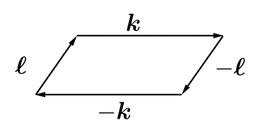
Given the form of the power spectrum (64) and the form of the trispectrum (69), we define the non-linear amplitude and the shape of the trispectrum . The most general shape is given by the parallelogram in the momentum space with two pairs of conjugate momenta, and an arbitrary angle between these pairs (see Fig. 1). We note that it corresponds to the parallelogram limit of the so-called “local" shape that was constrained by the Planck collaboration in Ref. [24]. For instance, in the limit (implying ), we obtain
| (70) |
which is nothing but , where
is the “local" shape given by Eq. (43) in Ref. [24]. Assuming the standard power spectrum then yields the universal shape function
| (71) |
depending essentially on the ratio between the lengths of the parallelogram’s sides in Fig. 1. The amplitude of the trispectrum does not depend on the angle between the sides but only on their relative lengths, and it scales with the overall size of the parallelogram as the power spectrum cubed.
The Planck collaboration did not find evidence for a non-zero primordial trispectrum and constrained the amplitude , which is therefore for the moment largely unconstrained. However, the minimal prediction we foresee in our context of quantizing the background as well as the perturbations is that of a non vanishing signal, with an amplitude to be determined in a model-dependent way, for the very specific shape (71).
Methods for analysing the shapes of non-Gaussianity with cosmic microwave background and large scale structure data are well-developed, in particular for the case of bispectrum (see, e.g. [25] for a review). The case of the CMB trispectrum has been investigated in [26, 27] (see also Ref. [28] for detection issues). On the other hand, obtaining the theoretical value of the amplitude requires choosing a specific model and calculating the value of via Eq. (54). We stress again that this calculation can be performed both for inflationary as well as alternative models, potentially leading to distinct predictions.
V.4 Heisenberg picture
Some calculations may be more easily performed in the Heisenberg picture. Making use of the definition , we obtain the Heisenberg form of , which we denote by , namely
| (72) |
Upon using the expansion discussed above, we get
| (73) |
where we omitted the projector , acting on . Switching to the position representation, we finally get
| (74) |
where is a Gaussian field evolving according to the BO dynamics. From Eq. (74), it is evident that the non-Gaussianity of is very non-local.
VI Discussion
In this work we have derived a perturbation theory of the multiverse dynamics of quantum cosmological systems, starting from the first principles. We showed that the multiverse states develop inevitably in the quantum models of primordial universe when the interaction between the background and the perturbation is carefully taken into account. The main result is the derivation of the general formulas (55) and (54), which give an analytical form of the multiverse correction to the initial Born-Oppenheimer state of the universe, that is, the tensor-product of a background state and an adiabatic vacuum for the perturbation.
It was then shown that these new cosmological states describe the primordial fluctuations with non-Gaussian features of a very specific form. Namely, we found that the connected correlation functions of even order do not vanish, and evaluated the the lowest-order contribution, i.e. the trispectrum. We found that the its amplitude depends on the scale-invariant function and on the power spectrum of the BO state. Assuming the latter to be approximately scale-invariant, a universal shape function of the trispectrum was derived. The numerical value of the expected amplitude of non-Gaussianity, not calculable in a general way, must be obtained by setting a specific model for the primordial universe. An earlier evaluation was provided in a simplified bouncing model [16] containing only two background states. Whether similar conclusion will hold in generic inflationary models still remains to be verified. Nevertheless, we expect that, had a quantum gravity phase preceded an inflationary phase, the non-Gaussianities produced by the quantum gravity phase should have survived the inflation and may not have been simply washed out.
The density fluctuations inside other branches of the primeval multiverse alter via gravitational interaction the geometry of our Universe, causing small but in principle measurable curvature imprints. When superimposed on the linear structure, these imprints produce a distinct pattern of non-Gaussianities, making the multiverse scenario a testable physical theory. It must be noted, however, that no signal of non-Gaussianities has been detected so far. The Planck collaboration has put constraints on some shapes of the bispectrum and the trispectrum [24]. However, these constraints do not concern the trispectrum obtained from the multiverse dynamics and a new analysis of the available data involving the obtained shape function is necessary. Various ongoing and planned CMB experiments will significantly improve polarization sensitivity and measurements down to smaller scales, further constraining non-Gaussianities [29, 30, 31].
Let us note that a potential detection of the non-Gaussianities of the predicted shape would strongly enforce the evidence for quantum gravity effects in the primordial universe despite the fact that the primordial gravity waves that are widely held as a clean quantum gravity signature, remain undetected.
The next step in the development of the multiverse formalism is to determine the explicit value of the function defined in Eq. (54). We emphasize that the developed perturbation theory does not assume any specific quantum cosmological model and hence, the formula (54) can be evaluated in various ways. In subsequent forthcoming work, we will apply our present formalism to a bouncing model based on analytically determined quantum background solutions [22] as well as to a simple inflationary model.
Let us finish this work by noting that the existence of multiverse states, though completely correct and even necessary from the point of view of quantum formalism, raise difficult interpretational issues. The existence of multiple branches in the primordial multiverse, and their imprints on the observed cosmological fluctuations in our branch, prompt questions such as: Did these other branch universes really exist? Do they still exist? Is the wave function a tangible, physical entity or, is it merely a mathematical construct that should not be confused with the physical reality? Presently, none of these questions can be really answered, however, it is plausible that our framework could to some extent be useful in addressing some of these and similar issues.
Acknowledgements.
P.M. acknowledges the support of the National Science Centre (NCN, Poland) under the Research Grant 2018/30/E/ST2/00370.References
- Hartle and Hawking [1983] J. B. Hartle and S. W. Hawking, Wave Function of the Universe, Phys. Rev. D 28, 2960 (1983).
- Vilenkin [1983] A. Vilenkin, The Birth of Inflationary Universes, Phys. Rev. D 27, 2848 (1983).
- Halliwell and Hawking [1985] J. J. Halliwell and S. W. Hawking, The Origin of Structure in the Universe, Phys. Rev. D 31, 1777 (1985).
- Pinho and Pinto-Neto [2007] E. J. C. Pinho and N. Pinto-Neto, Scalar and vector perturbations in quantum cosmological backgrounds, Phys. Rev. D 76, 023506 (2007), arXiv:hep-th/0610192 .
- Peter et al. [2006] P. Peter, E. J. C. Pinho, and N. Pinto-Neto, Gravitational wave background in perfect fluid quantum cosmologies, Phys. Rev. D 73, 10.1103/physrevd.73.104017 (2006).
- Peter and Pinto-Neto [2008] P. Peter and N. Pinto-Neto, Cosmology without inflation, Phys. Rev. D 78, 063506 (2008), arXiv:0809.2022 [gr-qc] .
- Lehners [2008] J.-L. Lehners, Ekpyrotic and Cyclic Cosmology, Phys. Rept. 465, 223 (2008), arXiv:0806.1245 [astro-ph] .
- Małkiewicz and Miroszewski [2021] P. Małkiewicz and A. Miroszewski, Dynamics of primordial fields in quantum cosmological spacetimes, Phys. Rev. D 103, 10.1103/physrevd.103.083529 (2021).
- Pinto-Neto and Fabris [2013] N. Pinto-Neto and J. C. Fabris, Quantum cosmology from the de Broglie-Bohm perspective, Class. Quant. Grav. 30, 143001 (2013), arXiv:1306.0820 [gr-qc] .
- Ashtekar et al. [2009] A. Ashtekar, W. Kaminski, and J. Lewandowski, Quantum field theory on a cosmological, quantum space-time, Phys. Rev. D 79, 064030 (2009).
- Gomar et al. [2014] L. C. Gomar, M. Fernández-Méndez, G. A. M. Marugán, and J. Olmedo, Cosmological perturbations in hybrid loop quantum cosmology: Mukhanov-sasaki variables, Phys. Rev. D 90, 10.1103/physrevd.90.064015 (2014).
- Kamenshchik et al. [2013] A. Y. Kamenshchik, A. Tronconi, and G. Venturi, Inflation and quantum gravity in a born-oppenheimer context, Phys. Lett. B 726, 518 (2013).
- Chataignier and Krämer [2021] L. Chataignier and M. Krämer, Unitarity of quantum-gravitational corrections to primordial fluctuations in the born-oppenheimer approach, Phys. Rev. D 103, 066005 (2021).
- Bini et al. [2013] D. Bini, G. Esposito, C. Kiefer, M. Krämer, and F. Pessina, On the modification of the cosmic microwave background anisotropy spectrum from canonical quantum gravity, Phys. Rev. D 87, 104008 (2013).
- Kiefer [2007] C. Kiefer, Quantum Gravity, 2nd ed. (Oxford University Press, New York, 2007).
- Bergeron et al. [2024a] H. Bergeron, P. Malkiewicz, and P. Peter, Quantum entanglement and non-Gaussianity in the primordial Universe, Phys. Rev. D 110, 043512 (2024a), arXiv:2405.09307 [gr-qc] .
- Ellis and Stoeger [1987] G. F. R. Ellis and W. Stoeger, The ’fitting problem’ in cosmology, Class. Quant. Grav. 4, 1697 (1987).
- Livio and Rees [2018] M. Livio and M. J. Rees, Fine-Tuning, Complexity, and Life in the Multiverse, (2018), arXiv:1801.06944 [physics.hist-ph] .
- Tegmark and Rees [1998] M. Tegmark and M. J. Rees, Why is the Cosmic Microwave Background fluctuation level 10**(-5)?, Astrophys. J. 499, 526 (1998), arXiv:astro-ph/9709058 .
- Linde [2017] A. Linde, A brief history of the multiverse, Rept. Prog. Phys. 80, 022001 (2017), arXiv:1512.01203 [hep-th] .
- Everett [1957] H. Everett, Relative state formulation of quantum mechanics, Rev. Mod. Phys. 29, 454 (1957).
- Bergeron et al. [2024b] H. Bergeron, J.-P. Gazeau, P. Małkiewicz, and P. Peter, New class of exact coherent states: Enhanced quantization of motion on the half line, Phys. Rev. D 109, 023516 (2024b), arXiv:2310.16868 [quant-ph] .
- Lewis [2011] A. Lewis, The real shape of non-Gaussianities, JCAP 10, 026, arXiv:1107.5431 [astro-ph.CO] .
- Akrami et al. [2020] Y. Akrami et al. (Planck), Planck 2018 results. IX. Constraints on primordial non-Gaussianity, Astron. Astrophys. 641, A9 (2020), arXiv:1905.05697 [astro-ph.CO] .
- Liguori et al. [2010] M. Liguori, E. Sefusatti, J. R. Fergusson, and E. P. S. Shellard, Primordial non-Gaussianity and Bispectrum Measurements in the Cosmic Microwave Background and Large-Scale Structure, Adv. Astron. 2010, 980523 (2010), arXiv:1001.4707 [astro-ph.CO] .
- Smith et al. [2015] K. M. Smith, L. Senatore, and M. Zaldarriaga, Optimal analysis of the CMB trispectrum, (2015), arXiv:1502.00635 [astro-ph.CO] .
- Hindmarsh et al. [2010] M. Hindmarsh, C. Ringeval, and T. Suyama, The CMB temperature trispectrum of cosmic strings, Phys. Rev. D 81, 063505 (2010), arXiv:0911.1241 [astro-ph.CO] .
- Anil Kumar et al. [2022] N. Anil Kumar, G. Sato-Polito, M. Kamionkowski, and S. C. Hotinli, Primordial trispectrum from kinetic Sunyaev-Zel’dovich tomography, Phys. Rev. D 106, 063533 (2022), arXiv:2205.03423 [astro-ph.CO] .
- Abazajian et al. [2016] K. N. Abazajian et al. (CMB-S4), CMB-S4 Science Book, First Edition, (2016), arXiv:1610.02743 [astro-ph.CO] .
- Ade et al. [2019] P. Ade et al. (Simons Observatory), The Simons Observatory: Science goals and forecasts, JCAP 02, 056, arXiv:1808.07445 [astro-ph.CO] .
- Alvarez et al. [2019] M. Alvarez et al., PICO: Probe of Inflation and Cosmic Origins, Bull. Am. Astron. Soc. 51, 194 (2019), arXiv:1908.07495 [astro-ph.IM] .