Potential Score Matching: Debiasing Molecular Structure Sampling with Potential Energy Guidance

Abstract

The ensemble average of physical properties of molecules is closely related to the distribution of molecular conformations, and sampling such distributions is a fundamental challenge in physics and chemistry. Traditional methods like molecular dynamics (MD) simulations and Markov chain Monte Carlo (MCMC) sampling are commonly used but can be time-consuming and costly. Recently, diffusion models have emerged as efficient alternatives by learning the distribution of training data. Obtaining an unbiased target distribution is still an expensive task, primarily because it requires satisfying ergodicity. To tackle these challenges, we propose Potential Score Matching (PSM), an approach that utilizes the potential energy gradient to guide generative models. PSM does not require exact energy functions and can debias sample distributions even when trained on limited and biased data. Our method outperforms existing state-of-the-art (SOTA) models on the Lennard-Jones (LJ) potential, a commonly used toy model. Furthermore, we extend the evaluation of PSM to high-dimensional problems using the MD17 and MD22 datasets. The results demonstrate that molecular distributions generated by PSM more closely approximate the Boltzmann distribution compared to traditional diffusion models.

1 Introduction

Physical quantities of interest, such as free energy, are often determined by ensemble averages and are intrinsically linked to the distribution of molecular conformations [2, 34]. Traditional techniques for quantifying these physical quantities, notably Markov Chain Monte Carlo (MCMC) sampling and Molecular Dynamics (MD), are well-established [15, 25, 29]. However, these methods are computationally intensive, particularly for systems with high-dimensional molecules.

Unlike the inherently sequential sampling of MD and MCMC, generative models, especially diffusion models, have emerged as efficient alternatives for generating independent and identically distributed (i.i.d.) samples [33, 16, 32, 30, 9, 38, 40, 17, 37]. One such approach is Denoising Score Matching (DSM) [33]. These models apply a score function to learn the data distribution, which is particularly useful in molecular systems where the equilibrium distribution adheres to the Boltzmann distribution. This distribution can be expressed as $p(\bm{x})\propto e^{-\mathcal{E}(\bm{x})/(k_{B}T)}$, with $k_{B}$ denoting the Boltzmann constant, $T$ the temperature, and $\mathcal{E}(\bm{x})$ the energy function of the system. Constructing a dataset that follows the Boltzmann distribution remains a challenging task, and failure to provide unbiased training data can result in DSM overfitting to a biased distribution, leading to inaccurate observables.

Recent advances in generative modeling have sought to incorporate the principles of the Boltzmann distribution for improved molecular sampling [39, 37, 4, 6, 8]. Techniques such as the Denoising Diffusion Sampler (DDS) and the Path Integral Sampler (PIS) [42, 35] have been developed to amortize the computational expense of traditional MCMC and MD methods, facilitating learning processes that do not necessitate equilibrium data. These methods typically rely on integration paths derived from ordinary differential equations (ODEs) and stochastic differential equations (SDEs), which, despite being innovative, still involve substantial computational time. The Iterated Denoising Energy Matching (iDEM) framework [1] represents another stride forward, employing energy functions for data generation and introducing energy-guided sampling independent of the initial distribution. The complexity of its iterative loops and the absence of predefined initial data increase the computational overhead in high dimensional space, and at larger time scales, iDEM’s sampling efficiency diminishes, demanding a greater number of samples to obtain precise outcomes. A more recent approach, Target Score Matching (TSM) [4], integrates energy information with DSM to enable sampling from designated energy functions under the assumption of data unbiasedness.

Table 1: Comparison of molecular sampling methods and their properties.

	Inference i.i.d. Samples	Doesn’t Require Exact Boltzmann Data for Training	Efficiency in High Dim.	Doesn’t Require Energy Function (Only Energy Labels)
MD/MCMC	$\times$	✓	$\times$	$\times$
DSM	✓	$\times$	✓	✓
DDS/PIS	✓	$\times$	$\times$	$\times$
iDEM	✓	✓	$\times$	$\times$
TSM	✓	$\times$	✓	✓
PSM (ours)	✓	✓	✓	✓

In this work, we introduce the Potential Score Matching (PSM) method, which incorporates potential energy derivatives into generative models to more closely align the sample distribution with the Boltzmann distribution. Furthermore, PSM requires only force labels for the reference structures and obviates the need for an explicit energy function. PSM leverages the characteristics of DSM to facilitate the generation of i.i.d. samples, offering a computationally efficient alternative to MD simulations. We provide a comparative analysis of PSM with related methodologies in Table 1. We also present a series of theoretical proofs demonstrating that PSM provides a more accurate estimation of the score function in the vicinity of $t=0$ when training data is biased and results in reduced variance near $t=0$. The performance of PSM is validated on both simple toy models, such as Lennard-Jones (LJ) potentials, and more complex, high-dimensional physical datasets, including MD17 and MD22. Our experimental results consistently indicate that PSM outperforms baseline models.

2 Preliminaries

2.1 Score-Based Generative Modeling

Diffusion models operate through a two-step process [16, 32]: (1) a forward diffusion process that incrementally adds noise to the data $\bm{x}_{0}$ until it converges to a Gaussian distribution at time $T$, and (2) a reverse denoising process that reconstructs samples using a learned score function. The forward process is defined by $\bm{x}_{t}=\alpha_{t}\bm{x}_{0}+\sigma_{t}\bm{\epsilon}$, where $\alpha_{t}$ and $\sigma_{t}$ are noise schedule coefficients, and $\bm{\epsilon}$ represents standard Gaussian noise. Two widely used frameworks are the variance-preserving (VP-SDE) and variance-exploding (VE-SDE) diffusion processes [33]. In VE-SDE, $\alpha_{t}=1$ and $\sigma_{t}=\sigma_{\text{min}}(\sigma_{\text{max}}/\sigma_{\text{min}})^{t}$, while in VP-SDE, $\alpha_{t}=e^{-\frac{1}{2}\int_{0}^{t}\beta_{s}ds}$ and $\sigma_{t}=\sqrt{1-e^{-\int_{0}^{t}\beta_{s}ds}}$. Both VP and VE can be abstracted as $\mathrm{d}\boldsymbol{x}_{t}=f(\boldsymbol{x}_{t},t)\mathrm{~d}t+g(t)\mathrm{~d}W_{t}$. Following this, the reverse process, solves the reverse SDE from $T$ back to 0 is

$$\mathrm{d}\boldsymbol{x}_{t}=\left(f(\boldsymbol{x}_{t},t)-g^{2}(t)\nabla_{\boldsymbol{x}_{t}}\log q_{t}\left(\boldsymbol{x}_{t}\right)\right)\mathrm{~d}t+g(t)\mathrm{~d}W_{t}\,.$$ (1)

The term $\nabla_{\boldsymbol{x}_{t}}\log q_{t}(\cdot)$, known as the “score" function at time $t$, remains unknown and is estimated through training a neural network $\boldsymbol{s}_{\theta}$, parameterized by $\theta$, or leveraging the relationship $s_{\theta}=-\frac{\boldsymbol{\epsilon}_{\theta}}{\sigma_{t}}$ and training $\boldsymbol{\epsilon}_{\theta}\left(\boldsymbol{x}_{t},t\right)$. The training objective is formulated as:

$$\min_{\theta}\mathbb{E}_{t,\boldsymbol{x}_{t},\bm{\epsilon}}\left[\lambda(t)\left\|\boldsymbol{\epsilon}_{\theta}\left(\boldsymbol{x}_{t},t\right)+\sigma_{t}\nabla_{\boldsymbol{x}_{t}}\log q_{t}\left(\boldsymbol{x}_{t}\right)\right\|_{2}^{2}\right]\Leftrightarrow\min_{\theta}\mathbb{E}_{t,\boldsymbol{x}_{t},\boldsymbol{\epsilon}}\left[\lambda(t)\left\|\boldsymbol{\epsilon}_{\theta}\left(\boldsymbol{x}_{t},t\right)-\boldsymbol{\epsilon}\right\|_{2}^{2}\right],$$ (2)

where the expectation $\mathbb{E}$ is taken over time $t$, sampled from a uniform distribution $\mathcal{U}([0,1])$, the noised data points $\boldsymbol{x}_{t}$, sampled from the distribution $q(\boldsymbol{x}_{t}|\boldsymbol{x}_{0})$, and the noise $\boldsymbol{\epsilon}$, sampled from a standard Gaussian distribution. The function $\lambda(t)$ represents a weighting function that adjusts the importance of different time steps during the optimization process. In molecular systems, $\bm{x}_{t}$ often denotes atomic positions or, in some contexts, discrete atomic types. Diffusion models have become increasingly prevalent in the generation of molecular structures and the prediction of their properties [9].

2.2 Boltzmann Distribution

Molecular systems at equilibrium are typically characterized by the Boltzmann distribution, with the target distribution given by $p(\bm{x}_{0})\propto e^{-\mathcal{E}(\bm{x}_{0})/(k_{B}T)}$. A profound connection exists between the score function utilized in diffusion models and the system’s potential energy, as $\nabla\log p(\bm{x}_{0})\propto-\nabla\mathcal{E}(\bm{x}_{0})/(k_{B}T)$. Nevertheless, harnessing the Boltzmann distribution for generative modeling poses several challenges. For molecular systems with analytically specified energy functions, the exact distribution is the normalized form of the Boltzmann factor. The normalization constant, typically expressed as an integral over all possible configurations, is often intractable and eludes a closed-form expression. Recent research has integrated energy considerations into score-based model variants to improve molecular predictions. Innovations include the introduction of an equivariant energy-guided SDE [3] and novel score functions [18, 11, 30, 36, 1]. Additionally, attaining equilibrium presupposes ergodicity in the system, which is ensured by simulating molecular trajectories over extended periods. This requirement poses computational and temporal demands. In our approach, we address these issues by harnessing the derivatives of energy to facilitate this process.

3 Potential Score Matching in Molecular Systems

In this section, we introduce our Potential Score Matching (PSM) method, which leverages the derivatives of potential energy to efficiently approximate the Boltzmann distribution. Consider a training sample $\bm{x}_{0}$ drawn from the dataset, subjected to a noise injection process defined as $\bm{x}_{t}=\alpha_{t}\bm{x}_{0}+\sigma_{t}\bm{\epsilon}$, where $\sigma_{t}$ is a time-dependent noise schedule. We formalize the representation of the score function for molecules that adhere to the Boltzmann distribution as follows:

Theorem 1.

In a molecular system where molecules follow the distribution $p(\bm{x}_{0})\propto e^{-\mathcal{E}/(k_{B}T)}$, given $\bm{x}_{t}=\alpha_{t}\bm{x}_{0}+\sigma_{t}\epsilon$, the score function at time $t$ is an expectation of the force,

$$\nabla_{\bm{x}_{t}}\log p(\bm{x}_{t})=\frac{1}{\alpha_{t}}\mathbb{E}_{\bm{x}_{0}|\bm{x}_{t}}\left[\frac{-\nabla_{\bm{x}_{0}}\mathcal{E}}{k_{B}T}\right]=\frac{1}{\alpha_{t}}\mathbb{E}_{\bm{x}_{0}|\bm{x}_{t}}\left[\frac{\bm{F}}{k_{B}T}\right]\,,$$ (3)

where $\mathcal{E}$ and $\bm{F}$ represent the potential energy and force of $\bm{x}_{0}$, respectively. Thus, the PSM loss is defined as

$$\mathcal{L}_{s\text{-model}} =\mathbb{E}_{t\sim\mathcal{U}(0,1)}\mathbb{E}_{\bm{x}_{t}\sim p(\bm{x}_{t}|\bm{x}_{0})}\mathbb{E}_{\bm{x}_{0}}\left[\lambda(t)\left\|\bm{s}_{\theta}(\bm{x}_{t},t)-\frac{1}{\alpha_{t}}(-\frac{\nabla_{\bm{x}_{0}}\mathcal{E}}{k_{B}T})\right\|^{2}\right]$$ (4)

$$=\mathbb{E}_{t\sim\mathcal{U}(0,1)}\mathbb{E}_{\bm{x}_{t}\sim p(\bm{x}_{t}|\bm{x}_{0})}\mathbb{E}_{\bm{x}_{0}}\left[\lambda(t)\left\|\bm{s}_{\theta}(\bm{x}_{t},t)-\frac{1}{\alpha_{t}}\frac{\bm{F}}{k_{B}T}\right\|^{2}\right],$$

where $\mathcal{U}(0,1)$ denotes a uniform distribution, and $p(\bm{x}_{t}|\bm{x}_{0})$ is the conditional probability distribution of the noise-injected sample given the $\bm{x}_{0}$.

The proof of Theorem 1 is provided in Appendix B.1. The loss function (4), also known as the $``$score loss$"$, can be further expressed in terms of the $``\bm{x}_{0}$ loss$"$ and $``\epsilon$ loss$"$, as detailed in [24]:

$$\mathcal{L}_{\bm{x}_{0}\text{-model}}=\mathbb{E}_{t\sim\mathcal{U}(0,1)}\mathbb{E}_{\bm{x}_{t}\sim q(\bm{x}_{t}|\bm{x}_{0})}\mathbb{E}_{\bm{x}_{0}}\left[\lambda(t)\left\|\mathcal{D}_{\theta}-\bm{x}_{t}-\frac{\sigma_{t}^{2}}{\alpha_{t}}\frac{\nabla_{\bm{x}_{0}}\mathcal{E}(\bm{x}_{0})}{k_{B}T}\right\|_{2}^{2}\right]\,,$$ (5)

$$\mathcal{L}_{\bm{\epsilon}\text{-model}}=\mathbb{E}_{t\sim\mathcal{U}(0,1)}\mathbb{E}_{\bm{x}_{t}\sim q(\bm{x}_{t}|\bm{x}_{0})}\mathbb{E}_{\bm{x}_{0}}\left[\lambda(t)\left\|\bm{\epsilon}_{\theta}(\bm{x}_{t},t)+\frac{\sigma_{t}}{\alpha_{t}}\frac{\bm{F}}{k_{B}T}\right\|_{2}^{2}\right]\,,$$ (6)

where $\mathcal{D}_{\theta}$ and $\bm{\epsilon}_{\theta}$ are neural networks designed to approximate the original data point $\bm{x}_{0}$ and the noise term $\bm{\epsilon}$, respectively. Recall that the formulas for the VESDE forward process that $\alpha_{t}=1$, the loss can be written as $\mathcal{L}=\mathbb{E}_{t\sim U(0,1)}\mathbb{E}_{\bm{x}_{t}\sim p(\bm{x}_{t}|\bm{x}_{0})}\mathbb{E}_{\bm{x}_{0}}\left[\lambda(t)\|\bm{s}_{\theta}(\bm{x}_{t},t)-\frac{\bm{F}}{k_{B}T}\|^{2}\right]$. For simplicity, we denote $k_{B}T=1$ in this section.

Related ideas are explored in Target Score Matching (TSM) [4], which utilizes an explicit energy function to model the score. Building on this concept, we link energy derivatives to the score function and present Potential Score Matching (PSM), which embodies the aforementioned score representation. By utilizing force labels as a proxy to the Boltzmann distribution, our approach reduces computational costs. Our work expands upon TSM, moving from toy models with explicit energy functions to real molecular systems, by leveraging force labels instead of complete energy expressions. Moreover, our theoretical findings assert that PSM remains robust even when trained on data that does not adhere to the Boltzmann distribution, thereby correcting biases in the training dataset and yielding samples that more closely resemble the true distribution.

Now we denote that $p(\bm{x}_{0})$ is the Boltzmann distribution and $q(\bm{x}_{0})$ is the data distribution. Ideally, $p(\bm{x}_{0})$ should coincide with $q(\bm{x}_{0})$; however, when starting with a biased distribution, these two may not be equal. We demonstrate that PSM can provide a superior training process in terms of data fidelity, regardless of whether the training data is biased or unbiased. Since $\nabla_{\bm{x}_{t}}\log p(\bm{x}_{t})=\int p(\bm{x}_{0}|\bm{x}_{t})\nabla_{\bm{x}_{0}}\log p(\bm{x}_{0})d\bm{x}_{0}$, the optimal solution satisfies:

$$\mathrm{argmin}_{\bm{s}(\cdot,\cdot)}\mathbb{E}_{p(\bm{x}_{0})}\mathbb{E}_{p(\bm{x}_{t}|\bm{x}_{0})}\|\bm{s}(\bm{x}_{t},t)-\nabla_{\bm{x}_{t}}\log p(\bm{x}_{t})\|=\mathbb{E}_{p(\bm{x}_{0}|\bm{x}_{t})}\left[\nabla_{\bm{x}_{0}}\log p(\bm{x}_{0})\right].$$ (7)

Thus, the ground truth is given by $\mathbb{E}_{p\left(\bm{x}_{0}\mid\bm{x}_{t}\right)}\left[\nabla\log p\left(\bm{x}_{0}\right)\right],$ and the Denoising Score Matching (DSM) method learns this same expectation. The following theorem establishes that at small time steps, PSM more closely approximates the Boltzmann distribution than DSM. A detailed explanation is provided in Appendix B.2.

Theorem 2.

For the Boltzmann distribution $p(\bm{x}_{0})$, the data distribution $q(\bm{x}_{0})$, and small $t$, PSM learns a more accurate score function than DSM,

$$\left\|\underbrace{\mathbb{E}_{q\left(\bm{x}_{0}\mid\bm{x}_{t}\right)}\left[\nabla\log p\left(\bm{x}_{0}\right)\right]}_{\textnormal{PSM}}-\underbrace{\mathbb{E}_{p\left(\bm{x}_{0}\mid\bm{x}_{t}\right)}\left[\nabla\log p\left(\bm{x}_{0}\right)\right]}_{\textnormal{Ground Truth}}\right\|_{2}^{2}\leqslant\left\|\underbrace{\mathbb{E}_{q\left(\bm{x}_{0}\mid\bm{x}_{t}\right)}\left[\nabla\log q\left(\bm{x}_{0}\right)\right]}_{\textnormal{DSM}}-\underbrace{\mathbb{E}_{p\left(\bm{x}_{0}\mid\bm{x}_{t}\right)}\left[\nabla\log p\left(\bm{x}_{0}\right)\right]}_{\textnormal{Ground Truth}}\right\|_{2}^{2}.$$ (8)

Furthermore, denoting the right-hand side as $\|I_{1}\|_{2}^{2}$ and the left-hand side as $\|I_{2}\|_{2}^{2}$, the difference between these two terms satisfies $\|I_{2}\|_{2}^{2}-\|I_{1}\|_{2}^{2}\geq\|I_{3}\|_{2}^{2}+O(t^{3})$, where $I_{3}=I_{3}(\bm{x}_{0},\bm{x}_{t})>0$ in a neighborhood of $t=0$.

Recent works [41, 30] have indicated that during the training of traditional diffusion models, there is a tendency to encounter excessively large Lipschitz constants and significant variance in relation to the time variable near $t=0$. This behavior has the potential to destabilize the training process. We demonstrate that PSM effectively mitigates these issues at $t=0$ and provide theoretical support from the perspectives of variance and Lipschitz problems in Appendix B.3. Considering the instability of DSM near $t=0$, we propose a weighted combination of both losses, referred to as $``$Piecewise Loss$"$ and $``$Piecewise-Weighted Loss$"$. These methods prioritize PSM for small $t$ while favoring DSM at larger time values.

Piecewise loss.

Assuming $k_{B}T=1$, we use the force loss ((6)) exclusively for $t\in[0,t_{p}]$, while employing DSM for $t>t_{p}$ as follows:

$$\bm{s}\left(\bm{x}_{t},t\right)=\begin{cases}\frac{1}{\alpha_{t}}\mathbb{E}_{\bm{x}_{0}\mid\bm{x}_{t}}\left[\nabla_{\bm{x}_{0}}\log p\left(\bm{x}_{0}\right)\right],&\text{if }t<t_{p},\\ \mathbb{E}_{\bm{x}_{0}\mid\bm{x}_{t}}\left[\nabla_{\bm{x}_{t}}\log p\left(\bm{x}_{t}\mid\bm{x}_{0}\right)\right],&\text{if }t\in[t_{p},1].\end{cases}$$ (9)

Piecewise Weighted loss.

Since $\bm{s}\left(\bm{x}_{t},t\right)=\mathbb{E}_{\bm{x}_{0}\mid\bm{x}_{t}}\left[\frac{1}{\alpha_{t}}\nabla_{\bm{x}_{0}}\log p\left(\bm{x}_{0}\right)\right]=\mathbb{E}_{\bm{x}_{0}\mid\bm{x}_{t}}\left[\nabla_{\bm{x}_{t}}\log p\left(\bm{x}_{t}\mid\bm{x}_{0}\right)\right]=\mathbb{E}_{\bm{x}_{0}\mid\bm{x}_{t}}\left[\frac{\bm{x}_{0}-\bm{x}_{t}}{\sigma_{t}^{2}}\right]\,,$ we consider another form of the score

$$s\left(\bm{x}_{t},t\right)=E_{\bm{x}_{0}\mid\bm{x}_{t}}\left[\omega_{t}\frac{1}{\alpha_{t}}\nabla_{\bm{x}_{0}}\log p\left(\bm{x}_{0}\right)+\left(1-\omega_{t}\right)\frac{\bm{x}_{0}-\bm{x}_{t}}{\sigma_{t}^{2}}\right]\,,$$ (10)

and the the loss is $\mathcal{L}=\mathbb{E}_{t,\bm{x}_{t},\bm{x}_{0}}\left[\lambda(t)\left\|-\frac{\bm{\epsilon}_{\theta}\left(\bm{x}_{t},t\right)}{\sigma_{t}}+\frac{\omega_{t}}{\alpha_{t}}\bm{F}-(1-\omega_{t})\frac{\bm{x}_{0}-\bm{x}_{t}}{\sigma_{t}^{2}}\right\|_{2}^{2}\right]\,.$ We choose $\omega_{t}$ as a time-varying function which satisfies that $\omega_{0}=1$ and $\omega_{1}=0$. For example, $\omega_{t}=\text{sigmoid}(50(t-0.05)),\,t\in[0,0.1]$ and $\omega_{t}=0$ when $t\in[0.1,1]$. We can see that this loss is a generalization of $``$Piecewise loss$"$. With a random noise $\bm{\epsilon}$, the $``$Piecewise loss$"$ and the $``$Piecewise Weighted loss$"$ can be unified as

$$\mathcal{L}_{\text{PSM}}=\mathbb{E}_{t,\bm{x}_{t},\bm{x}_{0}}\left[\|\bm{\epsilon}_{\theta}(\bm{x}_{t},t)-((1-\omega_{t})\bm{\epsilon}_{1}+\omega_{t}\bm{\epsilon}_{2})\|_{2}^{2}\right]\,,\,\text{where}\,\bm{\epsilon}_{1}=\bm{\epsilon}[t_{\text{dsm}}],\,\bm{\epsilon}_{2}=-\bm{F}[t_{\text{psm}}]\cdot\sigma_{t}\,,t_{\text{dsm}}\in[0,1]\setminus\{t_{\text{psm}}\}\,,$$ (11)

where $\bm{\epsilon}$ is a random noise, $t_{\text{psm}}$ refers to the noise adding time range using $\bm{F}$ as label, and $t_{\text{dsm}}$ is the element in its complement. The training process is shown in Algorithm 1.

Algorithm 1 Potential Score Matching

Network $\bm{\epsilon}_{\theta}$, total iteration $N$, data $\bm{x}_{0}$, forces $\bm{F}$, weight function $\omega_{t}$, noise schedule $\sigma_{t}$, and $\alpha_{t}$;

Select random noise $\bm{\epsilon}$;

Determine the time when the labels $\bm{F}$ and random noise $\bm{\epsilon}$ act, $t_{\text{psm}}$ and $t_{\text{dsm}}$.

while $n\leq N$ do

  $t\sim\mathcal{U}(0,1)$, $\bm{x}_{t}\sim\mathcal{N}(\alpha_{t}\bm{x}_{0},\sigma_{t}^{2})$, $\bm{\epsilon}_{1}=\bm{\epsilon}[t_{\text{dsm}}]$, $\bm{\epsilon}_{2}=-\frac{\bm{F}[t_{\text{psm}}]}{\alpha_{t}}\sigma_{t}$;

  $\mathcal{L}_{\text{PSM}}=\|\bm{\epsilon}_{\theta}(\bm{x}_{t},t)-((1-\omega_{t})\bm{\epsilon}_{1}+\omega_{t}\bm{\epsilon}_{2})\|_{2}^{2}$;

  $\theta\leftarrow\text{Update}(\theta,\nabla_{\theta}\mathcal{L}_{\text{PSM}})$;

end while

Our approach to incorporating force information is designed to be sample-efficient and does not impose constraints on the sampling methodology. It is compatible with common techniques employed in diffusion models, including the Euler method, Prediction-Correction (PC) method, and EDM [33, 19].

4 Experiments

Datasets.

We assess the performance of our proposed Potential Score Matching loss across various settings, including toy models like the Lennard-Jones (LJ) potential [20], and more intricate molecular systems such as MD17 and MD22. The LJ configurations, LJ-13 and LJ-55, consist of $13$ and $55$ atoms, respectively, arranged in a three-dimensional space. Historically, energy-based molecular sampling has largely concentrated on toy models [26, 1, 37, 4], but our approach extends this to higher-dimensional, real-world datasets, such as MD17 and MD22. MD17 contains molecular trajectories for different molecules, with $9$ to $21$ atoms, sampled at $500$ K, where the thermal energy $k_{B}T$ in the Boltzmann distribution equals $1$ kcal/mol. In contrast, MD22 poses a more demanding challenge due to its greater complexity, featuring molecular dynamics (MD) trajectories from a small peptide with $42$ atoms to a double-walled nanotube with $370$ atoms [7], sampled at $400$ to $500$ K with a time resolution of $1$ fs.

To demonstrate our method’s capability to correct biased training distributions and ensembles, we use Denoising Score Matching (DSM) [33] as a baseline and compare our results with those from iDEM and Flow AIS bootstrap (FAB) in toy model contexts [1, 26]. Our experiments primarily utilize biased training sets, employing the first $1,000$ frames for LJ data and the first $5,000$ frames for MD reference trajectories. Further investigation into the impact of dataset bias is conducted in the ablation study (Section 4.2).

Diffusion settings and network.

We evaluate our method using DSM, Piecewise, and Piecewise Weighted approaches, employing VESDE for denoising with equal time weight functions, $\lambda(t)=1$. In the Piecewise approach, PSM is applied for $t\leq 0.05$, while DSM is used for $t\in[0.05,1]$. In the Piecewise Weighted setting, the label is combined as $\omega_{t}\times\text{psm target}+(1-\omega_{t})\times\text{dsm target}$, where $\omega_{t}=\frac{1}{1+\exp(50(t-0.05))}.$ During training, we employ the $``\epsilon$-model$"$ loss function to learn the noise $\epsilon$.

Molecular systems often represent molecular structures as graphs, with atomic coordinates, numbers, and bonds defining a molecular graph. Symmetry and equivariance in these graph representations are crucial for accurate molecular interactions. We modify the Equiformer-v2 network based on [22] by incorporating the time variable as an additional input for training.

For sampling process, we use the Prediction-Correction (PC) sampler [33], where each prediction step are followed by one correction step. Additional experimental details, including hyperparameter settings, are available in Appendix C.

Evaluation metrics.

To evaluate the physical plausibility of the generated molecular conformations, we assess the stability of molecules in the MD17 dataset, following the method in [14]. A molecule is deemed unstable at time $T$ if:

$$\max_{(i,j)}\big{|}\|\bm{x}_{i}(T)-\bm{x}_{j}(T)\|-b_{ij}\big{|}>0.5,$$ (12)

where $b_{ij}$ is the equilibrium bond length between atoms $i$ and $j$. If no unstable molecules are detected, the dataset is considered stable. Moreover, we evaluate whether generated samples show an unbiased distribution by analyzing the statistical distribution of interatomic distances ($h(r)$), defined as:

$$h(r)=\frac{1}{N(N-1)}\sum_{i=1}^{N}\sum_{j\neq i}^{N}\delta(r-\|\bm{x}_{i}-\bm{x}_{j}\|),$$ (13)

where $r$ is the interatomic distance and $\delta$ is the Dirac delta function. This metric indicates whether the generated samples follow an unbiased molecular distribution. The mean absolute error (MAE) between the sampled $h(r)$ and reference data $h(r)$ also serves as a numerical comparison, providing more intuitive results.

For further numerical insights, we provide the Total Variation Distance (TVD) to measure the maximum distribution distance between sampled and reference data. For probability distributions $P$ and $Q$, TVD is defined as:

$$\text{TVD}(P,Q)=\frac{1}{2}\int_{\mathbb{R}^{d}}|P(\bm{x})-Q(\bm{x})|\,d\bm{x},$$

or equivalently for discrete distributions: $\text{TVD}(P,Q)=\frac{1}{2}\sum_{\bm{x}\in\mathcal{X}}|P(\bm{x})-Q(\bm{x})|.$ For datasets with available analytical energy expressions, we additionally provide energy distribution visualizations.

4.1 Main Results

4.1.1 Lennard-Jones Potential

The Lennard-Jones (LJ) potential encapsulates the fundamental principles of interatomic interactions: repulsive forces dominate at short distances, while attractive forces prevail at longer ranges. It is mathematically expressed as:

$$\mathcal{E}^{\mathrm{LJ}}(\bm{x})=\frac{1}{2\tau}\sum_{ij}\left(\left(\frac{r_{m}}{d_{ij}}\right)^{12}-2\left(\frac{r_{m}}{d_{ij}}\right)^{6}\right)\,.$$ (14)

$$\mathcal{E}^{\mathrm{osc}}(\bm{x})=\frac{1}{2}\sum_{i}\left\|\bm{x}_{i}-\bm{x}_{\mathrm{mean}}\right\|^{2}\,\quad\mathcal{E}^{\mathrm{tot}}=\mathcal{E}^{\mathrm{LJ}}(\bm{x})+\mathcal{E}^{\mathrm{osc}}(\bm{x})\,.$$ (15)

Here, $r_{m}$ and $\tau$ are constants that characterize the potential. In our experiments, we use the standard values $r_{m}=1$ and $\tau=1$, in line with previous studies [20, 1]. The term $\mathcal{E}^{\mathrm{osc}}$ represents the harmonic potential energy associated with particle displacements relative to the system’s center of mass, $\bm{x}_{\mathrm{mean}}$.

As indicated by (14), the function magnitude significantly increases when any interatomic distance $d_{ij}$ approaches zero, presenting substantial challenges, particularly in high-dimensional systems. To examine the effect of biased training data, we plot the histograms of interatomic distance distributions, $r=d_{ij}$, for LJ-13 and LJ-55, denoted as $h(r)$, in Figure 1. The results demonstrate that PSM effectively debiases samples when trained on biased distributions.

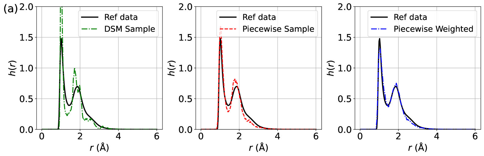
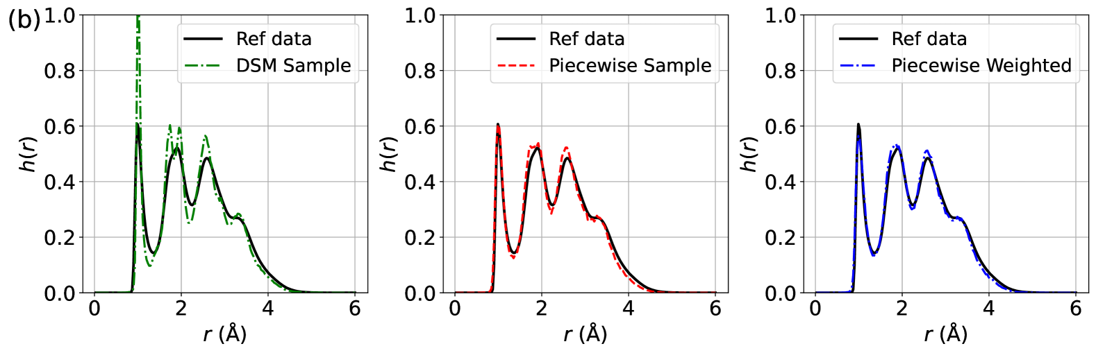
Figure 1: The distribution of interatomic distances $h(r)$ for LJ potential using biased training data with a sample size of $500$. (a) Comparison of $h(r)$ for DSM, Piecewise, and Piecewise Weighted losses (from left to right) against reference data for LJ-13; (b) Comparison of $h(r)$ for DSM, Piecewise, and Piecewise Weighted losses for LJ-55.

Compared to [1, 26], we also report the corresponding Wasserstein-2 ($\mathcal{W}$-2) distance and total variation distance (TVD) based on three sets of samples obtained by sampling with different random seeds. Table 2 presents these metric comparisons, where we test the LJ potential using a random $10\%$ subset of the reference data as the training set. Our experimental results show that it is applicable to the toy model and has advantages in high-dimensional situations. From another aspect, PSM also significantly reduces sampling time.

Table 2: Comparisons of PSM with FAB [26] and iDEM [1] on LJ-13 and LJ-55 results. Metrics include 2-Wasserstein distance and atomic distance TVD, evaluated on three different seeds.

	LJ-13 (39D)		LJ-55 (165D)
	Sample $\mathcal{W}$-2	Distance TVD	Sample $\mathcal{W}$-2	Distance TVD
FAB	$4.35\pm 0.001$	$0.252\pm 0.002$	$18.03\pm 1.21$	$0.24\pm 0.09$
iDEM	$\textbf{4.26}\pm 0.03$	$\textbf{0.044}\pm 0.001$	$16.128\pm 0.071$	$0.09\pm 0.01$
Piecewise	$4.287\pm 0.003$	$\underline{0.0582\pm 0.001}$	$\textbf{15.894}\pm\textbf{0.003}$	$\underline{0.047\pm 0.000}$
Piecewise-Weighted	$\underline{4.278\pm 0.001}$	$0.0585\pm 0.001$	$\underline{16.054\pm 0.008}$	$\textbf{0.023}\pm\textbf{0.002}$

4.1.2 Molecular Dynamical Data

Unlike other studies, our model proves effective on higher-dimensional datasets, specifically testing on MD17 and MD22 datasets. In MD17, we consider molecules such as Uracil (12 atoms), Naphthalene (10 atoms), Aspirin (21 atoms), Salicylic Acid (16 atoms), Malonaldehyde (9 atoms), Ethanol (9 atoms), and Toluene (15 atoms). This dataset provides molecules with properties like Cartesian coordinates (in Å), atomic numbers, total energies (in kcal/mol), and atomic forces (in kcal/mol/Å) at $500$ K, where the thermal energy $k_{B}T$ in the Boltzmann distribution corresponds to $1\,\text{kcal/mol}$. Additionally, we test the MD22 benchmark dataset, which includes Ac-Ala3-NHMe ($42$ atoms), Docosahexaenoic Acid (DHA) ($56$ atoms), Stachyose ($87$ atoms), DNA base pair (AT-AT) ($60$ atoms), DNA base pair (AT-AT-CG-CG) ($118$ atoms), Buckyball catcher ($148$ atoms), and Double-walled nanotube ($370$ atoms).

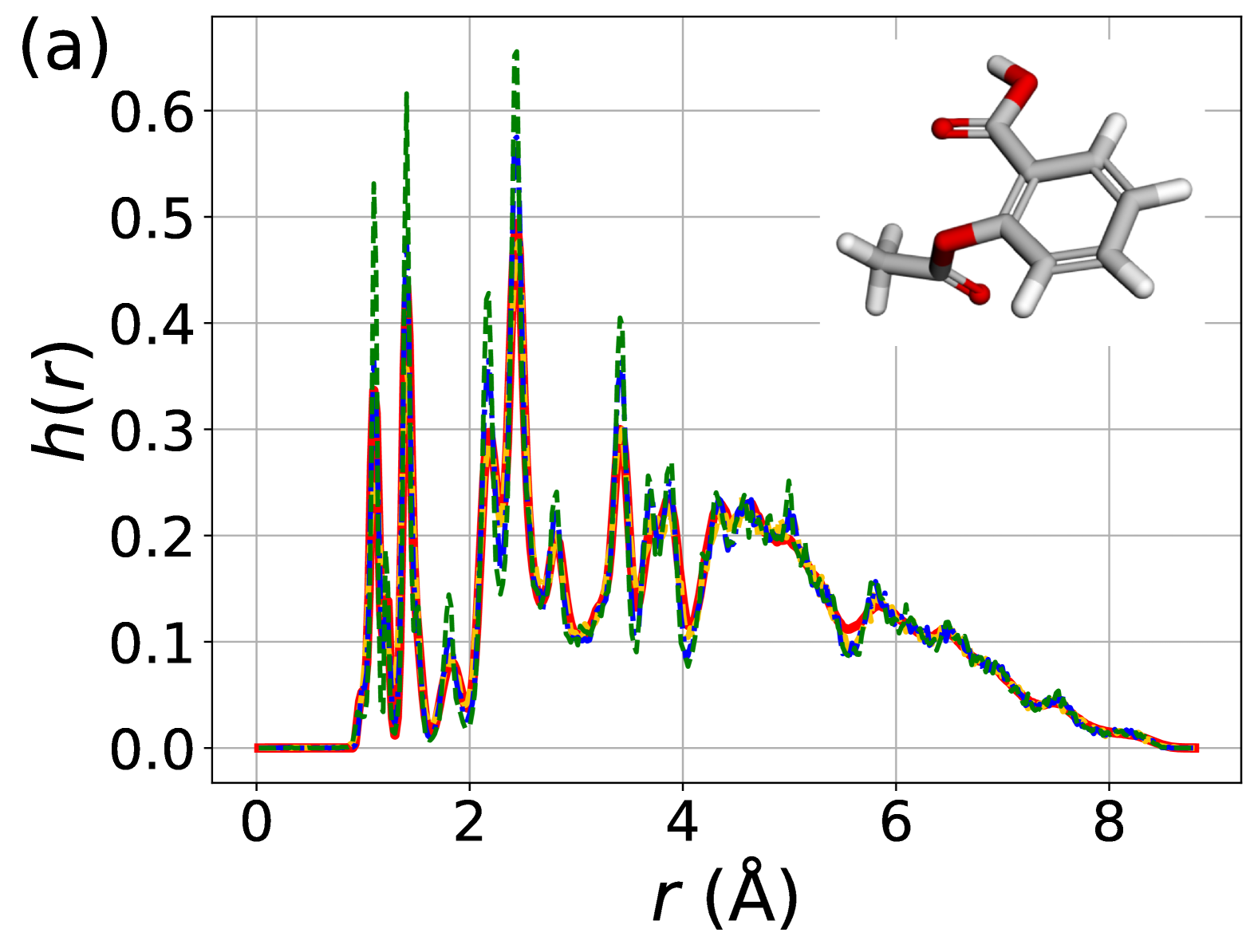
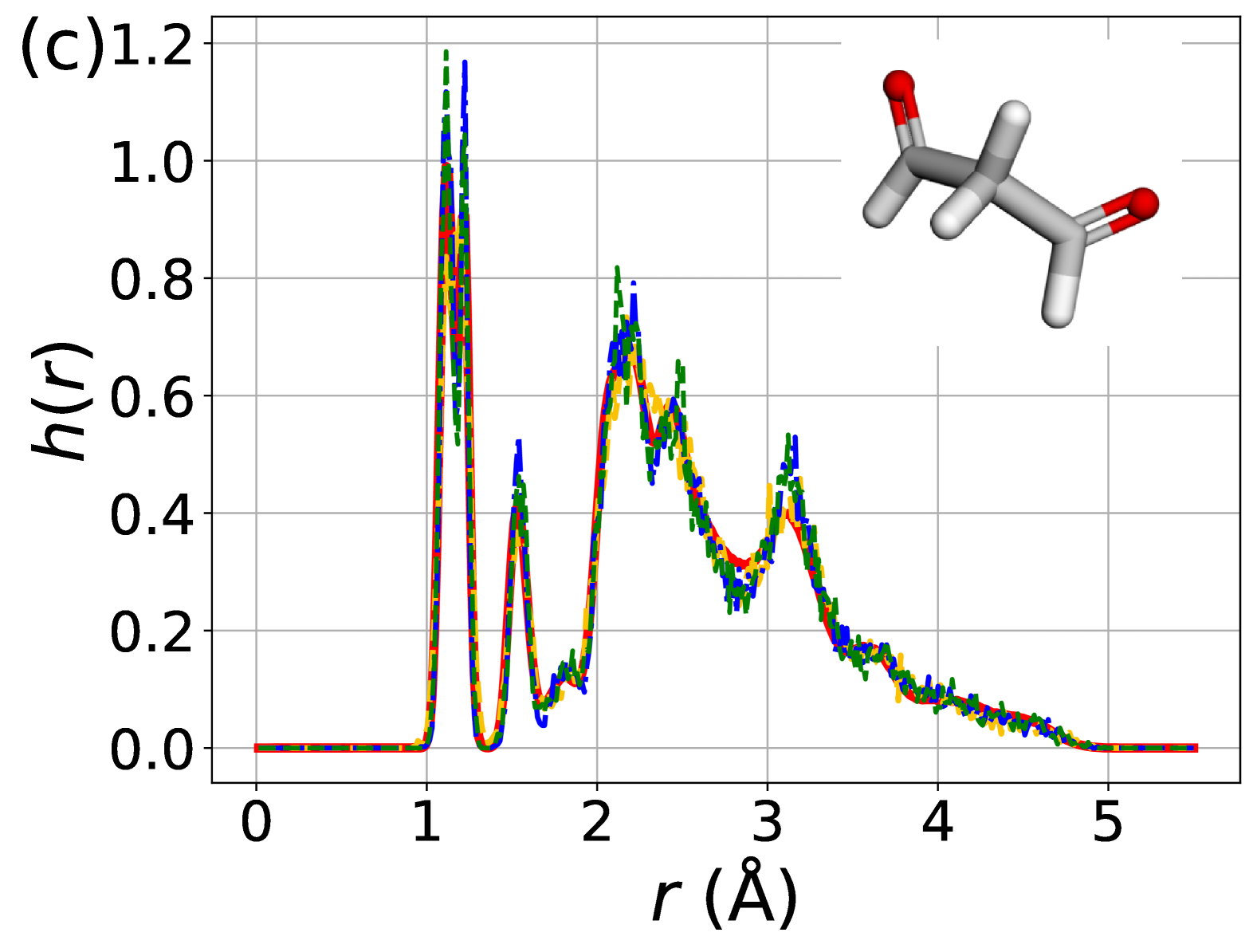
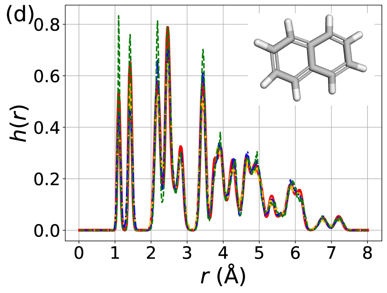
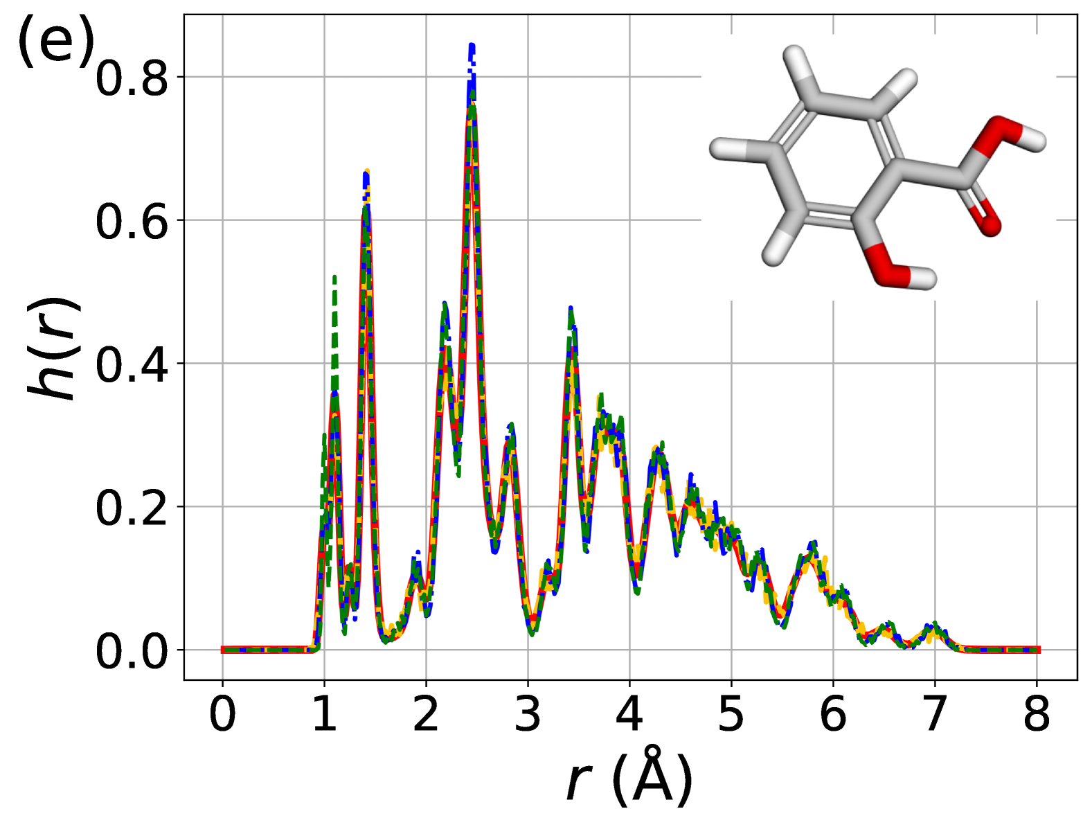
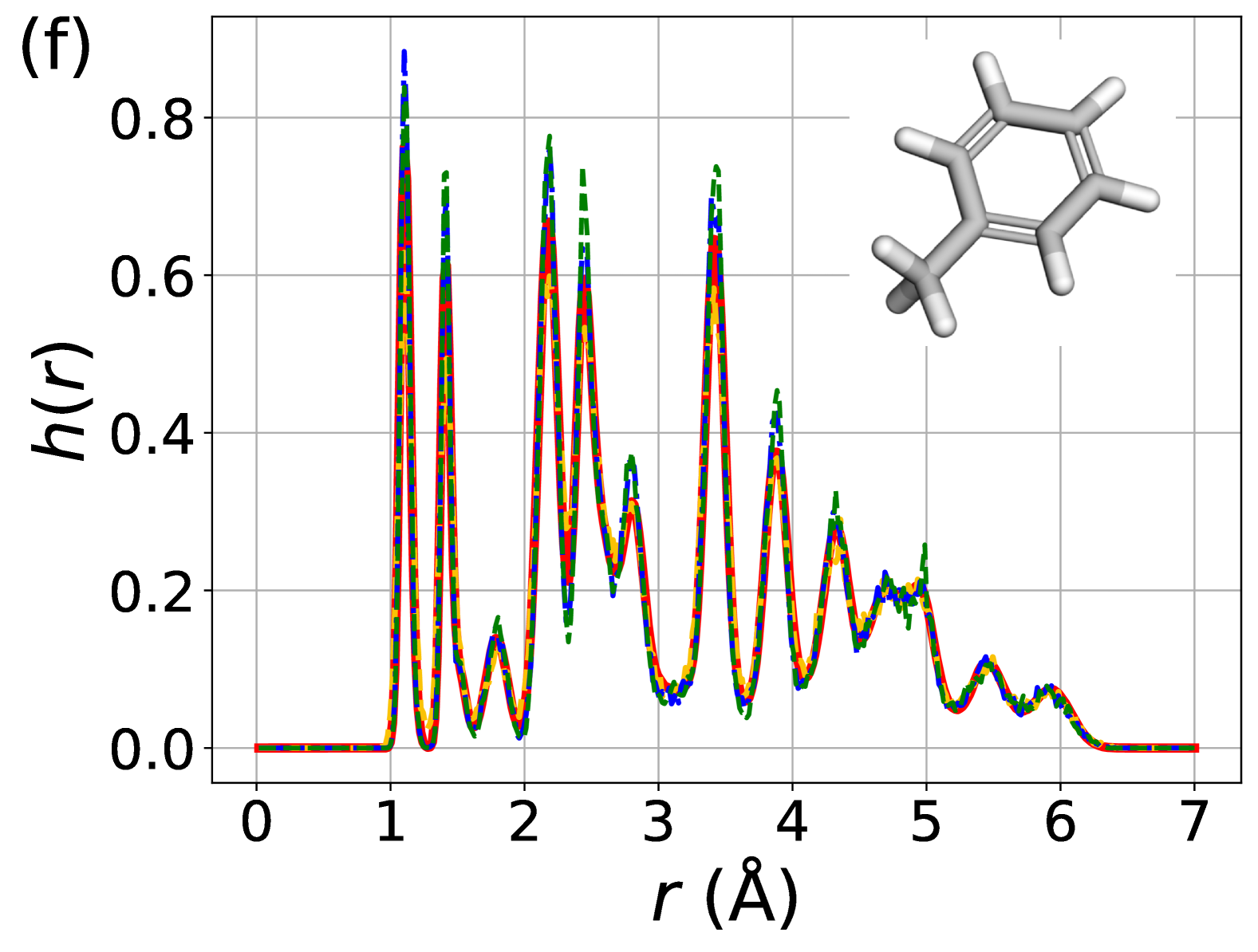
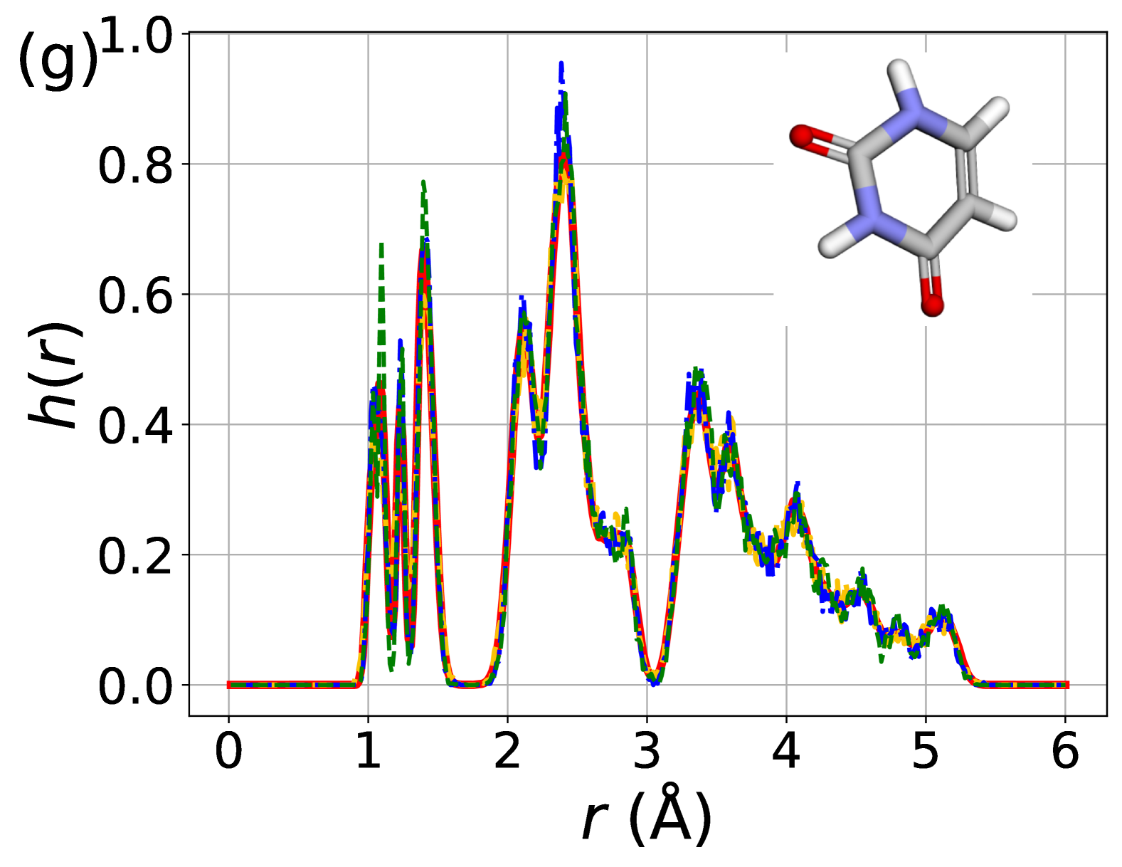
Figure 2: The distribution of interatomic distances $h(r)$ of $r($\mathrm{\SIUnitSymbolAngstrom}$)$ for (a) aspirin, (b) ethanol, (c) malonaldehyde, (d) naphthalene, (e) salicylic acid, (f) toluene, and (g) uracil in MD17 dataset. The insets display the ball-and-stick representations of these molecules learned by Piecewise method. The sample number is $1,000$.

MD17 dataset.

We first evaluate the stability of generated molecular configurations across DSM, Piecewise, and Piecewise Weighted methods, as proposed in [14]. Stability is assessed on $1,000$ samples generated at the epoch with the lowest training loss over $1,000$ epochs. All samples meet the stability criterion. With no unstable molecules in any of the sampled data, we plot the distribution of interatomic distances for these MD17 datasets, as shown in Figure 2. The figure indicates that at the peak, DSM tends to capture greater fluctuations, and PSM can more accurately learn the neighboring structure. Table 3 summarizes the mean absolute errors (MAEs) of the sampled interatomic distances and total variation distance compared to the reference molecular data. These results demonstrate that, despite the inherent bias in the training data, PSM successfully debiases molecular samples.

Table 3: Comparison of MAE of interatomic distance and Total Variation Distance (TVD) for different MD17 molecules with sample size $1,000$.

MD 17	MAE of h(r)			TVD
	DSM	Piecewise	Piecewise Weighted	DSM	Piecewise	Piecewise Weighted
Aspirin	0.1240	0.0570	0.0510	0.0662	0.0373	0.0290
Ethanol	0.1193	0.0845	0.0911	0.0663	0.0508	0.0501
Malonaldehyde	0.1003	0.0843	0.0630	0.0515	0.0492	0.0518
Naphthalene	0.1257	0.0701	0.1164	0.0716	0.0365	0.0592
Salicylic Acid	0.0799	0.0554	0.0584	0.0450	0.0424	0.0337
Toluene	0.0970	0.0769	0.0948	0.0536	0.0428	0.0490
Uracil	0.0747	0.0705	0.0560	0.0478	0.0421	0.0426

MD22 dataset.

Similarly, Figure 3 and Table 4 present $h(r)$ and the numerical metrics of the MD22 dataset, showing improved performance with the PSM method. The sample size is $128$.

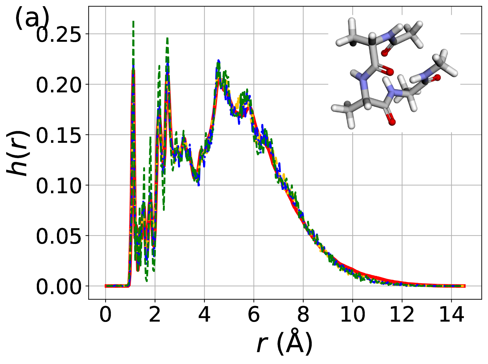
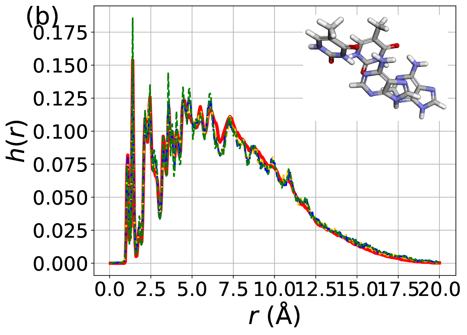
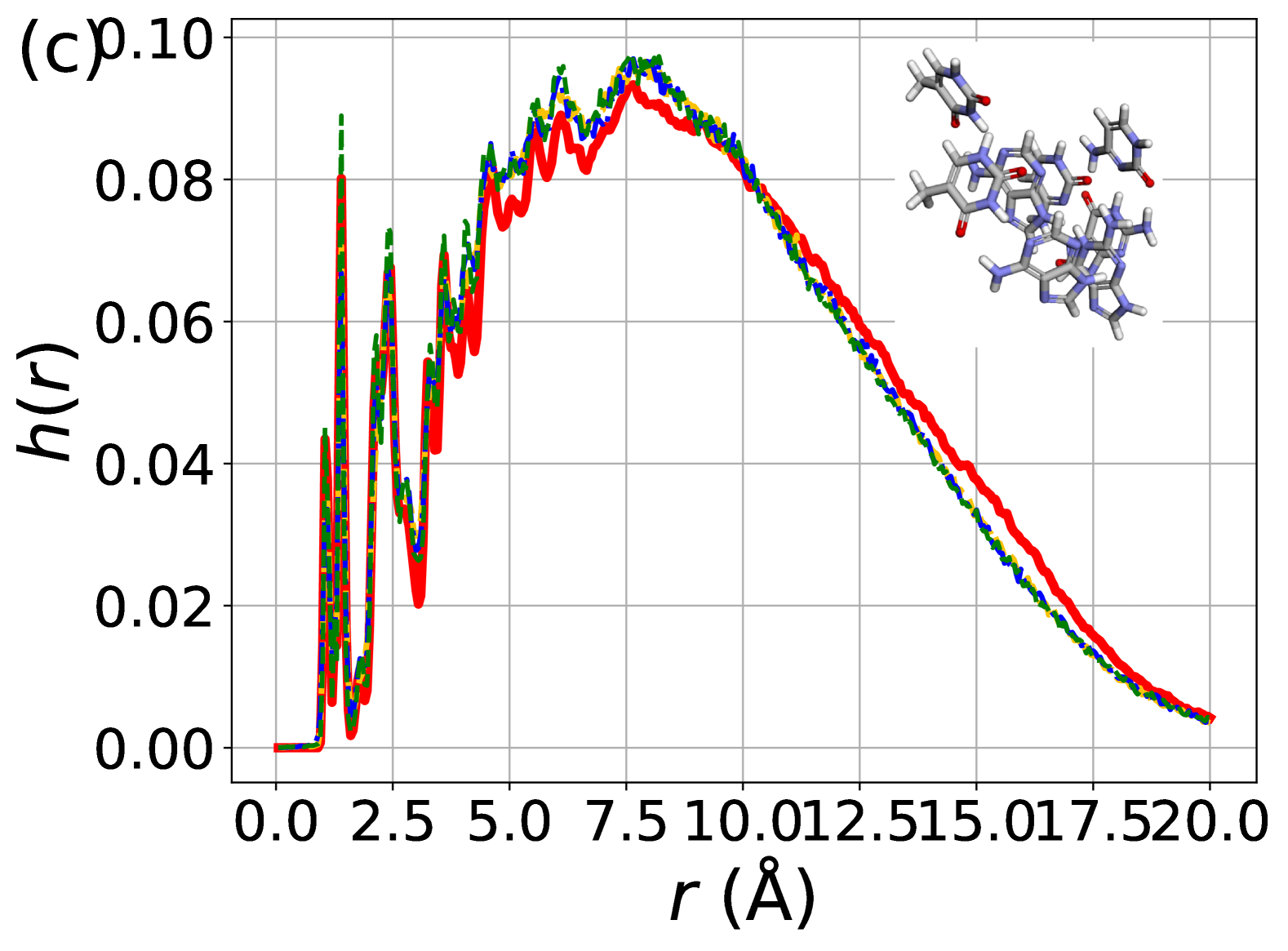
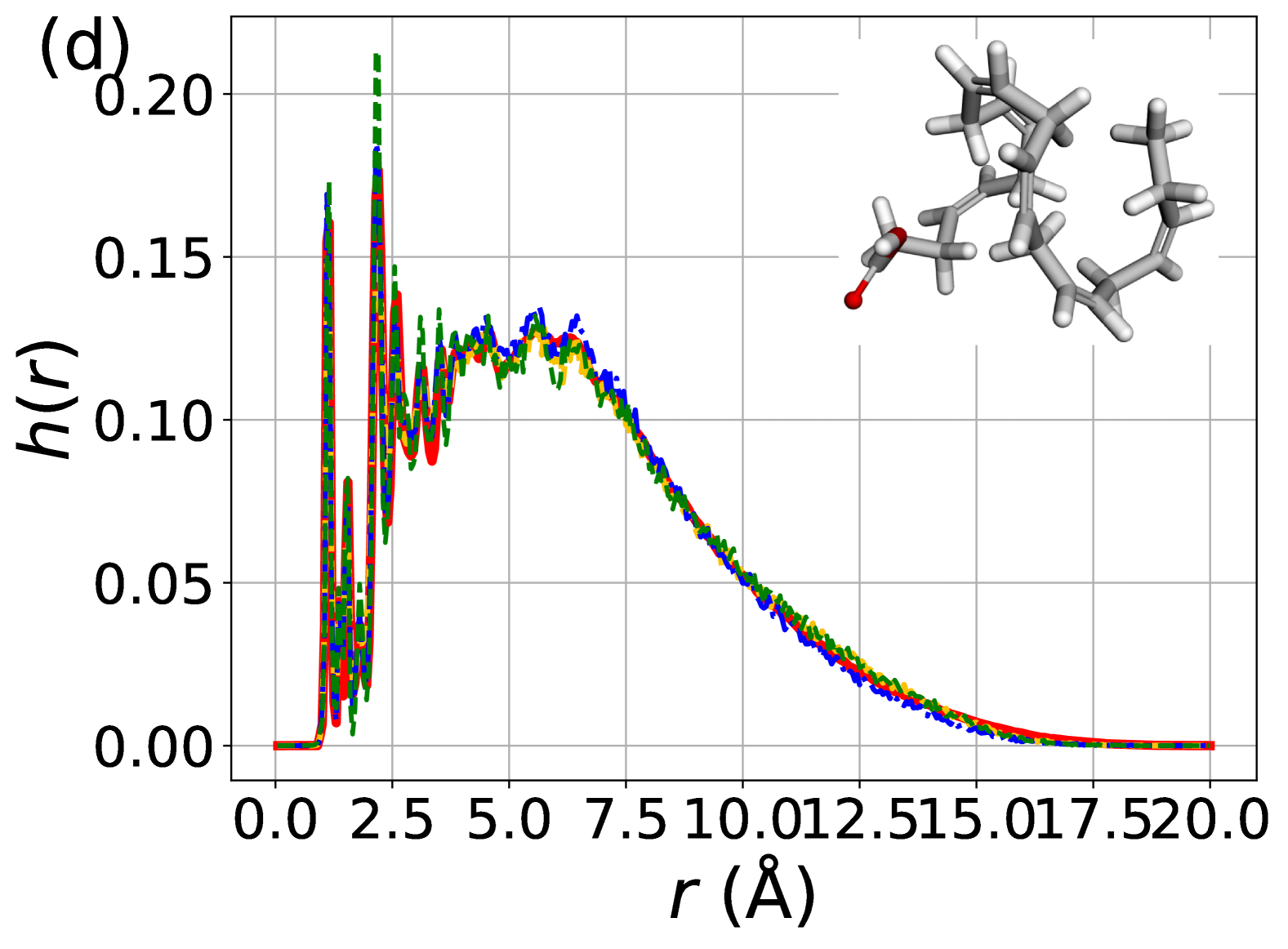
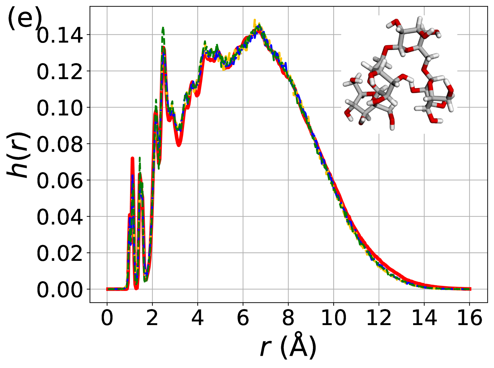
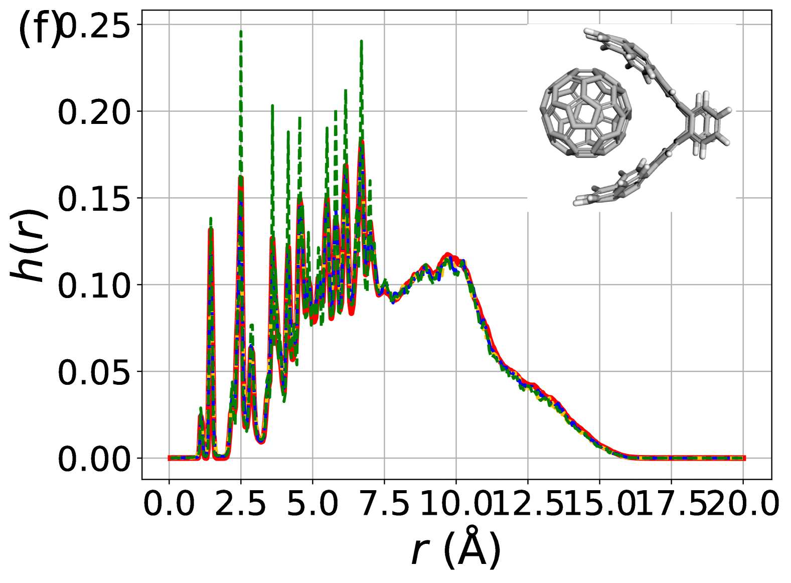
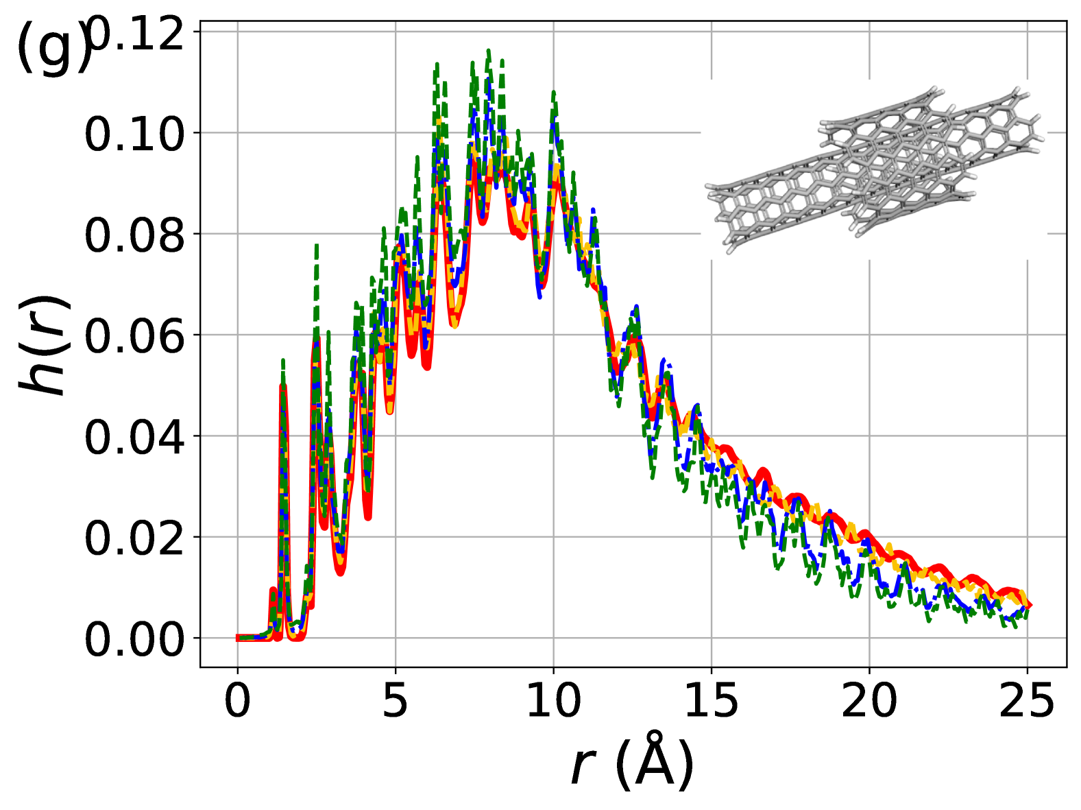
Figure 3: The distribution of interatomic distances ($r($\mathrm{\SIUnitSymbolAngstrom}$)$) for (a) Ac-Ala3-NHMe, (b) DNA base pair (AT-AT), (c) DNA base pair (AT-AT-CG-CG), (d) Docosahexaenoic acid, (e) Stachyose, (f) Buckyball catcher, (g) Dw nanotube in MD22 dataset. The insets display the ball-and-stick representations of these molecules.

Table 4: Comparison of MAE of $h(r)$ and Total Variation Distance (TVD) for different MD22 molecules.

MD 22	MAE of h(r)			TVD
	DSM	Piecewise	Piecewise Weighted	DSM	Piecewise	Piecewise Weighted
Ac-Ala3-NHMe	0.0873	0.0505	0.0486	0.0415	0.0224	0.0301
Stachyose	0.0384	0.0333	0.0424	0.0174	0.0161	0.0198
Docosahexaenoic acid	0.0602	0.0444	0.0518	0.0254	0.0221	0.0228
AT-AT	0.0767	0.0620	0.0611	0.0336	0.0292	0.0285
AT-AT-CG-CG	0.0706	0.0655	0.0677	0.0341	0.0324	0.0329
Buckyball catcher	0.0978	0.0350	0.0567	0.0417	0.0158	0.0264
Dw-nanotube	0.1527	0.0919	0.0484	0.0946	0.0597	0.0256

Debiasing conformations using SOAP descriptors.

In molecular dynamics, to illustrate that PSM extends beyond recovering ensemble averages such as $h(r)$ and achieves debiased results in terms of structural accuracy, we utilize the Smooth Overlap of Atomic Positions (SOAP) descriptor. SOAP describes the local atomic environment around a central atom $\alpha$ as a smoothly varying atomic density function:

$$\rho_{\alpha}(\mathbf{r})=\sum_{i}f_{c}(r_{i\alpha})g(r_{i\alpha})Y_{lm}(\hat{\mathbf{r}}_{i\alpha}),$$ (16)

where $r_{i\alpha}=|\mathbf{r}_{i}-\mathbf{r}_{\alpha}|$ is the distance between the central atom $\alpha$ and its neighbor $i$, and $\hat{\bm{r}}_{i\alpha}=\frac{\mathbf{r}_{i}-\mathbf{r}_{\alpha}}{r_{i\alpha}}$. The function $f_{c}(r)$ ensures locality, $g(r)$ is a radial basis function, and $Y_{lm}(\hat{\mathbf{r}})$ are spherical harmonics describing angular dependence. SOAP maintains a high-dimensional feature representation invariant under rotations. To visualize SOAP results, we apply UMAP, a nonlinear dimensionality reduction technique, for intuitive comparison.

From our ablation study (Section 4.2), we observe that the first $1,000$ frames exhibit significant biases, characterized by peak deviations. To mitigate this, we construct a training set by combining a randomly selected subset (comprising 0.5% of the total data, approximately $1,000$ frames) with the first $1,000$ frames. Training on this biased dataset, Figure 4 shows the UMAP projection of SOAP for random $1,000$ points from reference data and $1,000$ samples of PSM and DSM. The values in the figure represent the data proportions obtained by DBSCAN clustering. The results reveal that PSM produces more accurate feature weights, demonstrating that molecular features are effectively corrected through energy information.

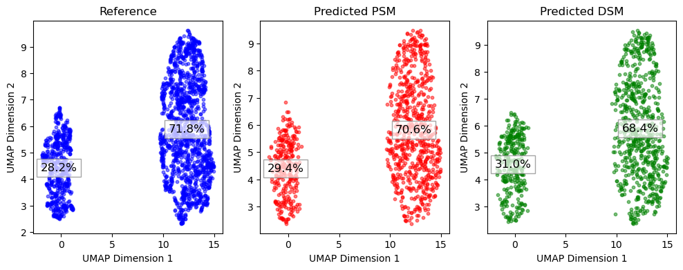
Figure 4: Umap of SOAP feature for reference data, PSM, and DSM.

4.2 Ablation Study

In this section, we investigate the impact of biased versus unbiased training data on the performance of DSM and PSM. To emphasize the effect of debiasing, we conduct experiments on both biased and unbiased datasets. Specifically, we use two different training sets: (1) a biased dataset consisting of the first $1,000$ frames of the trajectory, and (2) an unbiased dataset created by randomly selecting 10% of the reference data. Figure 5 (a) confirms that these datasets exhibit distinct bias characteristics. For this study, we use the ethanol molecule as an example.

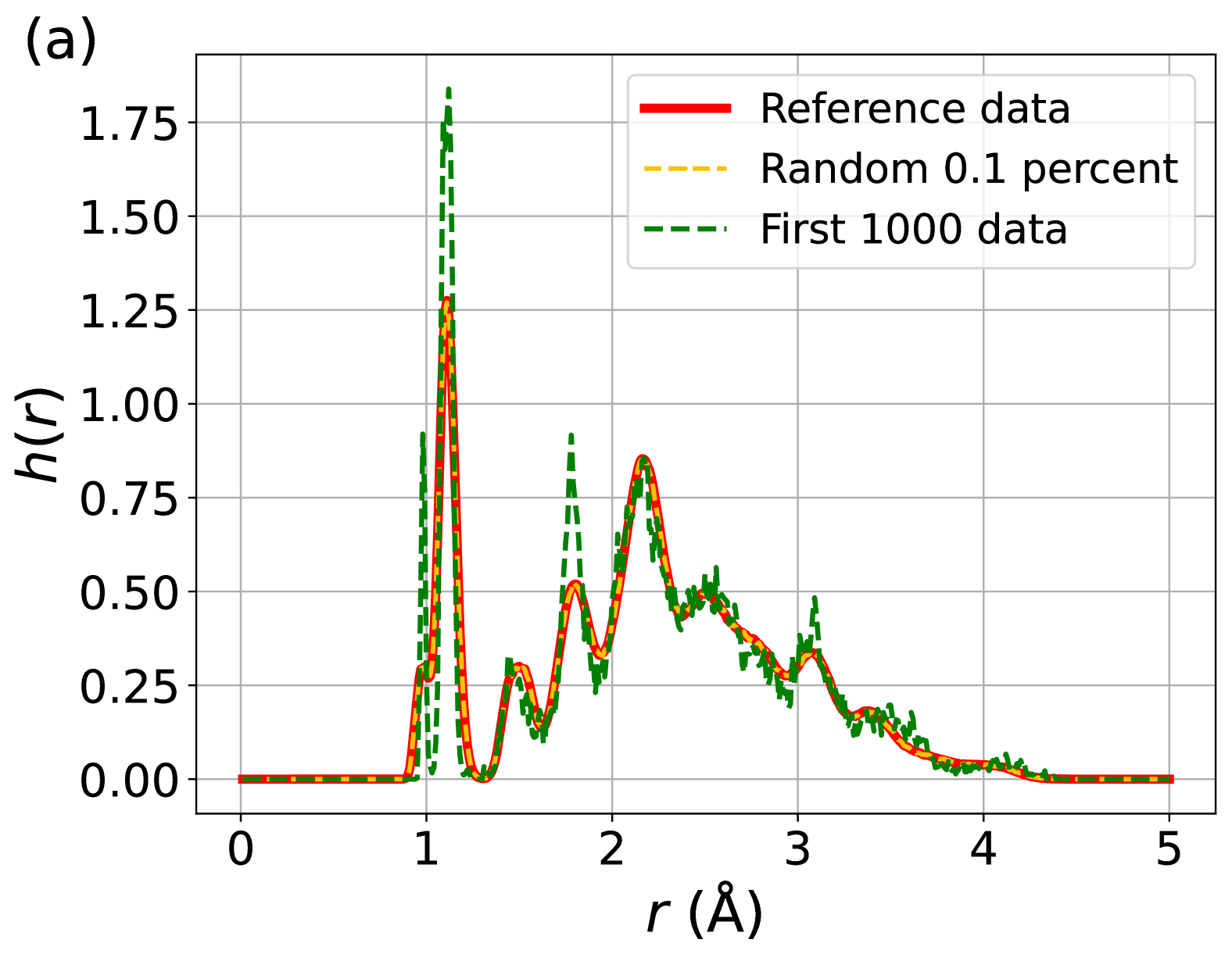
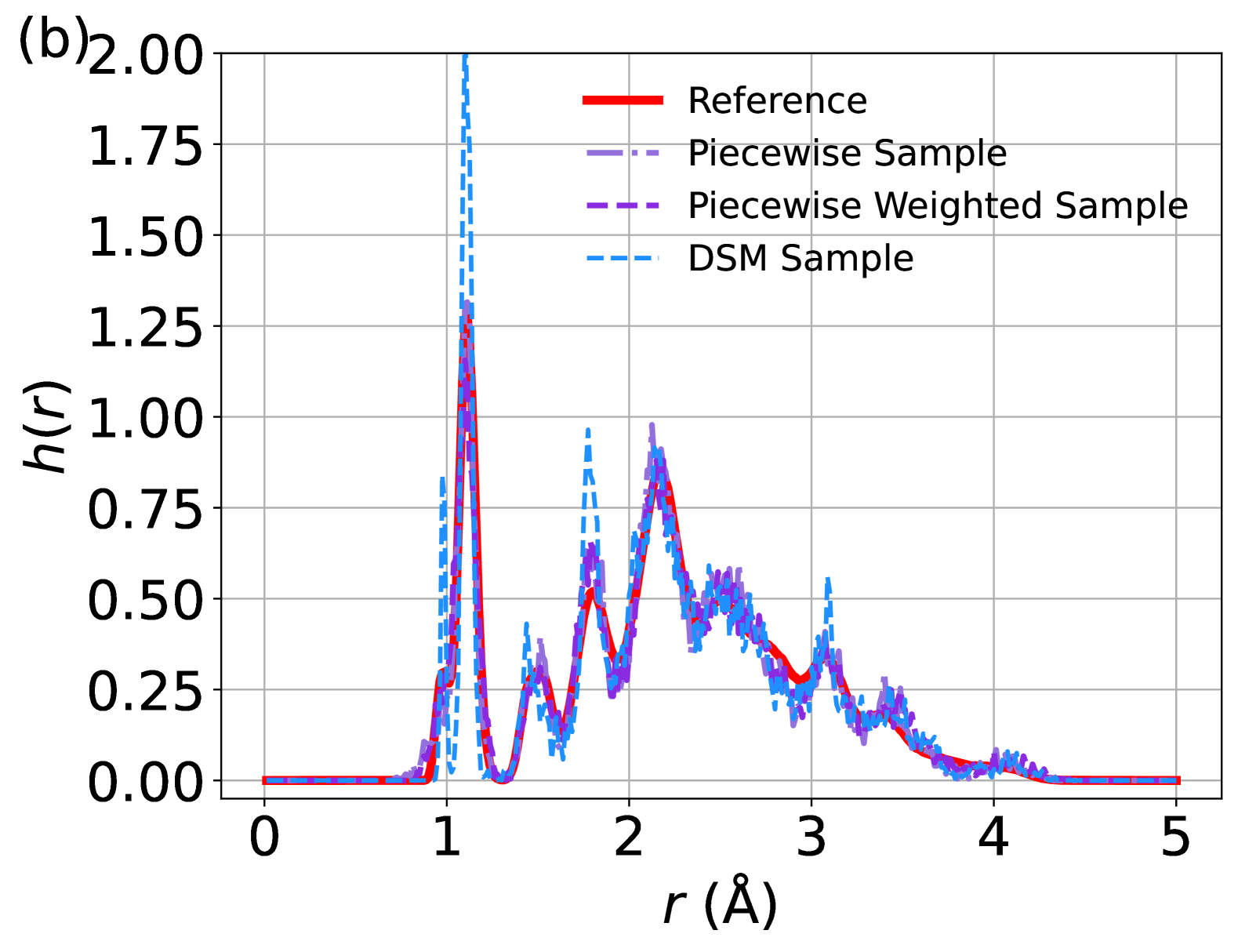
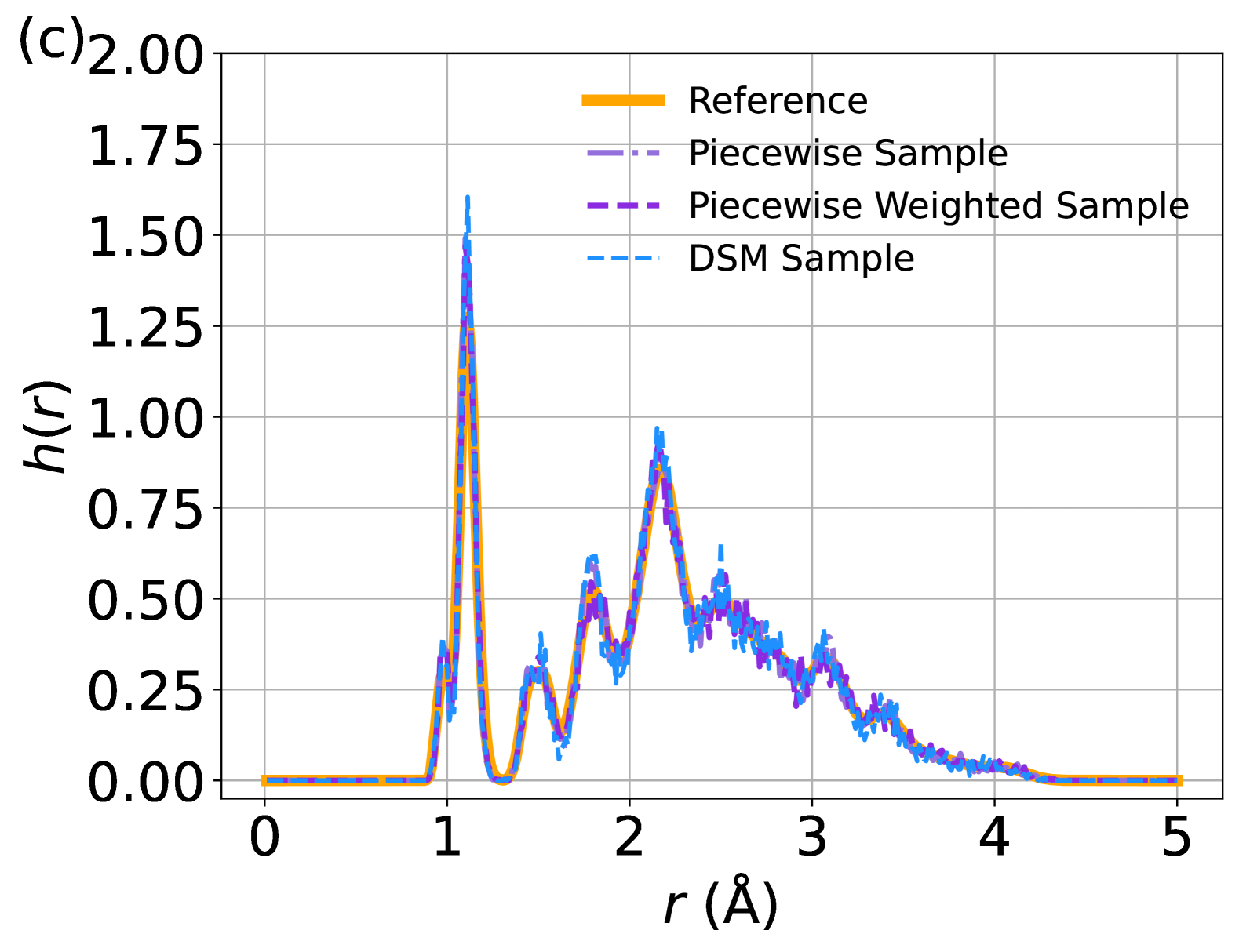
Figure 5: The distribution of interatomic distance comparisons. (a) Distribution of interatomic distances in the reference dataset, the randomly selected subset, and the first $1,000$ frames. (b) Comparison of DSM, Piecewise, and Piecewise Weighted methods trained on the first $1,000$ frames. (c) Comparison of the three methods when trained on a randomly selected 10% subset of the reference data.

Figure 5 (b) compares the sample distributions generated by DSM and PSM when trained on the first 1,000 frames. The results show that DSM mainly reflects the characteristics of the biased training data, whereas PSM successfully corrects the bias, producing samples that better align with the unbiased distribution. In contrast, Figure 5 (c) demonstrates that when the training data is initially unbiased, both DSM and PSM yield accurate estimates. These findings underscore the importance of data quality in DSM training and highlight PSM’s capability to generating samples that more accurately approximate the Boltzmann distribution.

5 Conclusions

In this study, we introduce Potential Score Matching (PSM), a method designed to mitigate biases in non-Boltzmann distributions by incorporating force labels. Traditional molecular dynamics simulations are computationally expensive. While diffusion models offer an alternative by learning a score function to generate samples that satisfy the training data distribution, obtaining training data that accurately follows the Boltzmann distribution is challenging. PSM relaxes these constraints. Theoretical analysis indicates that PSM provides training with lower variance and more accurate score estimations in the vicinity of $t=0$, which allows for a concentrated training effort around this point. This has led to the development of two novel loss formulations: Piecewise and Piecewise Weighted losses. Empirical assessments validate the performance of PSM over Denoising Score Matching by effectively debiasing data towards the Boltzmann distribution. Furthermore, our research extends the application of PSM to high-dimensional real-world datasets, such as MD22 and MD17, demonstrating its capability in handling complex molecular modeling challenges.

Additionally, flow matching has proven to be an effective method for generating molecular conformations and predicting properties [23, 5, 27]. Progress in this area [37, 10] has resulted in unified frameworks that integrate diffusion models and flow matching techniques. Considering the established relation between the velocity field and the score function, as expressed by $v(\bm{x},t)=\frac{\dot{\alpha}_{t}}{\alpha_{t}}\bm{x}+\gamma_{t}\left(\frac{\dot{\alpha}_{t}}{\alpha_{t}}\gamma_{t}-\dot{\gamma}_{t}\right)s(\bm{x},t)$, where $\bm{x}_{t}=\alpha_{t}\bm{y}_{1}+\gamma_{t}\bm{y}_{0}=\alpha_{t}\bm{x}_{0}+\gamma_{t}\varepsilon$, and $\bm{y}_{0}$, $\bm{y}_{1}$ are sampled from the noise and data distributions respectively, our PSM framework is well-positioned for extension to flow matching. This prospective expansion is earmarked for future exploration, while further theoretical insights and formulations for VPSDE and VESDE are delineated in Appendix D.

Appendix A Preliminary

A.1 Diffusion Models

A diffusion model typically consists of a forward noise addition process and a reverse denoising process. In the forward process, noise is iteratively added to the data $\bm{x}$ (at $t=0$), gradually transforming the distribution into an approximation of a Gaussian distribution at time $T$, independent of the initial state $\bm{x}_{0}$. The reverse process then generates samples that conform to the data distribution by leveraging information obtained from the forward process.

We introduce the Variance-Preserving Stochastic Differential Equation (VPSDE) and the Variance-Exploding Stochastic Differential Equation (VESDE) [33], summarized in the following Table 5. Here, $\mathbf{z}$ is a random noise, $i\in\{1,\cdots,N\}$ is one of noising steps.

Table 5: VESDE and VPSDE.

	VESDE	VPSDE
Noise addition	$\mathbf{x}_{i}=\mathbf{x}_{i-1}+\sqrt{\sigma_{i}^{2}-\sigma_{i-1}^{2}}\mathbf{z}_{i-1}$	$\mathbf{x}_{i}=\alpha_{i}\mathbf{x}_{0}+\sigma_{i}\mathbf{z}_{i}$
SDE Formulation	$\mathrm{d}\mathbf{x}_{t}=\sigma(t)\mathrm{d}W_{t}$	$\mathrm{d}\mathbf{x}_{t}=-\frac{1}{2}\beta_{t}\mathbf{x}_{t}\mathrm{d}t+\sqrt{\beta_{t}}\mathrm{d}W_{t}$
Parameterization	$\sigma(t)=\sigma_{\min}(\sigma_{\max}/\sigma_{\min})^{t}$	$\beta_{t}=\beta_{\min}+(\beta_{\max}-\beta_{\min})t$
Transition Distribution	$\mathcal{N}\left(\bm{x}_{t};\bm{x}_{0},\sigma_{\min}^{2}(\sigma_{\max}/\sigma_{\min})^{2t}\mathbf{I}\right)$	$\mathcal{N}\left(\bm{x}_{t};\bm{x}_{0}e^{-\frac{1}{2}\int_{0}^{t}\beta_{s}ds},(1-e^{-\int_{0}^{t}\beta_{s}ds})\bm{I}\right)$

We sample from the diffusion model follows a Predictor-Corrector (PC) scheme. The predictor step follows the time-reversed SDE, while the corrector step applies Langevin dynamics to refine the sample. Given a time step $\Delta t$, the predictor step updates the sample as:

$$\tilde{\mathbf{x}}_{t-\Delta t}=\mathbf{x}_{t}-f(\mathbf{x}_{t},t)\Delta t+g(t)\sqrt{\Delta t}\mathbf{z}_{t},$$ (17)

where $\mathbf{z}_{t}\sim\mathcal{N}(\mathbf{0},\mathbf{I})$ is Gaussian noise, and $f$ and $g$ are drift and diffusion coefficients. The corrector step refines $\tilde{\mathbf{x}}_{t-\Delta t}$ using Langevin dynamics $\mathbf{x}_{t-\Delta t}=\tilde{\mathbf{x}}_{t-\Delta t}+\eta\nabla_{\mathbf{x}}\log p_{t}(\mathbf{x})+\sqrt{2\eta}\mathbf{z}^{\prime}$, where $\eta$ is the step size, and $\mathbf{z}^{\prime}\sim\mathcal{N}(\mathbf{0},\mathbf{I})$. This two-step process improves the quality of generated samples and enhances convergence to the data distribution.

A.2 Equiformer-v2

A.2.1 Equivariance and Irreducible Repressentation

In molecular systems, molecular structures are typically represented as graph, where atomic coordinates, atomic numbers, and bonded connections define a molecular graph. Ensuring properties such as symmetry and equivariance in these graph representations is crucial for capturing molecular interactions accurately.

Graph representation.

A molecular graph is defined as $G=(V,E)$, where $V=\{v_{1},v_{2},\dots,v_{|V|}\}$ represents the set of atoms (nodes), and $E=\{e_{ij}\mid(i,j)\subset V\times V\}$ denotes the set of edges capturing atomic interactions. The number of atoms in a molecule is denoted as $N=|V|$. Each node $v_{i}\in V$ is characterized by its nuclear charge $z_{i}$ and 3D coordinate $r_{i}\in\mathbb{R}^{3}$. Our goal is to design a generative model that learns to generate molecular distributions while preserving the underlying chemical and spatial properties.

Graph neural networks.

Graph Neural Networks (GNNs) are widely used to process graph-structured data by propagating information across nodes and edges. At each iteration $t$, node features $\mathbf{h}_{v}^{(t)}$ are updated using a message-passing mechanism:

$$\mathbf{m}_{v}^{(t+1)}=\sum_{u\in\mathcal{N}(v)}\phi(\mathbf{h}_{v}^{(t)},\mathbf{h}_{u}^{(t)},\mathbf{e}_{vu}),\quad\mathbf{h}_{v}^{(t+1)}=\psi(\mathbf{h}_{v}^{(t)},\mathbf{m}_{v}^{(t+1)}),$$ (18)

where $\mathcal{N}(v)$ represents the neighboring nodes of $v$, $\mathbf{e}_{vu}$ denotes the edge feature between nodes $v$ and $u$, and $\phi(\cdot)$ and $\psi(\cdot)$ are learnable functions, implemented as networks.

Equivariance and irreducible representations.

Equivariance serves as a fundamental property in neural networks, providing strong prior knowledge that enhances data efficiency in molecular modeling. A function $f:X\to Y$ is equivariant under a transformation group $G$ if, for any input $x\in X$, output $y\in Y$, and group element $g\in G$, $f\left(D_{X}(g)x\right)=D_{Y}(g)f(x)$ holds, where $D_{X}(g)$ and $D_{Y}(g)$ are transformation matrices parameterized by $g$ in $X$ and $Y$. In 3D atomistic graphs, molecular structures must maintain equivariance under the Euclidean group $E(3)$, which includes translations, rotations, and reflections.

For the Euclidean group $E(3)$, scalar quantities remain invariant under rotations, whereas vector quantities transform accordingly. To enforce translation symmetry, computations are performed on relative positions. Since rotation and inversion transformations commute, any representation of the special orthogonal group $SO(3)$ can be decomposed into irreducible representations (irreps), which serve as fundamental transformation components. Equivariant neural networks leverage these irreducible representations to construct features that remain equivariant to 3D rotations.

For probabilistic models, the equivariance property extends to probability distributions. A probability distribution $p(\bm{x}_{t})$ is equivariant under the special Euclidean group $SE(3)$ if, for any transformation $T_{g}$ corresponding to $g\in SE(3)$, then $p(\bm{x}_{t})=p(T_{g}(\bm{x}_{t}))$, and $p(\bm{x}_{t-1}\mid\bm{x}_{t})=p(T_{g}(\bm{x}_{t-1})\mid T_{g}(\bm{x}_{t}))$. A similar definition applies for $E(3)$.

A.2.2 Equiformer-v2 Network

In our research, we harness the capabilities of the Equiformer-v2 network [22] to maintain $SE(3)$/$E(3)$-equivariance, a critical aspect for accurately modeling molecular configurations. This advanced architecture builds on the principles of irreducible representations, ensuring that its operations and features are equivariant and robust. Other works have also incorporated designs ensuring molecular invariance and equivariance [40, 31, 21, 28].

Building upon the Equiformer, the Equiformer-v2 introduces sophisticated equivariant graph attention mechanisms, supplanting standard Transformer operations with their SE(3)/E(3)-equivariant counterparts and utilizing tensor products for higher-degree representations. Node embeddings are crafted by concatenating channel-dimension features and applying rotations based on relative positions or edge orientations.

To enhance computational efficiency, Equiformer-v2 forgoes separate depth-wise tensor products and linear layers in favor of a single SO(2) linear layer that processes scalar and irreps features distinctly. It encodes edge distance information using radial basis functions, integrating them into the node embeddings.

The attention mechanisms benefit from extra normalization and separable $S^{2}$ activation for improved stability. The network’s feed-forward section employs a two-layer MLP with SiLU activation. The output head either aggregates scalar predictions or computes atom-wise forces, utilizing equivariant graph attention to boost expressiveness and scalability.

ESCN convolution.

The ESCN convolution refines equivariant tensor products by substituting conventional SO(3) operations with SO(2) linear ones. Typically, SO(3) convolutions combine input irreps features with spherical harmonics of relative positions using Clebsch-Gordan coefficients. ESCN simplifies this by aligning the relative position vector with a fixed axis through rotation, reducing dependencies and limiting interactions to cases where $m_{f}=0$, which streamlines computations while preserving equivariance.

Attention re-normalization.

To maintain stability at higher $L_{\text{max}}$, we introduce an additional layer normalization step before non-linear transformations, ensuring well-scaled scalar features $f_{ij}^{(0)}$. Attention weights are computed through a leaky ReLU and a linear layer, promoting numerical stability in operations like softmax, which aids in training convergence and model robustness.

Separable $S^{2}$ activation

The separable $S^{2}$ activation processes degree-0 and higher-degree features separately. Degree-0 vectors are partially activated with SiLU, while the remainder is blended with higher-degree vectors for $S^{2}$ activation. This selective processing minimizes cross-degree interference, stabilizes gradients, and enhances expressiveness, particularly in FFNs.

Separable layer normalization.

Separable layer normalization (SLN) extends traditional equivariant normalization by independently normalizing degree-0 and higher-degree features. By computing their means and standard deviations separately, SLN preserves inter-degree dynamics, enhancing stability and expressiveness, especially in high $L_{\text{max}}$ scenarios.

Our network architecture is predicated on Equiformer-v2, which yields both one-dimensional energy and three-dimensional force terms. For the $\epsilon$-net output, we utilize only the energy head. Furthermore, we adapt the model to consider time as an additional input feature to align with the diffusion model’s time-dependent noise addition.

Appendix B Derivation of Loss Function

B.1 Proof of Theorem 1

Proof.

Assume that $p(\bm{x}_{0})\propto e^{-\mathcal{E}/(k_{B}T)}$, the derivation of the loss function follows from the transformation of scores using the Gaussian transition probability density function and the integration by parts. Since $\nabla_{\bm{x}_{t}}p(\bm{x}_{t}|\bm{x}_{0})=\frac{1}{\alpha_{t}}\nabla_{\bm{x}_{0}}p(\bm{x}_{t}|\bm{x}_{0})$,

$$\nabla_{\bm{x}_{t}}\log p(\bm{x}_{t}) =\frac{\nabla_{\bm{x}_{t}}\int p(\bm{x}_{0})p(\bm{x}_{t}|\bm{x}_{0})d\bm{x}_{0}}{p(\bm{x}_{t})}=\frac{\int p(\bm{x}_{0})\nabla_{\bm{x}_{t}}\left(e^{-\frac{\|\bm{x}_{t}-\alpha_{t}\bm{x}_{0}\|^{2}}{2\sigma_{t}^{2}}}\right)d\bm{x}_{0}}{p(\bm{x}_{t})}$$ (19)

$$=\frac{\int p(\bm{x}_{0})\left(-\frac{1}{\alpha_{t}}\nabla_{\bm{x}_{0}}e^{-\frac{\|\bm{x}_{t}-\alpha_{t}\bm{x}_{0}\|^{2}}{2\sigma_{t}^{2}}}\right)d\bm{x}_{0}}{p(\bm{x}_{t})}=\frac{\int\frac{1}{\alpha_{t}}\left(\nabla_{\bm{x}_{0}}p(\bm{x}_{0})\right)e^{-\frac{\|\bm{x}_{t}-\alpha_{t}\bm{x}_{0}\|^{2}}{2\sigma_{t}^{2}}}d\bm{x}_{0}}{p(\bm{x}_{t})}$$

$$=\int\frac{1}{\alpha_{t}}\left(p(\bm{x}_{0})\nabla_{\bm{x}_{0}}\log p(\bm{x}_{0})\right)\frac{1}{p(\bm{x}_{t})}e^{-\frac{\|\bm{x}_{t}-\alpha_{t}\bm{x}_{0}\|^{2}}{2\sigma_{t}^{2}}}d\bm{x}_{0}$$

$$=\int\frac{1}{\alpha_{t}}p(\bm{x}_{0}|\bm{x}_{t})\nabla_{\bm{x}_{0}}\log p(\bm{x}_{0})d\bm{x}_{0}$$

$$=\frac{1}{\alpha_{t}}\mathbb{E}_{\bm{x}_{0}|\bm{x}_{t}}\left[\frac{-\nabla_{\bm{x}_{0}}\mathcal{E}}{k_{B}T}\right]=\frac{1}{\alpha_{t}}\mathbb{E}_{\bm{x}_{0}|\bm{x}_{t}}\left[\frac{\bm{F}}{k_{B}T}\right]\,,$$

where $\mathcal{E}$ is the energy function, and $\bm{F}$ represents the force derived from $-\nabla_{\bm{x}_{0}}\mathcal{E}$. Specifically, for the VESDE, $\alpha_{t}=1$, then $\nabla_{\bm{x}_{t}}\log p(\bm{x}_{t})=\mathbb{E}_{\bm{x}_{0}|\bm{x}_{t}}\left[-\frac{\nabla_{\bm{x}_{0}}\mathcal{E}}{k_{B}T}\right]\,.$

For simplicity, let $k_{B}T=1$. Combining these results, the potential score matching loss can be derived as:

$$\mathcal{L}_{\text{score - model}} =\mathbb{E}_{t\sim U(0,1)}\mathbb{E}_{\bm{x}_{t}\sim p(\bm{x}_{t}|\bm{x}_{0})}\mathbb{E}_{\bm{x}_{0}}\|s_{\theta}(\bm{x}_{t},t)-(-\frac{1}{\alpha_{t}}\nabla_{\bm{x}_{0}}\mathcal{E})\|^{2}$$ (20)

$$=\mathbb{E}_{t\sim U(0,1)}\mathbb{E}_{\bm{x}_{t}\sim p(\bm{x}_{t}|\bm{x}_{0})}\mathbb{E}_{\bm{x}_{0}}\|s_{\theta}(\bm{x}_{t},t)-\frac{1}{\alpha_{t}}\bm{F}\|^{2}.$$ (21)

∎

The reason why $\nabla_{\bm{x}_{t}}\log p(\bm{x}_{t})=\mathbb{E}_{\bm{x}_{0}|\bm{x}_{t}}\left[-\nabla_{\bm{x}_{0}}\mathcal{E}\right]$ (objective (19)) is the solution of the loss function ((20)) lies in Theorem 3. According to the above expansion, label $\nabla_{\bm{x}_{t}}\log p(\bm{x}_{t})$ can be rewritten as

$$\nabla_{\bm{x}_{t}}\log p(\bm{x}_{t}) =\frac{\nabla_{\bm{x}_{t}}\int p(\bm{x}_{0})p(\bm{x}_{t}|\bm{x}_{0})d\bm{x}_{0}}{p(\bm{x}_{t})}=\frac{\int p(\bm{x}_{0})(-\frac{\bm{x}_{t}-\bm{x}_{0}}{\sigma_{t}^{2}})p(\bm{x}_{t}|\bm{x}_{0})d\bm{x}_{0}}{p(\bm{x}_{t})}$$ (22)

$$=\int p(\bm{x}_{0}|\bm{x}_{t})(-\frac{\bm{x}_{t}-\bm{x}_{0}}{\sigma_{t}^{2}})d\bm{x}_{0}=\mathbb{E}_{\bm{x}_{0}|\bm{x}_{t}}\left[\frac{\bm{x}_{0}-\bm{x}_{t}}{\sigma_{t}^{2}}\right]\,,$$

which is consistent with the writing of $``\bm{x}_{0}$-model$"$. Similarly, we can rewrite the loss function with a network representing $\bm{x}_{0}$.

$$\mathbb{E}_{\bm{x}_{0}|\bm{x}_{t}}\left[\frac{\bm{x}_{0}-\bm{x}_{t}}{\sigma_{t}^{2}}+\nabla_{\bm{x}_{0}}\mathcal{E}(\bm{x}_{0})\right]=\mathbb{E}_{\bm{x}_{0}|\bm{x}_{t}}\left[\frac{\bm{x}_{0}-\bm{x}_{t}+\sigma_{t}^{2}\nabla_{\bm{x}_{0}}\mathcal{E}(\bm{x}_{0})}{\sigma_{t}^{2}}\right]=\mathbb{E}_{\bm{x}_{0}|\bm{x}_{t}}\left[\frac{\bm{x}_{0}-\mathcal{D}_{\theta}}{\sigma_{t}^{2}}\right]\,.$$ (23)

$$\mathcal{L}_{\bm{x}_{0}-\text{model}}=\mathbb{E}_{t\sim U(0,1)}\mathbb{E}_{\bm{x}_{t}\sim p(\bm{x}_{t}|\bm{x}_{0})}\mathbb{E}_{\bm{x}_{0}}\|\mathcal{D}_{\theta}-\bm{x}_{t}-\sigma_{t}^{2}\nabla_{\bm{x}_{0}}\mathcal{E}(\bm{x}_{0})\|_{2}^{2}\,.$$ (24)

Theorem 3.

Let $X$ be an integrable random variable. Then for each $\sigma$-algebra $\mathcal{V}$ and $Y\in\mathcal{V}$, $Z=\mathbb{E}(X|\mathcal{V})$ solves the least square problem [12]

$$\|Z-X\|=\min_{Y\in\mathcal{V}}\|Y-X\|\,,$$

where $\|Y\|=\left(\int Y^{2}dP\right)^{\frac{1}{2}}$.

To prove the theorem, we first introduce a lemma.

Lemma 1.

If $Y$ is $\mathcal{V}$-measurable, and $f$ is a measurable function in the sense that its domain and codomain are appropriately aligned with the $\sigma$-algebras, then $f(Y)$ will also be $\mathcal{V}$-measurable [13].

Proof of Lemma 1.

Let $Y$ be a $\mathcal{V}$-measurable random variable, and let $f$ be a measurable function with an appropriate domain and codomain aligned with the $\sigma$-algebras. We need to show that $f(Y)$ is also $\mathcal{V}$-measurable.

Recall the definition of a measurable function: A function $f:\Omega_{1}\to\Omega_{2}$ is measurable with respect to the $\sigma$-algebras $\mathcal{A}_{1}$ and $\mathcal{A}_{2}$ if for any $B\in\mathcal{A}_{2}$, the preimage of $B$ under $f$, denoted by $f^{-1}(B)$, belongs to $\mathcal{A}_{1}$.

Now, let $B\in\mathcal{B}$, where $\mathcal{B}$ is the $\sigma$-algebra associated with the codomain of $f$. The object is to show that $f^{-1}(B)\in\mathcal{V}$ for any $B\in\mathcal{B}$.

Since $f$ is a measurable function, we have $f^{-1}(B)\in\mathcal{A}_{1}$ for any $B\in\mathcal{B}$. Here, $\mathcal{A}_{1}$ is the $\sigma$-algebra associated with the domain of $f$. Now, consider the random variable $Y:\Omega\to\Omega_{1}$, where $\Omega$ is the sample space. Since $Y$ is $\mathcal{V}$-measurable, we have $Y^{-1}(A)\in\mathcal{V}$ for any $A\in\mathcal{A}_{1}$.

Now, we want to find the preimage of $B$ under the composition of $f$ and $Y$, i.e., $(f\circ Y)^{-1}(B)$. By the properties of inverse functions, we have:

$$(f\circ Y)^{-1}(B)=Y^{-1}(f^{-1}(B))$$

We know that $f^{-1}(B)\in\mathcal{A}_{1}$, so $Y^{-1}(f^{-1}(B))\in\mathcal{V}$ because $Y$ is $\mathcal{V}$-measurable. This implies that the composition of $f$ and $Y$, denoted by $f(Y)$, is also $\mathcal{V}$-measurable.

Proof of Theorem 3.

Let $X$ be an integrable random variable, $\mathcal{V}$ be a $\sigma$-algebra, and $Y\in\mathcal{V}$. We need to show that $Z=\mathbb{E}(X|\mathcal{V})$ minimizes the least square problem $|Z-X|=\min_{Y\in\mathcal{V}}|Y-X|$.

First, recall the property of conditional expectation: $\mathbb{E}(Z|\mathcal{V})=Z$ for any $Z\in\mathcal{V}$. Consider the difference $X-Y$ for any $Y\in\mathcal{V}$. We can write this difference as:

$$X-Y=(X-\mathbb{E}(X|\mathcal{V}))+(\mathbb{E}(X|\mathcal{V})-Y)$$

Note that $\mathbb{E}(X|\mathcal{V})\in\mathcal{V}$, so the second term $(\mathbb{E}(X|\mathcal{V})-Y)\in\mathcal{V}$. Using the property of conditional expectation, we have $\mathbb{E}(\mathbb{E}(X|\mathcal{V})-Y|\mathcal{V})=\mathbb{E}(X|\mathcal{V})-Y$.

Now, let’s calculate the conditional expectation of the product of $(X-\mathbb{E}(X|\mathcal{V}))$ and $(\mathbb{E}(X|\mathcal{V})-Y)$:

$$\mathbb{E}((X-\mathbb{E}(X|\mathcal{V}))(\mathbb{E}(X|\mathcal{V})-Y)|\mathcal{V})=\mathbb{E}((X-\mathbb{E}(X|\mathcal{V}))(\mathbb{E}(X|\mathcal{V})-Y))=0$$

The last equality follows from the fact that the product of the two terms is uncorrelated, and their expectation is zero. This implies that $(X-\mathbb{E}(X|\mathcal{V}))$ and $(\mathbb{E}(X|\mathcal{V})-Y)$ are orthogonal.

Now, we can use the Pythagorean theorem for Hilbert spaces:

$$|X-Y|^{2}=|X-\mathbb{E}(X|\mathcal{V})|^{2}+|\mathbb{E}(X|\mathcal{V})-Y|^{2}$$

Notice that the right-hand side is minimized when $|\mathbb{E}(X|\mathcal{V})-Y|^{2}$ is minimized. This is true because $|X-\mathbb{E}(X|\mathcal{V})|^{2}$ is constant and non-negative. Therefore, the least square problem is minimized when $Y=\mathbb{E}(X|\mathcal{V})$, i.e., $Z=\mathbb{E}(X|\mathcal{V})$.

Hence, we have proved that $Z=\mathbb{E}(X|\mathcal{V})$ solves the least square problem:

$$|Z-X|=\min_{Y\in\mathcal{V}}|Y-X|\,.$$

B.2 Proof of Theorem 2

Proof.

Let $I_{1}$ be the formula on the left side $\mathbb{E}_{q\left(\bm{x}_{0}\mid\bm{x}_{t}\right)}\left[\nabla\log p\left(\bm{x}_{0}\right)\right]-\mathbb{E}_{p\left(\bm{x}_{0}\mid\bm{x}_{t}\right)}\left[\nabla\log p\left(\bm{x}_{0}\right)\right]$, and $I_{2}$ be the right one, $\mathbb{E}_{q\left(\bm{x}_{0}\mid\bm{x}_{t}\right)}\left[\nabla\log q\left(\bm{x}_{0}\right)\right]-\mathbb{E}_{p\left(\bm{x}_{0}\mid\bm{x}_{t}\right)}\left[\nabla\log p\left(\bm{x}_{0}\right)\right]$.

$$I_{1} =\int\nabla\log p\left(\bm{x}_{0}\right)\left(q\left(\bm{x}_{0}\mid\bm{x}_{t}\right)-p\left(\bm{x}_{0}\mid\bm{x}_{t}\right)\right)d\bm{x}_{0}\,,$$ (25)

$$I_{2} =\int\left(\nabla\log q\left(\bm{x}_{0}\right)q\left(\bm{x}_{0}\mid\bm{x}_{t}\right)-\nabla\log p\left(\bm{x}_{0}\right)p\left(\bm{x}_{0}\mid\bm{x}_{t}\right)\right)d\bm{x}_{0}\,,$$

$$I_{3} =\int\left(\nabla\log q\left(\bm{x}_{0}\right)-\nabla\log p\left(\bm{x}_{0}\right)\right)q\left(\bm{x}_{0}\mid\bm{x}_{t}\right)d\bm{x}_{0}\,.$$

Then $I_{2}=I_{1}+I_{3}$. We only need to prove that for $t$ near $0$,

$$\left\|I_{1}\right\|_{2}^{2}= \left\|\int\nabla\log p\left(\bm{x}_{0}\right)\left(q\left(\bm{x}_{0}\mid\bm{x}_{t}\right)-p\left(\bm{x}_{0}\mid\bm{x}_{t}\right)\right)d\bm{x}_{0}\right\|_{2}^{2}$$ (26)

$$\leqslant\left\|\int\left(\nabla\log q\left(\bm{x}_{0}\right)q\left(\bm{x}_{0}\mid\bm{x}_{t}\right)-\nabla\log p\left(\bm{x}_{0}\right)p\left(\bm{x}_{0}\mid\bm{x}_{t}\right)\right)d\bm{x}_{0}\right\|_{2}^{2}=\left\|I_{2}\right\|_{2}^{2}\,.$$

By $\left\|I_{2}\right\|_{2}^{2}=\left\|I_{3}+I_{1}\right\|_{2}^{2}=\left\|I_{3}\right\|_{2}^{2}+\left\|I_{1}\right\|_{2}^{2}+2I_{1}^{\top}\cdot I_{3}$, we need to explain that $I_{3}^{\top}\left(I_{3}+2I_{1}\right)\geqslant 0\,.$

For simplicity, we assume the reverse SDE satisfies that $\quad d\bm{x}_{t}=-h(t)\nabla_{\bm{x}_{t}}\log p\left(\bm{x}_{t}\right)dt+\sqrt{2h(t)}d\widetilde{W}_{t}$. Here $h(t)=\sigma_{\min}^{2}(\frac{\sigma_{\max}}{\sigma_{\min}})^{2t}$, and $\widetilde{W}_{t}$ is a Brownian motion. For function $f,f:[0,1]\times\mathbb{R}^{d}\rightarrow\mathbb{R}$, the Ito formula of $f\left(\bm{x}_{t}\right)$ is expanded as:

$$df\left(\bm{x}_{t}\right)= f^{\prime}\left(\bm{x}_{t}\right)d\bm{x}_{t}+\frac{1}{2}f^{\prime\prime}\left(\bm{x}_{t}\right)\left(d\bm{x}_{t}\right)^{2}$$

$$= f^{\prime}\left(\bm{x}_{t}\right)\left[-h(t)\nabla_{\bm{x}_{t}}\log p\left(\bm{x}_{t}\right)dt+\sqrt{2h(t)}d\tilde{W}_{t}\right]+\frac{1}{2}f^{\prime\prime}\left(\bm{x}_{t}\right)\cdot 2h(t)dt$$

$$= \left[-f^{\prime}\left(\bm{x}_{t}\right)h(t)\nabla_{\bm{x}_{t}}\log p\left(\bm{x}_{t}\right)+f^{\prime\prime}\left(\bm{x}_{t}\right)h(t)\right]dt+\sqrt{2h(t)}f^{\prime}\left(\bm{x}_{t}\right)d\widetilde{W}_{t}$$

For reverse transition $p\left(\bm{x}_{t}\mid\bm{x}_{s}\right)$, where $t<s$, assume that $p\left(\bm{x}_{t}\mid\bm{x}_{s}\right)$ in the form of $N\left(g\left(\bm{x}_{s}\right),\beta_{t,s}^{2}\right)$, $g(\bm{x}_{s})$ is a function of $\bm{x}_{s}$, and $\beta_{t,s}$ is a time function related to $t,s$. Then

$$dp\left(\bm{x}_{t}\mid\bm{x}_{s}\right) =\left[-\frac{\bm{x}_{t}-g\left(\bm{x}_{s}\right)}{\beta_{t,s}^{2}}p\left(\bm{x}_{t}\mid\bm{x}_{s}\right)h(t)\nabla_{\bm{x}_{t}}\log p\left(\bm{x}_{t}\right)\right.$$

$$\left.+\left(-\frac{1}{\beta_{t,s}^{2}}p\left(\bm{x}_{t}\mid\bm{x}_{s}\right)+\left(\frac{\bm{x}_{t}-g\left(\bm{x}_{s}\right)}{\beta_{t,s}^{2}}\right)^{2}p\left(\bm{x}_{t}\mid\bm{x}_{s}\right)\right)h(t)\right]dt+\left(-\frac{\bm{x}_{t}-g\left(\bm{x}_{s}\right)}{\beta_{t,s}^{2}}\sqrt{2h(t)}d\tilde{W}_{t}\right)\,.$$

Therefore, $\frac{\partial p\left(\bm{x}_{t}\mid\bm{x}_{s}\right)}{\partial t}=p\left(\bm{x}_{t}\mid\bm{x}_{s}\right)h(t)\left[-\frac{\bm{x}_{t}-g\left(\bm{x}_{s}\right)}{\beta_{t,s}^{2}}\nabla_{\bm{x}_{t}}\log p\left(\bm{x}_{t}\right)-\frac{1}{\beta_{t,s}^{2}}+\left(\frac{\bm{x}_{t}-g\left(\bm{x}_{s}\right)}{\beta_{t,s}^{2}}\right)^{2}\right]$, and

$$p\left(\bm{x}_{0}\mid\bm{x}_{s}\right) =p\left(\bm{x}_{s}\mid\bm{x}_{s}\right)-\left[p\left(\bm{x}_{0}\mid\bm{x}_{s}\right)-h(0)\left(-\frac{\bm{x}_{0}-g\left(\bm{x}_{s}\right)}{\beta_{0,s}^{2}}\nabla\bm{x}_{0}\log p\left(\bm{x}_{0}\right)-\frac{1}{\beta_{0,s}^{2}}+\left(\frac{\bm{x}_{0}-g\left(\bm{x}_{s}\right)}{\beta_{0,s}^{2}}\right)^{2}\right)\right]\cdot s+O\left(s^{2}\right)$$

$$=p\left(\bm{x}_{s}\right)-\left[h(0)p\left(\bm{x}_{0}\mid\bm{x}_{s}\right)\frac{1}{\beta_{0,s}^{2}}\left[\left(g\left(\bm{x}_{s}\right)-\bm{x}_{0}\right)\nabla\bm{x}_{0}\log p\left(\bm{x}_{0}\right)-1+\left(\frac{\left(\bm{x}_{0}-g\left(\bm{x}_{s}\right)\right.}{\beta_{0,s}}\right)^{2}\right]\right]\cdot s+O(s^{2})\,.$$

Let $C_{1}\left(\bm{x}_{0},\bm{x}_{s}\right)=-h(0)p\left(\bm{x}_{0}\mid\bm{x}_{s}\right)\frac{1}{\beta_{0,s}^{2}}\cdot\left(\left(g\left(\bm{x}_{s}\right)-\bm{x}_{0}\right)\nabla_{\bm{x}_{0}}\log p\left(\bm{x}_{0}\right)-1+\left(\frac{\bm{x}_{0}-g\left(\bm{x}_{s}\right)}{\beta_{0,s}}\right)^{2}\right)$, then $p\left(\bm{x}_{0}|\bm{x}_{s}\right)=p\left(\bm{x}_{s}\right)+C_{1}\left(\bm{x}_{0},\bm{x}_{s}\right)\cdot s+O\left(s^{2}\right)$.

$$I_{3} =\int\left(\nabla\log q\left(\bm{x}_{0}\right)-\nabla\log p\left(\bm{x}_{0}\right)\right)\left[p\left(\bm{x}_{t}\right)+C_{1}\left(\bm{x}_{0},\bm{x}_{t}\right)t+O\left(t^{2}\right)\right]d\bm{x}_{0}$$

$$=p\left(\bm{x}_{t}\right)\int\left(\nabla\log q\left(\bm{x}_{0}\right)-\nabla\log p\left(\bm{x}_{0}\right)\right)d\bm{x}_{0}+t\cdot\int\left(\nabla\log q\left(\bm{x}_{0}\right)-\nabla\log p\left(\bm{x}_{0}\right)\right)\cdot C_{1}\left(\bm{x}_{0},\bm{x}_{t}\right)d\bm{x}_{0}+O\left(t^{2}\right)\,,$$

where $C_{2}\left(\bm{x}_{0},\bm{x}_{s}\right)=-h(0)q\left(\bm{x}_{0}\mid\bm{x}_{s}\right)\frac{1}{\beta_{0,s}^{2}}\cdot\left(\left(g\left(\bm{x}_{s}\right)-\bm{x}_{0}\right)\nabla_{\bm{x}_{0}}\log q\left(\bm{x}_{0}\right)-1+\left(\frac{\bm{x}_{0}-g\left(\bm{x}_{s}\right)}{\beta_{0,s}}\right)^{2}\right)$, then $p\left(\bm{x}_{0}|\bm{x}_{s}\right)=p\left(\bm{x}_{s}\right)+C_{1}\left(\bm{x}_{0},\bm{x}_{s}\right)\cdot s+O\left(s^{2}\right)$.

We then expand $I_{1}:=\int\nabla_{\bm{x}_{0}}\log p\left(\bm{x}_{0}\right)\left(q\left(\bm{x}_{0}\mid\bm{x}_{t}\right)-p\left(\bm{x}_{0}\mid\bm{x}_{t}\right)\right)d\bm{x}_{0}$. From above, we know that,

$$I_{1} =\int\nabla\log p\left(\bm{x}_{0}\right)\left[q\left(\bm{x}_{t}\right)+C_{2}\left(\bm{x}_{0},\bm{x}_{t}\right)t-p\left(\bm{x}_{t}\right)-C_{1}\left(\bm{x}_{0},\bm{x}_{t}\right)t+O\left(t^{2}\right)\right]$$

$$=\left(q\left(\bm{x}_{t}\right)-p\left(\bm{x}_{t}\right)\right)\int\nabla\log p\left(\bm{x}_{0}\right)d\bm{x}_{0}+\int\nabla\log p\left(\bm{x}_{0}\right)\left(C_{2}\left(\bm{x}_{0},\bm{x}_{t}\right)-C_{1}\left(\bm{x}_{0}\right)\bm{x}_{t}\right)d\bm{x}_{0}+O\left(t^{2}\right)\,.$$

$$2I_{3}^{\top}I_{1} =2p\left(\bm{x}_{t}\right)\cdot\left(q\left(\bm{x}_{t}\right)-p\left(\bm{x}_{t}\right)\right)\left(\int\left(\nabla\log q\left(\bm{x}_{0}\right)-\nabla\log p\left(\bm{x}_{0}\right)\right)d\bm{x}_{0}\right)^{\top}\left(\int\nabla\log p\left(\bm{x}_{0}\right)d\bm{x}_{0}\right)$$

$$+2t\left(q\left(\bm{x}_{t}\right)-p\left(\bm{x}_{t}\right)\right)\left(\int C_{1}\left(\bm{x}_{0},\bm{x}_{t}\right)\left(\nabla\log q\left(\bm{x}_{0}\right)-\nabla\log p\left(\bm{x}_{0}\right)\right)d\bm{x}_{0}\right)^{\top}\cdot\left(\int\nabla\log p\left(\bm{x}_{0}\right)d\bm{x}_{0}\right)$$

$$+2t\,p\left(\bm{x}_{t}\right)\left(\int\left(C_{2}\left(\bm{x}_{0},\bm{x}_{t}\right)-C_{1}\left(\bm{x}_{0},\bm{x}_{t}\right)\right)\nabla\log p\left(\bm{x}_{0}\right)d\bm{x}_{0}\right)^{\top}\cdot\left(\int\left(\nabla\log q\left(\bm{x}_{0}\right)-\nabla\log p\left(\bm{x}_{0}\right)\right)d\bm{x}_{0}\right)$$

$$+2t^{2}\cdot\left(\int\left(\nabla\log q\left(\bm{x}_{0}\right)-\nabla\log p\left(\bm{x}_{0}\right)\right)\cdot C_{1}\left(\bm{x}_{0},\bm{x}_{t}\right)d\bm{x}_{0}\right)^{\top}\cdot\left(\int\nabla\log p\left(\bm{x}_{0}\right)\left(C_{2}\left(\bm{x}_{0},\bm{x}_{t}\right)-C_{1}\left(\bm{x}_{0},\bm{x}_{t}\right)\right)d\bm{x}_{0}\right)$$

$$+O\left(t^{3}\right)$$

Since $\int\nabla\log p\left(\bm{x}_{0}\right)d\bm{x}_{0}=0$,

$$2I_{3}^{\top}I_{1} =2t^{2}\cdot\left(\int\left(\nabla\log q\left(\bm{x}_{0}\right)-\nabla\log p\left(\bm{x}_{0}\right)\right)\cdot C_{1}\left(\bm{x}_{0},\bm{x}_{t}\right)d\bm{x}_{0}\right)^{\top}\cdot\left(\int\nabla\log p\left(\bm{x}_{0}\right)\left(C_{2}\left(\bm{x}_{0},\bm{x}_{t}\right)-C_{1}\left(\bm{x}_{0},\bm{x}_{t}\right)\right)d\bm{x}_{0}\right)$$

$$+O\left(t^{3}\right)$$

Consider the second term of the last equality,

$$C_{2}\left(\bm{x}_{0},\bm{x}_{t}\right)-C_{1}\left(\bm{x}_{0},\bm{x}_{t}\right) =h(0)\frac{1}{\beta_{0,s}^{2}}\left[\left(g\left(\bm{x}_{s}\right)-\bm{x}_{0}\right)\left(p\left(\bm{x}_{0}\mid\bm{x}_{s}\right)\nabla_{\bm{x}_{0}}\log p\left(\bm{x}_{0}\right)-q\left(\bm{x}_{0}\mid\bm{x}_{s}\right)\nabla_{\bm{x}_{0}}\log q\left(\bm{x}_{0}\right)\right)\right]$$

$$+h(0)\frac{1}{\beta_{0,s}^{2}}\left[\left(-1+\left(\frac{\bm{x}_{0}-g\left(\bm{x}_{s}\right)}{\beta_{0,s}}\right)^{2}\right)\left(p\left(\bm{x}_{0}\mid\bm{x}_{s}\right)-q\left(\bm{x}_{0}\mid\bm{x}_{s}\right)\right)\right]$$

Then

$$\int\nabla\log p\left(\bm{x}_{0}\right)-\left(C_{2}\left(\bm{x}_{0},\bm{x}_{t}\right)-C_{1}\left(\bm{x}_{0},\bm{x}_{t}\right)\right)d\bm{x}_{0}=h(0)\cdot\int\left(\frac{\bm{x}_{0}-g\left(\bm{x}_{t}\right)}{\beta_{0,t}^{2}}\right)^{2}\cdot\left(p\left(\bm{x}_{0}\mid\bm{x}_{t}\right)-q\left(\bm{x}_{0}|\bm{x}_{t}\right)\right)\cdot\nabla\log p\left(\bm{x}_{0}\right)d\bm{x}_{0}$$

$$=h(0)\cdot\int-\left(\frac{\bm{x}_{0}-g\left(\bm{x}_{t}\right)}{\beta_{0,t}^{2}}\right)^{2}\cdot p\left(\bm{x}_{t}|\bm{x}_{0}\right)\left(\frac{p\left(\bm{x}_{0}\right)}{p\left(\bm{x}_{t}\right)}-\frac{q\left(\bm{x}_{0}\right)}{q\left(\bm{x}_{t}\right)}\right)\nabla\log p\left(\bm{x}_{0}\right)d\bm{x}_{0}$$

$$\underset{(i)}{=}O(t)\cdot h(0)\int\left(\frac{\bm{x}_{0}-g\left(\bm{x}_{t}\right)}{\beta_{0,t}^{2}}\right)^{2}p\left(\bm{x}_{t}\mid\bm{x}_{0}\right)\nabla\log p\left(\bm{x}_{0}\right)d\bm{x}_{0}$$

The $(i)$ above is the assumption $\frac{p\left(\bm{x}_{0}\right)}{p\left(\bm{x}_{t}\right)}\approx 1$, which is result from that for $p(\bm{x}_{t}|\bm{x}_{0})=\mathcal{N}(\bm{x}_{0},\sigma_{t}^{2}I)$, where $\sigma_{t}=\sigma_{\min}\left(\frac{\sigma_{\max}}{\sigma_{\min}}\right)^{t}$, and expanding $p(\bm{x}_{t})$ around $\bm{x}_{0}$ is $p(\bm{x}_{t})=p(\bm{x}_{0})+\frac{1}{2}\sigma_{0}^{2}\nabla^{2}p(\bm{x}_{0})t+O(t^{2})\,.$ Hence, $\frac{p\left(\bm{x}_{0}\right)}{p\left(\bm{x}_{t}\right)}=O(t)$. Then

$$2I_{3}^{\top}I_{1}=2t^{3}\left(\int C_{1}\left(\bm{x}_{0},\bm{x}_{t}\right)(\nabla\log q-\nabla\log p)d\bm{x}_{0}\right)^{\top}\cdot\left(h(0)\int\left(\frac{\bm{x}_{0}-g(\bm{x}_{t})}{\beta_{0,t}^{2}}\right)^{2}p\left(\bm{x}_{t}\mid\bm{x}_{0}\right)\nabla\log p\left(\bm{x}_{0}\right)d\bm{x}_{0}\right)\,.$$

Therefore,

$$I_{3}^{\top}\left(I_{3}+2I_{1}\right) =I_{3}^{T}I_{3}+O(t^{3})$$

$$=\left(\int\left(\nabla\log q\left(\bm{x}_{0}\right)-\nabla\log p\left(\bm{x}_{0}\right)\right)q\left(\bm{x}_{0}\mid\bm{x}_{t}\right)d\bm{x}_{0}\right)^{T}\left(\int\left(\nabla\log q\left(\bm{x}_{0}\right)-\nabla\log p\left(\bm{x}_{0}\right)\right)q\left(\bm{x}_{0}\mid\bm{x}_{t}\right)d\bm{x}_{0}\right)+O(t^{3})\,.$$

If $t$ is small, $q(\bm{x}_{0}|\bm{x}_{t})\approx\delta(\bm{x}_{0}-f(\bm{x}_{t}))$, where $f$ is a function of $\bm{x}_{t}$. Since $\nabla\log q\left(\bm{x}_{0}\right)\neq\nabla\log p\left(\bm{x}_{0}\right)$, then $I_{3}^{\top}\left(I_{3}+2I_{1}\right)>0$ when $t$ is small. ∎

B.3 Singularity and Variance Problem

This section explains the role of PSM in the neighborhood of $t=0$ from two aspects: (1) PSM has a smaller training variance near $0$ and the training is more stable; (2) PSM can alleviate the problem that the Lipschitz constant of DSM is too large at $0$.

(1) Variance of PSM.

Let $X$ be a sample from the data distribution, and let $Y$ be a sample from the noisy process $\bm{x}_{t}=\alpha_{t}\bm{x}_{0}+\sigma_{t}\bm{\epsilon}$.

Lemma 2.

When $t$ is close to zero, the variance of the DSM target satisfies $\text{Var}_{X|Y}\big{(}\nabla\log p(Y|X)\big{)}\gg 0$ if the noise schedule close to $0$ near $t=0$, and the variance of the PSM target $Var_{X|Y}(\nabla\log p(X))$ is smaller than DSM when $t$ near $0$.

Proof.

Let $X$ is the sample from the data distribution and $Y$ is the noised data, $Y=\alpha X+\sigma_{t}\varepsilon$, we can prove the variance of PSM target $Var_{X|Y}(\nabla\log p(X))$ is smaller than the DSM target $Var_{X|Y}(\nabla\log p(y|x))$ near $t=0$ while larger when $t$ is larger. Since we can approximate the data distribution by a mixture Gaussian function, we only need to prove our claim assuming that $p(x)$ is a Gaussian distribution for simplicity. Let $d$ be the dimension of the problem. Assume that $p_{X}(x)=\mathcal{N}\left(\mu,\sigma_{\text{tar}}^{2}\right)$, and the conditional probability

$$p_{Y\mid X}(y\mid x)=\mathcal{N}\left(\alpha_{t}x,\sigma_{t}^{2}\right)\,.$$ (27)

By convolution, $p_{Y}(y)=\mathcal{N}\left(\alpha_{t}\mathbb{E}(X),\alpha_{t}^{2}\sigma_{\operatorname{tar}}^{2}+\sigma_{t}^{2}\right)$. Then, by Bayes’ formula, $p_{X\mid Y}(x\mid y)=\frac{P_{X}(x)\cdot p_{Y\mid X}(y)}{P_{Y}(y)}\propto\frac{\mathcal{N}\left(\mu^{(1)},\sigma^{(1)^{2}}\right)}{P_{Y}(y)}\,.$

$$p_{X}(x)\cdot p_{Y\mid X}(y\mid x) \propto\exp\left\{-\frac{(x-\mu)^{2}}{2\sigma_{\text{tar}}^{2}}-\frac{(y-\alpha_{t}x)^{2}}{2\sigma_{t}^{2}}\right\}$$

$$=\exp\left\{\frac{1}{2\sigma_{t}^{2}\sigma_{\text{tar }}^{2}}\left[\sigma_{t}^{2}\left(x^{2}+\mu^{2}-\mu x\right)+\sigma_{\text{tar }}^{2}\left(y^{2}+\alpha_{t}^{2}x^{2}-2\alpha_{t}xy\right)\right]\right\}$$

$$=\exp\left\{\frac{1}{2\sigma_{t}^{2}\sigma_{\operatorname{tar}}^{2}}\left[\left(\alpha_{t}^{2}\sigma_{\operatorname{tar}}^{2}+\sigma_{t}^{2}\right)x^{2}-2\left(\mu\sigma_{t}^{2}+\alpha_{t}y\sigma_{\operatorname{tar}}^{2}\right)\bm{x}+\mu^{2}\sigma_{t}^{2}+y^{2}\sigma_{tor}^{2}\right]\right..$$

Hence, $\sigma^{(1)^{2}}=\frac{\sigma_{t}^{2}\sigma_{\text{tar}}^{2}}{\alpha_{t}^{2}\sigma_{\text{tar}}^{2}+\sigma_{t}^{2}}$, and

$$p_{X\mid Y}(x\mid y) =\frac{\mathcal{N}\left(\mu^{(1)},\sigma^{(1))^{2}}\right)}{P_{Y}(y)}=\exp\left\{-\frac{\left(x-\mu^{(1)}\right)^{2}}{2\sigma^{(1))^{2}}}+\frac{(y-\alpha_{t}\mathbb{E}(x))^{2}}{2\left(\sigma_{t}^{2}+\alpha_{t}\sigma_{tar}^{2}\right)}\right\}$$

$$=\exp\left\{-\frac{1}{2(\sigma^{(1)})^{2}}\left[\left(x-\mu^{(1)}\right)^{2}-\frac{\sigma^{(1))^{2}}}{\sigma_{t}^{2}+\alpha_{t}\sigma_{\operatorname{tar}}^{2}}(y-\alpha_{t}\mathbb{E}(x))^{2}\right]\right\}$$

$$=\exp\left\{-\frac{1}{2(\sigma^{(1)})^{2}}\left[\left(x-C\left(\mu^{(1)},\sigma^{(1)},\mu,\alpha_{t},\sigma_{\operatorname{tar}}^{2},\mathbb{E}(x)\right)\right)^{2}\right]\right\}\,,$$

where $C(\cdot)$ is a constant decided by $\cdot$. Therefore, $\operatorname{Var_{X|Y}}(x)=\sigma^{(1)^{2}}=\frac{\sigma_{t}^{2}\sigma_{\operatorname{tar}}^{2}}{\alpha_{t}^{2}\sigma_{\operatorname{tar}}^{2}+\sigma_{t}^{2}}$. Therefore,

$$\sum_{i=1}^{d}\operatorname{Var}_{X\mid Y}\left(\nabla_{i}\log p_{Y\mid X}(y\mid X=x)\right) =\sum_{i=1}^{d}\operatorname{Var}_{X|Y}\left(\frac{\alpha_{t}X-y}{\sigma_{t}{}^{2}}\right)=\sum_{i=1}^{d}\frac{\alpha_{t}^{2}}{\sigma_{t}^{4}}\operatorname{Var}_{X\mid Y}(X)$$ (28)

$$=\sum_{i=1}^{d}\alpha_{t}\frac{\alpha_{t}^{2}}{\sigma_{t}^{2}}\frac{\sigma_{\text{tar}}^{2}}{\alpha_{t}^{2}\sigma_{\text{tar }}^{2}+\sigma_{t}^{2}}=d\alpha_{t}^{2}\left(\frac{\sigma_{\operatorname{tar}}}{\sigma_{t}}\right)^{2}\frac{1}{\alpha_{t}^{2}\sigma_{\operatorname{tar}}^{2}+\sigma_{t}^{2}}\,,$$

and

$$\sum_{i=1}^{d}\operatorname{Var}_{X\mid Y}\left(\nabla_{i}\log p(x)\right)=\sum_{i=1}^{d}\operatorname{Var}_{X|Y}\left(\frac{x-\mu}{\sigma_{tar}^{2}}\right)=\frac{d}{\alpha_{t}^{2}}\left(\frac{\sigma_{t}}{\sigma_{\operatorname{tar}}}\right)^{2}\frac{1}{\alpha_{t}^{2}\sigma_{\operatorname{tar}}^{2}+\sigma_{t}^{2}}\,.$$ (29)

With total time steps is set as $5,000$, Figure 6 (c) further illustrates that for $t<0.1$ ($\text{step}=500$), the force distribution remains relatively concentrated. This plot take AT-AT-CG-CG as an example. However, for $t>0.1$, the distribution becomes increasingly scattered, and after $t>0.3$ ($\text{step}>1500$), the dispersion becomes particularly pronounced. As a result, setting the label of the Piecewise function larger than $0.2$ is not recommended. ∎

In Figure 6 (a) (b), we also plot the changing trend of the trained network over time $t$ and the changing trend of the true label over time $t$. The analysis in Figure 6 (a) reveals that when $t$ is small ($t<0.01$, i.e. $\text{step}<50$), the value learned by PSM is closer to the true value, and the DSM struggles to accurately learn the noise near $t=0$. Conversely, as $t$ increases, the label, represented as $\bm{F}\cdot\sigma_{t}$, becomes highly dispersed, posing challenges for effective network learning, seen in Figure 6 (c). In general, Figure 6 (a) (b) tells us why we use PSM near t = 0, while (c) tells us why we do not use PSM when $t$ is larger.

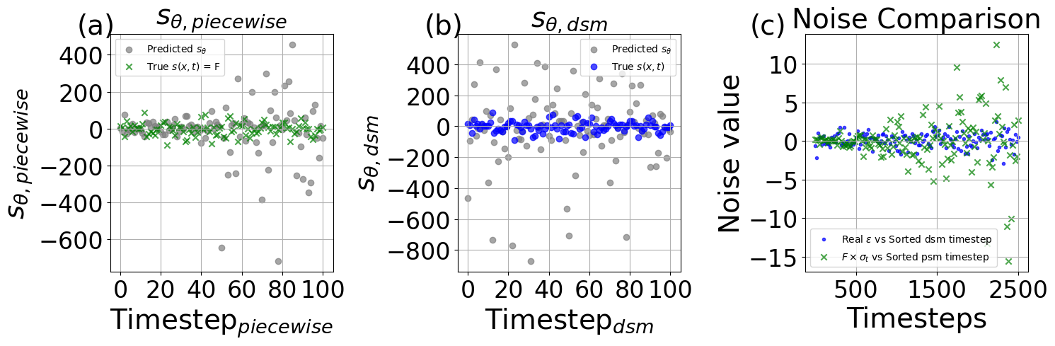
Figure 6: Comparison of the network $-\frac{\epsilon_{\theta}}{\sigma_{t}}$ and the noise. (a) Comparison of networks $-\frac{\epsilon_{\theta}}{\sigma_{t}}$ and labels $\bm{F}$ in $t\in[0,0.02]$; (b) Comparison of networks $-\frac{\epsilon_{\theta}}{\sigma_{t}}$ and random noise function $-\frac{\epsilon}{\sigma_{t}}$ in $t\in[0,0.02]$; (c)Two noise labels change with the noise addition time $t\in[0,0.5]$. The noise label for DSM is a random noise, and the noise label for PSM is $\bm{F}\sigma_{t}$.

(2) The Lipschitz problem of DSM.

Lemma 3.

Given the forward process $\bm{x}_{t}=\alpha_{t}\bm{x}_{0}+\sigma_{t}\bm{\epsilon}$, if the noise schedule satisfies $\sigma_{t}\to 0$ as $t\to 0$, then the Lipschitz constant of the neural network $\epsilon_{\theta}$ satisfies $\lim_{t\rightarrow 0}\sup\left\|\frac{\partial\epsilon_{\theta}(\bm{x}_{t},t)}{\partial t}\right\|_{2}\to\infty$.

Proof.

By $\epsilon_{\theta}=\sigma_{t}\cdot s_{\theta}\approx\sigma_{t}\cdot\nabla_{x}\log p\left(\bm{x}_{t}\right)$ and the chain rule, $\frac{\partial\epsilon_{\theta}}{\partial t}=-\frac{d\sigma_{t}}{dt}\nabla_{x}\log p\left(\bm{x}_{t}\right)-\frac{\partial\nabla_{x}\log p\left(\bm{x}_{t}\right)}{\partial t}\sigma_{t}.$ We assume that the $\nabla_{x}\log p\left(\bm{x}_{t}\right)$ is smooth. Since $\bm{x}_{t}=\alpha_{t}\bm{x}_{0}+\sigma_{t}\bm{\epsilon}$,

(i) VESDE: $\alpha_{t}=1,\,\sigma_{t}=\sigma_{0}\left(\frac{\sigma_{1}}{\sigma_{0}}\right)^{t}$, where $\sigma_{0}=\sigma_{\min}$, $\sigma_{1}=\sigma_{\max}$, then $\frac{d\sigma_{t}}{dt}=\sigma_{0}\left(\frac{\sigma_{1}}{\sigma_{0}}\right)^{t}\cdot\ln\frac{\sigma_{1}}{\sigma_{0}}=\sigma_{t}\cdot\ln\frac{\sigma_{1}}{\sigma_{0}}$. Therefore, $\frac{d\sigma_{t}}{dt}\nabla_{x}\log p\left(\bm{x}_{t}\right)$ has the order of $O(\ln\frac{\sigma_{1}}{\sigma_{0}}\cdot\bm{z})$, where $\bm{z}$ is the random noise. As [33] mentioned that, $\sigma_{0}$ approaches 0 theoretically, but in practice, $\sigma_{0}=0.01$ is taken to avoid singular values.

(ii) VPSDE: $\alpha_{t=}e^{-\frac{1}{2}\int_{0}^{t}\beta_{s}d_{s}},\,\sigma_{t}=\sqrt{1-e^{-\int_{0}^{t}\beta_{s}dt}}$, then $\frac{d\sigma_{t}}{dt}=-\beta_{t}\left(-e^{-\int_{0}^{t}\beta_{s}ds}\right)\left(1-e^{-\int_{0}^{t}\beta_{s}ds}\right)^{-\frac{1}{2}}=\frac{\beta_{t}e^{-\int_{0}^{t}\beta_{s}ds}}{\sqrt{1-e^{-\int_{0}^{t}\beta_{s}ds}}}\rightarrow+\infty\quad\text{ if }t\rightarrow 0^{+}$.

It shows the Lipschitz singularity property.

∎

Appendix C More Experimental Details

Dataset and settings.

The MD17 dataset and the MD22 dataset can be downloaded from http://quantum-machine.org/gdml/data/npz, the LJ13 and LJ55 data are from https://osf.io/srqg7/files/osfstorage. Hyperparameters for experiments are recorded in Table 6 and 7.

Table 6: Hyperparameters for different datasets with biased trainset

Dataset	Data Split	Batch Size	Max	Radius of
	(train, val, test)	(train, val)	Epochs	Graph
LJ13	First 1k, 0.1, remaining	(64, 64)	2000	4
LJ55	First 1k, 0.1, remaining	(64, 64)	2000	5
MD17	First 5k, 0.1, remaining	(64, 64)	1000	5
MD22 (Dw nanotube)	First 5k, 0.1, remaining	(8, 8)	3000	4
MD22 (others)	First 5k, 0.1, remaining	(16, 16)	500	7 (AT-AT)
				7 (AT-AT-CG-CG)
				6 (Ac-Ala3-NHMe)
				6 (Docosahexaenoic Acid)
				6 (Stachyose, Buckyballcatcher)
Additional Settings
Learning rate: $0.0002$  Lr scheduler: Cosine  Seed: $42$
Optimizer: Adam  Weight decay: $5\times 10^{-7}$
All diffusion parameters: $\sigma_{\text{min}}=0.1$, $\sigma_{\text{max}}=5$, time weight function $\lambda(t)=1$
Sampling timesteps: $1,000$  Sampling method: Predict-corrector sampler

Table 7: Hyperparameters compared with previous work in Table 2.

Dataset	Data Split	Batch Size	Max Epochs	Radius of Graph	Noise Schedule
	(train, val, test)	(train, val)
LJ13	0.1, 0.1, remaining	(64, 64)	5000	4	$\sigma_{\min}=0.01$, $\sigma_{\max}=8$
LJ55	0.1, 0.1, remaining	(64, 64)	5000	5	$\sigma_{\min}=0.01$, $\sigma_{\max}=4$
Additional Settings are the same as before in Table 6.

Lennard-Jones potential.

Here we additionally supplement the LJ potential with biased data training to obtain the energy comparisons in Figure 7.

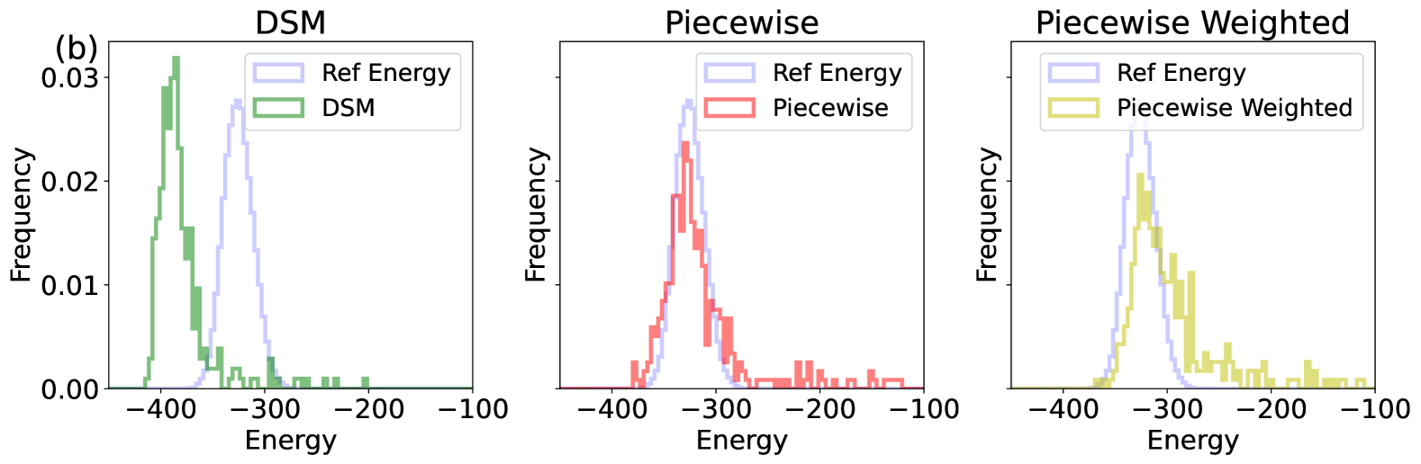
Figure 7: Comparisons of energy for (a) LJ-13 and (b) LJ-55 potential training with first $1,000$ data.

Appendix D Relationship with Flow Matching

Flow matching is a powerful tool for generating molecular conformations and predicting molecular properties [23, 5, 27]. It enables faster training and sampling while achieving superior generalization performance. Motivated by recent advancements [37, 10], unified frameworks have been developed to describe both diffusion models and flow matching methods comprehensively.

Let $\bm{y}_{0}$ and $\bm{y}_{1}$ be samples from the noise distribution and the data distribution, respectively, in the flow matching framework. As demonstrated in [10], the relationship between the velocity field and the score function is given by:

$$v(\bm{x},t)=\frac{\dot{\alpha}_{t}}{\alpha_{t}}\bm{x}+\gamma_{t}\left(\frac{\dot{\alpha}_{t}}{\alpha_{t}}\gamma_{t}-\dot{\gamma}_{t}\right)s(\bm{x},t),$$

where $\bm{x}_{t}=\alpha_{t}\bm{y}_{1}+\gamma_{t}\bm{y}_{0}=\alpha_{t}\bm{x}_{0}+\gamma_{t}\varepsilon$. Based on this relationship, our method can be extended to flow matching. In our setting, the coefficients are defined as follows:

$$\text{VE}:\,\,\alpha_{t}=1,\quad\gamma_{t}=\sigma_{t}=\sigma_{0}\left(\frac{\sigma_{1}}{\sigma_{0}}\right)^{t}\,,\quad\text{VP}:\,\,\alpha_{t}=e^{-\frac{1}{2}\int_{0}^{t}\beta_{s}ds},\quad\gamma_{t}=\left(1-e^{-\int_{0}^{t}\beta_{s}ds}\right)^{\frac{1}{2}}\,.$$ (30)

Therefore, the vector field $v(\bm{x},t)=\gamma_{t}\dot{\gamma}_{t}s(\bm{x},t)=\sigma_{0}^{2}\left(\frac{\sigma_{1}}{\sigma_{0}}\right)^{2t}\ln\left(\frac{\sigma_{1}}{\sigma_{0}}\right)s(\bm{x},t)$ for VESDE, and $v(\bm{x},t)=-\frac{1}{2}\beta_{t}\bm{x}+\gamma_{t}\left(-\frac{1}{2}\beta_{t}\gamma_{t}-\dot{\gamma}_{t}\right)s(\bm{x},t)$ for VPSDE. Building on the interplay between energy and the score function, we propose to investigate an energy-informed flow matching method. This energy-based extension will form the basis of our future research endeavors.

References

- [1] Tara Akhound-Sadegh, Jarrid Rector-Brooks, Avishek Joey Bose, Sarthak Mittal, Pablo Lemos, Cheng-Hao Liu, Marcin Sendera, Siamak Ravanbakhsh, Gauthier Gidel, Yoshua Bengio, et al. Iterated denoising energy matching for sampling from boltzmann densities. arXiv preprint arXiv:2402.06121, 2024.
- [2] Berni J Alder and Thomas Everett Wainwright. Studies in molecular dynamics. i. general method. The Journal of Chemical Physics, 31(2):459–466, 1959.
- [3] Fan Bao, Min Zhao, Zhongkai Hao, Peiyao Li, Chongxuan Li, and Jun Zhu. Equivariant energy-guided sde for inverse molecular design. In The eleventh international conference on learning representations, 2022.
- [4] Valentin De Bortoli, Michael Hutchinson, Peter Wirnsberger, and Arnaud Doucet. Target score matching, 2024.
- [5] Ricky TQ Chen and Yaron Lipman. Riemannian flow matching on general geometries. arXiv preprint arXiv:2302.03660, 2023.
- [6] Wenlin Chen, Mingtian Zhang, Brooks Paige, José Miguel Hernández-Lobato, and David Barber. Diffusive gibbs sampling. In Forty-first International Conference on Machine Learning, 2024.
- [7] Stefan Chmiela, Valentin Vassilev-Galindo, Oliver T. Unke, Adil Kabylda, Huziel E. Sauceda, Alexandre Tkatchenko, and Klaus-Robert Müller. Accurate global machine learning force fields for molecules with hundreds of atoms. Science Advances, 9(2):eadf0873.
- [8] Hyungjin Chung, Jeongsol Kim, Michael T Mccann, Marc L Klasky, and Jong Chul Ye. Diffusion posterior sampling for general noisy inverse problems. In The Eleventh International Conference on Learning Representations, ICLR 2023. The International Conference on Learning Representations, 2023.
- [9] Valentin De Bortoli, Emile Mathieu, Michael Hutchinson, James Thornton, Yee Whye Teh, and Arnaud Doucet. Riemannian score-based generative modelling. Advances in Neural Information Processing Systems, 35:2406–2422, 2022.
- [10] Carles Domingo-Enrich, Michal Drozdzal, Brian Karrer, and Ricky TQ Chen. Adjoint matching: Fine-tuning flow and diffusion generative models with memoryless stochastic optimal control. arXiv preprint arXiv:2409.08861, 2024.
- [11] Aleksander EP Durumeric, Yaoyi Chen, Frank Noé, and Cecilia Clementi. Learning data efficient coarse-grained molecular dynamics from forces and noise. arXiv preprint arXiv:2407.01286, 2024.
- [12] Lawrence C Evans. An introduction to stochastic differential equations, volume 82. American Mathematical Soc., 2012.
- [13] LawrenceCraig Evans. Measure theory and fine properties of functions. Routledge, 2018.
- [14] Xiang Fu, Zhenghao Wu, Wujie Wang, Tian Xie, Sinan Keten, Rafael Gomez-Bombarelli, and Tommi Jaakkola. Forces are not enough: Benchmark and critical evaluation for machine learning force fields with molecular simulations. arXiv preprint arXiv:2210.07237, 2022.
- [15] Andrew Gelman and Donald B Rubin. Markov chain monte carlo methods in biostatistics. Statistical methods in medical research, 5(4):339–355, 1996.
- [16] Jonathan Ho, Ajay Jain, and Pieter Abbeel. Denoising diffusion probabilistic models. Advances in neural information processing systems, 33:6840–6851, 2020.
- [17] Emiel Hoogeboom, Vıctor Garcia Satorras, Clément Vignac, and Max Welling. Equivariant diffusion for molecule generation in 3d. In International conference on machine learning, pages 8867–8887. PMLR, 2022.
- [18] Michael Janner, Yilun Du, Joshua Tenenbaum, and Sergey Levine. Planning with diffusion for flexible behavior synthesis. In International Conference on Machine Learning, pages 9902–9915. PMLR, 2022.
- [19] Tero Karras, Miika Aittala, Timo Aila, and Samuli Laine. Elucidating the design space of diffusion-based generative models. Advances in neural information processing systems, 35:26565–26577, 2022.
- [20] Jonas Köhler, Leon Klein, and Frank Noé. Equivariant flows: exact likelihood generative learning for symmetric densities. In International conference on machine learning, pages 5361–5370. PMLR, 2020.
- [21] Tuan Le, Frank No’e, and Djork-Arné Clevert. Equivariant graph attention networks for molecular property prediction. ArXiv, abs/2202.09891, 2022.
- [22] Yi-Lun Liao, Brandon Wood, Abhishek Das*, and Tess Smidt*. EquiformerV2: Improved Equivariant Transformer for Scaling to Higher-Degree Representations. In International Conference on Learning Representations (ICLR), 2024.
- [23] Yaron Lipman, Ricky TQ Chen, Heli Ben-Hamu, Maximilian Nickel, and Matt Le. Flow matching for generative modeling. arXiv preprint arXiv:2210.02747, 2022.
- [24] Calvin Luo. Understanding diffusion models: A unified perspective. arXiv preprint arXiv:2208.11970, 2022.
- [25] J Andrew McCammon, Bruce R Gelin, and Martin Karplus. Dynamics of folded proteins. nature, 267(5612):585–590, 1977.
- [26] Laurence Illing Midgley, Vincent Stimper, Gregor NC Simm, Bernhard Schölkopf, and José Miguel Hernández-Lobato. Flow annealed importance sampling bootstrap. arXiv preprint arXiv:2208.01893, 2022.
- [27] Benjamin Kurt Miller, Ricky TQ Chen, Anuroop Sriram, and Brandon M Wood. Flowmm: Generating materials with riemannian flow matching. arXiv preprint arXiv:2406.04713, 2024.
- [28] Albert Musaelian, Simon Batzner, Anders Johansson, Lixin Sun, Cameron J Owen, Mordechai Kornbluth, and Boris Kozinsky. Learning local equivariant representations for large-scale atomistic dynamics. Nature Communications, 14(1):579, 2023.
- [29] Frank Noé, Simon Olsson, Jonas Köhler, and Hao Wu. Boltzmann generators: Sampling equilibrium states of many-body systems with deep learning. Science, 365(6457):eaaw1147, 2019.
- [30] Angus Phillips, Hai-Dang Dau, Michael John Hutchinson, Valentin De Bortoli, George Deligiannidis, and Arnaud Doucet. Particle denoising diffusion sampler. In Forty-first International Conference on Machine Learning, 2024.
- [31] Chence Shi, Shitong Luo, Minkai Xu, and Jian Tang. Learning gradient fields for molecular conformation generation. In International conference on machine learning, pages 9558–9568. PMLR, 2021.
- [32] Jiaming Song, Chenlin Meng, and Stefano Ermon. Denoising diffusion implicit models. In International Conference on Learning Representations, 2020.
- [33] Yang Song, Jascha Sohl-Dickstein, Diederik P Kingma, Abhishek Kumar, Stefano Ermon, and Ben Poole. Score-based generative modeling through stochastic differential equations. In International Conference on Learning Representations, 2020.
- [34] Gabriel Stoltz, Mathias Rousset, et al. Free energy computations: A mathematical perspective. World Scientific, 2010.
- [35] Francisco Vargas, Will Sussman Grathwohl, and Arnaud Doucet. Denoising diffusion samplers. In International Conference on Learning Representations, 2023.
- [36] Yan Wang, Lihao Wang, Yuning Shen, Yiqun Wang, Huizhuo Yuan, Yue Wu, and Quanquan Gu. Protein conformation generation via force-guided se (3) diffusion models. arXiv preprint arXiv:2403.14088, 2024.
- [37] Dongyeop Woo and Sungsoo Ahn. Iterated energy-based flow matching for sampling from boltzmann densities. arXiv preprint arXiv:2408.16249, 2024.
- [38] Fang Wu and Stan Z Li. Diffmd: a geometric diffusion model for molecular dynamics simulations. In Proceedings of the AAAI Conference on Artificial Intelligence, volume 37, pages 5321–5329, 2023.
- [39] Kevin E Wu, Kevin K Yang, Rianne van den Berg, Sarah Alamdari, James Y Zou, Alex X Lu, and Ava P Amini. Protein structure generation via folding diffusion. Nature Communications, 15(1):1059, 2024.
- [40] Minkai Xu, Lantao Yu, Yang Song, Chence Shi, Stefano Ermon, and Jian Tang. Geodiff: A geometric diffusion model for molecular conformation generation. In International Conference on Learning Representations, 2022.
- [41] Zhantao Yang, Ruili Feng, Han Zhang, Yujun Shen, Kai Zhu, Lianghua Huang, Yifei Zhang, Yu Liu, Deli Zhao, Jingren Zhou, et al. Lipschitz singularities in diffusion models. In The Twelfth International Conference on Learning Representations, 2023.
- [42] Qinsheng Zhang and Yongxin Chen. Path integral sampler: a stochastic control approach for sampling. In International Conference on Learning Representations, 2022.