Online Conformal Probabilistic Numerics via
Adaptive Edge-Cloud Offloading

Abstract

Consider an edge computing setting in which a user submits queries for the solution of a linear system to an edge processor, which is subject to time-varying computing availability. The edge processor applies a probabilistic linear solver (PLS) so as to be able to respond to the user’s query within the allotted time and computing budget. Feedback to the user is in the form of an uncertainty set. Due to model misspecification, the uncertainty set obtained via a direct application of PLS does not come with coverage guarantees with respect to the true solution of the linear system. This work introduces a new method to calibrate the uncertainty sets produced by PLS with the aim of guaranteeing long-term coverage requirements. The proposed method, referred to as online conformal prediction-PLS (OCP-PLS), assumes sporadic feedback from cloud to edge. This enables the online calibration of uncertainty thresholds via online conformal prediction (OCP), an online optimization method previously studied in the context of prediction models. The validity of OCP-PLS is verified via experiments that bring insights into trade-offs between coverage, prediction set size, and cloud usage.

1 Introduction

In modern hierarchical computing architectures encompassing edge and cloud segments, the efficient management of computational resources is critical to balance performance with latency and communication overhead. For instance, in industrial Internet-of-Things (IoT) settings, sensor data processing must integrate real-time decision-making at the edge with more complex analytics in the cloud, while accounting for inherent trade-offs between response speed and accuracy (Hong et al., 2019).

Linear systems serve as the cornerstone of virtually all numerical computation. These systems – in the form of the equation $Ax=b$ with unknown vector $x$ – arise in contexts including convex optimization (Boyd and Vandenberghe, 2004), Kalman filtering for state estimation (Thrun, 2002), and finite element analysis for computational fluid dynamics (Gassner and Winters, 2021). A timely and efficient solution of such systems is often critical for real-time decision-making.

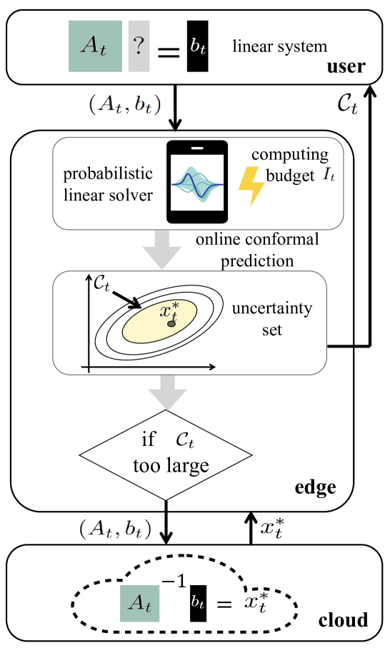
Figure 1: At each round $t$, a user submits a linear system defined by the pair $(A_{t},b_{t})$ to an edge device. Given the available computing budget $I_{t}$, the edge device employs a probabilistic linear solver (PLS), obtaining an uncertainty set $\mathcal{C}_{t}$ for the true solution $x^{*}_{t}=A_{t}^{-1}b_{t}$. The set $\mathcal{C}_{t}$ is returned in a timely fashion to the user. The proposed method, OCP-PLS ensures long-term coverage guarantees (2) for the uncertainty sets $\mathcal{C}_{t}$, addressing model misspecification in PLS. To this end, OCP-PLS allows for sporadic communication between cloud and edge.

As illustrated in Fig. 1, we consider an edge computing scenario in which, at each round $t=1,2,...$, a user submits a query for the solution of a linear system $A_{t}x_{t}=b_{t}$ to an edge processor, which is subject to time-varying computing power availability. The user seeks to obtain timely information about the solution $x_{t}^{*}=A_{t}^{-1}b_{t}$. However, a direct evaluation of the solution requires cubic computational complexity with respect to the matrix dimension, which may be infeasible within the given latency and computing budgets (Wenger and Hennig, 2020; Cockayne et al., 2019a).

Iterative solvers provide an ideal solution to adapt to the available computing budget, as they refine the solution sequentially until the computing budget runs out. Specifically, probabilistic numerics (PN) (Larkin, 1972) treats numerical problems, such as solving linear systems, as a form of statistical inference. This provides a natural way to quantify the uncertainty associated with iterative numerical solutions obtained under limited computing power.

Specifically, probabilistic linear solvers (PLSs) (Cockayne et al., 2019a; Hennig et al., 2015; Bartels et al., 2019; Reid et al., 2020; Pförtner et al., 2024) treat the solution of a linear system as a Bayesian inference problem, whereby each iteration provides an updated posterior distribution for the solution $x^{*}_{t}$. The posterior distribution reflects the current knowledge of the true solution given the available computing budget. Using this posterior distribution, PLS can construct an uncertainty set $\mathcal{C}_{t}$ with the aim of covering the true solution $x^{*}_{t}$ with a pre-determined target probability level.

In the considered system illustrated in Fig. 1, at each round $t$, the edge processor applies PLS so as to be able to respond to the user’s query within the allotted time and computing budgets. Feedback to the user is in the form of an uncertainty set $\mathcal{C}_{t}$. However, in the presence of model misspecification, the uncertainty sets obtained using a direct application of PLS do not come with coverage guarantees with respect to the true solution $x^{*}_{t}$ of the linear system (Cockayne et al., 2019a; Bartels et al., 2019; Wenger and Hennig, 2020; Hennig et al., 2015), and are often too conservative (Hegde et al., 2024; Reid et al., 2020; Wenger and Hennig, 2020). Note that misspecification in PLS often occurs during its iterative update procedure, which comes as a cost to accelerate the computing speed (Cockayne et al., 2019a, 2022, b).

This work introduces a new method to calibrate the uncertainty sets produced by PLS with the aim of guaranteeing long-term coverage requirements, while addressing the excessive conservativeness of PLS. In practice, we wish to ensure that, on average over time, the uncertainty set $\mathcal{C}_{t}$ returned by the edge to the user contains the true solution $x^{*}_{t}$ with a user-defined coverage rate $1-\alpha$.

To ensure this condition, we assume that, sporadically, the edge processor can submit the current linear system defined by the pair $(A_{t},b_{t})$ to a cloud processor. This offloading to the cloud is done after responding to a user’s query in order not to affect the latency experienced by the user. When submitting the job to the cloud, the edge processor receives the true solution $x^{*}_{t}$. This information can be used to monitor the current coverage rate, making it possible to calibrate the prediction sets $\mathcal{C}_{t}$ towards meeting the required target rate $1-\alpha$.

The proposed method, referred to as online conformal prediction-PLS (OCP-PLS), integrates for the first time PLS with online conformal prediction (OCP), an online optimization method previously studied in the context of predictive models (Gibbs and Candes, 2021; Angelopoulos et al., 2024). The theoretical validity of OCP-PLS is verified via experiments that bring insights into trade-offs between coverage, prediction set size, and cloud usage.

The structure of the paper is as follows. Section 2 introduces the problem of conformal PLS. The necessary background on OCP is reviewed in Section 3. Section 4 presents the proposed approaches for constructing OCP-PLS. Simulation results are summarized in Section 5. Finally, Section 6 concludes the paper.

2 Setting and Problem Formulation

In this section, we define the problem studied in this paper.

2.1 Setting and Problem Definition

As illustrated in Fig. 1, we study a hierarchical computing architecture encompassing edge and cloud processors. At each round $t$, a user submits a linear system problem defined by the pair $(A_{t},b_{t})$, consisting of an $n_{t}\times n_{t}$ Hermitian matrix $A_{t}$ and an $n_{t}\times 1$ vector $b_{t}$, to the edge device. The user is interested in obtaining information about the optimal solution

$$x^{*}_{t}=A_{t}^{-1}b_{t}.$$ (1)

This solution is supposed to exist and to be unique, requiring matrix $A_{t}$ to be invertible. Problems of this type are common in a wide variety of applications, such as convex optimization using Newton’s method requiring Hessian matrix inversion (Boyd and Vandenberghe, 2004), Kalman filtering for state estimation (Thrun, 2002), and partial differential equations in computational fluid dynamics via Galerkin’s method (Gassner and Winters, 2021).

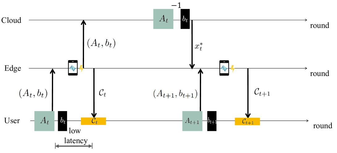
Figure 2: Timeline of messages exchanged across cloud, edge, and user.

At each round $t$, the edge has available a computing budget $I_{t}$. Accounting for this limited budget, the edge device employs PLS to obtain an uncertainty set $\mathcal{C}_{t}$ for the true solution (1) (Cockayne et al., 2019a; Bartels et al., 2019; Wenger and Hennig, 2020). This set is returned to the user in response to its query. Thanks to processing at the edge, the uses’ requests experience low latency (see Fig. 2).

This paper addresses the problem of calibrating the prediction set $C_{t}$ so as to ensure that the sequence of uncertainty sets $C_{t}$ returned to the user satisfies the following long-term coverage condition

$$\left|\frac{1}{T}\sum_{t=1}^{T}\Pr\{x_{t}^{*}\in\mathcal{C}_{t}\}-(1-\alpha)\right|\leq o(1),$$ (2)

where $\alpha\in[0,1]$ is a pre-determined target miscoverage level, and $o(1)$ denotes a quantity that tends to zero as $T\rightarrow\infty$. The probability (2) is evaluated over the randomness associated with edge-cloud communication, as it will be described in Section 4. By (2), a fraction approximately equal to $1-\alpha$ of the prediction sets contains the true solution $x^{*}_{t}$.

As shown in Fig. 2, after responding to the user, the edge processor analyzes the prediction set $\mathcal{C}_{t}$, and decides whether to submit the problem $(A_{t},b_{t})$ for validation to the cloud. If the edge processor communicates the pair $(A_{t},b_{t})$ to the cloud, the cloud evaluates the true solution $x^{*}_{t}$ and returns it to the edge. This allows the edge to monitor the condition (2), and to calibrate future sets $C_{t^{\prime}}$ with $t^{\prime}>t$. However, cloud-based validation is expensive, and the edge aims at keeping the number of problems submitted to the cloud as low as possible. As shown in Fig. 2, we will assume first that feedback from the cloud, if requested, is received prior to the next query $(A_{t+1},b_{t+1})$ by the user. This assumption will be alleviated in the appendix.

2.2 Probabilistic Linear Solver

As previously mentioned, the edge processor addresses the problem $(A_{t},b_{t})$ within the computing budget $I_{t}$ using PLS. Accordingly, PLS treats the solution of a linear system as a Bayesian inference problem. This enables the quantification of the uncertainty associated with numerical solutions obtained within a limited computing budget (Cockayne et al., 2019a; Bartels et al., 2019; Wenger and Hennig, 2020).

Given a budget of $I_{t}$ iteration, PLS operates sequentially by considering at each iteration $i=1,\ldots,I_{t}$ a search direction $s_{i}$, yielding an effective observation $y_{i}=s_{i}^{T}b$. Given a Gaussian prior distribution $x^{*}\sim\mathcal{N}(\mu_{0},\Sigma_{0})$ on the solution $x^{*}=A_{t}^{-1}b_{t}$, PLS returns the Gaussian posterior

$$p(x_{t}|y_{1},\dots,y_{I_{t}};A_{t},b_{t})=\mathcal{N}(x_{t}|\mu_{t},\Sigma_{t})$$ (3)

obtained from the observations $y_{1},\dots,y_{I_{t}}$. In (3), the $d\times 1$ mean vector $\mu_{t}$ and the $d\times d$ covariance matrix $\Sigma_{t}$ are evaluated as (Cockayne et al., 2019a; Bartels et al., 2019)

$$\mu_{t} =\mu_{0}+\Sigma_{0}A_{t}S_{t}(S_{t}^{\top}A_{t}\Sigma_{0}A_{t}S_{t})^{-1}S_{t}^{\top}(b-A_{t}\mu_{0}),$$ (4)

$$\Sigma_{t} =\Sigma_{0}-\Sigma_{0}A_{t}S_{t}(S_{t}^{\top}A_{t}\Sigma_{0}A_{t}S_{t})^{-1}S_{t}^{\top}A_{t}\Sigma_{0},$$

with the $d\times I_{t}$ matrix

$$S_{t}=[s_{1},...,s_{I_{t}}]$$ (5)

collecting the $I_{t}$ search directions.

Given the posterior distribution (3), an $(1-\alpha)$-uncertainty set for the true solution $x^{*}_{t}$ can be obtained as

$$\mathcal{C}_{t}= \mathop{\rm{argmin}}\limits_{\mathcal{C}\subseteq\mathbb{R}^{d}}\ |\mathcal{C}|$$

$$\text{ s.t. }\int_{x_{t}\in\mathcal{C}}p(x_{t}|A_{t},b_{t})\mathrm{d}x_{t}\geq 1-\alpha,$$ (6)

where we wrote $p(x_{t}|A_{t},b_{t})$ in lieu of $p(x_{t}|y_{1},\dots,y_{I_{t}};A_{t},b_{t})$ to simplify the notation.

The uncertainty set (2.2) covers the true solution $x^{*}_{t}$ in (1) with probability no smaller than $1-\alpha$, i.e.,

$$\Pr[x^{*}_{t}\in\mathcal{C}_{t}]\geq 1-\alpha,$$ (7)

only if the posterior distribution $p(x_{t}|A_{t},b_{t})$ is able to describe the true uncertainty on the solution $x^{*}_{t}$ given the observation $y_{1},\dots,y_{I_{t}}$, i.e., $p(x_{t}|A_{t},b_{t})$ is well calibrated.

However, the PLS posterior (3) is known to be generally poorly calibrated because of model misspecification (Cockayne et al., 2019a; Bartels et al., 2019; Wenger and Hennig, 2020; Hennig et al., 2015). Therefore, there is a need to develop model selection to satisfy the coverage requirement (2). This is the main objective of this work.

3 Background

This section reviews the necessary background on OCP (Gibbs and Candes, 2021; Zhao et al., 2024).

3.1 Online Conformal Prediction

Given an arbitrary sequence of input-output pairs $(x_{t},y_{t})\in\mathcal{X}\times\mathcal{Y}$, for $t=1,2,\ldots$, OCP aims to construct a prediction set $\mathcal{C}_{t}(x_{t})$ on the output space $\mathcal{Y}$ that satisfies long-term coverage guarantees. OCP builds on a scoring function $s:\mathcal{X}\times\mathcal{Y}\rightarrow\mathbb{R}$ that measures the extent to which the output $y$ is mismatched to the input $x$. A smaller value $s(x,y)$ indicates that $y$ is a better fit for input $x$. The set $\mathcal{C}_{t}(x_{t})$ is obtained by choosing all the candidate output values $y\in\mathcal{Y}$ with sufficiently small scores $s(x,y)$, i.e.,

$$\mathcal{C}_{t}(x_{t})=\{y\in\mathcal{Y}:s(x_{t},y)\leq\lambda_{t}\},$$ (8)

where $\lambda_{t}$ is a threshold.

OCP updates the threshold $\lambda_{t}$ in (8) based on the input-output pairs $(x_{1},y_{1}),\ldots,(x_{t-1},y_{t-1})$ with the aim of ensuring the long-term coverage condition

$$\left|\frac{1}{T}\sum_{t=1}^{T}\mathds{1}\{y_{t}\in\mathcal{C}_{t}(x_{t})\}-(1-\alpha)\right|\leq\frac{C}{T},$$ (9)

where $C$ is a constant independent of $T$. This result is obtained by updating the threshold as

$$\lambda_{t+1}=\lambda_{t}+\gamma\big{(}\mathds{1}\{y_{t}\not\in\mathcal{C}_{t}(x_{t})\}-\alpha\big{)},$$ (10)

where $\gamma>0$ is a step size. This update rule intuitively increases the threshold when the prediction set $\mathcal{C}_{t}(x_{t})$ fails to cover the true outcome $y_{t}$, making future sets more conservative, while decreasing it when coverage is achieved, making future sets more efficient.

The validity of the condition (9) for the prediction sets (8) obtained via the OCP update rule (10) were shown in Gibbs and Candes (2021) using a telescoping argument, obtaining

$$C=\max\frac{|\lambda_{T+1}-\lambda_{1}|}{\gamma}.$$ (11)

If the score function $s(x,y)$ is bounded within the interval $[m,M]$ with $M>m$ for any $(x,y)\in\mathcal{X}\times\mathcal{Y}$, then the threshold $\lambda_{t}$ can be also proved to be bounded as $\lambda_{t}\in[m-\gamma\alpha,M+\gamma(1-\alpha)]$, where $\lambda_{1}$ is selected within the interval $[m,M]$ (Gibbs and Candes, 2021). Accordingly, the quantity (11) is given as

$$C=\frac{M-m+\gamma}{\gamma},$$ (12)

which does not depend on $T$.

3.2 Intermittent Online Conformal Prediction

The OCP update (10) requires dense feedback, as it assumes the availability of the true output $y_{t}$ at every time step $t=1,2,...$ in (10). Intermittent OCP (I-OCP) (Zhao et al., 2024) alleviates this assumption by leveraging inverse probability weighting, also known as the Horvitz-Thompson estimator, which is used in statistical inference with missing data (Imbens and Rubin, 2015).

Specifically, I-OCP assumes that the output $y_{t}$ is available with probability $p_{t}$. The availability of the output is thus described by a Bernoulli random variable $\text{obs}_{t}\sim\text{Bern}(p_{t})$, which indicates the availability of the output value $y_{t}$ if $\text{obs}_{t}=1$, and its absence when $\text{obs}_{t}=0$. The variables $\text{obs}_{t}$ are independent over the time index $t$. The update rule applied by I-OCP is given by

$$\lambda_{t+1}=\lambda_{t}+\frac{\gamma}{p_{t}}\big{(}\mathds{1}\{y_{t}\not\in\mathcal{C}_{t}(x_{t})\}-\alpha\big{)}\cdot\text{obs}_{t}.$$ (13)

Thus, I-OCP amplifies the update of the threshold to an extent that is inversely proportional to the availability probability $p_{t}$. Accordingly, when feedback is less likely, i.e., when $p_{t}$ is smaller, the effective step size is increased to compensate for possible missing data.

It can be proved that I-OCP satisfies the long-term expected coverage property

$$\left|\frac{1}{T}\sum_{t=1}^{T}\Pr\big{[}y_{t}\in\mathcal{C}_{t}(x_{t})\big{]}-(1-\alpha)\right|\leq\frac{C}{T}$$ (14)

with $C$ in (11), where the probability is evaluated over the randomness of the Bernoulli random variables
$\text{obs}_{1},\ldots,\text{obs}_{T}$.

In a manner similar to OCP, as long as the score function $s(x,y)$ is bounded in the interval $[m,M]$ for any $(x,y)\in\mathcal{X}\times\mathcal{Y}$, it can be shown that the quantity $C$ in (14) is also bounded. Specifically, denote as $p^{\text{min}}_{t}$ the lowest value that can be attained by the probability $p_{t}$. Note that the probability $p_{t}$ can generally depend on the previous history $(x_{1},y_{1}),\ldots,(x_{t-1},y_{t-1})$. Then, the threshold $\lambda_{t}$ is bounded as

$$\small\lambda_{t}\in\bigg{[}m-\gamma\frac{\alpha}{\min_{t^{\prime}=1,...,t-1}{{p}^{\text{min}}_{t^{\prime}}}},M+\gamma\frac{1-\alpha}{\min_{t^{\prime}=1,...,t-1}{{p}^{\text{min}}_{t^{\prime}}}}\bigg{]}$$ (15)

as long as one sets $\lambda_{1}\in[m,M]$. Accordingly, we have

$$C=\frac{M-m}{\gamma}+\frac{1}{\bar{p}_{T}},$$ (16)

for any

$$\bar{p}_{T}=\min_{t^{\prime}=1,...,T}{p}^{\text{min}}_{t}.$$ (17)

This quantity does not depend on $T$ if a strictly positive $\bar{p}$ exists with

$$\bar{p}_{T}\geq\bar{p}$$ (18)

for all times $T$.

4 Online Conformal Probabilistic Linear Solver

In this section, we present OCP-PLS, a novel framework for edge inference via PN that satisfies the quality-of-service requirement (2) by integrating PLS (see in Section 2.2) with I-OCP (see Section 3).

4.1 Score Function

As discussed in Section 3.1, OCP requires the definition of a score function for any value of the target variable. In the setting described in Section 2, the target variable at each time $t$ is the true solution $x^{*}_{t}$ in (1). Given the posterior distribution (3)-(4) produced by PLS, we set the score for any candidate solution $x_{t}$ to be proportional to the density $\mathcal{N}(x_{t}|\mu_{t},\Sigma_{t})$ as

$$s(x_{t};A_{t},b_{t})=\text{exp}\left(-(x_{t}-\mu_{t})^{T}\Sigma_{t}^{-1}(x-\mu_{t})\right).$$ (19)

Note that the score (19) depends on the specific sequence of search directions (5), although we do not make this dependence explicit in the notation $s(x_{t};A_{t},b_{t})$.

Equipped with the scoring function (19), OCP-PLS produces a prediction set of the form

$$\mathcal{C}_{t}=\{x_{t}\in\mathbb{R}^{d}:s(x_{t}:A_{t},b_{t})\geq\lambda_{t}\},$$ (20)

with a suitably designed threshold $\lambda_{t}$.

Two observations are in order about the OCP-PLS set (20). First, the PLS set (2.2) can be seen to take the same form as (20). However, PLS selects the threshold $\lambda_{t}$ by imposing the constraint in (2.2), which satisfies the requirement (2) only if the model is well specified. In contrast, as discussed in Section 4.2, OCP-PLS sets the threshold $\lambda_{t}$ by following the principles of OCP (see Section 3).

Second, computing the inverse $\Sigma_{t}^{-1}$ in (19) generally requires a complexity of the order $O(n_{t}^{3})$, which would not be feasible under the edge budget constraint. However, given the structure of the covariance matrix $\Sigma_{t}$ in (4) and assuming the use of conjugate gradient search directions (Cockayne et al., 2019a; Bartels et al., 2019), the inverse $\Sigma_{t}^{-1}$ can be computed efficiently using the Sherman-Morrison-Woodbury formula (Miller, 1981) at a complexity of the order $\mathcal{O}(I_{t}n_{t}^{2})$ (Hegde et al., 2024).

4.2 Cloud-to-Edge Feedback and Threshold Selection

As illustrated in Fig. 1 and Fig. 2, in order to set the threshold $\lambda_{t}$ in (20), OCP-PLS leverages sporadic feedback from the cloud to the edge. Specifically, we propose to submit a query $(A_{t},b_{t})$ to the cloud with a probability $p_{t}$ that increases with the size of the uncertainty set $\mathcal{C}_{t}$, i.e.,

$$|\mathcal{C}_{t}|=\frac{\pi^{n_{t}/2}}{\Gamma(n_{t}/2+1)}\cdot(\text{det}(\Sigma_{t}))^{1/2}\cdot(-\log\lambda_{t})^{n_{t}/2},$$ (21)

where $\Gamma(\cdot)$ is the Gamma function and $\text{det}(\cdot)$ is the determinant operator. In this way, cloud-to-edge feedback is more likely to be requested at time instants $t$ characterized by a larger uncertainty, hence making cloud feedback more valuable for calibration. Conversely, when the uncertainty set is small enough, we reduce the probability of requesting feedback, thereby saving cloud computing resources.

While any normalized increasing function of the set size $|\mathcal{C}_{t}|$ can be used to design $p_{t}$, we adopt the sigmoid function $\sigma(x)=\left(1+\text{exp}(-x)\right)^{-1}$ and set as

$$p_{t}=\sigma\left(\frac{\log|\mathcal{C}_{t}|}{n_{t}}-\theta\right),$$ (22)

which is a function of the log value of the set size normalized by the matrix dimension $n_{t}$. Lower values of hyperparameter $\theta$ in (22) increase the probability of cloud-to-edge feedback, yielding a smaller set $\mathcal{C}_{t}$ at the cost of higher usage of cloud resources.

Leveraging the feedback from the cloud, OCP-PLS targets the requirement (2) by updating the threshold according to the rule

$$\lambda_{t+1}=\lambda_{t}-\frac{\gamma}{p_{t}}(\text{err}_{t}-\alpha)\cdot\text{obs}_{t},$$ (23)

where the error at round $t$ is defined as

$$\text{err}_{t}=\mathds{1}\{x^{*}_{t}\notin\mathcal{C}_{t}\}.$$ (24)

The rule (23) is aligned with the I-OCP update (13). As formalized next, this ensures the validity of the coverage condition (2). The overall OCP-PLS procedure is summarized in Algorithm 1.

1:set hyperparameters $\lambda_{1}\in[0,1]$, $\gamma$, $\theta$ $\triangleright$ initialization

2:for $t=1,2,\dots,T$ do

3:  apply PLS with $I_{t}$ iterations to evaluate $\mu_{t}$ and $\Sigma_{t}$ in (4)

4:  evaluate the probability $p_{t}$ in (22)

5:  draw $\text{obs}_{t}\sim\text{Bern}(p_{t})$

6:  evaluate the uncertainty set $\mathcal{C}_{t}$ in (20)

7:  if $\text{obs}_{t}=1$ then

8:   obtain $x^{*}_{t}$ from the cloud

9:   $\text{err}_{t}=\mathds{1}\{s(x^{*}_{t};A_{t},b_{t})<\lambda_{t}\}$

10:  else

11:   $\lambda_{t+1}=\lambda_{t}$

12:  end if

13:end for

Algorithm 1 OCP-PLS

4.3 Theoretical Coverage Guarantee

OCP-PLS ensures condition (2) in the following way.

Proposition 1.

Assume that there exists a strictly positive probability $\bar{p}$ satisfying the inequality (18) for all times $T$. Then, OCP-PLS satisfies the long-term coverage property

$$\left|\frac{1}{T}\sum_{t=1}^{T}\Pr\big{[}x^{*}_{t}\in\mathcal{C}_{t}\big{]}-(1-\alpha)\right|\leq\frac{C}{T},$$ (25)

with constant

$$C=\frac{1}{\gamma}+\frac{1}{\bar{p}}.$$ (26)

Proof.

This result follows directly from Section 3.2 by noting that $s(x_{t};A_{t},b_{t})$ in (19) is bounded in $[0,1]$. ∎

5 Experiments

This section evaluates the performance of the proposed OCP-PLS scheme via numerical experiments.

5.1 Setup

At each round $t$, we randomly and independently generate a Hermitian matrix $A_{t}$ as $A_{t}=Q_{t}\Lambda_{t}Q_{t}$, where $n_{t}\times n_{t}$ orthogonal matrix $Q_{t}$ follows the Haar distribution and the diagonal matrix $\Lambda_{t}$ has diagonal elements drawn from a Gamma distribution with shape parameter $10$, scale parameter $1$, and location parameter $0$. The dimension $n_{t}$ is drawn i.i.d. and uniformly from the interval $[500,1000]$. Furthermore, each element of vector $b_{t}$ is sampled i.i.d. from the standard multivariate Gaussian distribution. We set the target miscoverage rate $\alpha$ as $0.1$. The step size $\gamma$ and initial threshold $\lambda_{1}$ are set as $0.05$ and $0.95$, respectively. For the hyperparameter $\theta$, we use grid search to find a suitable one as $-5.5$.

We consider two different scenarios in terms of edge processing power availability:

• Constant edge computing budget: In this case, the computing budget is set as a fixed fraction of the problem size as $I_{t}=0.1n_{t}$.

• Time-varying edge computing budget: In this more challenging scenario, the number of allowed iterations starts at $I_{t}=0.1n_{t}$ for $t=1$ to $t=1500$, then it decreases to $I_{t}=0.05n_{t}$ for $t=1500$ to $t=3500$, and finally it increases to $I_{t}=0.15n_{t}$ for $t=3500$ to $t=5000$.

5.2 Baselines

We consider the following baselines:

• PLS: Conventional PLS directly adopts the $(1-\alpha)$ uncertainty set as in (2.2).

• OCP-PLS with full cloud-to-edge feedback: This corresponds to the proposed OCP-PLS method with probability $p_{t}=1$ of acquiring feedback from cloud to edge.

5.3 Performance Metrics

As performance measures, we report empirical coverage, empirical uncertainty set size, and empirical cloud-to-edge feedback rate evaluated on a sequence $\{A_{t},b_{t}\}_{t=1}^{T}$ of duration $T=5000$. The empirical coverage at round $t$ measures the fraction of times in which the exact solution $x^{*}_{\tau}$ was included in the corresponding uncertainty set $\mathcal{C}_{t}$ from time $\tau=1$ until time $\tau=t$, i.e.,

$$\text{empirical coverage}=\frac{1}{t}\sum_{\tau=1}^{t}\mathds{1}\{x^{*}_{\tau}\in\mathcal{C}_{\tau}\}.$$ (27)

The empirical uncertainty set size at time step $t$ is defined as

$$\text{empirical set size}=\frac{1}{t}\sum_{\tau=1}^{t}|\mathcal{C}_{\tau}|.$$ (28)

Finally, the empirical cumulative cloud-to-edge feedback rate is defined as

empirical cumulative $$\text{ cloud-to-edge feedback rate}=\sum_{\tau=1}^{t}\text{obs}_{\tau}.$$ (29)

We average the probability (27)-(29) over $10$ independent experiments.

5.4 Results

In this subsection, we evaluate coverage, average set size, and cumulative cloud-to-edge feedback rate starting from the case with a constant edge computing budget.

Fig. 3(a) demonstrates that both OCP-PLS and OCP-PLS with full cloud-to-edge feedback guarantee the long-term coverage condition (2), thereby validating Proposition 1. In contrast, confirming prior art (Hegde et al., 2024; Wenger and Hennig, 2020), PLS produces an overly conservative uncertainty set that always covers the true solution. PLS achieves coverage of $1$ by yielding much larger uncertainty sets than both OCP-PLS and OCP-PLS with full cloud-to-edge feedback, as shown in Fig. 3(b). Furthermore, as illustrated in (2), OCP-PLS can reduce the cloud-to-edge feedback rate by approximately $40\%$ as compared to OCP-PLS with full cloud-to-edge feedback, while producing sets with similar sizes.

Consider now the setting with a time-varying computing budget at the edge. Fig. 4 marks the times at which the computing budget changes with vertical dashed lines. Fig. 4(a) verifies that both OCP-PLS and OCP-PLS with full cloud-to-edge feedback maintain the guaranteed long-term coverage condition proved in Proposition 1 even under time-varying computing budgets. As in the previous example, PLS provides perfect coverage at the cost of excessively large uncertainty sets. In contrast, as shown in Fig. 4(b), OCP-PLS responds naturally to changes in edge computing budget, as the set sizes increase during periods of reduced computing budget ($t=1500$ to $t=3500$), while decreasing when the computing budget is higher ($t=3500$ to $t=5000$). Throughout these variations, OCP-PLS consistently maintains a significantly lower cloud-to-edge feedback rate than OCP-PLS with full cloud-to-edge feedback, as shown in Fig. 4(c), adapting the feedback rate to the varying computing budgets. This demonstrates OCP-PLS’s ability to balance reliability and communication efficiency under dynamic edge computing budgets.

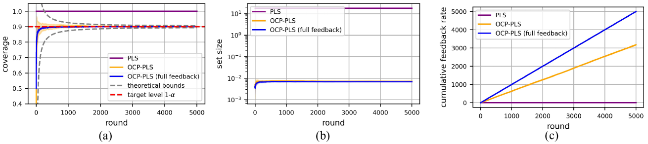
Figure 3: Coverage (a), set size (b), and cumulative cloud-to-edge feedback rate (c) for PLS, OCP-PLS, and OCP-PLS with full cloud-to-edge feedback for target coverage level $1-\alpha=0.9$ (red dashed line in (a)). The gray dashed line in (a) corresponds to the threshold bound (14).

Figure 4: Coverage (a), set size (b), and cumulative cloud-to-edge feedback rate (c) for PLS, OCP-PLS, and OCP-PLS with full cloud-to-edge feedback for target coverage level $1-\alpha=0.9$ (red dashed line in (a)) in a setting with time-varying edge computing budget. The gray dashed line in (a) corresponds to the threshold bound (14).

6 Conclusion

An important challenge in edge-cloud computing architectures is to provide users with timely and reliable responses under limited computational budgets. This work has made steps towards addressing this challenge by leveraging probabilistic numerics (PN) and online conformal prediction (OCP), an online calibration method previously studied in the context of predictive models. The proposed methodology, referred to as OCP-PLS calibrates the uncertainty sets produced by probabilistic linear solvers (PLS), ensuring provable coverage guarantees for the true solution. OCP-PLS supports an adaptive mechanism for the use of cloud resources that reduces the communication overhead between edge and cloud, as well as the computational load of the cloud processors. Experiments for tasks requiring the sequential solution of linear systems validate the theoretical reliability, as well as the efficiency, of OCP-PLS. Future work may investigate the generalization of the proposed approach to other numerical problems beyond linear systems (Wenger et al., 2022; Pförtner et al., 2022; Hegde et al., 2024).

Appendix: Extension to Delayed Cloud-to-Edge Feedback

In this appendix, we extend the analysis of OCP-PLS to a setting with delayed cloud-to-edge feedback. Specifically, we assume that, given a request to the cloud at the $t$-th time instant, the corresponding cloud-to-edge feedback may not arrive before the $(t+1)$-th request from the user. We denote as $d_{t}$ the corresponding feedback delay, i.e., the feedback arrives right before serving the $(t+1+d_{t})$-th time instant and after the $(t+d_{t})$-th time instant, where $d_{t}\geq 1$ is an integer. Note that the case $d_{t}=0$ corresponds to the setting considered in Section 2.

A direct extension of the threshold update rule (23) is obtained by updating the threshold whenever the edge receives feedback from the cloud. This can be written as

$$\lambda_{t+1}=\lambda_{t}-\gamma\sum_{t^{\prime}\in\mathcal{T}_{t}}\frac{\text{obs}_{t^{\prime}}}{p_{t^{\prime}}}\big{(}\mathds{1}\{x^{*}_{t^{\prime}}\notin\mathcal{C}_{t^{\prime}}\}-\alpha\big{)},$$ (30)

where the set $\mathcal{T}_{t}$ is defined as

$$\mathcal{T}_{t}=\{t^{\prime}:t^{\prime}+d_{t^{\prime}}=t\}.$$ (31)

We will now impose mild assumptions on the delays $d_{t}$ so as to ensure the validity of OCP-PLS. Specifically, we assume the inequality

$$t+d_{t}\leq t^{\prime}+d_{t^{\prime}}$$ (32)

for all $t<t^{\prime}$, so that the feedback signals are received in the same order as the requests are sent to the cloud. We also assume that the cardinality of the set $\mathcal{T}_{t}$ is bounded as

$$|\mathcal{T}_{t}|\leq T^{\max}$$ (33)

for some finite integer $T^{\max}$.

Proposition 2.

Assume that there exists a strictly positive probability $\bar{p}$ satisfying the inequality (18) for all times $T+T^{\max}$. Then, for any fixed sequence of delays $d_{1},d_{2},\ldots$, that ensure assumptions (32)-(33), the OCP-PLS update rule (30) guarantees the long-term expected coverage property

$$\left|\frac{1}{T}\sum_{t=1}^{T}\Pr[x^{*}_{t}\in\mathcal{C}_{t}]-(1-\alpha)\right|\leq\frac{C}{T},$$ (34)

with constant

$$C=T^{\max}-1+\frac{1}{\gamma}+\frac{T^{\max}}{\bar{p}}.$$ (35)

Note that Proposition 2 reduces to Proposition 1 in Section 4.3 by setting $Q=1$ and $d_{t}=0$, i.e., when there is no delay in the cloud-edge feedback.

Proof.

Taking the expectation on the both sides of equation (30) and using a telescoping argument for $t=1,...,T+d_{T}+1$, we get

$$\mathbb{E}[\lambda_{T+d_{T}+1}] =\lambda_{1}-\gamma\sum_{t^{\prime}=1}^{T+d_{T}}\sum_{t\in\mathcal{T}_{t^{\prime}}}\big{(}\Pr[x_{t}^{*}\notin\mathcal{C}_{t}]-\alpha\big{)},$$ (36)

$$=\lambda_{1}-\gamma\sum_{t=1}^{T^{\prime}}\big{(}\Pr[x_{t}^{*}\notin\mathcal{C}_{t}]-\alpha\big{)},$$

where $T^{\prime}=\max\{t\in\mathcal{T}_{T+d_{T}}\}$ is the index of the most recent clould-to-edge feedback used to update $\lambda_{T+d_{T}+1}$.

The expected coverage up to time $T^{\prime}$ can be obtained as

$$\frac{1}{T^{\prime}}\sum_{t=1}^{T^{\prime}}\Pr[x_{t}^{*}\in\mathcal{C}_{t}]=1-\alpha-\frac{\mathbb{E}[\lambda_{T+d_{T}+1}]-\lambda_{1}}{T^{\prime}\gamma}.$$ (37)

Based on (37), we express the expected coverage up to time $T$ is follows

$$\frac{1}{T}\sum_{t=1}^{T}\Pr[x^{*}_{t}\in\mathcal{C}_{t}]=\frac{T^{\prime}}{T}\frac{1}{T^{\prime}}\sum_{t=1}^{T^{\prime}}\Pr[x^{*}_{t}\in\mathcal{C}_{t}]-\frac{1}{T}\sum_{t=T+1}^{T^{\prime}}\Pr[x^{*}_{t}\in\mathcal{C}_{t}],$$ (38)

$$\overset{(a)}{=}\frac{T^{\prime}}{T}(1-\alpha)-\frac{\mathbb{E}[\lambda_{T+d_{T}+1}]-\lambda_{1}}{T\gamma}-\frac{1}{T}\sum_{t=T+1}^{T^{\prime}}\Pr[x^{*}_{t}\in\mathcal{C}_{t}],$$

$$=(1-\alpha)+\frac{(T^{\prime}-T)\cdot(1-\alpha)-\sum_{t=T+1}^{T^{\prime}}\Pr[x^{*}_{t}\in\mathcal{C}_{t}]}{T}$$

$$-\frac{\mathbb{E}[\lambda_{T+d_{T}+1}]-\lambda_{1}}{T\gamma},$$

where $(a)$ uses (37). The coverage gap can be bounded as

$$\left|\frac{1}{T}\sum_{t=1}^{T}\Pr[x^{*}_{t}\in\mathcal{C}_{t}]-(1-\alpha)\right|$$ (39)

$$\leq\frac{\left|(T^{\prime}-T)\cdot(1-\alpha)-\sum_{t=T+1}^{T^{\prime}}\Pr[x^{*}_{t}\in\mathcal{C}_{t}]\right|}{T}+\frac{\left|\mathbb{E}[\lambda_{T+d_{T}+1}]-\lambda_{1}\right|}{T\gamma},$$

with the first term on the right-hand side appearing due to the presence of a delay in the cloud-edge feedback. From Assumption (34), it follows that $T^{\prime}-T\leq T^{\max}-1$, and therefore we can bound this term as

$$\left|(T^{\prime}-T)\cdot(1-\alpha)-\sum_{t=T+1}^{T^{\prime}}\Pr[x^{*}_{t}\in\mathcal{C}_{t}]\right|\leq T^{\max}-1.$$ (40)

Using a proof technique similar to the one used without delayed feedback in Section 3, given a score function $s(x,y)$ that is bounded in the interval $[0,1]$ for any $(x,y)\in\mathcal{X}\times\mathcal{Y}$, the threshold $\lambda_{t}$ obtained via (30) satisfies

$$\lambda_{t}\in\bigg{[}-\gamma\frac{T^{\max}(1-\alpha)}{\min_{t^{\prime}=1,\ldots,t-1}p_{t^{\prime}}^{\text{min}}},1+\gamma\frac{T^{\max}\alpha}{\min_{t^{\prime}=1,\ldots,t-1}p_{t^{\prime}}^{\text{min}}}\bigg{]},$$ (41)

as long as one selects $\lambda_{1}\in[0,1]$. Accordingly, we have

$$\frac{\left|\mathbb{E}[\lambda_{T+d_{T}+1}]-\lambda_{1}\right|}{\gamma}\leq\frac{1}{\gamma}+\frac{T^{\max}}{\bar{p}_{T+T^{\max}}},$$ (42)

where

$$\bar{p}_{T+T^{\max}}=\min_{t^{\prime}=1,...,T+T^{\max}}{p}^{\text{min}}_{t}.$$ (43)

This quantity does not depend on $T$ if there exists $\bar{p}>0$ such that

$$\bar{p}_{T+T^{\max}}\geq\bar{p}$$ (44)

for all times $T+T^{\max}$.

Combining (40) and (42), we obtain

$$C=T^{\max}-1+\frac{1}{\gamma}+\frac{T^{\max}}{\bar{p}_{T+T^{\max}}}\leq T^{\max}-1+\frac{1}{\gamma}+\frac{T^{\max}}{\bar{p}},$$ (45)

which concludes the proof. ∎

References

- Angelopoulos et al. (2024) A. N. Angelopoulos, R. F. Barber, and S. Bates. Online conformal prediction with decaying step sizes. arXiv preprint arXiv:2402.01139, 2024.
- Bartels et al. (2019) S. Bartels, J. Cockayne, I. C. Ipsen, and P. Hennig. Probabilistic linear solvers: A unifying view. Statistics and Computing, 29:1249–1263, 2019.
- Boyd and Vandenberghe (2004) S. P. Boyd and L. Vandenberghe. Convex optimization. Cambridge University Press, 2004.
- Cockayne et al. (2019a) J. Cockayne, C. J. Oates, I. C. Ipsen, and M. Girolami. A Bayesian conjugate gradient method (with discussion). 2019a.
- Cockayne et al. (2019b) J. Cockayne, C. J. Oates, T. J. Sullivan, and M. Girolami. Bayesian probabilistic numerical methods. SIAM review, 61(4):756–789, 2019b.
- Cockayne et al. (2022) J. Cockayne, M. M. Graham, C. J. Oates, T. J. Sullivan, and O. Teymur. Testing whether a learning procedure is calibrated. Journal of Machine Learning Research, 23(203):1–36, 2022.
- Gassner and Winters (2021) G. J. Gassner and A. R. Winters. A novel robust strategy for discontinuous Galerkin methods in computational fluid mechanics: Why? When? What? Where? Frontiers in Physics, 8:500690, 2021.
- Gibbs and Candes (2021) I. Gibbs and E. Candes. Adaptive conformal inference under distribution shift. Advances in Neural Information Processing Systems, 34:1660–1672, 2021.
- Hegde et al. (2024) D. Hegde, M. Adil, and J. Cockayne. Calibrated computation-aware Gaussian processes. arXiv preprint arXiv:2410.08796, 2024.
- Hennig et al. (2015) P. Hennig, M. A. Osborne, and M. Girolami. Probabilistic numerics and uncertainty in computations. Proceedings of the Royal Society A: Mathematical, Physical and Engineering Sciences, 471(2179):20150142, 2015.
- Hong et al. (2019) Z. Hong, W. Chen, H. Huang, S. Guo, and Z. Zheng. Multi-hop cooperative computation offloading for industrial IoT–edge–cloud computing environments. IEEE Transactions on Parallel and Distributed Systems, 30(12):2759–2774, 2019.
- Imbens and Rubin (2015) G. W. Imbens and D. B. Rubin. Causal inference in statistics, social, and biomedical sciences. Cambridge University Press, 2015.
- Larkin (1972) F. Larkin. Gaussian measure in Hilbert space and applications in numerical analysis. Journal of Mathematics, 2(3), 1972.
- Miller (1981) K. S. Miller. On the inverse of the sum of matrices. Mathematics Magazine, 54(2):67–72, 1981. ISSN 0025570X, 19300980. URL http://www.jstor.org/stable/2690437.
- Pförtner et al. (2022) M. Pförtner, I. Steinwart, P. Hennig, and J. Wenger. Physics-informed Gaussian process regression generalizes linear PDE solvers. arXiv preprint arXiv:2212.12474, 2022.
- Pförtner et al. (2024) M. Pförtner, J. Wenger, J. Cockayne, and P. Hennig. Computation-aware Kalman filtering and smoothing. arXiv preprint arXiv:2405.08971, 2024.
- Reid et al. (2020) T. W. Reid, I. C. Ipsen, J. Cockayne, and C. J. Oates. BayesCG as an uncertainty aware version of CG. arXiv preprint arXiv:2008.03225, 2020.
- Thrun (2002) S. Thrun. Probabilistic robotics. Communications of the ACM, 45(3):52–57, 2002.
- Wenger and Hennig (2020) J. Wenger and P. Hennig. Probabilistic linear solvers for machine learning. Advances in Neural Information Processing Systems, 33:6731–6742, 2020.
- Wenger et al. (2022) J. Wenger, G. Pleiss, M. Pförtner, P. Hennig, and J. P. Cunningham. Posterior and computational uncertainty in Gaussian processes. Advances in Neural Information Processing Systems, 35:10876–10890, 2022.
- Zhao et al. (2024) M. Zhao, R. Simmons, H. Admoni, A. Ramdas, and A. Bajcsy. Conformalized interactive imitation learning: Handling expert shift and intermittent feedback. arXiv preprint arXiv:2410.08852, 2024.