The Atacama Cosmology Telescope: DR6 Maps
Abstract
We present Atacama Cosmology Telescope (ACT) Data Release 6 (DR6) maps of the Cosmic Microwave Background temperature and polarization anisotropy at arcminute resolution over three frequency bands centered on 98, 150 and 220 GHz. The maps are based on data collected with the AdvancedACT camera over the period 2017–2022 and cover 19,000 square degrees with a median combined depth of 10 µK arcmin. We describe the instrument, mapmaking and map properties and illustrate them with a number of figures and tables. The ACT DR6 maps and derived products are available on LAMBDA at https://lambda.gsfc.nasa.gov/product/act/actadv_prod_table.html. We also provide an interactive web atlas at https://phy-act1.princeton.edu/public/snaess/actpol/dr6/atlas and HiPS data sets in Aladin (e.g. https://alasky.cds.unistra.fr/ACT/DR4DR6/color_CMB).
]Affiliations can be found at the end of the document \suppressAffiliations
1 Introduction
The cosmic microwave background (CMB) has been a key cosmological observable for the last three decades, and has been studied in increasing detail by space-based (Smoot et al., 1992; Hinshaw et al., 2013; Planck Collaboration, 2020), ground-based (e.g., BICEP2/Keck Collaboration, 2018; Koopman et al., 2016; Benson et al., 2014) and balloon-borne telescopes (e.g., Netterfield et al., 2002; Gualtieri et al., 2018). The angular power spectrum of its anisotropies forms the early-universe anchor point for cosmological models and was critical in establishing the CDM paradigm (Spergel et al., 2003). The gravitational lensing of the CMB probes the later growth of structure, as do the spectral distortions the CMB picks up as it travels through hot intracluster gas in galaxy clusters on the way to us.
Recent measurements of the CMB power spectrum have been made by Planck (Planck Collaboration, 2020), BICEP (BICEP2/Keck Collaboration, 2018), ACT (Choi et al., 2020, DR4), South Pole Telescope (SPT, Balkenhol et al., 2023; Ge et al., 2024), CLASS (Li et al., 2025), Spider (Ade et al., 2022a), POLARBEAR (Adachi et al., 2022) and others. Of these, Planck has been the most constraining for multipoles in total intensity (T) and in polarization E-modes. Above these multipoles ACT and SPT take over with roughly equal sensitivity. For polarization B-modes, BICEP and SPT have the tightest constraints for and respectively.
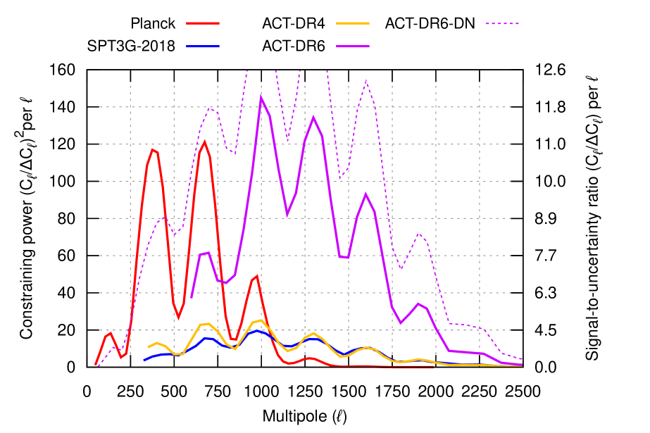
This paper is one of a series presenting ACT Data Release 6 (DR6), which represents a substantial increase in sensitivity compared to our previous data releases and define the state of the art for in T and in E (see figure 2 and Louis et al., 2025). This paper focuses on ACT’s multifrequency maps of the CMB and the microwave sky. Other papers present the angular power spectra and fit to CDM (Louis et al., 2025), and extensions to CDM (Calabrese et al., 2025). See section 6 and figure 21 for more details and other DR6 papers.
ACT was a 6-meter off-axis Gregorian telescope, located at 5190 meters altitude in the Parque Astronómico Atacama in Chile’s Atacama Desert, with access to over half the celestial sphere at arcminute resolution. ACT’s most recent data release was DR5 (Naess et al., 2020), but this was an interim data release focused on small-scale science, and was not sufficiently calibrated for, say, power spectrum analysis. The previous full ACT data release was DR4, which used data collected from 2013 to 2016. Since then ACT upgraded to the AdvancedACT222Also known as Advanced ACTPol. camera and conducted a 2017–2022 survey, the results of which we now release as DR6.
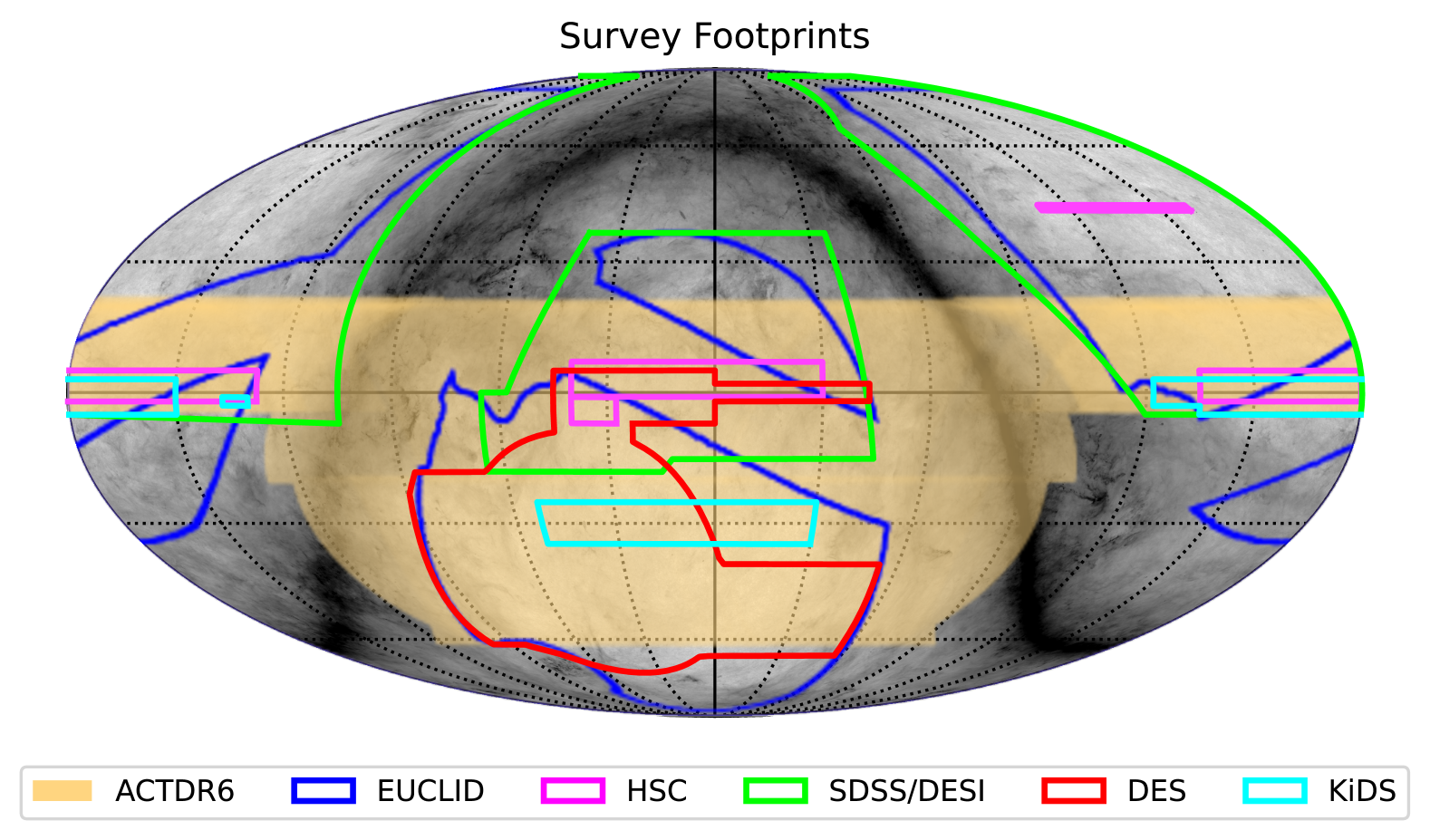
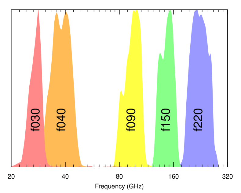
This is the largest step up in data volume of any full ACT data release, with 6–10 times333It is 6 for night-time observations, 10 when including lower quality day-time observations. as much data as DR4. DR6 covers about 45% of the sky with (see figure 1) relatively even depth, unlike DR4 where most of the time was spent observing small patches. The AdvancedACT camera also expanded ACT’s frequency coverage from two bands, f090 (77 – 112 GHz) and f150 (124 – 172 GHz) to five: f030 (21 – 32 GHz), f040 (29 – 48 GHz), f090, f150 and f220 (182 – 277 GHz) (see figure 3), though we postpone analysis of f030 and f040 to a future release. Due to differences in systematic effects we do not include DR4 as a subset of DR6, keeping them as independent data sets.
2 Data selection and characterization
2.1 Summary of instrument and observations
The ACT camera consists of three optics tubes (Thornton et al., 2016), each housing a single dichroic polarized array (PA) with a field-of-view on the sky. The PAs are each equipped with feedhorn-coupled AlMn transition edge sensor polarimeters fabricated on 150-mm diameter silicon wafers, and operate at around 100 mK (Crowley et al., 2018; Choi et al., 2018; Li et al., 2021). These arrays use a two-stage superconducting quantum interference device (SQUID) system, specifically designed for time-division multiplexing (Henderson et al., 2016). From 2017 to the end of 2019, ACT operated with two mid-frequency (MF, f090/f150) arrays, PA5 and PA6, and one high-frequency (HF, f150/f220) array, PA4. At the beginning of 2020, the MF array PA6 was replaced by the LF array PA7 (f030/f040).
DR6 is based on 428 TB of data (144 TB compressed; see table 1) collected from 2017-05-05 to 2022-07-02 (excluding PA7). During this 1883 day period we collected 870 days worth of data (46% observing efficiency), of which 828 days (95%) are CMB observations (i.e. not of calibration targets like planets). Of this, 428 (52%) were observed during the night, and 400 (48%) during the day. Day-time data are typically of worse quality due to the Sun’s heat deforming the mirror surface.
| band | arr | ndet | dur | srate | size | disk | ratio |
|---|---|---|---|---|---|---|---|
| N | days | Hz | TB | TB | % | ||
| f090 | PA5 | 852 | 828.0 | 395.25 | 87.7 | 30.5 | 34.8 |
| f090 | PA6 | 852 | 458.7 | 395.25 | 48.6 | 16.5 | 34.1 |
| f150 | PA4 | 1006 | 818.5 | 300.48 | 77.8 | 22.5 | 28.9 |
| f150 | PA5 | 852 | 828.0 | 395.25 | 87.7 | 30.5 | 34.8 |
| f150 | PA6 | 852 | 458.7 | 395.25 | 48.6 | 16.5 | 34.1 |
| f220 | PA4 | 1006 | 818.5 | 300.48 | 77.8 | 22.5 | 28.9 |
2.2 Data selection
| full | night | day | ||||||||
|---|---|---|---|---|---|---|---|---|---|---|
| band | arr | obs | sel | % | obs | sel | % | obs | sel | % |
| f090 | PA5 | 828.0 | 537.1 | 64.9 | 428.1 | 335.4 | 78.3 | 399.9 | 201.7 | 50.4 |
| f090 | PA6 | 458.7 | 308.5 | 67.3 | 237.3 | 192.3 | 81.1 | 221.4 | 116.2 | 52.5 |
| f150 | PA4 | 818.5 | 502.8 | 61.4 | 422.9 | 310.5 | 73.4 | 395.7 | 192.3 | 48.6 |
| f150 | PA5 | 828.0 | 532.6 | 64.3 | 428.1 | 333.4 | 77.9 | 399.9 | 199.2 | 49.8 |
| f150 | PA6 | 458.7 | 300.4 | 65.5 | 237.3 | 187.5 | 79.0 | 221.4 | 112.9 | 51.0 |
| f220 | PA4 | 818.5 | 471.9 | 57.7 | 422.9 | 294.2 | 69.6 | 395.7 | 177.7 | 44.9 |
Our data selection broadly follows the procedures in Aiola et al. (2020), which are described in more detail in Dünner et al. (2013). It proceeds in three stages. First, data for each array is split into chunks typically 11 minutes long called TODs,444TOD is short for Time-Ordered Data. A typical TOD consists of around 260k samples each for 700 selected detectors, for a total of around 200 million samples. and each of these is accepted or rejected as a whole based on levels of precipitable water vapor (PWV) or the number of well-performing detectors (appendix A.3); or if the day-time beam deformation gets too large (appendix D). The fraction of observing time that passes this selection for each data set is shown in table 2, but typically 75% of the TODs are accepted during the night, and 50% during the day.
| night | day | |||||||||
|---|---|---|---|---|---|---|---|---|---|---|
| band | arr | raw | alive | sel | samp | sel | samp | |||
| N | N | % | N | % | % | N | % | % | ||
| f090 | PA5 | 852 | 738 | 87 | 646 | 88 | 99.0 | 618 | 84 | 94.9 |
| f090 | PA6 | 852 | 637 | 75 | 532 | 84 | 99.1 | 520 | 82 | 97.1 |
| f150 | PA4 | 1006 | 475 | 47 | 324 | 68 | 98.9 | 291 | 61 | 95.9 |
| f150 | PA5 | 852 | 745 | 87 | 665 | 89 | 99.2 | 634 | 85 | 96.4 |
| f150 | PA6 | 852 | 651 | 76 | 576 | 89 | 99.0 | 554 | 85 | 97.3 |
| f220 | PA4 | 1006 | 502 | 50 | 341 | 68 | 98.5 | 287 | 57 | 97.0 |
Secondly, individual detectors are cut on a TOD-to-TOD basis, based on metadata availability (e.g., usable bias step555 In a bias step, the voltage bias on a detector is stepped by a few percent approximately every 60 mins to track the responsivities and time constants of the detectors. calibrations) or the detector data’s statistical properties. In particular, we cut detectors which correlate poorly with the common mode in the atmosphere-dominated frequency range 0.01–0.1 Hz; as well as detectors with significant skewness, kurtosis or abnormal RMS in the white-noise dominated frequency range 10–20 Hz. This is described in appendix A.2, and the result is shown in table 3. Around 30% of the detectors are “dead” (never work). Of the remaining 70%, on average around 80% are usable for each individual TOD, for a total average yield of around 55%.
Finally, we also cut sample ranges within each detector timestream that are affected by short glitches from cosmic rays, scan speed anomalies, and samples near scan turnarounds, etc. (appendix A.1). We identify glitches as large spikes in flux that are not coincident with known bright point sources. We also cut samples that see the Sun or Moon in the far sidelobes (appendix C). In most cases around 1% of the samples of the selected detectors are cut during the night and 5% during the day. See table 3 column “samp” for detailed numbers.
2.3 Time Constants
Our detectors are bolometers with non-zero heat capacity, where the energy deposited by photons decays approximately as , with being the detector time constant that dominates the overall “time constant”. In DR6 our time constants are quite fast, with a typical value of ms (see table 4). Uncorrected, this would induce a 0.1%/1%/10% power loss at . When making sky maps we deconvolve each detector’s average time constant as measured from Uranus observations in the period 2017–2019. This ignores small day-to-day fluctuations in the time constants as well as a roughly 0.3 ms increase in the 2020-2022 data. This results in a tiny contribution to the effective beam of the map which is absorbed by our pointing jitter correction (see section 2.7).
| band | arr | 2017–2019 | 2020–2022 |
|---|---|---|---|
| ms | ms | ||
| f090 | PA5 | 0.82 | 1.05 |
| f090 | PA6 | 0.82 | ··· |
| f150 | PA4 | 1.35 | 1.68 |
| f150 | PA5 | 0.77 | 1.06 |
| f150 | PA6 | 0.74 | ··· |
| f220 | PA4 | 1.16 | 1.45 |
2.4 Gain calibration
We calibrate our time-ordered data and sky maps to the usual linearized CMB micro-Kelvin units,666 These are defined as where is the observed spectral radiance at frequency , is the derivative of Planck’s law for Blackbody radiation with resepct to the temperature in Kelvin, and K is the CMB monopole temperature. To first order, these express the local deviation from the monopole temperature, in µK. Unless otherwise stated, all “µK” in this paper are in these linearized CMB units. but data are read out from the detectors in data aquisition units (DAQ units) and must therefore be translated. We do this in two steps: “relative calibration,” which consists of flat fielding and converting from DAQ units to pW, and “absolute calibration”, which uses planet observations to translate from pW to spectral radiance and then µK.
2.4.1 Relative gain calibration
During this analysis we discovered that a high quality relative calibration between detectors, the flat field, is essential for recovering large angular scales in the maps (see section 5.2 and Naess & Louis, 2023). The atmosphere is a beam filling calibrator and is, in this regard, similar to the CMB. This makes it a good candidate for flat-fielding, but some care is required because the atmosphere has a different frequency spectrum than the CMB (Hasselfield et al., 2013), and because it can be confused with ground pickup, magnetic contamination and cryostat temperature drifts.
A method for differentiating atmospheric modes from others is presented in Morris et al. (2024). While the full formalism was developed after the flat fielding was fixed for DR6, the procedure behind the formalism – clearly identifying atmospheric modes for flat fielding – was followed. After identifying atmospheric modes, the optical flat field was measured from each detector’s correlation with the atmosphere in the 0.01–0.1 Hz range, under the assumption that all detectors should see the same atmospheric fluctuations.777This “common mode” assumption limits the maximum accuracy achievable with this method. Spatially separated detectors will see slightly different atmospheric fluctuations, reducing the correlation with the common mode. This reduction will be higher towards the edge of the array. In ACT this effect is subdominant to errors from isolating the common mode in the first place.
In addition to using a cleaner atmospheric signal for flat-fielding, another change from our previous analysis in Aiola et al. (2020) is the use of a monthly average instead of per-TOD flat fields. This sacrifice in time resolution was done to reduce measurement error, and after extensive testing we found a monthly average to be the tradeoff that minimized the low- power loss.
Despite this improvement, we estimate that the flat field is still only accurate to a few percent, and is probably the dominant cause of the low- bias that forces us to discard the TT power spectrum for (see section 5.2). This problem might have been avoided with an external flat field calibrator like the stimulator built into the Simons Observatory Large Aperture Telescope’s primary mirror, provided any unmodeled bandpass mismatches between detectors in the same class are .
Using the bias steps and flat-field, each sample from time-step of detector is calibrated into physical pW units as
| (1) |
Here is the responsivity obtained from the previous bias step, and is the average optical flat field for that month. Bias steps are performed at least once per hour, and involve measuring the detector response as we modulate the detector bias voltage.
2.4.2 Absolute gain calibration
The calibration from pW to CMB temperature fluctuation units in µK is done as in DR4, using observations of Uranus. Uranus is a point source for ACT, so its observed profile lets us determine the instrument beam, and its amplitude and beam area determine the calibration when compared to measurements from Planck. Planck, in turn, has calibrated Uranus’ flux to 1% accuracy using the CMB dipole (Planck Collaboration, 2017), in agreement with earlier measurements from WMAP (Weiland et al., 2011, 3% accuracy at 94 GHz).
The instrument gain depends on the loading, which is mostly determined by how much water vapor we look through. We use multiple Uranus observations at different elevations (el) and weather conditions to fit a linear model of gain as a function of . This model is then used to predict the calibration for each individual TOD. The gain is typically around 10 K/pW.
Due to scatter in the gain-loading relation as well as the mismatch between the beam-filling CMB and the point-like Uranus, this calibration is only good to around 1–4% accuracy, depending on the band. After the maps have been made, we therefore perform a final calibration against Planck using the CMB perturbations themselves, as described in Louis et al. (2025) and section 3.10.
2.5 Polarization angles
Another critical calibration parameter is the detector polarization angle, which describes the rotation of the polarization signal in the maps relative to the sky. This angle has three components:
-
1.
The orientation of the orthogonal pick-up antennas on the wafer. From the fabrication process, this is known to .
-
2.
The orientation of the wafer in the focal plane. This is relatively straightforward to measure because it also results in a rotation of the individual detectors’ pointing on the sky. Using Uranus observations, we determine the average effect of this rotation in the DR6 maps to be -0.119/-0.019/-0.028 0.011/0.004/0.004 degrees for PA4/PA5/PA6.
-
3.
Polarization rotation from the optical system. The alignment of optical elements with respect to the detectors and the position of the ACT camera relative to the telescope reflectors can introduce a source of rotation of the entire detector array when projected onto the sky. As with DR4 (Choi et al., 2020), we model the full optical system, reflectors plus lenses, and quantify the polarization angle rotation across the focal plane using Optics Studio CODEV. We find a smoothly changing 1.2/1.2/0.4 degree change across PA4/PA5/PA6 as one moves away from the optical angle (Koopman et al., 2016), which is taken into account in our mapmaking. The systematic uncertainty on these numbers is (Murphy et al., 2024).
The total polarization angle systematic uncertainty is therefore , shared between all detectors in each array.
2.6 Pointing corrections
The general principle of the pointing correction is the same as for DR4: an initial pointing model constructed from planet observations gives us a blind pointing accuracy of around an arcminute. This is comparable to our beam size and therefore unacceptably large, so we construct a per-TOD correction using observed positions of bright point sources with known coordinates from external catalogs.
DR6 uses constant elevation scans like DR4, but the typical scanning amplitude has increased from to peak-to-peak, meaning that each TOD covers a much wider azimuth range. During the course of the DR6 analysis we discovered that there can be an up to 0.5′ pointing error difference between the left and right ends of our largest azimuth scans. This led us to introduce a time-dependent azimuth slope in our pointing model. We also modified how the fit is done from an expensive direct time-domain fit to a cheaper and higher time-resolution fit based on short exposure maps (“depth-1 maps”, see appendix E for details).
Despite these improvements in the model, the average pointing jitter in DR6, as inferred from the difference between the beam inferred from point sources in the CMB maps and that measured from individual planet observations, is , around 30% worse than DR4. We interpret this as being due to the more challenging wide scans in DR6. In any case, our pointing jitter represents just a 2% increase in the effective beam FWHM, and is included as part of our beam model.
2.7 Beams and polarized beam leakage
The instrumental beam for the nighttime observations is determined in a similar way as was done for DR4 (Lungu et al., 2022). Details of the DR6 beam estimation are described in a dedicated paper (Duivenvoorden et al., in prep). Here, we provide a summary of the methodology and the available beam products.
Our primary beam estimate is based on dedicated observations of Uranus that were taken throughout the observing seasons. To avoid the large-scale power loss described in section 3, we use a custom mapmaking algorithm which eliminates this bias within 12′ from the planet location (Lungu et al., 2022). If not corrected, this bias would manifest as negative “bowling” around the source, as well as a stronger stripe in the scanning direction. While faint relative to the central peak of the beam, this would be enough to wash out the signal in the wings of the beam.888See section 3.3.4 for how we avoid this effect around bright point sources in the map.
A radial profile is computed from each Uranus map. A parameterized model for the radial profile is then jointly fit to all profiles for a given season. The resulting profiles are largely consistent between the seasons, with the exception of the 2017 observing season (s17), which deviates from the later seasons due to a minor refocusing of the telescope at the start of s18. The radial profiles are converted to a harmonic profile using a Legendre polynomial transform and corrected for the non-zero solid angle of Uranus, the pixel window of the maps and other small biases, as described in Lungu et al. (2022). Because the sky maps combine all seasons into four split maps made from disjoint observations, the per-season harmonic profiles are linearly transformed into per-split profiles. The weights for this transformation are estimated from the statistical contribution of each season to each of the splits. At this point of the analysis, the beams describe the angular response to a source with the SED of Uranus and have not yet been corrected for any beam-altering effects present in the sky maps.
To color-correct the Uranus beams to beams appropriate for the CMB and other sky components, the frequency-dependence of the beam is inferred using a model of the beam based on physical optics simulations. The parameters of the model are found by integrating the frequency-dependent beam model weighted by the Uranus SED over the instrumental passband and finding the parameter values that best describe the observed Uranus profile. From the inferred frequency-dependent beam, the beams appropriate for other sky components are then derived. The correction for pointing jitter and other small beam-altering effects that might be present in the sky maps is computed by finding the best-fitting symmetric Gaussian convolution kernel that describes the difference between the beam derived from Uranus to a set of bright point sources in the sky maps.
Unlike the DR4 case (Lungu et al., 2022), we also make a set of secondary planet maps using the standard CMB mapmaker (section 3), to study the effect of mapmaker nonideality on the beam. In principle this could be used to measure the precise shape of the low- power loss, but in practice even Uranus is not bright enough to get a usable measurement at these multipoles in the presence of atmospheric noise.999It might be possible to make it work with a brighter source like Saturn, but here the challenge is saturation of the central peak. We therefore estimate the low- power loss using the CMB itself (section 5.2). However, the secondary planet maps are still useful for studying temperature-to-polarization (TP) leakage. This has two advantages compared to the primary planet maps.
-
1.
It captures any TP leakage introduced by the mapmaker itself
-
2.
It is not limited to , allowing us to capture where power spectrum null tests indicate significant TP leakage.
Both types of planet maps are analysed further in Duivenvoorden et al. (in prep), where we use them to build a beam model including TP leakage. The effective map beams have a FWHM of 1.42/2.07/1.01 arcminutes at f090/f150/f220 with individual detector arrays in the same band deviating from these averages by arcmin. When excluding the near sidelobes (see appendix B), around 0.01% and 0.002% of the total intensity beam power101010Defined as leaks into E and B respectively.
2.8 Data sensitivity
During DR6, ACT’s passbands f090/f150/f220 had an average instantaneous night-time sensitivity of 8.4/8.9/43 K respectively, giving a combined sensitivity of 6.1 K.111111The day-time numbers are about 5% higher. The total inverse variance (weight) is 0.95/nK2 (night: 0.61/nK2, day: 0.34/nK2). Hence, DR6 has almost 10x the weight of DR4’s 0.096/nK2 (6.4x for night-only). See table 5 and table 6 for more details.
| Full | Night | Day | |||||||||||
| Band | Arr | Weight | Dtime | Dsens | Asens | Weight | Dtime | Dsens | Asens | Weight | Dtime | Dsens | Asens |
| years | K | K | years | K | K | years | K | K | |||||
| f090 | PA5 | 0.285 | 934 | 321 | 12.8 | 0.184 | 593 | 319 | 12.6 | 0.101 | 342 | 326 | 13.1 |
| f090 | PA6 | 0.200 | 446 | 266 | 11.6 | 0.128 | 281 | 263 | 11.4 | 0.072 | 166 | 270 | 11.8 |
| f150 | PA4 | 0.113 | 429 | 346 | 19.6 | 0.073 | 276 | 345 | 19.1 | 0.040 | 153 | 349 | 20.5 |
| f150 | PA5 | 0.196 | 953 | 392 | 15.3 | 0.127 | 608 | 389 | 15.1 | 0.069 | 346 | 399 | 15.8 |
| f150 | PA6 | 0.135 | 468 | 331 | 13.9 | 0.088 | 296 | 327 | 13.6 | 0.047 | 172 | 338 | 14.3 |
| f220 | PA4 | 0.0212 | 415 | 785 | 43.8 | 0.0140 | 275 | 788 | 42.6 | 0.0072 | 140 | 782 | 46.1 |
| Full | Night | Day | ||||
|---|---|---|---|---|---|---|
| Band | Weight | Sens | Weight | Sens | Weight | Sens |
| K | K | K | ||||
| f090 | 0.485 | 8.6 | 0.311 | 8.4 | 0.173 | 8.8 |
| f150 | 0.444 | 9.1 | 0.288 | 8.9 | 0.156 | 9.4 |
| f220 | 0.0212 | 43.8 | 0.0140 | 42.6 | 0.0072 | 46.1 |
| total | 0.949 | 6.2 | 0.613 | 6.1 | 0.336 | 6.4 |
3 Mapmaking
We recover images of the sky from the time-ordered data using the same general framework as set out in Dünner et al. (2013) and used in DR2 (Dünner et al., 2013), DR3 (Naess et al., 2014), and DR4 (Aiola et al., 2020). We summarize this below while pointing out differences.
3.1 Data preparation
We prepare each TOD for mapmaking by
-
1.
Dividing out the instrumental gain.
-
2.
Gapfilling glitches to avoid numerical issues from very high invalid values, and to avoid having them impact the noise model. We gapfill by estimating a detector-detector covariance matrix, and for each sample use this to predict the value of a cut detector given the uncut ones. If all are cut, we simply gapfill using a linear trend. Not all samples that do not pass our data selection are gapfilled – only those flagged as glitches since these are the ones at risk of having extreme values. Since only cut regions are gapfilled, they do not enter into the maps, but they do slightly affect the noise model.
-
3.
De-sloping each detector by subtracting a linear trend from the average of the first 8 samples to the last 8 samples. This is done to make the TOD more Fourier-amenable by reducing the implied discontinuity between the end and the start of the TOD.
-
4.
Deconvolving the instrumental antialiasing filter and the detector time constants.
-
5.
For all but the last mapmaking pass (see section 3.4), Fourier-downsample the TOD to reduce the number of samples and greatly speed up the mapmaking.121212Fourier downsampling reduces the sample rate by simply truncating in Fourier space. To go from samples to samples, one would discard samples above the new Nyquist limit: irfft(rfft(arr)[:m//2+1]). This method preserves power up to the new Nyquist limit while eliminating aliasing, unlike simple averaging of groups of samples which suffers from both aliasing and high-frequency power loss.
-
6.
Reducing to 32-bit float precision to save memory and improve speed. This is enough to handle a per-sample signal-to-noise ratio of , which is more than enough for our noise-dominated TOD. Tests have shown that we end up with the same maps if we use 64-bit precision.
- 7.
Unlike DR4, we no longer perform ground subtraction in time domain. This was not effective enough to avoid the need for map-space filtering during power spectrum estimation, and required expensive time-domain simulations to characterize. In DR6 we leave the ground pickup in the maps because we find it easier to characterize and subtract there.
3.2 Noise model
A noise model is needed to down-weight noisier parts of the data when projecting it onto the sky. Without noise weighting,131313 Or similar techniques that fill the same role in other mapmaking approaches, e.g. high-pass filtering for filter+bin mapmaking or baseline deprojection for destriping. the presence of atmospheric noise would make it impossible to map the CMB from the ground. We use a similar noise model as in Dünner et al. (2013); Naess et al. (2014); Aiola et al. (2020). This models the Fourier-modes of the TOD as being independent, but assumes correlations between individual detectors:
| (2) |
where tells which of around 60 non-equispaced Fourier-bins contains the frequency , and and are detector indices. The matrix represents the part of the noise power that’s uncorrelated between detectors. The matrix contains noise eigenvectors (labeled with ) built as follows. We select eigenvectors with at least 16 times the amplitude of the median eigenvalue from both the atmosphere-dominated frequency range 0.25–4.0 Hz and the instrumental noise-dominated frequency range 4.0–-200 Hz. This typically results in around 10 modes being selected. represents the power of each of these modes for each frequency bin, .
Measuring the noise model from the data itself biases the signal low, since cases where the noise partially cancels the signal appears lower-variance than cases where the noise is in phase with the signal. Overall signal-cancelling noise is therefore given higher weight. We avoid this effect by using multi-pass mapmaking, where the signal estimate from a previous mapmaking pass is subtracted before the noise model is estimated.
3.3 Data model
We model the calibrated time-ordered data for sample of detector as a linear function of a static sky ,
| (3) |
Here is the value of the Stokes parameter at pixel (in units of ), and is Gaussian noise with covariance . represents the contamination in the cut samples, which must be included in the equation system to avoid biasing the results; while represents the model errors in areas with very high contrast, such as near bright point sources. The pointing matrix , the cut mapping and the model error mapping are the response of the data to , and respectively. See sections 3.3.2, 3.3.3 and 3.3.4 for these. We can write the data model in matrix form as
| (4) |
which has the maximum-posterior solution
| (5) |
where is a prior that resolves degeneracies between and (see section 3.3.4). For ACT this is a equation system that must be solved using iterative methods like Preconditioned Conjugate Gradients (CG).
3.3.1 Pixelization
We represent the sky map using a Plate Carrée projection in equatorial coordinates, pixelized with pixels of size covering and . The north and south pole are not included in the maps to avoid wasting space, but would have half-integer declination pixel coordinates, making the maps compatible with Fejer’s first integration rule (Waldvogel, 2006), allowing for efficient “map2alm” inverse spherical harmonics transformations.141414If is the matrix of spherical harmonics basis functions, representing the “alm2map” transform, then the inverse , where is a quadrature weight matrix. The half-integer declination pixel coordinates for the poles ensures that can be evaluated efficiently. These details are irrelevant for the “alm2map” transformation.
This is a change from ACT DR4, where we instead used whole-integer declination pixel coordinates, corresponding to the Clenshaw-Curtis integration rule (Waldvogel, 2006). Clenshaw-Curtis pixelization has the disadvantage that it is not robust to simple resolution downgrading. For example, the simplest way to halve the resolution of a map is to replace each block of pixels with a single new pixel with the average of their values. Under this operation, a Fejer-1 map stays a Fejer-1 map, but a Clenshaw-Curtis map ends up with quarter-integer coordinates for the poles. No integration weights for such a map are available in the DUCC spherical harmonics transform library we use (Reinecke, 2020), nor for other commonly used ones like its predecessor libsharp (Reinecke & Seljebotn, 2013).
The upshot of this is that the DR6 pixelization has a half-pixel declination shift compared to DR4, and that, unlike DR4, DR6 maps can still be inverse spherical harmonics transformed after simple downgrading.
3.3.2 Pointing matrix
The standard practice is to use a nearest-neighbor model for the instrument response , meaning that the value in each sample is simply read off from the nearest pixel, without any interpolation, and this is also what we did in DR4. In practice this means that if the sample with index has nearest pixel , then
| (6) |
where is the Kronecker-delta and is the orientation of the direction of polarization sensitivity on the sky for detector at sample , which is used to handle the spin-2 nature of the Stokes Q and U parameters. This method is popular because it results in being extremely sparse and efficient, with each sample only needing to concern itself with a single pixel, but the cost of this is that we model our data as a set of sudden jumps in value as one moves from one pixel to the next.
However, during the DR6 analysis we discovered that despite a nearest-neighbor only being an inaccurate description of the data at sub-pixel scales (, ), its use can result in bias in the angular power spectrum at any scale where the noise model is highly correlated (see section 5.2). For a ground-based microwave telescope like ACT the atmosphere causes large amounts of unpolarized correlated noise at low , and the result is that the unphysical sub-pixel treatment in a nearest-neighbor propagates into a large power loss in the low- TT power spectrum. This unintuitive effect is described in detail in Naess & Louis (2023).
The most obvious solution for sub-pixel errors is to simply reduce the pixel size, but this is not practical. Sub-pixel bias is first order in the pixel size, so to reduce the bias to one would need 100 times as many pixels. Not only would this be far too big, it would also spread out the samples too thinly, leaving many pixels unhit. A much better solution is to switch to a bilinear pointing matrix, which makes the errors second order in the pixel size.
| (7) |
where and are the full (not rounded) x and y pixel coordinate for sample , indicates rounding down, and and similarly for . The cost of this approach is that each sample now touches four pixels rather than one, but we found that the overall runtime increase was around 50% rather than the 300% one might fear.
Bilinear mapmaking produces a different pixel window than nearest neighbor mapmaking (see figure 16 of Naess & Louis, 2023), but to avoid requiring changes to code that uses our maps, we reconvolve them to the standard nearest neighbor pixel window.
3.3.3 Cut sample model
We do not want the values of the samples that do not pass our data selection criteria to affect our sky map, but we cannot simply skip them in the likelihood because our noise model is Fourier-based, and the Fast Fourier Transform requires the samples to be equi-spaced. On the other hand, using the values as they are would contaminate the map, and replacing them with a fixed value like zero would bias it. The standard solution to this problem is to include the values of the cut samples as degrees of freedom in the likelihood, and this is what the vector in equation 4 represents.
In the simplest form, we allocate one degree of freedom per cut sample, and use these values instead of the ones read off from the map in the data model (equation 3). This is implemented by zeroing out the corresponding rows in , with these rows becoming the only non-zero rows in . This is illustrated for a toy example with a single detector scanning across 4 pixels with constant speed over the course of 7 samples, with samples 3, 4 and 7 being cut151515 The entries in occur when a sample hits halfway between two pixels.
| (8) |
To save memory, we implement a somewhat more complicated version of this where our degrees of freedom represent the Legendre polynomial coefficients of the cut samples instead of the one-to-one mapping shown above. For cuts of length up to 1/3/6/20 samples we allocate 1/2/3/4 degrees of freedom, and beyond that we use the nearest integer to where is the duration of the cut in seconds.161616There are typically around 100 samples per second in the first two mapmaking passes and 400 samples per second in the final pass.
The general method was suggested by Patanchon et al. (2008) and used in DR2–DR4, but was not described in as much detail there.
3.3.4 Model error mitigation in high-contrast areas
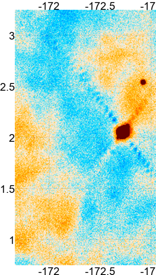
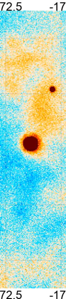
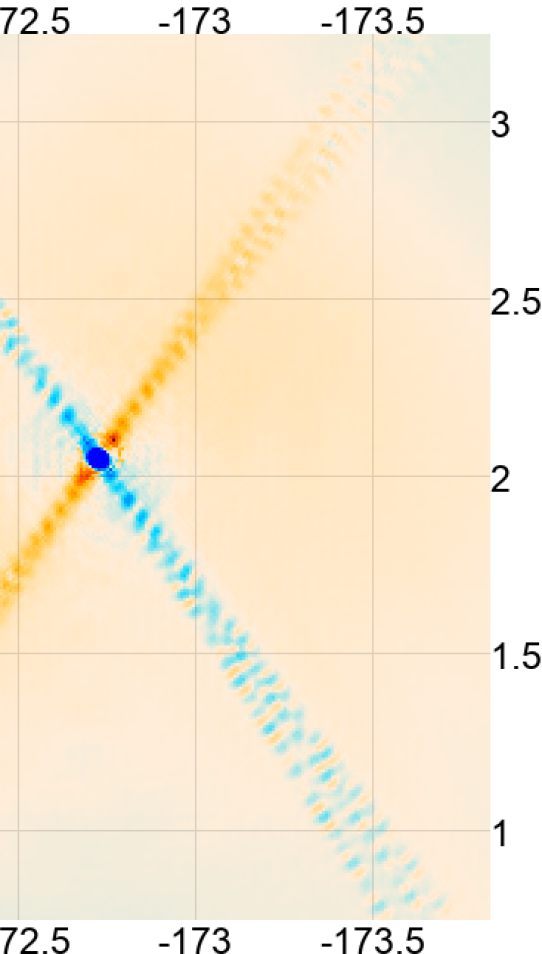
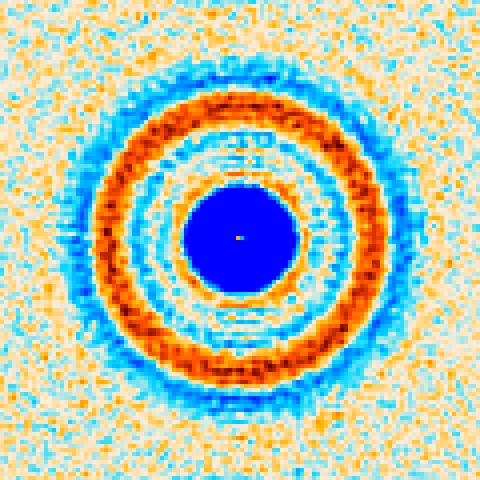
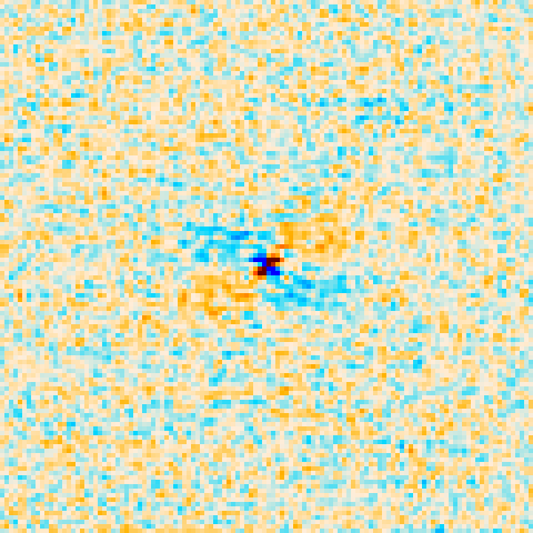
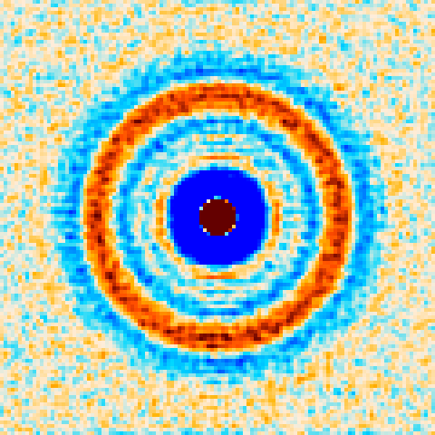
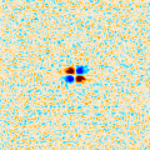
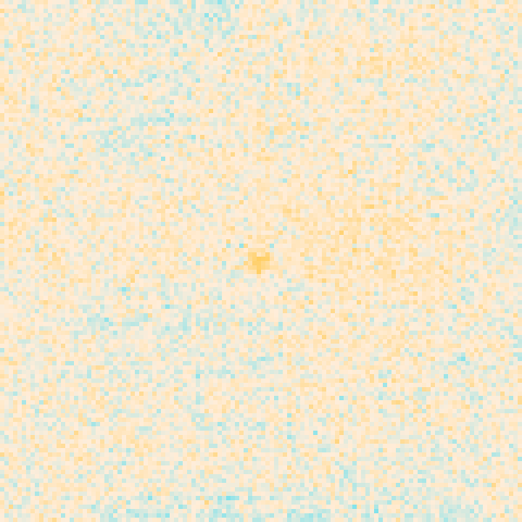
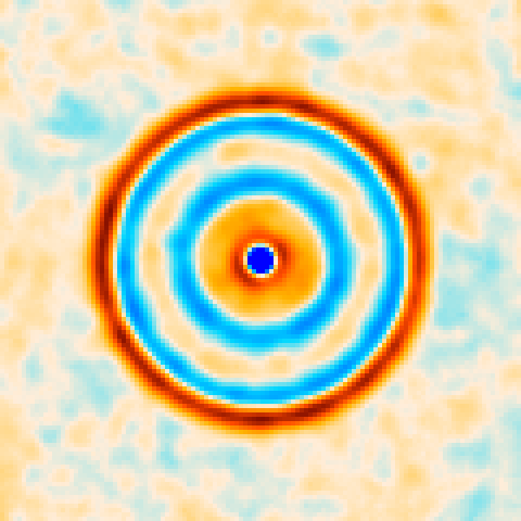
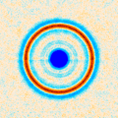
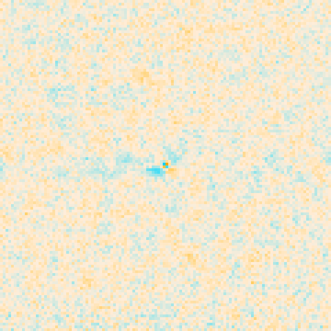
Even with a bilinear pointing matrix the data model is never 100% accurate. Tiny sub-pixel errors remain, as well as unmodeled pointing jitter and gain fluctuations. Furthermore, the sky itself is variable, especially compact objects like quasars. As described in Naess & Louis (2023), mismatch between the model and data can manifest as a loss of power at large scale, effectively introducing a slight high-pass filter in the mapmaking. This is undesirable as a whole but especially problematic near bright objects, where it manifests as thin, X-shaped artifacts extending several degrees away with an amplitude of of the peak (Næss, 2019). An example of this is shown in figure 4.
| Without | With | Difference |
|---|---|---|
 |
 |
 |
To avoid needing to mask out large areas around each bright source (or omitting them from the map altogether) we instead completely eliminate model error for these objects by allocating an extra degree of freedom for every sample that hits them. This gives the model the freedom to absorb arbitrary data behavior in this region. We implement this using the vector and the corresponding response matrix which works very similarly to the cuts matrix, , (section 3.3.3), with two main differences
-
1.
We use one degree of freedom per selected sample, not a Legendre polynomial.
-
2.
We do not remove the corresponding rows from the pointing matrix .
The last point makes eq. 5 underdetermined: it’s ambiguous whether the signal should go into the pixels near the objects or into . We resolve this using the prior in the equation, which takes the form:
| (9) |
where the diagonal matrix is the uncorrelated part of the inverse noise variance predicted by for each sample in ,171717 gives the prior the same units as and ensures that these terms will have a consistent relative strength regardless of each TOD’s length or noise level. and is an edge weighting factor that interpolates logarithmically from 10 for samples at the edge of each region to 0.01 for samples 2 arcminutes away from the edge.181818 The edge taper avoids noise discontinuities at the edge of the region.
The effect of this prior is to give a mild preference for putting the signal in instead of . Hence, anything that could be represented by will end up there, while what cannot (the model errors) end up in .
One might wonder if this technique could be used to eliminate model errors everywhere in the map, but this would not work. Aside from needing a dauntingly large , the very act of solving for so many extra degrees of freedom degrades the noise properties of the map by spreading the data too thin. In the absence of the prior there would be no averaging at all, and even with it there’s a tradeoff between bias and optimality. The method performs best when restricted to areas small enough that the correlated noise is still well constrained by the surroundings, and bright enough that the loss of optimality is not noticeable.
For the DR6 maps, we use this method for pixels that fall within the mask srcsamp_mask.fits (see table 9), which covers areas within 3 arcminutes from a point source detected at mJy at f090, or which is within 3 arcminutes of an area where is above its 99.99%-quantile, where is the Planck 545 GHz map. This captures the brightest 207 point sources in the map, as well as the areas of the Galaxy with the brightest dust emission like the galactic center and the Orion nebula. All in all, 51060 pixels (11.55 square degrees, 0.06% of our sky coverage) are given this treatment.
3.4 Multipass mapmaking
There are several reasons why it’s useful to split the mapmaking process into multiple passes.
-
1.
As noted in 3.2 we build the noise model from the data itself, but this contains the sky signal we want to measure. Using a noise model contaminated by the sky signal to weight the data results in a biased map. We can avoid this by subtracting an estimate of the signal before building the noise model, but this requires us to already have made a map.
-
2.
Given an estimate of the sky, we can perform a cheap first-order correction for the polarized sidelobes.191919Since these sidelobes are an effect, the effect of ignoring higher orders is a negligible .
-
3.
Mapmaking can be greatly sped up by downsampling the time-ordered data, but this introduces a small loss of power at high . However, high- converges in just a few Conjugate Gradients steps, so this can be fixed by running a few CG steps with no downsampling at the end.
With this in mind, we make maps in three passes, with pass 2 and 3 continuing from the result of the previous pass202020For now the cut and source sub-sampling degrees of freedom are solved from scratch in each pass. While not optimal, these degrees of freedom are not bottlenecks for the CG convergence. while using it to debias the noise model and subtract the polarized sidelobes. We use 300 CG steps with 4x downsampling for the first two passes; and 30 CG steps with no downsampling for the last pass.
3.5 Noise splits
Like in DR4, we split our data into noise splits. Briefly, each array-band combination for each data set is split into 4 independent subsets (typically, see table 9) and mapped separately. These give us views of the sky with the same signal but independent noise realizations, allowing us to eliminate noise bias in our power spectrum estimation by using cross-only estimators. See Louis et al. (2025) for details on the power spectrum estimation.
3.6 Null test maps
Aside from the normal sky map, we also make a special set of null test maps. The purpose of these is to maximize the effect of various types of systematics we suspect could be in the data, and hence maximize our ability to detect these. A disadvantage of maximum-likelihood mapmaking is that making such null maps is relatively expensive, so we limited ourselves to the most well-motivated tests.
The actual null tests performed using these maps are detailed in Louis et al. (2025).
3.6.1 PWV split
The amount of precipitable water vapor affects the opacity of the atmosphere, and therefore both the loading and the amount of correlated noise. Loading can affect gain and saturation, while more correlated noise can increase the low- power loss. To compensate for lower sensitivity at high values of PWV, we split the TODs into two somewhat uneven subsets: with 33% of the TODs and with 67% of the TODs.
3.6.2 Elevation split
The main job of the elevation split is to test for ground pickup, which is strongly elevation-dependent. To a lesser extent, this test also tests for loading effects, as lower elevations have longer atmospheric sightlines. The DR6 scans happened at 3 discrete boresight elevations: , and , each with one third of the data. We mapped these separately for this test.
3.6.3 Time split
Some telescope systematics could change over long timescales. For example, we know that the overall telescope focus changed slightly in May 2018 when the secondary mirror axes were disabled. A time split makes us maximally sensitive to long-term changes in telescope behavior like this. For the purpose of this test we split the TODs into two subsets: one from before February 2019 and one after. This relatively uneven split was driven by the wish to not dilute the known focus change in 2018 by too much.
3.6.4 Inner-outer split
Unlike the other null tests, this did not split the data by TOD, but by detector. Each detector array has its own optics tube, and we expect optical properties to change mainly as a function of the distance from the tube’s central axis. We therefore split the detectors into an inner and outer subset based on this distance. The cutoff radius was chosen to give the two subsets equal sensitivity, but in practice this was close to a 50-50 split.
3.7 Short-timescale ‘Depth-1’ maps
ACT observes the sky by performing broad-amplitude azimuth scans with a typical peak-to-peak amplitude of 60 at constant elevation while the sky drifts past. These scans typically last from 0.5 to 7 hours and cover 100 to 2900 square degrees to a typical depth of around 250 µK′ (roughly 25 mJy) before repointing to scan a different area of the sky. See table 7 for details. To explore the time-variable sky we map each scan by itself in a special mapmaking run. We call these ‘depth-1’ maps because they are a single scan deep, though ‘single scan maps’ might have been more descriptive. The maps were made with the standard maximum-likelihood framework, but since only small scales are time-variable on human-relevant timescales, only a single pass with 100 CG steps was used. The number of steps was driven by the need for the cuts degrees of freedom to converge. Had it not been for this, 10 CG steps would probably have sufficed.
Due to the large number of these maps (around 30k map-sets, 190k files total; see table 9) and the expense of updating them, these maps have some caveats that do not apply to our other maps, including calibration drifts and occasional artifacts and pointing outliers, as well as deviations from our normal beam shape during the subset of observations that happen during the day. See table 11 for details.
| band | arr | maps | depth | depth |
|---|---|---|---|---|
| N | µK′ | mJy | ||
| f090 | PA5 | 5519 | 280 | 25 |
| f090 | PA6 | 3145 | 230 | 22 |
| f150 | PA4 | 5339 | 410 | 48 |
| f150 | PA5 | 5474 | 310 | 32 |
| f150 | PA6 | 3107 | 260 | 29 |
| f220 | PA4 | 4928 | 780 | 78 |
3.8 Matched filtered maps
We also produce a set of matched filtered versions of the depth-1 maps to make point source analysis easier. The matched filter map is the pixel-by-pixel answer to the question: “What is the maximum-likelihood flux density for a point source at the center of this pixel, assuming the rest of the map has no signal?” The answer is
| (10) |
where is the depth-1 map after converting it from µK CMB to mJy/sr assuming a frequency of 98/150/220 GHz for the f090/f150/f220 bands,212121 Precision analysis will probably need to rescale these units to the actual effective bandcenter based on the bandpass and object’s spectral tilt. is the pixel-pixel matrix of , is the beam covariance matrix, and the division is done pixel-by-pixel. We label the numerator and denominator of this estimator and respectively. These turn out to be more useful to distribute than itself, because they are both linear in the data and therefore easy to coadd over whatever timescale the user is interested in (, ). The flux and uncertainty are then recovered as , .
To approximate (which is not actually available due to being prohibitively expensive to build for maps of this size) we model it as
| (11) |
where is the per-pixel white noise variance, which is diagonal in pixel
space and available from the ivar map, and is diagonal in 2D
Fourier space, and is measured from . This somewhat complicated
model allows us to handle stripy correlated noise and position-dependent depth.
3.9 ILC maps
Coulton et al. (2024) performed component separation of the DR6.01 maps using the Needlet Internal Linear Combination NILC method. We repeat this analysis using the updated DR6.02 maps, with no changes in methodology.
To summarize, we use the NILC method to isolate the blackbody temperature component, which contains the CMB temperature anisotropies and kinetic Sunyaev Zeldovich effect, the blackbody E-mode polarisation component, and a map of the Compton-y effect. The NILC method minimizes the sum of the foreground and noise variance, and in the presence of noise this can leave residual foregrounds at a level comparable to the noise level, or higher in small areas where the noise or foreground properties change more rapidly than the model can account for. To mitigate these foreground residuals we provide variations that explicitly remove known contaminants, at the cost of increased noise. To test the effectiveness of the contaminant removal we provide maps with different assumptions about the contaminant signals. For further details see Coulton et al. (2024).
3.10 Final gain and polarization efficiency correction
After the maps were made, we performed a final calibration against Planck, fitting a per-array gain correction and polarization efficiency. This is described in Louis et al. (2025), and the results are shown in table 8. As indicated in table 9, the maps we release are corrected by these factors (all close to unity), with the exception of the depth-1 maps.
| PA5 | PA6 | PA4 | PA5 | PA6 | PA4 | |
|---|---|---|---|---|---|---|
| f090 | f090 | f150 | f150 | f150 | f220 | |
| gain | 1.0111 | 1.0086 | 1 | 0.9861 | 0.9702 | 1.0435 |
| poleff | 0.9534 | 0.9715 | 1 | 0.9545 | 0.9679 | 0.9074 |
4 DR6 map products
The DR6 map products are summarized in table 9
and its supporting tables 10 and 11. The main
products are the DR6 night-time maps act_dr6.02_std_AA_night (with supporting null
maps) and the Depth-1 maps
act_dr6.02_depth1. We also release a set of DR5-style coadd maps aimed
at visualization and cross-correlation science; see Naess et al. (2020) for
details and caveats with these maps.
For the first time we also release our raw day-time maps. These were
processed the same way as the night-time maps with additional cuts on
Sun sidelobes and beam deformation. Despite this, the beam in these maps
is less well understood than for the night-time maps. Finally, we
release a few miscellaneous maps targeting small areas of the sky.
| Name | Types | Notes | Split | Files | Width | Height | Size | Description |
act_dr6.02_std_AA_night |
msvx | NTPWG0 | 4 | 96 | 43200 | 10320 | 399 | Main DR6 data set |
act_dr6.02_depth1 |
mvti | NTipw dgGH | 1 | 125k | var. | var. | 20000 | Plain Depth-1 maps |
act_dr6.02_depth1 filtered |
pdgfucsH | 1 | 63k | var. | var. | 24000 | Matched filtered Depth-1 maps | |
| Coadd maps | msV | NTp WdGd | 1 | 36 | 43200 | 10320 | 180 | Coadd into single-frequency maps. With/without day-time, with/without DR4, without Planck |
| Planck coadd maps | msV | pWdBd | 1 | 36 | 43200 | 10320 | 180 | As above, but with Planck |
| ILC maps | I | RL | 1 | 3 | 43200 | 10320 | 5 | NILC component separated maps |
| Deprojected ILC maps | d | RL | 1 | 71 | 43200 | 10320 | 118 | NILC maps with explicit deprojection of tSZ/CIB/etc. |
act_dr6.02_null:pwv[12]_AA_night |
msvx | NTPWG | 4 | 192 | 43200 | 10320 | 797 | Night PWV split |
act_dr6.02_null:el[123]_AA_night |
msvx | NTPWG | 4 | 288 | 43200 | 10320 | 1196 | Night elevation split |
act_dr6.02_null:t[12]_AA_night |
msvx | NTPWG | 2 | 96 | 43200 | 10320 | 399 | Night time split |
act_dr6.02_null:inout[12]_AA_night |
msvx | NTPWG | 4 | 192 | 43200 | 10320 | 797 | Night in/out split |
act_dr6.02_std_AA_day |
msvx | NTPWGd | 4 | 96 | 43200 | 10320 | 200 | Wide day survey |
act_dr6.02_std_DN_day |
msvx | NTPWGd | 4 | 96 | 12911 | 2203 | 13 | North day survey |
act_dr6.02_std_DS_day |
msvx | NTPWGd | 4 | 96 | 13726 | 2849 | 17 | South day survey |
act_dr6.02_std_GC_night |
msvx | NTPWGu | 2 | 48 | 1920 | 1560 | 1.3 | Galactic center night |
act_dr6.02_std_BR_night |
msvx | NTPWGu | 2 | 32 | 1080 | 1020 | 0.3 | A399–401 bridge night. No PA6 |
act_dr6.02_std_D5_night |
msvx | NTPWGu | 4 | 96 | 3913 | 1672 | 5.8 | D5 night |
srcsamp_mask.fits |
- | - | 1 | 10800 | 2580 | 0.0026 | Model error mitigation mask. See section 3.3.4 | |
beam_status.txt |
b | - | - | 1 | - | - | 0.025 | Depth-1 beam status |
depth1_index.txt |
j | - | - | 1 | - | - | 0.0032 | Time/pos of each Depth-1 map |
ilc_valid_mask.fits |
M | - | - | 1 | 43200 | 10320 | 0.4 | ILC well tested here |
ilc_inpaint_mask.fits |
M | - | - | 1 | 43200 | 10320 | 0.4 | Strong ILC residuals inpainted here |
| Type | Description |
|---|---|
| m |
map: Sky map with shape (3,height,width) corresponding to the Stokes parameters
I, Q and U, in µK CMB units. The maps have been reconvolved to the standard
nearest-neighbor pixel window.
|
| s |
map_srcfree: Like m, but with all point sources detected at in the full ACT
coadd subtracted. This corresponds to median flux limit of 6.5/8.4/29 mJy
at f090/f150/f220, but the exact limit is position-dependent.
|
| v |
ivar: Inverse variance map with shape (height,width) in units .
Describes the Stokes I noise behavior on small scales, where the noise is
approximately white. Q and U have half this inverse variance.
|
| V |
ivar: Like v, but with all of Stokes I, Q and U present.
|
| x |
xlink: Cross-linking information, with shape (3,height,width).
The three fields in each pixel are given by
.
Here is a pixel index, is a TOD sample that hits , is the white noise
inverse variance in sample , and is the angle between the scanning direction
in sample and the direction towards the celestial north pole. The inverse variance
weighted average of the cosine and sine of the scanning direction is then:
and .
If a part of the sky were hit equally by scans at all
angles, both of these would be zero. On the other hand, an area hit only in a single
direction would have a [cos,sin] vector with length 1.
In general if the quantity
is not close to zero, the crosslinking is poor, so this quantity can be
useful to determine whether to mask pixels.
|
| t |
time: Time map with shape (height,width). The value of each
pixel is the time at which each pixel was hit, in seconds relative to info.t.
Defined as the inverse variance weighted average time of all the samples
that hit each pixel. This represents the middle of the exposure interval
of the pixel. The first/last exposure is typically 1.6 minutes before/after.
|
| i |
info: HDF5 metadata file with fields:
array: The array and band for this file, e.g. “pa5_f090”;
box: The bounding box for the area covered by this map. (2,2)-shaped
array with form ,
where the indices 1 and 2 refer to the bottom-left and top-right corners respectively;
ids: The TOD ids mapped in this map;
pid: Sequential identifier for the scans identified during
the depth-1 mapmaking;
t: Unix time of the start of the scan. The time map is
relative to this;
period: Unix time of start and end of the scan.
profile: -shape array giving
dec and RA coordinates tracing out a representative path for
a single azimuth sweep of the telescope. This can be useful when
modelling the curvature of the stripy noise.
|
rho: Matched filter numerator maps with shape (3,height,width)
corresponding to Stokes I, Q and U, in units of . See section 3.8.
|
|
kappa: Matched filter denominator maps with the same
shape as , in units of .
|
|
| I | ILC: NILC component separated map with shape (height,width). Three components available: Compton-y, CMB blackbody T and CMB blackbody E. These maps were constructed to have a Gaussian beam. See Coulton et al. (2024) for details. |
| d | Deprojected ILC: As above, but with one or more of the cosmic infrared background (CIB), thermal Sunyaev-Zel’Dovich (tSZ), relativistic Sunyaev-Zel’Dovich (rSZ) and their derivatives. |
coarse mask: Quarter-resolution sky mask with shape . One in areas the mask applies to, zero elsewhere. For example, for srcsamp_mask.fits, the mask is one in high-contrast areas where special model error mitigation was used.
|
|
| M |
fine mask: Like the coarse mask, but full resolution.
|
| b |
beam status: Whether the beam passes our beam deformation cuts or not, per TOD. One line per TOD, with columns TOD ID (e.g. 1494463442.1494478197.ar4:f150), start and end unix time (UTC seconds since 1970-01-01 00:00:00, e.g. 1494463441) for the TOD, and the status. The status is 0 if the beam passes the cuts and 1 if it fails. See appendix D. Combine this with the depth-1 time maps to roughly reject observations with bad beams.
|
| j |
depth-1 index: Rough time/position coverage of each Depth-1 map. One line per map, with format time start, time end, RA min, RA max, dec min, dec max, name. Times are Unix time (C time), and coordinates are in degrees. name is e.g. depth1_1494478923_pa5_f090, for which a map, ivar, info, rho and kappa file would be available.
|
| Key | Description |
|---|---|
| N | The maps contain correlated noise with a spectrum with and at f090/f150/f220 total intensity and in polarization. The noise is stripy, with position-dependent amplitude and stripe direction. See section 5.1 and appendix F. |
| T | The maps (except Planck coadd) suffer from an unexpected lack of power at in total intensity which we belive is a form of dilution bias mainly sourced by relative gain errors. See section 5.2 and Næss (2019). |
| i | The depth-1 maps’ CG iteration was stopped early, and only one mapmaking pass was performed, resulting in an additional lack of power for . |
| p | The maps have an effective polarization efficiency of . See section 3.10. |
| P | The maps have been corrected for an effective polarization efficiency of . See section 3.10. |
| 0 | The PA4 f150 maps failed the null tests for the angular power spectrum part of our analysis. They suffer from higher levels of leakage and a larger transfer function than our other maps. Care should be taken when using these for precision analysis, e.g. by checking for consistency with the other, more reliable arrays. |
| w | The maps were built using a nearest neighbor pointing matrix, resulting in a standard sinc pixel window |
| W | The maps were built using a bilinear pointing matrix, but have been reconvolved to a standard sinc pixel window |
| d | The day-time maps have a poorly characterized beam |
| B | The map has a scale-dependent bandpass (around 2-5%) due to combining data from different telescopes. See Naess et al. (2020). |
| g | The maps may be subject to drifts in gain on month-to-year timescales. |
| G | The maps are contaminated by pickup (ground and other sources). This is relatively more important in polarization, and mostly manifests as low- horizontal stripes. See figure 20. |
| f | The flat sky approximation was used locally when building the matched filter, resulting in a flux bias up to 1.5% furthest from the equator (dec = 60) |
| u | Occasional artifacts and temporary changes in noise properties are not captured by the matched filter noise model, resulting in false positives that must be worked around in a transient search |
| c | Curvature in the stripy noise was ignored in the matched filter, making it slightly suboptimal |
| s | Areas near bright sources are contaminated by ringing from the matched filter |
| H |
These maps were not postprocessed for release to add
detailed FITS keywords and convert from the cosmology/HEALPix
polarization convention to the IAU one, due to the large data volume
involved. In practice this means the Stokes U sign is flipped.
(You will not need to worry about this if you only read the maps with
pixell.enmap.read_map. It automatically converts back to the
cosmology convention when reading, if necessary, based on the POLCCONV
FITS entry.)
|
| L | The plain ILC maps and those with one component explicitly deprojected are band-limited at . For two/three deprojected components, this number is reduced to . |
|
full |
|
|---|---|
|
night |
|
| Survey | Area | In DR6 | Of DR6 | Type | Ref | ||
|---|---|---|---|---|---|---|---|
| deg2 | % | deg2 | % | % | |||
| ACT DR6 | 19400 | 47.0 | 19400 | 100.0 | 100.0 | CMB | This work |
| BICEP3 | 1890 | 4.6 | 1510 | 80.0 | 7.8 | CMB | Ade et al. (2022b) |
| SPT-3G | 4400 | 10.7 | 3000 | 69.0 | 15.7 | CMB | Guidi (2022) |
| Planck | 41000 | 100.0 | 19400 | 47.0 | 100.0 | CMB | Planck Collaboration (2020) |
| 4MOST | 22000 | 54.0 | 13600 | 61.0 | 70.0 | Spect. | 4MOST (2024) |
| BOSS | 17600 | 43.0 | 6700 | 38.0 | 35.0 | Spect. | Ahumada et al. (2020) |
| DESI | 14300 | 35.0 | 7400 | 52.0 | 38.0 | Spect. | Hahn et al. (2023) |
| Euclid | 17200 | 42.0 | 8800 | 51.0 | 46.0 | Spect. | Euclid Collaboration et al. (2022) |
| DES | 5300 | 12.7 | 5100 | 96.0 | 26.0 | Photo. | Abbott et al. (2021) |
| HSC | 1500 | 3.6 | 1390 | 92.0 | 7.2 | Photo. | HSC (2021) |
| LSST | 28000 | 68.0 | 17900 | 64.0 | 92.0 | Photo. | LSST (2023) |
| WISE | 41000 | 100.0 | 19400 | 47.0 | 100.0 | Photo. | Wright et al. (2010) |
| EMU | 31000 | 75.0 | 19400 | 62.0 | 100.0 | Radio | Norris (2011) |
| RACS | 34000 | 83.0 | 19400 | 57.0 | 100.0 | Radio | McConnell et al. (2020) |
| VLASS | 34000 | 82.0 | 16400 | 48.0 | 85.0 | Radio | Lacy et al. (2020) |
The DR6 sky coverage and depth is shown in figure 5. We cover for and for RA outside this range. When combining f090, f150 and f220 the typical night-time white noise level is 6-12 K arcmin in total intensity, with f090/f150/f220 being on average 1.41/1.45/6.6 times higher. Adding day-time data improves this by about 20%. The Q and U polarization white noise is times as high.
Intensity
 Polarization
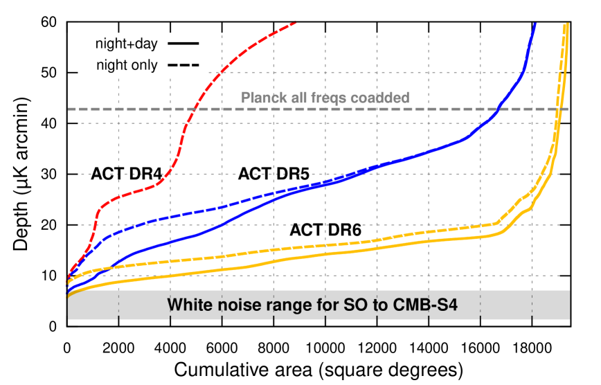
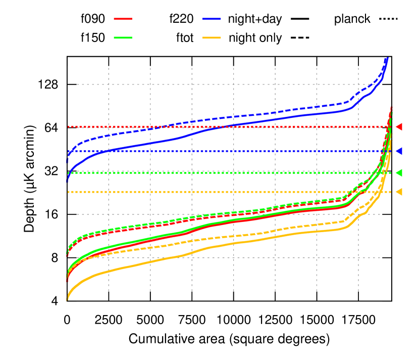
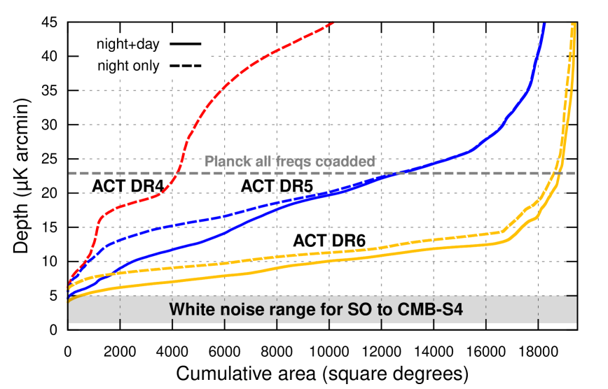
Figure 6 shows the depth distribution and compares it with DR4, DR5 and Planck. DR6 is almost twice as deep (in RMS) as the non-cosmology-calibrated DR5, and more than four times as deep as DR4 (our previous cosmology data release) over most of the sky. The typical DR6 combined depth is K arcmin, and 19 400 square degrees (47% of the sky) are deeper than K arcmin. Figure 7 splits this into our individual bands. The median depth inside the exposed area is 14/14/64/9.6 K arcmin for day+night at f090/f150/f220/ftot and 15/16/74/11 K arcmin for night alone. Here “ftot” refers to the coadd of f090, f150 and f220.
This large sky coverage gives us good overlap with several surveys relevant for cross-correlation studies, as shown in table 12 and figure 1. We cover most of BICEP3, SPT-3G, 4MOST, DES, DESI and LSST, to name a few other surveys.
| Q | 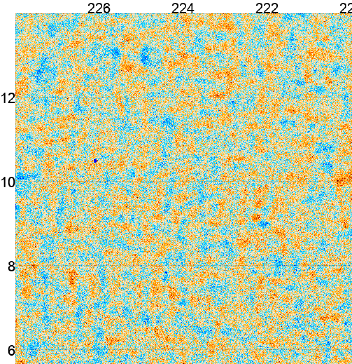 |
 |
U |
| E | 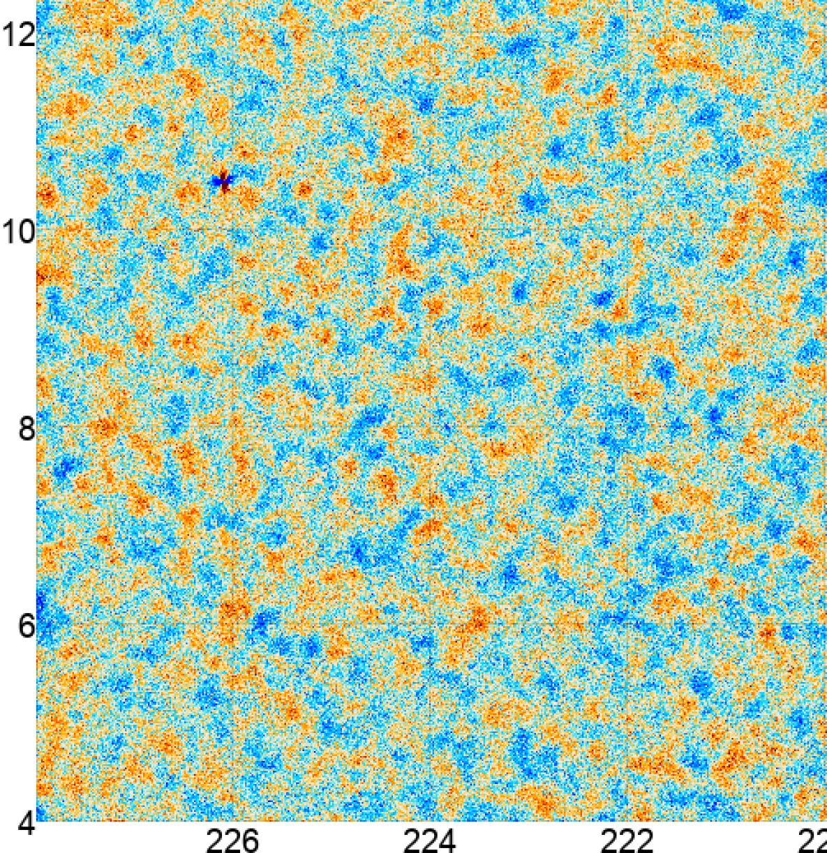 |
 |
B |
|
Planck |
 |
 |
 |
 |
 |
|
ACT |
 |
 |
 |
 |
 |
|
ACT+Planck |
 |
 |
 |
 |
 |
|
Simulation |
 |
 |
 |
 |
 |
|
Planck |
 |
 |
 |
 |
 |
|
ACT |
 |
 |
 |
 |
 |
|
ACT+Planck |
 |
 |
 |
 |
 |
|
Simulation |
 |
 |
 |
 |
 |
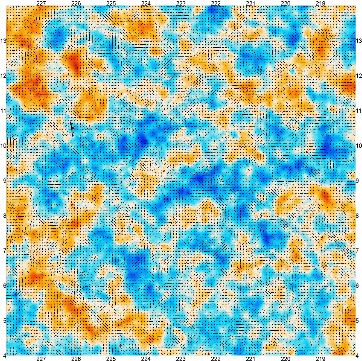
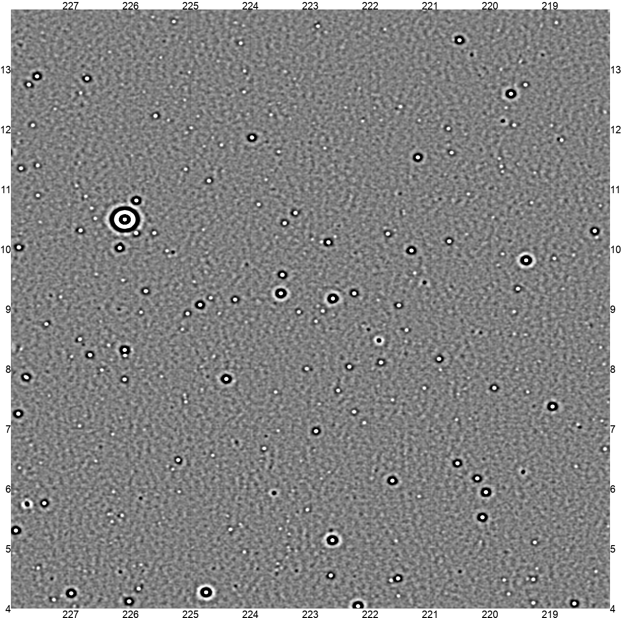
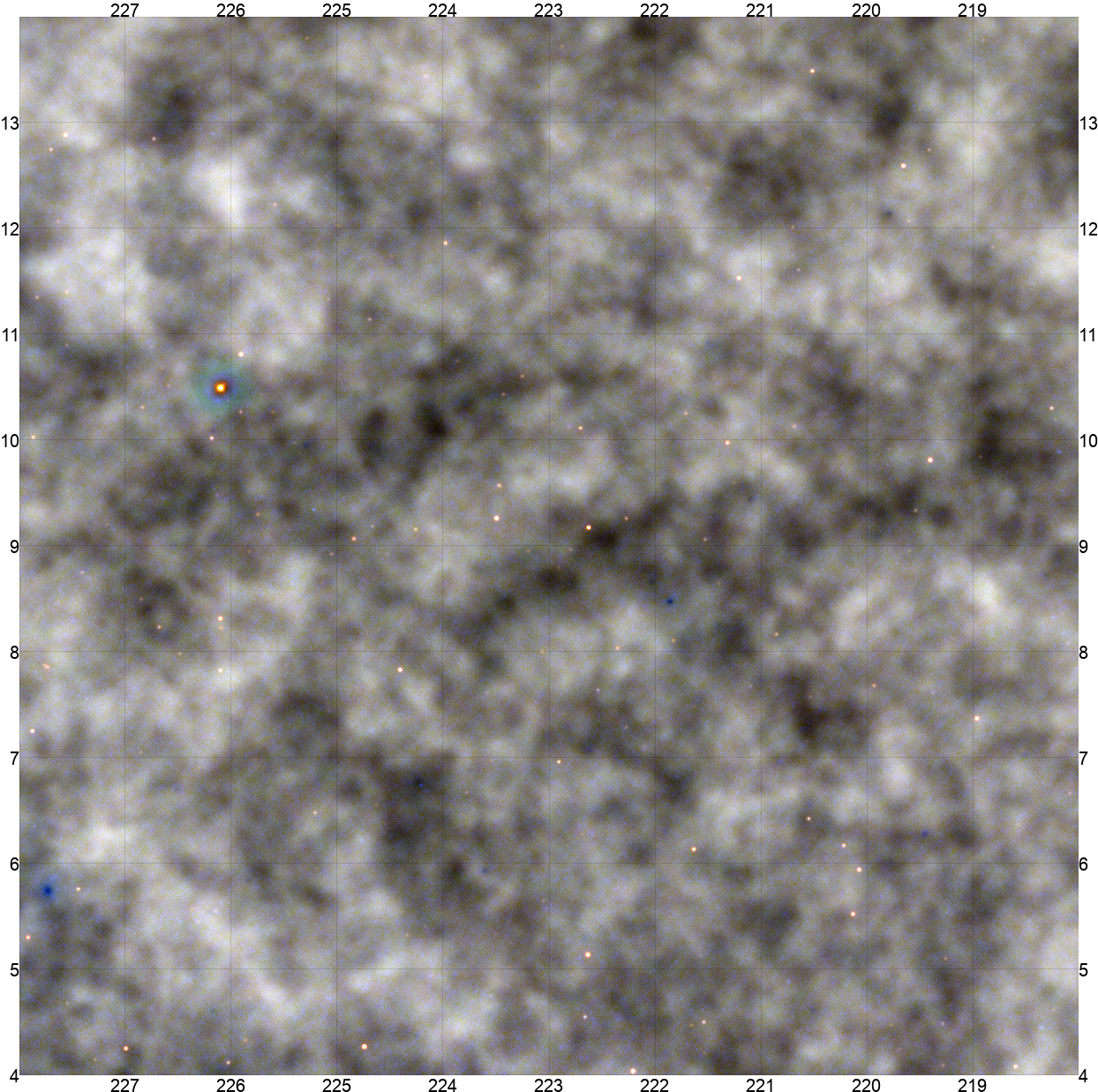
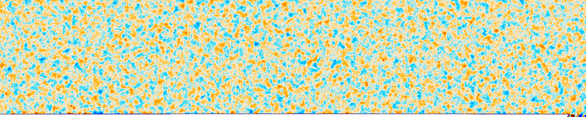
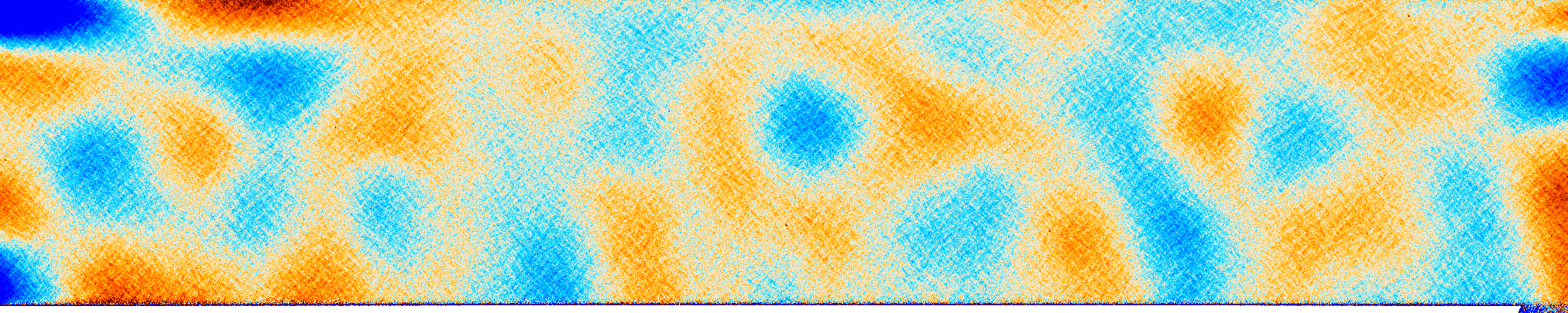
Figure 8 shows a multifrequency view of a 100 square degree subset of the ACT DR6 data, with the f090/f150/f220 bands mapped to the red/green/blue color channels of the image. This paints the CMB as a gray fog (due to having the same amplitude at all frequencies in these units); synchrotron-dominated active galactic nuclei have a falling spectrum and therefore show up as bright orange; the thermal Sunyaev Zel’dovich effect in galaxy clusters causes a power deficit in f090 and f150 but not in f220, and therefore shows up as dark blue spots; while a few nearby dusty galaxies are faintly visible in light blue. To avoid large-scale atmospheric noise visually dominating the image, we have coadded it with Planck for this plot, with Planck dominating on scales larger than about 1/3 of a degree.
Polarization for the same 100 square degree area can be found in figure 9, where we see signal-dominated E-modes and B-modes consistent with noise. While this is one of the deepest areas of the DR6 day+night map, with a frequency-combined white noise level of 4 K arcmin, there are signal-dominated E-modes over the entire 19 000 square degree DR6 area.
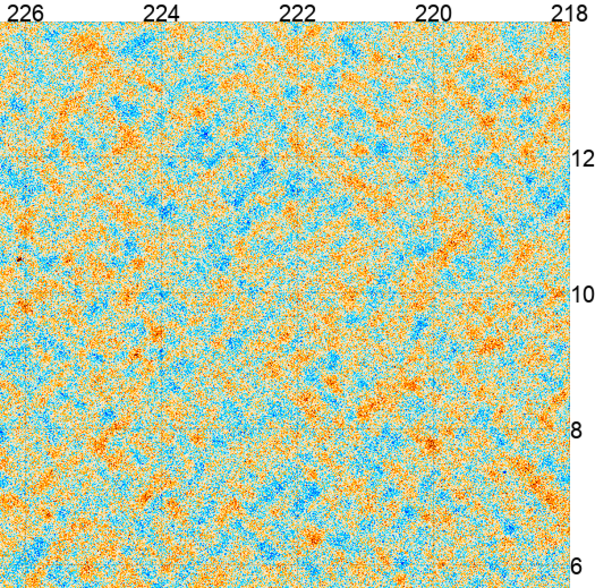
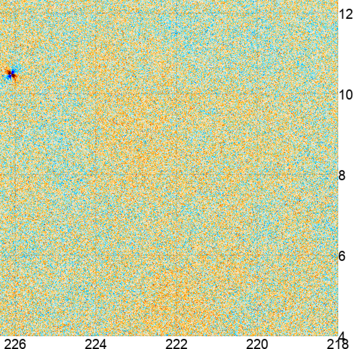
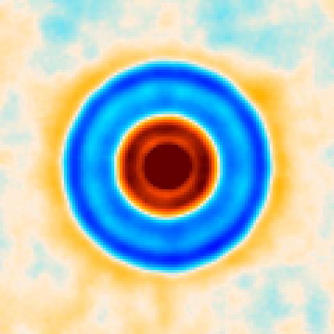
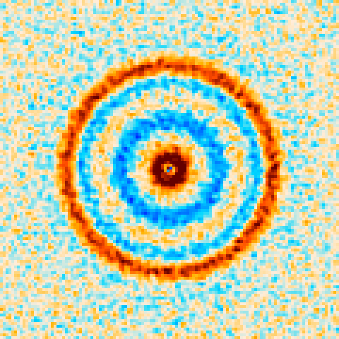
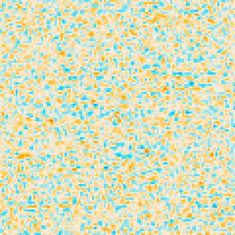
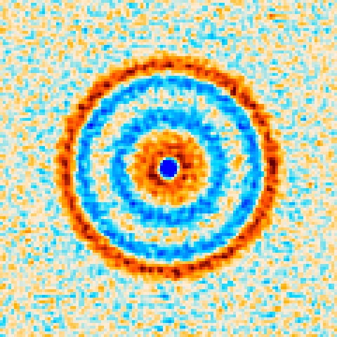
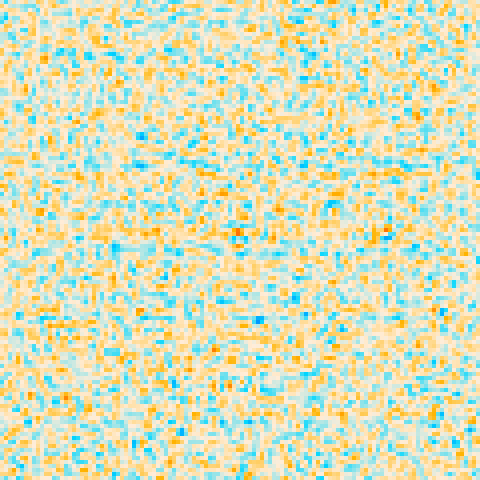
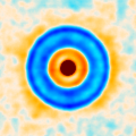
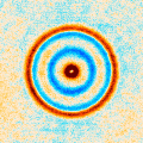
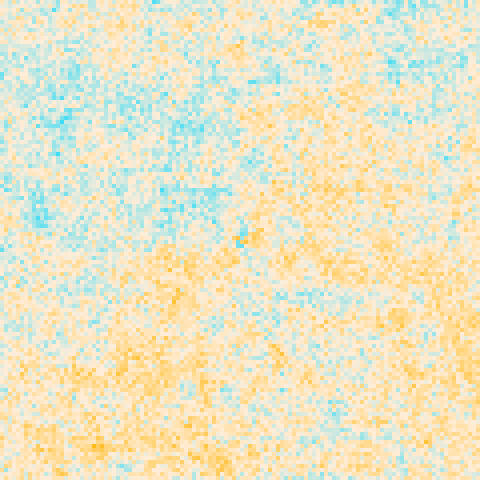
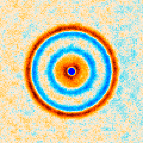
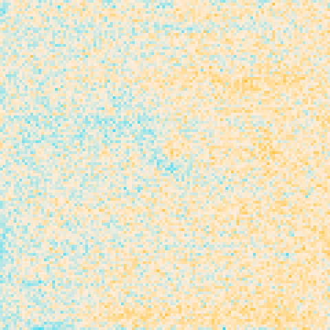
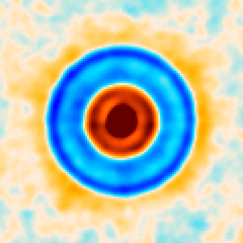
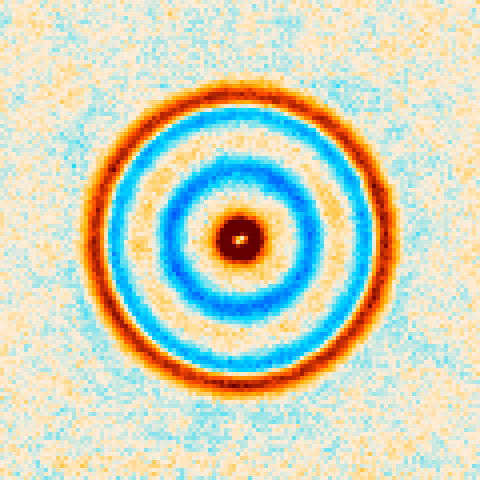
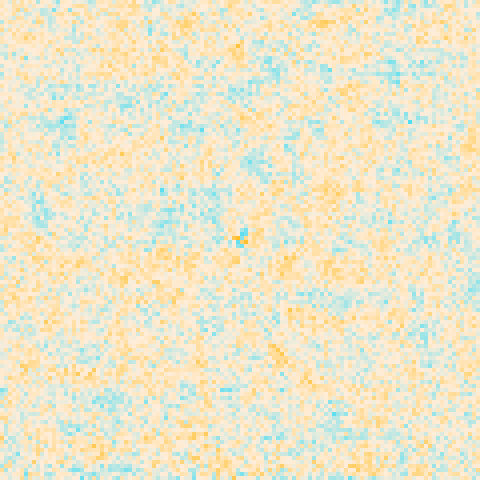
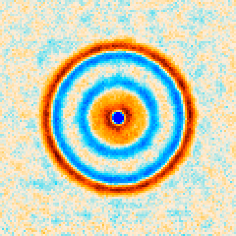
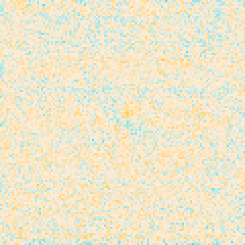
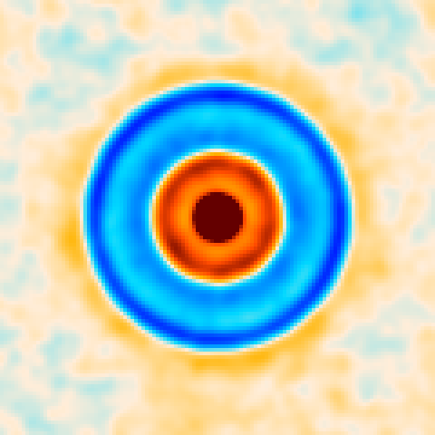
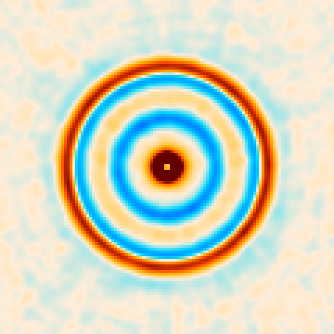
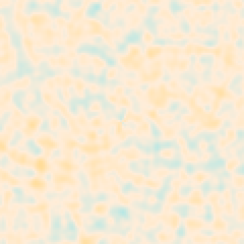
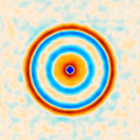
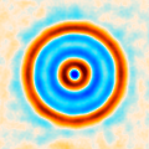
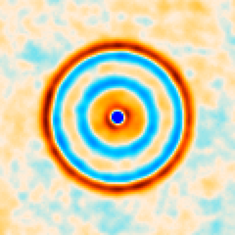
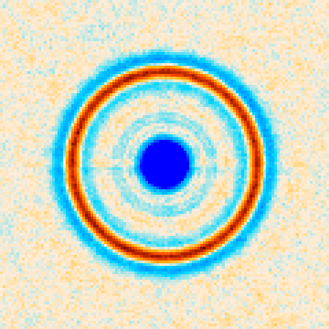
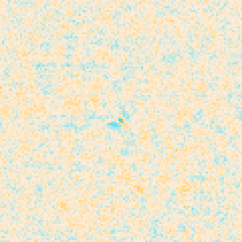
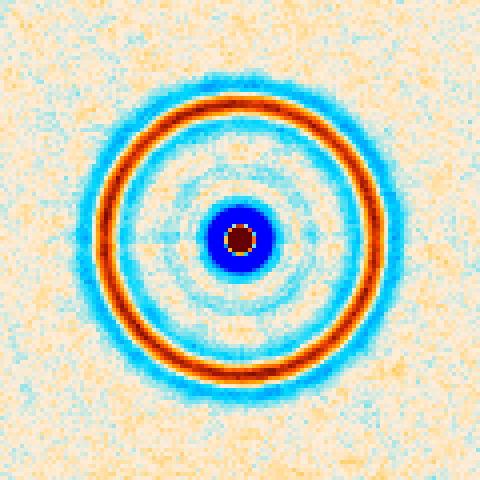
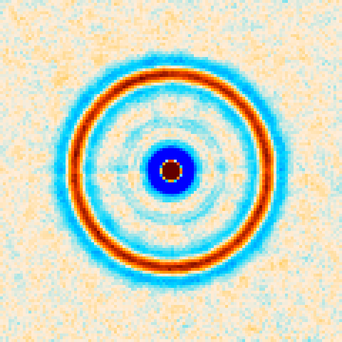
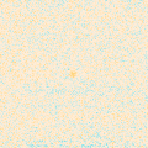
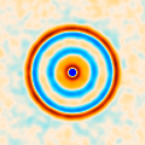
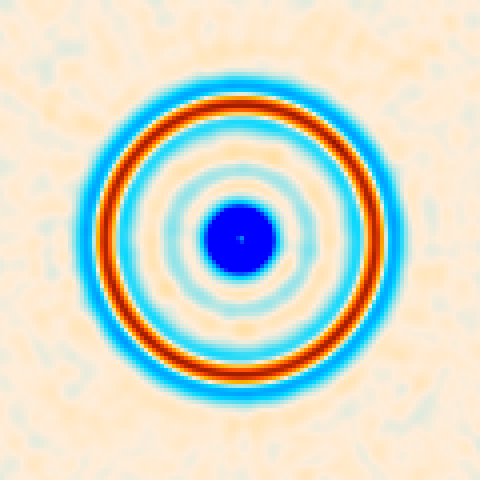
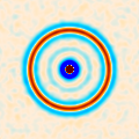
Figures 10 and 11 stack our maps on peaks in T and E respectively, as first done for WMAP in Komatsu et al. (2011), and compare them with Planck and simulations. The baryon-acoustic feature stands out with high signal-to-noise, giving a striking illustration of the causal structure at the surface of last scattering.
Finally, figure 12 overplots polarization vectors on total intensity to illustrate the correlation between the two, while figure 13 filters total intensity to highlight point sources, revealing point sources and clusters at in this 100 square degree area of the sky. Over the full ACT area, we detect 30 000 point sources and 6 000 clusters at (1.9 per square degree and 0.40 per square degree over 16 000 square degrees after masking).
T map
Time map
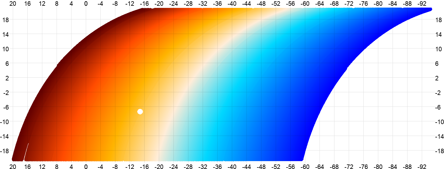
Figure 14 is a low-resolution plot of a typical depth-1 map. No CMB is visible in these shallow maps, but bright point sources and parts of the Milky Way are still visible. The time at which each pixel was hit is also shown.
5 Technical issues
5.1 Correlated noise
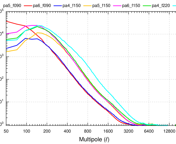
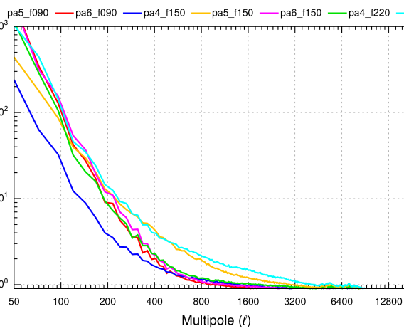
Unlike space-based CMB telescopes like Planck and WMAP, ground-based CMB telescopes have to look through the atmosphere. At these frequencies the atmosphere is only partially transparent due to spectral lines from water vapor and oxygen. Water vapor is present and clumpily distributed even when no visible clouds are present. Emission from this inhomogeneous water vapor, and to a lesser extent temperature variations in the atmosphere, are the dominant noise sources on large scales in ACT, and are responsible for the several orders of magnitude increase in noise power at low in figure 15.
| TT |
 |
| EE |
 |
The atmospheric noise can be approximated as a power law both in time domain and map space, with a slope of in both cases.222222 The intrinsic power spectrum of atmospheric turbulence has a slope of -8/3. This is steepened at small scales by near-field effects, and further modified when projected onto the sky with the telescope’s scanning pattern. The result is a spectrum with a more complicated shape that can still be approximately described as a power law with an exponent of around -3. The total map noise power spectrum is then roughly a sum of this power law and a white noise floor:
| (12) |
is the multipole where the white noise and correlated noise have equal power. As we move down from this (to larger scales) the atmospheric noise grows rapidly, and by the atmospheric noise power is times higher than the white noise. In our total intensity maps, is mainly a function of bandpass, being around 2100/3000/3800 at f090/f150/f220. In polarization the situation is more complicated, depending both on the individual array and the declination in the map. See appendix F for details. Typical numbers here are 300/450/600/500/450/640 for PA5 f090/PA6 f090/PA4 f150/PA5 f150/PA6 f150/PA4 f220.
These numbers are similar to those found in our earlier data releases and by other ground-based CMB telescopes232323SPT has at f090/f150/f220 for T and 200 for E, but a slope closer to -4 (Dibert et al., 2022). The SPT site typically has 1/3 the PWV of the ACT site., but are much higher than for space telescopes. For example, Planck has and a slope closer to . This means that while it’s a decent approximation to treat the Planck noise as white, there are hardly any cases where this is a good approximation for our maps!
5.2 Transfer function
The maximum-likelihood mapmaking estimator for an instrument that observes some sky with response is . This estimator is unbiased as long as one hasn’t done any filtering of the data beyond what is captured in the weighting matrix . If describes the covariance of the noise, then the solution is additionally optimal. When inversion of must be done using iterative methods like CG, as is the case for us, then stopping the iteration early will introduce some bias even when the data is unfiltered.
For DR6 our goal was to recover as low as possible, so unlike DR4 we chose to forego all filtering of to minimize mapmaker bias.242424 Experience from DR4 had already taught us that ground pickup could be effectively subtracted in map-space. We expected that this would leave conjugate gradient convergence as the only relevant source of bias in the mapmaking, and we confirmed this using end-to-end simulations where we estimated the mapmaker transfer function as
| (13) |
Here sim is a simulated sky map, is the same response matrix as used in the mapmaking, represents the full multi-pass mapmaking process, is the cross-spectrum of two maps, and is the power spectrum of a single map. The data needs to enter into this expression since the mapmaker needs it to build the noise model, but to first order the data cancels when the data-only map is subtracted.
The result of these end-to-end simulations is shown in figure 16. As expected this showed that our mapmaker output converged towards an unbiased result, with the number of conjugate gradient iterations being the only relevant source of bias. We also confirmed that this convergence continues beyond the 900 CG steps shown in the figure.
We were therefore surprised when we saw that our actual data converged towards a result that deviated strongly from Planck at low in total intensity, as seen in the black curve in figure 16. This was especially so since the bias took the form of a lack of power, which cannot be explained with additive systematics like ground pickup. It seemed baffling that the mapmaker should be able to treat our injected signal differently from the real data when all we were giving it was a sum of the two!
Of course, we knew that the simulations differed from the data in one small way: the beam-convolved sky we observe is smooth, but the simulation was piecewise constant inside each pixel due to the nearest-neighbor approximation used in . We had already seen that this could produce artifacts in high-contrast areas like those near bright point sources (Næss, 2019), but surely these sub-pixel details would only matter on the smallest scales in the map? But no, what we saw when we repeated the simulations with smoother, high-resolution inputs252525We simulated a map at two times the target resolution and used a bilinear pointing matrix to read it off. We also tested even higher resolution input maps. These differed slightly in the effective pixel window at high , but were robust at low . The high- behavior is well described by the ratio of the input to output pixel windows. E.g. a 0.25′ resolution bilinear simulation mapped with a 0.5′ nearest neighbor pointing matrix would result in a total pixel window of . When taking this into account, the measured transfer function was robust to the simulation resolution over all multipoles. We therefore stuck with two times the target resolution for these simulations. was that tiny sub-pixel effects could indeed cause a large loss of power at low in the mapmaker. This is shown in the magenta curve in figure 17. With the noise weighting () used for PA6 f150, nearest neighbor mapmaking with a pixel size of 0.5 arcminutes results in a 0.2%/1%/5%/25% loss of T amplitude (twice that in power) by . The effect is qualitatively similar for the other arrays, but it scales with .
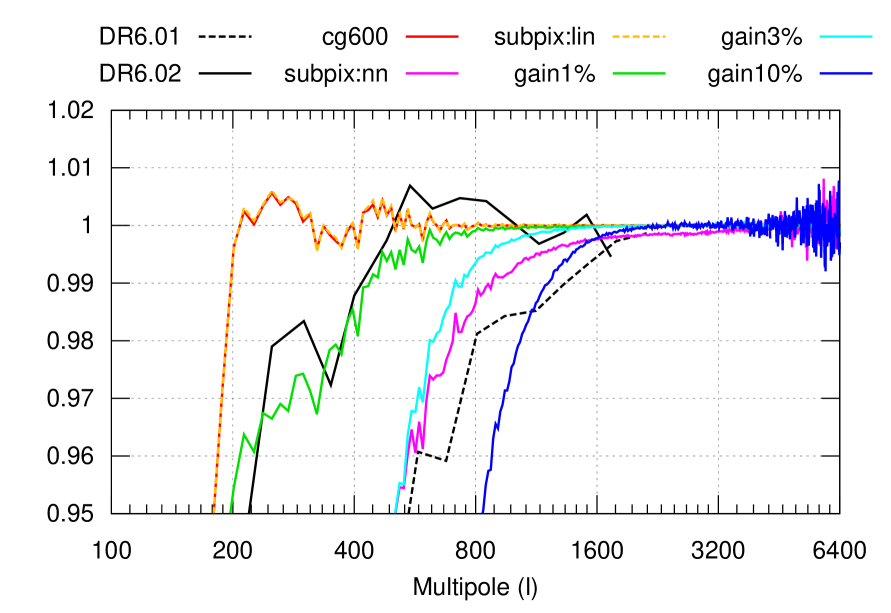
Naess & Louis (2023) analyse and describe this effect in detail, but in summary this is a manifestation of the regression dilution bias that occurs in a linear least-squares estimator when both the independent and dependent variables are noisy, not just the dependent ones. In our case, the response matrix used in the analysis is perturbed away from the true response, . This leads to a net-positive term in the denominator.
| (14) |
Here we have omitted terms that average down as more data are added, unlike the squared terms. When expressed in harmonic space, and are nearly diagonal, and so can be approximated as functions of . The inherits the slope of , but non-obviously the tiny is much shallower.262626It is practically constant for gain errors, while its slope is around half that of for nearest neighbor subpixel errors. As one goes to lower , there eventually comes a point where becomes small enough that is no longer negligible in comparison. At this point the denominator of equation 14 becomes larger than its numerator, and the amplitude of starts attenuating. This is the cause of the loss of power at low . See appendix G for more details.
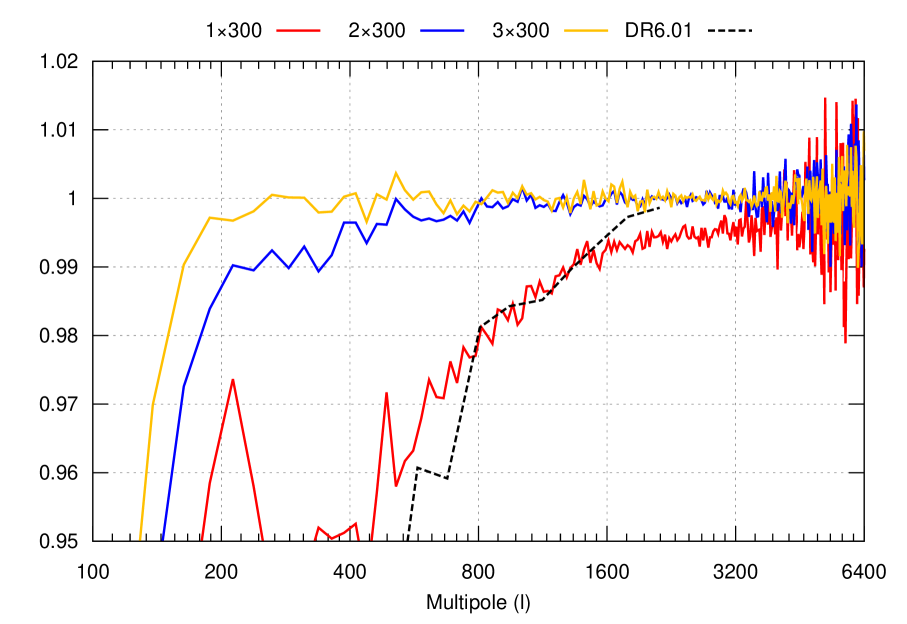
Satisfied that we had found the cause, we modified the mapmaker to use a bilinear response matrix as described in section 3.3.2, but to our disappointment part of the power loss still remained. Further investigation pointed to a relative gain miscalibration between detectors in the array as the likely culprit.272727We also investigated time constant and polarization angle errors, but these did not have an appreciable effect for reasonable error sizes. The green, light blue and dark blue curves in figure 17 show the simulated transfer function for 1%, 3% and 10% standard deviation per-detector gain errors.282828 When simulating this it is essential that the same gain errors are present both when building the noise matrix and when solving for the map, otherwise the effect will be missed! For PA6 f150 these lead to a 1% loss of signal at . This motivated the gain calibration changes in section 2.4.1.292929 This consisted of reverting to the atmospheric flatfielding we used in DR4, plus some work improving these. After these changes, the measured transfer function improved from the dashed black curve in figure 17 to the solid one, with the point of 1% signal loss moving from to 400 for PA6 f150.
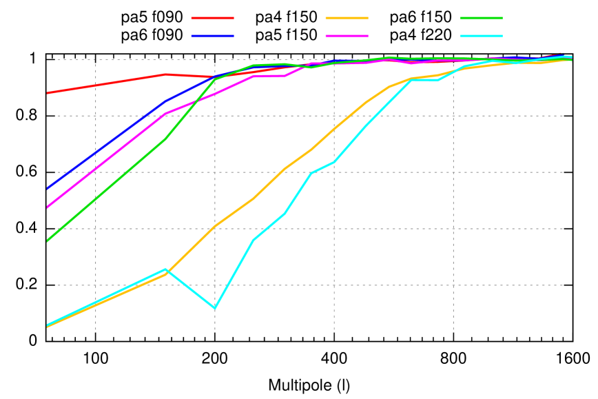
The final transfer functions after these improvements are shown in figure 18 for all the arrays in this data release. A more detailed estimate with uncertainties is reported in Louis et al. (2025). There is still considerable room for improvement: the transfer functions now reach a 1% signal loss at , except for PA4 where it happens around . We believe this is still mainly driven by gain miscalibration, but the lack of a good calibrator makes it difficult to improve further.303030 We expect that the Simons Observatory Large Aperture Telescope, which in many respects is ACT’s successor, will be much less impacted by this effect due to the gain calibrator built into its primary mirror. In principle, one could solve jointly for both the sky and the per-detector, per-TOD313131Or some other suitable timescale over which the gain are hopefully stable. gains. We have demonstrated that this works in small toy examples, but convergence is hopelessly slow for realistic data sets. Solving this efficiently is an open problem in CMB mapmaking, but perhaps of low importance since low- total intensity has already been exquisitely measured by Planck and WMAP.
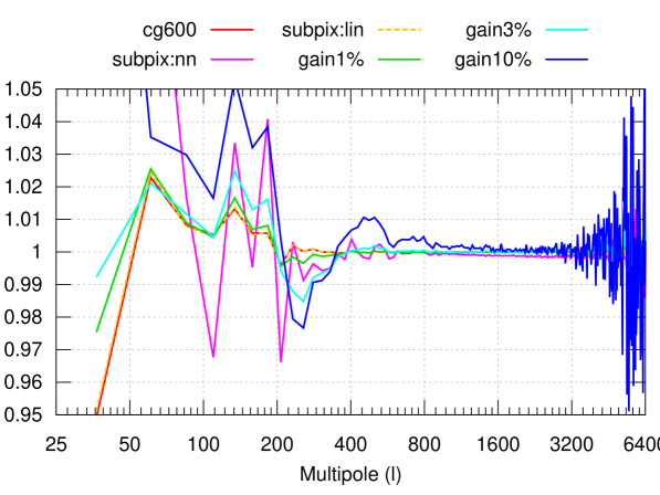
As we saw in section 5.1, the polarized is as high as in total intensity. The from equation 14 will therefore reach levels where is relevant at times as high multipole, so a priori we would expect the polarized transfer function to deviate less than 1% from unity for . Figure 19 shows the polarized transfer function from simulations. Unlike total intensity there are no clear trends, but the larger scatter makes it hard to quantify the behavior for . For the 1% gain error case that best matches our T transfer function, the polarization transfer function deviation from 1 is less than 0.005% for and less than 0.2% for . The scatter could be reduced with more simulations, but since we do not consider in our cosmological likelihood, this is sufficient for DR6.
5.3 Pickup contamination
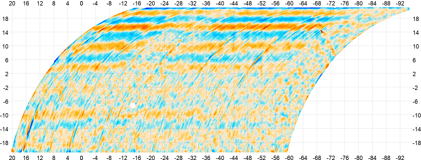
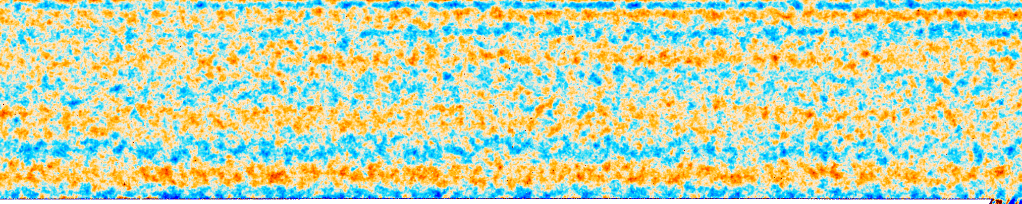
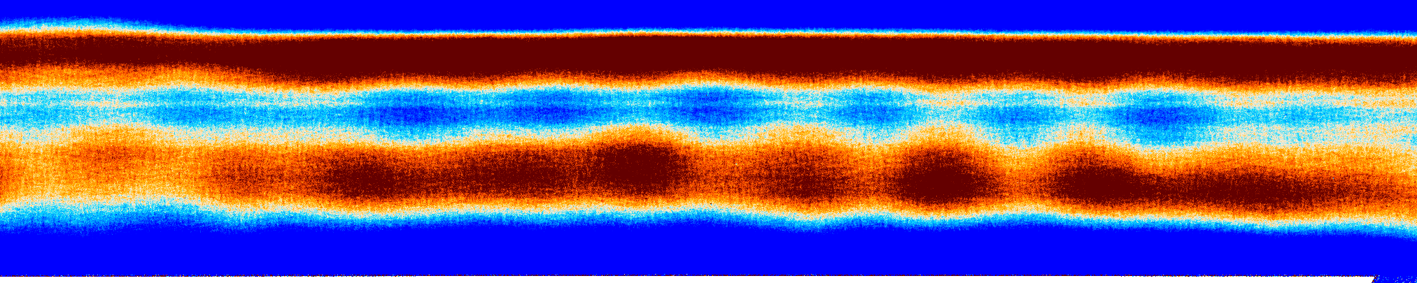
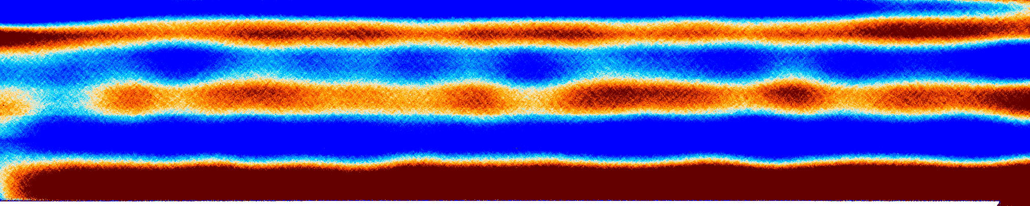
An example of a raw DR6 map is shown at the top of figure 20. It is visibly dominated by bright horizontal bands of azimuth-synchronous pickup in polarization, with an amplitude of µK. These bands are less visible in total intensity, but have roughly the same amplitude there. Some of this is caused by sidelobes hitting corners of the ground screen, but much of it appears to be pickup of uncertain origin internal to the telescope.
Raw map
T
 Q
Q
 U
U
After removing
T
 Q
Q
 U
U
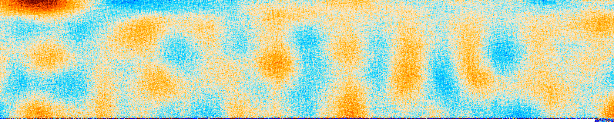
Despite their dire appearance, these stripes do not impact the maps’ usefulness much due to occupying a tiny region of harmonic space. We find that a very gentle filter that simply removes spherical harmonics modes with , or equivalently in 2D Fourier space, is enough to make the maps visually pickup free (see bottom of figure 20). For our power spectrum analysis, however, we found that a stricter cut of () was necessary to pass our null tests.323232The discrepancy beteen and arises because we use the average pixel size in the map to calculate . 2D Fourier space is based on the flat-sky approximation, so the correspondence between Fourier wavenumbers and is always approximate. For our patch, .,333333The power spectrum analysis also removes , but this is motivated by correlated noise, not pickup. We interpret this as residual pickup too faint to make out by eye. See also section 3.3.1 of Louis et al. (2025).
It is because of this relatively simple structure of the pickup in the maps that we chose to forego time-domain pickup subtraction in section 3.1. The bias introduced by subtraction there would have been much more expensive to characterize, requiring full time-domain simulations, while not necessarily being as effective as the map-level simulation at removing all the pickup. For example, in DR4 we found that TOD-level filtering did not clean the data sufficiently, requiring map-level filtering anyway, in the form of the “k-space filter”.
6 Conclusion
We have presented the ACT DR6 maps, based on the 2017–2022 survey with the AdvancedACT camera. The maps, which cover the three frequency bands f090, f150 and f220 with an angular resolution of 1.4′ at f150, fall into two categories: Average sky maps, which cover 45% of the sky with a median frequency-combined depth of 10 µK′; and more than ten thousand single-scan “depth-1 maps” with a typical depth of 250 µK ( mJy) that are suitable for time domain astronomy.
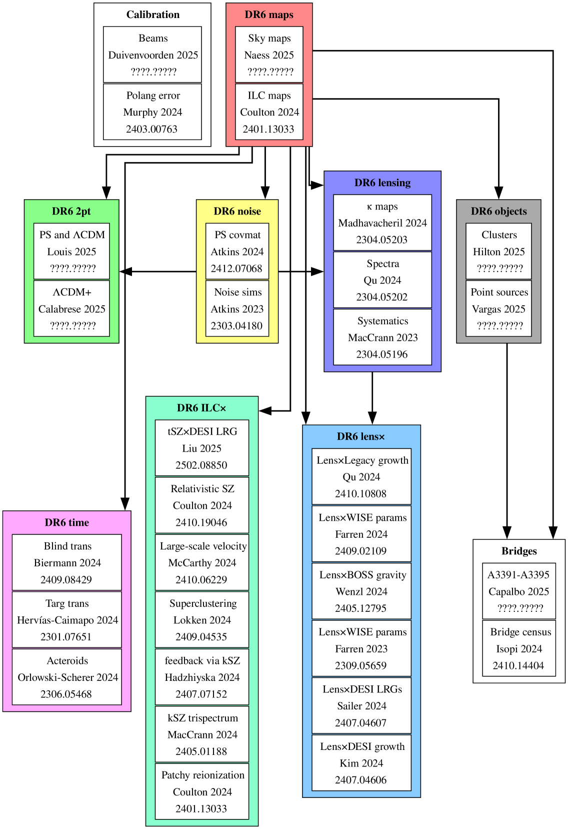
These maps form the basis of the rest of the DR6 analysis effort, as laid out in figure 21. The DR6.02 maps’ angular power spectra and fit to CDM are described in Louis et al. (2025), and extensions to CDM are evaluated in Calabrese et al. (2025). Vargas et al. (2025) and Hilton et al. (2025) use the maps to detect around 30,000 point sources at and find optically confirmed galaxy clusters ( at ). DR6.01 maps were used to produce weak lensing maps (Madhavacheril et al., 2024) and power spectra (Qu et al., 2024), as well as component-separated maps (Coulton et al., 2024). These in turn were used in a large number of cross-correlation studies. The depth-1 maps are used to in blind (Biermann et al., 2024) and targeted (Herv´ıas-Caimapo et al., 2024) transient searches, and Orlowski-Scherer et al. (2024) uses them to study solar system asteroids.
We make the maps available on the Legacy Archive for Microwave Background Data Analysis (LAMBDA) at https://lambda.gsfc.nasa.gov/product/act/actadv_prod_table.html and at NERSC at /global/cfs/cdirs/cmb/data/act_dr6/dr6.02. With the exception of the depth-1 maps and the null test maps, the maps are also made available reprojected to HEALPix. An interactive web atlas is available at https://phy-act1.princeton.edu/public/snaess/actpol/dr6/atlas/. Some of the coadd maps are also published in the Aladin interactive sky atlas (Bonnarel et al., 2000), e.g. https://alasky.cds.unistra.fr/ACT/DR4DR6/color_CMB.
While the DR6 maps cover most of the AdvancedACT data, there is still substantial unexploited potential. The PA7 low-frequency array was installed in 2020 and covered two new frequency bands, f030 and f040. We hope to publish these maps in a future DR7. Also, as discussed in sections 5.1 and 5.2, gain calibration issues are implicated in the low- power loss in total intensity and correlated noise excess in low- polarization. A future analysis may be able to substantially improve on this. Beyond ACT, the Simons Observatory Large Aperture Telescope is expected to begin observations soon. It will cover a superset of the DR6 sky area in six frequency bands at a combined depth of µK′.
Acknowledgements
Resources
Support for ACT was through the U.S. National Science Foundation through awards AST-0408698, AST-0965625, and AST-1440226 for the ACT project, as well as awards PHY-0355328, PHY-0855887 and PHY-1214379. Funding was also provided by Princeton University, the University of Pennsylvania, and a Canada Foundation for Innovation (CFI) award to UBC. ACT operated in the Parque Astronómico Atacama in northern Chile under the auspices of the Agencia Nacional de Investigación y Desarrollo (ANID). The development of multichroic detectors and lenses was supported by NASA grants NNX13AE56G and NNX14AB58G. Detector research at NIST was supported by the NIST Innovations in Measurement Science program. Computing for ACT was performed using the Princeton Research Computing resources at Princeton University and the Niagara supercomputer at the SciNet HPC Consortium. SciNet is funded by the CFI under the auspices of Compute Canada, the Government of Ontario, the Ontario Research Fund–Research Excellence, and the University of Toronto. This research also used resources of the National Energy Research Scientific Computing Center (NERSC), a U.S. Department of Energy Office of Science User Facility located at Lawrence Berkeley National Laboratory, operated under Contract No. DE-AC02-05CH11231 using NERSC award HEP-ERCAPmp107 from 2021 to 2025. We thank the Republic of Chile for hosting ACT in the northern Atacama, and the local indigenous Licanantay communities whom we follow in observing and learning from the night sky.
We are grateful to the NASA LAMBDA archive for hosting our data. This work uses data from the Planck satellite, based on observations obtained with Planck (http://www.esa.int/Planck), an ESA science mission with instruments and contributions directly funded by ESA Member States, NASA, and Canada.
SN, MH, SA and DNS acknowledge support from Simons Foundation. This work was supported by a grant from the Simons Foundation (CCA 918271, PBL). IA acknowledges support from Fundación Mauricio y Carlota Botton and the Cambridge International Trust. ZA and JD acknowledge support from NSF grant AST-2108126. EC, IH and HTJ acknowledge support from the Horizon 2020 ERC Starting Grant (Grant agreement No 849169). JD acknowledges support from a Royal Society Wolfson Visiting Fellowship and from the Kavli Institute for Cosmology Cambridge and the Institute of Astronomy, Cambridge. RD thanks ANID for grants BASAL CATA FB210003, FONDEF ID21I10236 and QUIMAL240004. SG acknowledges support from STFC and UKRI (grant numbers ST/W002892/1 and ST/X006360/1). VG acknowledges the support from NASA through the Astrophysics Theory Program, Award Number 21-ATP21-0135, the National Science Foundation (NSF) CAREER Grant No. PHY2239205, and from the Research Corporation for Science Advancement under the Cottrell Scholar Program. This research was carried out in part at the Jet Propulsion Laboratory, California Institute of Technology, under a contract with the National Aeronautics and Space Administration (80NM0018D0004). JCH acknowledges support from NSF grant AST-2108536, the Sloan Foundation, and the Simons Foundation, and thanks the Scientific Computing Core staff at the Flatiron Institute for computational support. MH acknowledges support from the National Research Foundation of South Africa (grant no. 137975). ADH acknowledges support from the Sutton Family Chair in Science, Christianity and Cultures, from the Faculty of Arts and Science, University of Toronto, and from the Natural Sciences and Engineering Research Council of Canada (NSERC) [RGPIN-2023-05014, DGECR-2023-00180]. JPH (George A. and Margaret M. Downsbrough Professor of Astrophysics) acknowledges the Downsbrough heirs and the estate of George Atha Downsbrough for their support. JK, MSM and KPS acknowledge support from NSF grants AST-2307727 and AST-2153201. ALP acknowledges support from a Science and Technology Facilities Council (STFC) Consolidated Grant (ST/W000903/1). ML acknowledges that IFAE is partially funded by the CERCA program of the Generalitat de Catalunya. TN thanks support from JSPS KAKENHI Grant No. JP20H05859, No. JP22K03682, and World Premier International Research Center Initiative (WPI Initiative), MEXT, Japan. FN acknowledges funding from the European Union (ERC, POLOCALC, 101096035). LAP acknowledges support from the Wilkinson and Misrahi Funds. KKR is supported by an Ernest Rutherford Fellowship from the UKRI Science and Technology Facilities Council (grant number ST/Z510191/1). NS acknowledges support from DOE award number DE-SC0025309. CS acknowledges support from the Agencia Nacional de Investigación y Desarrollo (ANID) through Basal project FB210003. KS acknowledges support from the NSF Graduate Research Fellowship Program under Grant No. DGE 2036197, and acknowledges the use of computing resources from Columbia University’s Shared Research Computing Facility project, which is supported by NIH Research Facility Improvement Grant 1G20RR030893-01, and associated funds from the New York State Empire State Development, Division of Science Technology and Innovation (NYSTAR) Contract C090171, both awarded April 15, 2010.
Software
We gratefully acknowledge the many publicly available software packages that were essential for parts of this analysis. They include healpy (Zonca et al., 2019), HEALPix (Górski et al., 2005), DUCC (Reinecke, 2020) and pixell343434https://github.com/simonsobs/pixell. This research made use of Astropy353535http://www.astropy.org, a community-developed core Python package for Astronomy (Astropy Collaboration, 2013; Price-Whelan et al., 2018). We also acknowledge use of the matplotlib (Hunter, 2007) package and the Python Image Library for producing plots in this paper.
References
- 4MOST (2024) 4MOST. 2024, Survey simulations, , https://www.4most.eu/cms/operations/surveysimulations
- Abbott et al. (2021) Abbott, T. M. C., et al. 2021, arXiv:2101.05765, ApJS, 255, 20, The Dark Energy Survey Data Release 2
- Adachi et al. (2022) Adachi, S., et al. 2022, arXiv:2203.02495, ApJ, 931, 101, Improved Upper Limit on Degree-scale CMB B-mode Polarization Power from the 670 Square-degree POLARBEAR Survey
- Ade et al. (2022a) Ade, P. A. R., et al. 2022a, arXiv:2103.13334, ApJ, 927, 174, A Constraint on Primordial B-modes from the First Flight of the SPIDER Balloon-borne Telescope
- Ade et al. (2022b) —. 2022b, arXiv:2110.00482, ApJ, 927, 77, BICEP/Keck XV: The BICEP3 Cosmic Microwave Background Polarimeter and the First Three-year Data Set
- Ahumada et al. (2020) Ahumada, R., et al. 2020, arXiv:1912.02905, ApJS, 249, 3, The 16th Data Release of the Sloan Digital Sky Surveys: First Release from the APOGEE-2 Southern Survey and Full Release of eBOSS Spectra
- Aiola et al. (2020) Aiola, S., et al. 2020, arXiv:2007.07288, J. Cosmology Astropart. Phys, 2020, 047, The Atacama Cosmology Telescope: DR4 maps and cosmological parameters
- ALMA (2019) ALMA. 2019, ALMA calibrator catalogue, https://almascience.eso.org/alma-data/calibrator-catalogue, accessed: 2019-12-07
- Astropy Collaboration (2013) Astropy Collaboration. 2013, arXiv:1307.6212, A&A, 558, A33, Astropy: A community Python package for astronomy
- Atkins et al. (2023) Atkins, Z., et al. 2023, arXiv:2303.04180, J. Cosmology Astropart. Phys, 2023, 073, The Atacama Cosmology Telescope: map-based noise simulations for DR6
- Balkenhol et al. (2023) Balkenhol, L., et al. 2023, arXiv:2212.05642, Phys. Rev. D, 108, 023510, Measurement of the CMB temperature power spectrum and constraints on cosmology from the SPT-3G 2018 T T , T E , and E E dataset
- Benson et al. (2014) Benson, B. A., et al. 2014, arXiv:1407.2973, 9153, 91531P, SPT-3G: a next-generation cosmic microwave background polarization experiment on the South Pole telescope
- BICEP2/Keck Collaboration (2018) BICEP2/Keck Collaboration. 2018, arXiv:1810.05216, Phys. Rev. Lett., 121, 221301, Constraints on Primordial Gravitational Waves Using Planck, WMAP, and New BICEP2/Keck Observations through the 2015 Season
- Biermann et al. (2024) Biermann, E. K., et al. 2024, arXiv:2409.08429, arXiv e-prints, arXiv:2409.08429, The Atacama Cosmology Telescope: Systematic Transient Search of Single Observation Maps
- Bonnarel et al. (2000) Bonnarel, F., et al. 2000, A&AS, 143, 33, The ALADIN interactive sky atlas. A reference tool for identification of astronomical sources
- Calabrese et al. (2025) Calabrese, E. et al. 2025, in preparation, The Atacama Cosmology Telescope: DR6 beyond LCDM parameters
- Choi et al. (2018) Choi, S. K., et al. 2018, arXiv:1711.04841, JLTP, 193, 267, Characterization of the Mid-Frequency Arrays for Advanced ACTPol
- Choi et al. (2020) —. 2020, arXiv:2007.07289, J. Cosmology Astropart. Phys, 2020, 045, The Atacama Cosmology Telescope: a measurement of the Cosmic Microwave Background power spectra at 98 and 150 GHz
- Condon et al. (1998) Condon, J. J., Cotton, W. D., Greisen, E. W., Yin, Q. F., Perley, R. A., Taylor, G. B., & Broderick, J. J. 1998, AJ, 115, 1693, The NRAO VLA Sky Survey
- Coulton et al. (2024) Coulton, W. R., et al. 2024, arXiv:2401.13033, arXiv e-prints, arXiv:2401.13033, The Atacama Cosmology Telescope: Detection of Patchy Screening of the Cosmic Microwave Background
- Crowley et al. (2018) Crowley, K. T., et al. 2018, arXiv:1807.07496, Journal of Low Temperature Physics, 193, 328, Advanced ACTPol TES Device Parameters and Noise Performance in Fielded Arrays
- Cutri et al. (2021) Cutri, R. M., et al. 2021, VizieR Online Data Catalog, II/328, VizieR Online Data Catalog: AllWISE Data Release (Cutri+ 2013)
- Dibert et al. (2022) Dibert, K. R., et al. 2022, arXiv:2205.04494, Phys. Rev. D, 106, 063502, Forecasting ground-based sensitivity to the Rayleigh scattering of the CMB in the presence of astrophysical foregrounds
- Duivenvoorden et al. (in prep) Duivenvoorden, A. et al. in prep, The Atacama Cosmology Telescope: beam measurements for DR6
- Dünner et al. (2013) Dünner, R., et al. 2013, arXiv:1208.0050, ApJ, 762, 10, The Atacama Cosmology Telescope: Data Characterization and Mapmaking
- Euclid Collaboration et al. (2022) Euclid Collaboration, et al. 2022, arXiv:2108.01201, A&A, 662, A112, Euclid preparation. I. The Euclid Wide Survey
- Fowler (2014) Fowler, J. 2014, Slim: Numerical data compression for scientific data sets, Astrophysics Source Code Library, record ascl:1409.010
- Ge et al. (2024) Ge, F., et al. 2024, arXiv:2411.06000, arXiv e-prints, arXiv:2411.06000, Cosmology From CMB Lensing and Delensed EE Power Spectra Using 2019-2020 SPT-3G Polarization Data
- Górski et al. (2005) Górski, K. M., Hivon, E., Banday, A. J., Wandelt, B. D., Hansen, F. K., Reinecke, M., & Bartelmann, M. 2005, arXiv:astro-ph/0409513, ApJ, 622, 759, HEALPix: A Framework for High-Resolution Discretization and Fast Analysis of Data Distributed on the Sphere
- Gualtieri et al. (2018) Gualtieri, R., et al. 2018, arXiv:1711.10596, Journal of Low Temperature Physics, 193, 1112, SPIDER: CMB Polarimetry from the Edge of Space
- Guidi (2022) Guidi, F. 2022, Cosmology from SPT-3G, https://agenda.infn.it/event/28896/contributions/164821/attachments/91724/124648/11%20-%20Guidi_CMBFerrara.pdf
- Hahn et al. (2023) Hahn, C., et al. 2023, arXiv:2208.08512, AJ, 165, 253, The DESI Bright Galaxy Survey: Final Target Selection, Design, and Validation
- Hasselfield et al. (2013) Hasselfield, M., et al. 2013, arXiv:1303.4714, ApJS, 209, 17, The Atacama Cosmology Telescope: Beam Measurements and the Microwave Brightness Temperatures of Uranus and Saturn
- Henderson et al. (2016) Henderson, S. W., et al. 2016, arXiv:1607.06064, in Proc. SPIE, Vol. 9914, Society of Photo-Optical Instrumentation Engineers (SPIE) Conference Series, 99141G
- Herv´ıas-Caimapo et al. (2024) Hervías-Caimapo, C., et al. 2024, arXiv:2301.07651, MNRAS, 529, 3020, The Atacama cosmology telescope: flux upper limits from a targeted search for extragalactic transients
- Hilton et al. (2025) Hilton, M. et al. 2025, in preparation, The Atacama Cosmology Telescope: DR6 tSZ-detected galaxy clusters
- Hinshaw et al. (2013) Hinshaw, G., et al. 2013, AJS, 208, 19, Nine-Year Wilkinson Microwave Anisotropy Probe (WMAP) observations: cosmological parameter results, http://dx.doi.org/10.1088/0067-0049/208/2/19
- Hoffleit & Warren (1995) Hoffleit, D. & Warren, W. H., J. 1995, VizieR Online Data Catalog, V/50, VizieR Online Data Catalog: Bright Star Catalogue, 5th Revised Ed. (Hoffleit+, 1991)
- HSC (2021) HSC. 2021, Final Survey Footprint, https://hsc.mtk.nao.ac.jp/ssp/survey
- Hunter (2007) Hunter, J. D. 2007, Computing in Science & Engineering, 9, 90, Matplotlib: A 2D graphics environment
- Kamionkowski et al. (1997) Kamionkowski, M., Kosowsky, A., & Stebbins, A. 1997, astro-ph/9611125, Phys. Rev. D, 55, 7368, Statistics of cosmic microwave background polarization
- Komatsu et al. (2011) Komatsu, E., et al. 2011, arXiv:1001.4538, ApJS, 192, 18, Seven-year Wilkinson Microwave Anisotropy Probe (WMAP) Observations: Cosmological Interpretation
- Koopman et al. (2016) Koopman, B., et al. 2016, arXiv:1607.01825, in Society of Photo-Optical Instrumentation Engineers (SPIE) Conference Series, Vol. 9914, Millimeter, Submillimeter, and Far-Infrared Detectors and Instrumentation for Astronomy VIII, ed. W. S. Holland & J. Zmuidzinas, 99142T
- Lacy et al. (2020) Lacy, M., et al. 2020, arXiv:1907.01981, PASP, 132, 035001, The Karl G. Jansky Very Large Array Sky Survey (VLASS). Science Case and Survey Design
- Li et al. (2021) Li, Y., et al. 2021, arXiv:2101.02658, IEEE Transactions on Applied Superconductivity, 31, 3063334, In Situ Performance of the Low Frequency Array for Advanced ACTPol
- Li et al. (2025) —. 2025, arXiv:2501.11904, arXiv e-prints, arXiv:2501.11904, A Measurement of the Largest-Scale CMB E-mode Polarization with CLASS
- Louis et al. (2025) Louis, T. et al. 2025, in preparation, The Atacama Cosmology Telescope: DR6 Power spectra, Likelihood and LCDM parameters
- LSST (2023) LSST. 2023, Survey Cadence Optimization Committee’s Phase 2 Recommendations, https://pstn-055.lsst.io/PSTN-055.pdf
- Lungu et al. (2022) Lungu, M., et al. 2022, arXiv:2112.12226, J. Cosmology Astropart. Phys, 2022, 044, The Atacama Cosmology Telescope: measurement and analysis of 1D beams for DR4
- Madhavacheril et al. (2024) Madhavacheril, M. S., et al. 2024, arXiv:2304.05203, ApJ, 962, 113, The Atacama Cosmology Telescope: DR6 Gravitational Lensing Map and Cosmological Parameters
- Makarov et al. (2014) Makarov, D., Prugniel, P., Terekhova, N., Courtois, H., & Vauglin, I. 2014, arXiv:1408.3476, A&A, 570, A13, HyperLEDA. III. The catalogue of extragalactic distances
- McConnell et al. (2020) McConnell, D., et al. 2020, arXiv:2012.00747, PASA, 37, e048, The Rapid ASKAP Continuum Survey I: Design and first results
- Morris et al. (2024) Morris, T. W., et al. 2024, arXiv:2410.13064, arXiv e-prints, arXiv:2410.13064, The Atacama Cosmology Telescope: Quantifying Atmospheric Emission above Cerro Toco
- Murphy et al. (2024) Murphy, C. C., et al. 2024, arXiv:2403.00763, Appl. Opt., 63, 5079, Optical modeling of systematic uncertainties in detector polarization angles for the Atacama Cosmology Telescope
- Murphy et al. (2010) Murphy, T., et al. 2010, arXiv:0911.0002, MNRAS, 402, 2403, The Australia Telescope 20 GHz Survey: the source catalogue
- Myers et al. (2003) Myers, S. T., et al. 2003, VizieR Online Data Catalog, VIII/72, VizieR Online Data Catalog: CLASS survey of radio sources (Myers+, 2003)
- Naess & Louis (2023) Naess, S. & Louis, T. 2023, arXiv:2210.02243, The Open Journal of Astrophysics, 6, 21, Large-scale power loss in ground-based CMB mapmaking
- Naess et al. (2014) Naess, S., et al. 2014, arXiv:1405.5524, J. Cosmology Astropart. Phys, 2014, 007, The Atacama Cosmology Telescope: CMB polarization at 200 < l < 9000
- Naess et al. (2020) —. 2020, arXiv:2007.07290, J. Cosmology Astropart. Phys, 2020, 046, The Atacama Cosmology Telescope: arcminute-resolution maps of 18 000 square degrees of the microwave sky from ACT 2008-2018 data combined with Planck
- Næss (2019) Næss, S. K. 2019, arXiv:1906.08030, J. Cosmology Astropart. Phys, 2019, 060, How to avoid X’es around point sources in maximum likelihood CMB maps
- Netterfield et al. (2002) Netterfield, C. B., et al. 2002, astro-ph/0104460, ApJ, 571, 604, A Measurement by BOOMERANG of Multiple Peaks in the Angular Power Spectrum of the Cosmic Microwave Background
- Norris (2011) Norris, R. P. 2011, arXiv:1111.6317, Journal of Astrophysics and Astronomy, 32, 599, Evolutionary Map of the Universe: Tracing Clusters to High Red-shift
- Orlowski-Scherer et al. (2024) Orlowski-Scherer, J., et al. 2024, arXiv:2306.05468, ApJ, 964, 138, The Atacama Cosmology Telescope: Millimeter Observations of a Population of Asteroids or: ACTeroids
- Patanchon et al. (2008) Patanchon, G., et al. 2008, arXiv:0711.3462, ApJ, 681, 708, SANEPIC: A Mapmaking Method for Time Stream Data from Large Arrays
- Planck Collaboration (2016) Planck Collaboration. 2016, arXiv:1605.08633, A&A, 596, A110, Planck intermediate results. XLIX. Parity-violation constraints from polarization data
- Planck Collaboration (2017) —. 2017, arXiv:1612.07151, A&A, 607, A122, Planck intermediate results. LII. Planet flux densities
- Planck Collaboration (2020) —. 2020, arXiv:1807.06205, A&A, 641, A1, Planck 2018 results. I. Overview and the cosmological legacy of Planck
- Price-Whelan et al. (2018) Price-Whelan, A. M., et al. 2018, AJ, 156, 123, The Astropy Project: Building an Open-science Project and Status of the v2.0 Core Package
- Qu et al. (2024) Qu, F. J., et al. 2024, arXiv:2304.05202, ApJ, 962, 112, The Atacama Cosmology Telescope: A Measurement of the DR6 CMB Lensing Power Spectrum and Its Implications for Structure Growth
- Reinecke (2020) Reinecke, M. 2020, DUCC: Distinctly Useful Code Collection, Astrophysics Source Code Library, record ascl:2008.023, https://gitlab.mpcdf.mpg.de/mtr/ducc
- Reinecke & Seljebotn (2013) Reinecke, M. & Seljebotn, D. S. 2013, arXiv:1303.4945, A&A, 554, A112, Libsharp - spherical harmonic transforms revisited
- Skrutskie et al. (2006) Skrutskie, M. F., et al. 2006, AJ, 131, 1163, The Two Micron All Sky Survey (2MASS)
- Smoot et al. (1992) Smoot, G. F., et al. 1992, ApJ, 396, L1, Structure in the COBE differential microwave radiometer first-year maps
- Souchay et al. (2015) Souchay, J., et al. 2015, A&A, 583, A75, The third release of the Large Quasar Astrometric Catalog (LQAC-3): a compilation of 321 957 objects
- Spergel et al. (2003) Spergel, D. N., et al. 2003, astro-ph/0302209, ApJS, 148, 175, First-Year Wilkinson Microwave Anisotropy Probe (WMAP) Observations: Determination of Cosmological Parameters
- Thornton et al. (2016) Thornton, R. J., et al. 2016, arXiv:1605.06569, ApJS, 227, 21, The Atacama Cosmology Telescope: The Polarization-sensitive ACTPol Instrument
- Vargas et al. (2025) Vargas, C. et al. 2025, in preparation, The Atacama Cosmology Telescope: DR6 point sources
- Waldvogel (2006) Waldvogel, J. 2006, BIT, 46, 195–202, Fast Construction of the Fejér and Clenshaw–Curtis Quadrature Rules, https://people.math.ethz.ch/˜waldvoge/Papers/fejer.html
- Weiland et al. (2011) Weiland, J. L., et al. 2011, arXiv:1001.4731, ApJS, 192, 19, Seven-year Wilkinson Microwave Anisotropy Probe (WMAP) Observations: Planets and Celestial Calibration Sources
- Wiebe et al. (2015) Wiebe, D. V., Netterfield, C. B., & Kisner, T. S. 2015, GetData: A filesystem-based, column-oriented database format for time-ordered binary data, Astrophysics Source Code Library, record ascl:1512.002
- Wright et al. (1994) Wright, A. E., Griffith, M. R., Burke, B. F., & Ekers, R. D. 1994, ApJS, 91, 111, The Parkes-MIT-NRAO (PMN) Surveys. II. Source Catalog for the Southern Survey (-87 degrees -4pt.5 < delta < -37 degrees )
- Wright & Otrupcek (1996) Wright, A. E. & Otrupcek, R. 1996, VizieR Online Data Catalog, VIII/15, VizieR Online Data Catalog: Parkes Radio Sources Catalogue (PKSCAT90) (Wright+ 1990)
- Wright et al. (2010) Wright, E. L., et al. 2010, arXiv:1008.0031, AJ, 140, 1868, The Wide-field Infrared Survey Explorer (WISE): Mission Description and Initial On-orbit Performance
- Zonca et al. (2019) Zonca, A., Singer, L., Lenz, D., Reinecke, M., Rosset, C., Hivon, E., & Gorski, K. 2019, JOSS, 4, 1298, healpy: equal area pixelization and spherical harmonics transforms for data on the sphere in Python, https://doi.org/10.21105/joss.01298
Appendix A General data selection
The data selection pipeline generates three types of cuts: per-sample cuts, per-detector cuts, and per-TOD cuts. Per-sample cuts flag a range of samples within each detector’s timestream, per-detector cuts flag a subset of detectors within a TOD and cut the entire detector timestream, and per-TOD cuts reject entire TODs.
A.1 Per-sample cuts
To generate per-sample cuts, we begin by identifying glitches in the detector timestreams. As glitches typically occur on short time scales ( Hz), we apply a high-pass filter with a cutoff frequency of 5 Hz and a Gaussian filter with a full-width-half-maximum (FWHM) of s which is the typical time scale of a glitch seen in ACT. We estimate the noise level in each detector timestream using the inter-quartile range and flag samples with signal-to-noise ratio above 10 as glitches. Each identified interval is padded with a buffer of 200 samples ( 0.5 s) on each side. Adjacent flagged intervals with a gap less than 30 samples are automatically merged.
One limitation in the above steps is that some point sources might be sufficiently bright to be flagged as glitches. To avoid this issue, we create a sky mask that excludes pixels within a 3′ radius around any bright objects, defined as objects with f090 flux greater than 500 mJy. We project this mask to each TOD based on our pointing model to pinpoint impacted samples and remove them prior to initiating glitch detection.363636These samples are only ignored for the purpose for glitch detection – they are still present for the actual mapmaking.
In addition to glitches, we also flag samples based on scan patterns. These include samples during scan turnarounds and samples affected by scan anomalies, such as when the telescope suddenly stops scanning, or scans with a speed that differs from the expected in the middle of an observational run.
A.2 Per-detector cuts
After generating the per-sample cuts, we assess the statistical properties of each detector and flag any that show statistical anomalies. We first calibrate a TOD from the data acquisition unit to a physical unit (pW) using bias step responsivity. Detectors without valid bias step calibration are automatically rejected. Subsequently we examine the performance of each detector through a multi-frequency analysis. Specifically, we divide the power spectrum of each TOD into two frequency windows: a low-frequency window ( 0.01 Hz–0.1 Hz), which is dominated by atmospheric noise, and a high-frequency window ( 10 Hz–20 Hz), which is dominated by detector noise.
Low-frequency analysis: The low frequency band ( 0.01 Hz–0.1 Hz) of a TOD is dominated by atmospheric noise which acts as a common mode across the detector array. We identify detectors poorly correlated with the atmospheric signal by performing a common-mode analysis with singular value decomposition (SVD). We can decompose each TOD, , with
| (A1) |
where both and are column-wise orthonormal matrices, and is a diagonal matrix with non-negative elements. Each element in corresponds to a common mode, and represents the response of detector to the common mode . Assuming the strongest common mode is dominated by atmosphere signal in the low-frequency window, therefore provides an assessment of the optical responsiveness of each detector. We refer to it as gain, and it is one of the eight statistical parameters that we use to characterize each detector.
Another two parameters that we evaluate for each detector are norm and corr, where norm is the norm of the TOD signal within the low-frequency window, for the th detector, and corr is the correlation between a detector TOD and the strongest common mode, which provides a useful measure of the amount of contaminating modes in the detector timestream.
To reduce the impact from outliers during common mode analysis, we perform the common mode analysis using a pre-selected group of “well-behaving” detectors based on the detector-detector correlation matrix. When pre-selection is not possible due to poor data quality, we reject the entire TOD. Note that in ACT DR4 (Aiola et al., 2020) only the pre-selected detectors are accepted for mapmaking; now we use the pre-selected detectors only for common mode extraction, which improves the detector yield by up to %.
To ensure our data selection is robust to frequency window choices, the common mode analysis is repeated at ten slightly different frequency bins at steps of 0.05 Hz; we obtain gain, corr, and norm as averages across these ten bins.
High-frequency analysis: The high-frequency (10 Hz–20 Hz) part of a TOD is dominated by detector noise, which allows us to assess the noise property of detectors. To do that we first use SVD to identify 10 strongest correlated noise modes in this frequency window and deproject them from the detector timestreams. The resulting TOD is now dominated by uncorrelated noise, from which we can evaluate the noise properties of individual detectors. Specifically we measure three statistical parameters, termed rms, skew, and kurt, corresponding to the root-mean-square noise level (standard deviation), skewness, and kurtosis for each detector.
Additional statistics: In addition to the six pathology parameters derived from low- and high-frequency analysis, we derive two more heuristic parameters: TOD signals may drift slowly on the minute timescale. Excessive slow drift can be a sign of systematic contamination. We estimate the amount of slow drift present in each detector by taking the root-mean-square noise level of the lowpass-filtered TODs below Hz, after deprojecting the three strongest correlated modes. We refer to this parameter as drift error. We also calculate the mid-frequency error as a similar measure to drift error but in a different frequency range (0.3 Hz–1 Hz) after deprojecting the eight strongest correlated modes; excessive power at this frequency range may be a sign of thermal contamination.
As a result of the multi-frequency we obtain a total of eight statistical parameters to assess the health of each detector, as summarized in table 13.
| name | freq |
|---|---|
| gain | 0.01 Hz–0.1 Hz |
| corr | 0.01 Hz–0.1 Hz |
| norm | 0.01 Hz–0.1 Hz |
| rms | 10 Hz–20 Hz |
| skew | 10 Hz–20 Hz |
| kurt | 10 Hz–20 Hz |
| drift error | Hz |
| mid-freq error | 0.3 Hz–1 Hz |
We compute these eight parameters for all TODs in DR6 and group them based on detector array (PA4, PA5, PA6), frequency band (f090, f150, f220), and observational season (2017, 2018, 2019, etc.). Detectors with outlying statistics are identified by comparing against the seasonal statistical distribution for the given array and frequency, based on a pre-defined threshold determined by manual inspection of the distribution. These detectors are rejected from mapmaking. In addition, we also cut a whole detector when it sees an excessive number of glitches (), or when of the samples in a detector TOD are cut by per-sample cuts.
A.3 Per-TOD cuts
Finally, we cut an entire TOD when the TOD has fewer than 100 usable detectors after all detectors cuts have been applied, or when the TOD is collected during high optical loading condition with PWV mm, with being the elevation angle.
Appendix B Near sidelobes
We map out the near sidelobes by projecting targeted observations of Saturn into Saturn-centered maps. Since Saturn is approximately a point source, this results in an image of the point-spread function. The high brightness of Saturn means that small artifacts from model errors near the peak can overwhelm fainter structures further away when using a normal mapmaker (Næss, 2019). We therefore use a special planet mapmaker which exploits the compact nature of the planet signal to filter away much of the atmosphere with almost no effect on the signal itself. It works as follows:
-
1.
Measure the detector-detector noise covariance using data far away from the planet.
-
2.
Define an area with radius centered on the planet as the target region.
-
3.
For each sample that hits the target region, use concurrent data from all detectors that don’t currently hit it together with the detector-detector covariance to predict what noise it should be observing.
-
4.
Subtract this prediction from the TOD.
-
5.
Project the cleaned TOD onto the sky using simple white noise inverse variance weighted binning.
To the extent that the signal is entirely contained in the target region, this procedure will not introduce any bias. But the noise reduction will only be effective to the extent that the noise is correlated between the target region and the outside. The method therefore rapidly loses effectiveness as grows, but for a bright object like Saturn, the residual correlated noise is still acceptably low with the we need to capture the near sidelobes. The result is shown for PA5 f150 in figure 22.
| T | ||
|---|---|---|
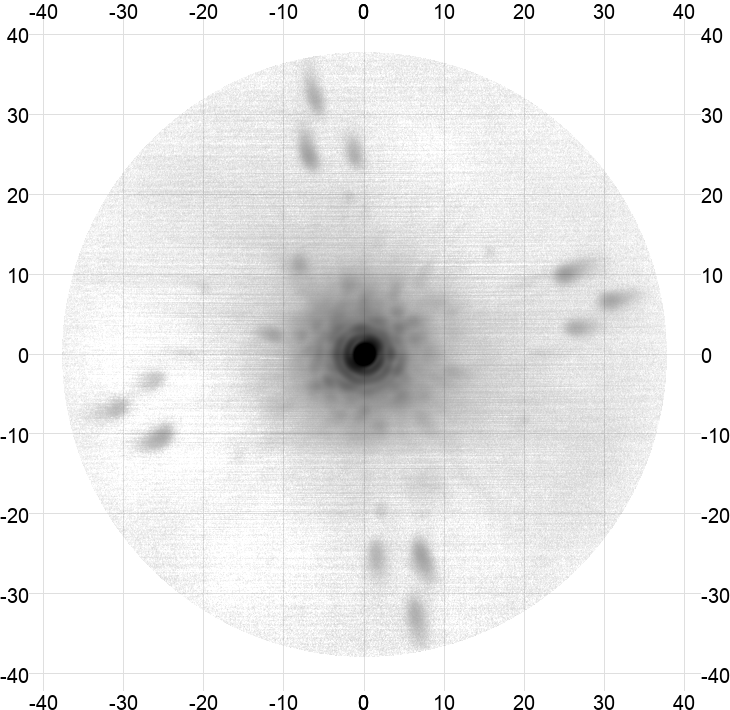 |
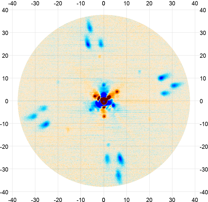 |
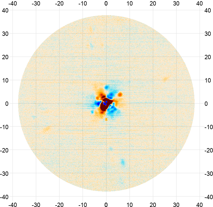 |
In total intensity the main beam dominates the center, first exhibiting Airy rings and then fragmenting into blobs as it fades away. Then, at a distance of 22–36′, a 4-way symmetric pattern of 3 near sidelobes appears, each somewhat wider than the main beam, elongated by a factor of 2–3 and with a peak amplitude of around 0.3%. These “little buddies” are probably a result of diffractive effects in the free space filters located near the Lyot Stop. These filters are constructed from multiple layers of metal mesh grids with different periodicities oriented along axes that are rotated between layers. This construction leads to a Moiré pattern with centimeter scale periodicities consistent with the observed pattern.
In and the central region shows a 3-fold T→P leakage pattern, but in terms of the regular and this is simply a dipole and will therefore mostly cancel when observations taken at different telescope orientations (e.g. rising and setting) are combined. The near sidelobes, on the other hand, are almost purely and near 100% polarized, resulting in a net T→E polarization leakage regardless of the telescope orientation, predominantly to . Overall the near sidelobes have a flux of around 0.8% that of the main beam for PA5 f150 and less for the other arrays. We do not detect them at f090 or for PA4.
B.1 Near sidelobe subtraction
With 0.8% of the main beam’s flux leaking into E-modes via the near sidelobes, they represent a small but not negligible systematic, which we handle in two stages. Firstly, we subtract an approximate model of their signal during mapmaking. Secondly, we measure the residual T→E leakage and include it in our effective beam model.
If computational resources were not a concern, the sidelobes could be deconvolved by including them in the pointing matrix, . Since we wish to solve for the sky as seen by the main beam, would include the near sidelobe pattern shown in figure 22 with the main beam deconvolved. The total would then be used in the mapmaking equation, resulting in a sidelobe-free map. But in practice this approach is much too costly, as each sample in the pointing matrix would need to touch all pixels with a significant sidelobe signal, making it hundreds of times more expensive. This expense would be incurred every time is used, which is twice per CG step, making the whole mapmaking process forbiddingly slow.
To keep things practical we make two approximations:
-
1.
Instead of including in the main pointing matrix, we use it to clean the TOD: . Here is a guess at what the sky map looks like. In our case, that’s the output map from the previous pass in the multipass mapmaking. Since the near sidelobes are an perturbation, this approximation is more than good enough.
-
2.
We approximate as a sum of 12 scaled and offset versions of the main beam, one per near sidelobe. This reduces the cost of to be 12 times that of . This is a much rougher approximation than the first, but is sufficient for our purposes given the already low level of the sidelobes.
Together, these approximations mean that the near sidelobe subtraction can be done at the cost of 6 CG steps – less than a percent of our mapmaking expenses. Figure 23 shows how this approximation compares to the actual sidelobe pattern, and what residual is left. While the residual is visually quite large, it is mostly limited to high . This approximate sidelobe subtraction succeeds in reducing the near sidelobe T→E leakage by a factor of 5 in the range where most of this leakage happens.
See Duivenvoorden et al. (in prep) for more details on the beams and the modeling and treatment of T→P leakage.
| data | model | residual |
|---|---|---|
|
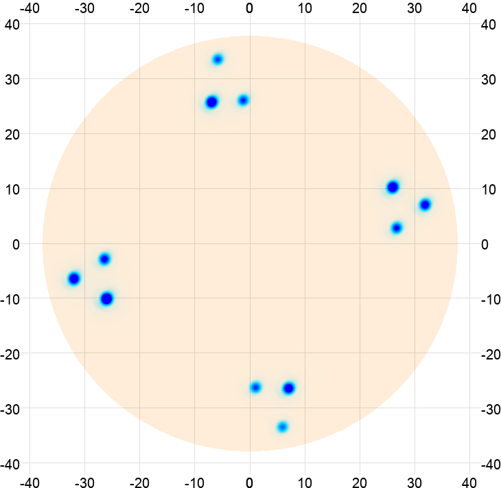 |
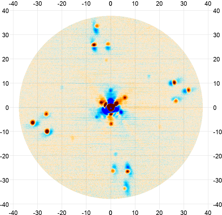 |
Appendix C Far sidelobes
We map out the far sidelobes by projecting our night-time CMB observations into Moon-centered maps and day-time CMB observations into Sun-centered maps. Only observations where the object in question is above the horizon were used. Examples of these maps are shown in figure 24. Overall these sidelobes are quite weak, with the most important ones reaching a few mK when sourced by the 6000 K Sun, corresponding to a dB suppression compared to the main beam. They are relatively extended, often covering tens of degrees in size, but can also be as narrow as the Sun and Moon allow us to resolve.
While the location and overall shape of the sidelobes are robust, the substructure depends strongly on a detector’s position in the focalplane. Detectors separated by just a few arcminutes can observe a phase shift in the substructure. This makes the sidelobes difficult to subtract, and might also be the source of the larger than expected disagreement between the Sun-centered and Moon-centered sidelobe maps in figure 24.
As when mapping the CMB, atmospheric noise makes it difficult to measure total intensity on scales larger than about a degree, and our sidelobe maps can therefore only capture the narrowest of features in total intensity. We therefore base our sidelobe analysis on the polarization maps, which have much higher S/N on large scales. No features visible in total intensity are missing in the polarized maps, indicating that all our sidelobes are strongly polarized. This is also expected physically, as the sidelobes are caused by oblique reflections off flat surfaces surrounding the main mirror Duivenvoorden et al. (in prep).
Since they’re so weak, we can safely ignore the far sidelobes unless something extremely bright hits them. We chose to mask samples where the Moon sidelobe signal is brighter than 200 µK or (for day-time observations) where the Sun sidelobe signal is brighter than 500 µK. These areas are marked with black contours in figure 24. While a 200/500 µK threshold might seem permissive compared the CMB’s µK and µK RMS in total intensity and polarization, this averages down rapidly when observations with different telescope orientations and Moon/Sun positions are combined. The residual Moon/Sun sidelobe contamination after this cut therefore ends up being a subdominant noise373737The Moon/Sun sidelobe signal is a noise source, not a bias source, because the Moon and Sun have time to move significantly between the observations that go into different parts of our data splits, meaning their signal does not add up coherently in the cross spectrum. source compared to the atmosphere.
Overall these cuts remove around 1% of the samples during the night and 5% during the day.
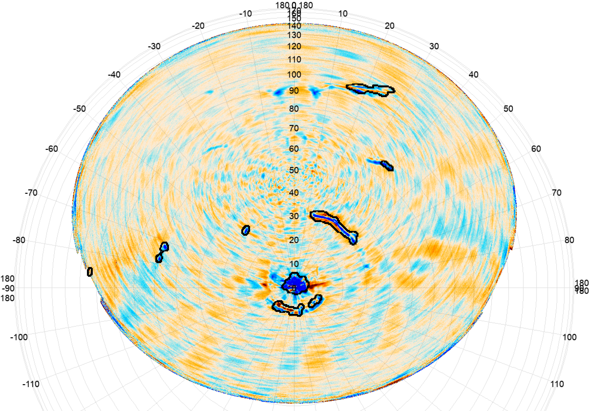
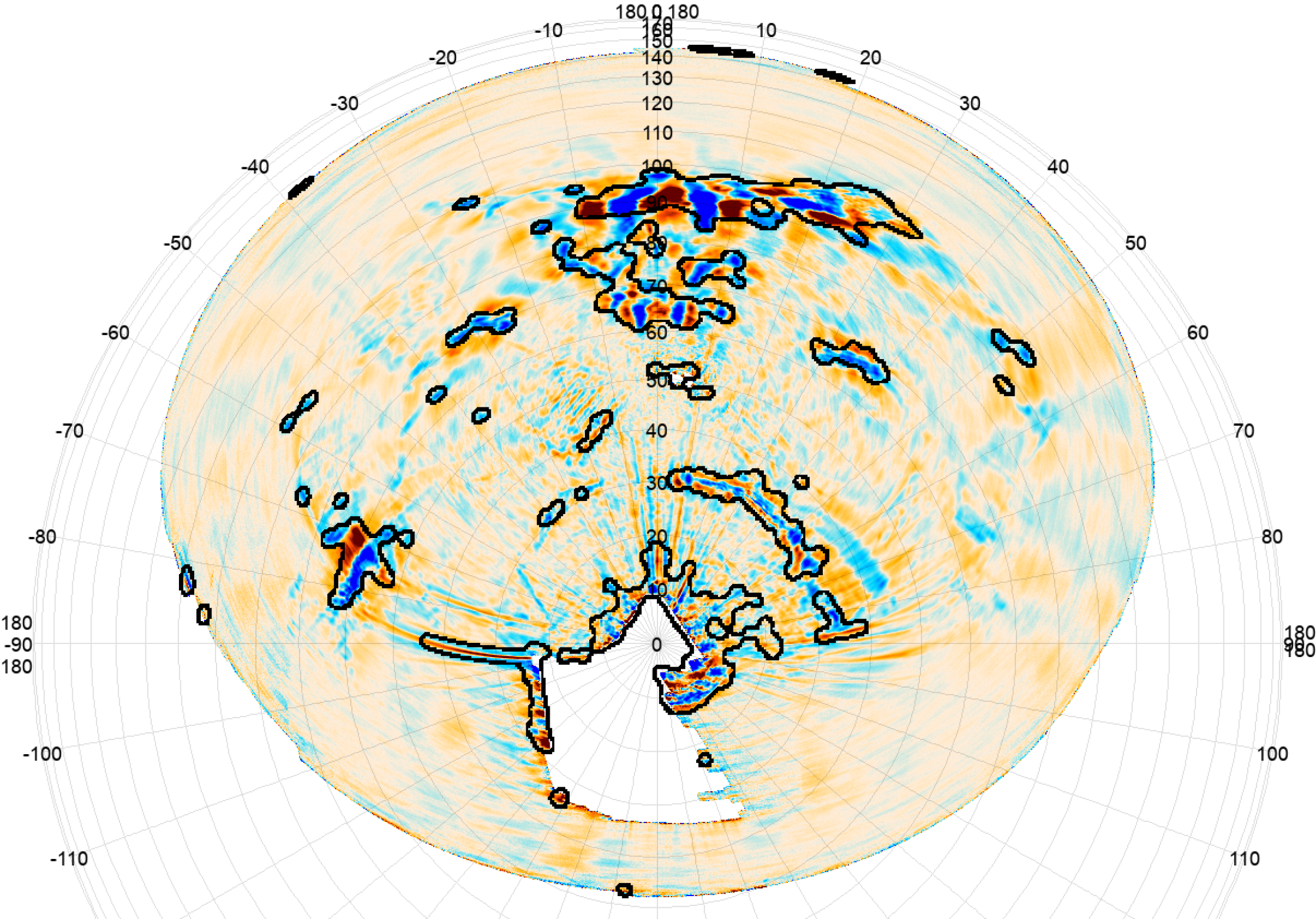
Appendix D Daytime beam
During the day, the Sun heats ACT’s primary mirror, causing it to expand and the beam to deform. This deformation depends on how much each part of the mirror or supporting structure expands, and can be quite complicated. Figure 25a shows four examples of ACT day-time beam shapes for each of the detector arrays considered in DR6. The behavior varies from no worse than the night to strongly deformed and multi-lobed.
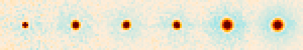
|
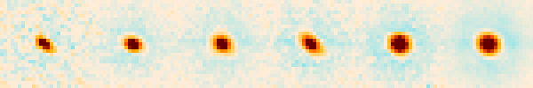
|
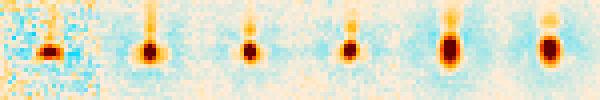
|
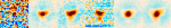
|
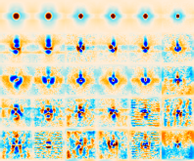
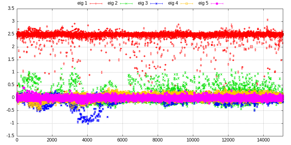
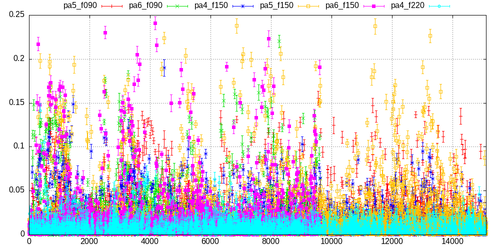
The process of constructing the per-TOD pointing model also produces a large number of point source images, which we used to find the eigenmodes for the beam variability. Most of the beam variance can be explained by the top five eigenmodes, which are shown in figure 25b. Figure 26 shows the amplitude of the eigenmodes for each such point source image, sorted by time. The first eigenmode corresponds to the ACT night-time beam, while the others represent deviations from this ideal. We can construct a badness statistic which is plotted in figure 27. This looks quite chaotic, but patterns emerge when plotted vs. both day-of-year and hour-of-day, as shown in figure 28. Most of the day-time region (11 < UTC < 23) has a relatively well-behaved beam, with relatively compact areas of badness. This becomes even more apparent when split into four groups by the central azimuth of the scan. We use this to define the following beam badness cut: For each TOD, use its date and UTC hour to look up its predicted beam badness in the azimuth-split version of figure 28, and exclude it from mapmaking if . This cut excludes 30%/34%/33% of the PA4/PA5/PA6 day-time data. The night-time data are not impacted.
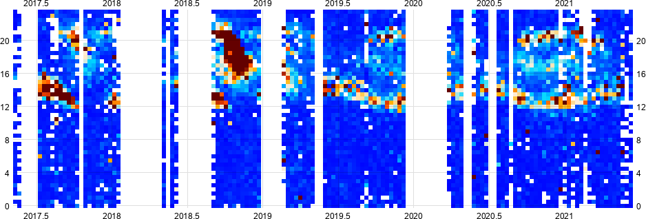
Appendix E Per-TOD pointing correction
The DR4 pointing fit was performed using a TOD-level likelihood search which was significantly more expensive than the CMB mapmaking, itself one of the heaviest steps in the whole analysis. To avoid this, DR6 uses a new pointing model that aims to be faster, higher time resolution and easier to debug by doing the pointing fit in pixel space instead of time domain. It proceeds as follows:
-
1.
Build a catalog of bright point sources with known locations. We crossmatched a preliminary catalog of 5345 point sources detected at and mJy in the first two seasons of ACT DR6 f150 data vs. bright subsets383838 Many of these catalogs are very large (e.g. hundreds of millions of objects for WISE), which would lead to a high chance of false association in the crossmatch. We therefore restrict to brighter subsets, with size given by the second number in the parentheses. This was done somewhat arbitrarily, but the details have little impact for the mJy subset of ACT sources considered here. of the following external catalogs: ALMA (1503 matches out of 3354 objects considered = 1503/3354) (ALMA, 2019), AT20G (2103/5890) (Murphy et al., 2010), CLASS (1401/14353) (Myers et al., 2003), 2MASS (12/34322) (Skrutskie et al., 2006), WISE (38/6823) (Cutri et al., 2021), HyperLEDA (117/21591) (Makarov et al., 2014), PKS (984/8265) (Wright & Otrupcek, 1996), PMN (1329/50818) (Wright et al., 1994), LQAC 6cm (1183/5340) (Souchay et al., 2015), BSC5 (8/9110) (Hoffleit & Warren, 1995), NVSS (4164/581097 (Condon et al., 1998)) and a small list of manually entered objects (7/7). After rejecting 149 non-pointlike objects and false positives we were left with 4958 objects matching at least one external catalog. The reason for only including mJy objects was that they need to be bright enough to be detectable or close to detectable in a depth-1 map, which is much shallower than our full sky maps.
-
2.
Make depth-1 maps for all the CMB observations. Depth-1 maps are more generally useful for time domain science, and are described in section 3.7. The depth-1 maps used in the pointing correction differ from those by using a rough pointing model based on planet observations from the beginning of AdvancedACT (since the final pointing model wasn’t ready yet), and by using a rotated coordinate system to save memory by minimizing the size of the bounding box. The result is a set of maps across our bands and arrays. These are generally not written to disk, but intead are passed directly to the next step. Figure 29 shows an example of such map.
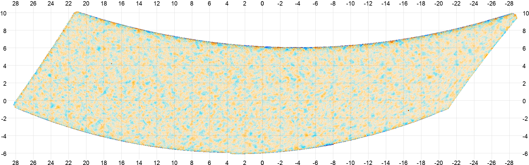
Figure 29: Example depth-1 for pointing measurement, representing around one hour of data for a single detector array. Point sources are visible as tiny red dots. Pointing errors can change significantly in one hour, but it only takes the array around 4 minutes to drift across each point in this map, so there is no appreciable pointing smearing. This plot is downsampled by a factor of 3 from its full 0.5′ resolution. Note that this map is in a different coordinate system than the standard depth-1 maps. The coordinate axes are in degrees, but do not correspond to any standard coordinates. -
3.
Extract thumbnails around each such source in each depth-1 map. See figure 30 (top) for an example of what these look like.
Figure 30: Top: thumbnails around the first 60 of the 141 point sources considered for the map in figure 29. Many of them are too faint to be seen by eye, but can still contribute to the pointing fit when modeled together. The few objects that appear to be off-center are simply bright neighbors. Bottom: Thumbnails for the same map after rotating to boresight coordinates, applying a matched filter, and cutting objects that are not at least 5 times as bright as any others within a radius of 10′. -
4.
Reject objects that are not at least 5 times as bright as the others within a 10 arcminute radius since the pointing fit assumes isolated sources.
-
5.
Rotate to the boresight coordinate system where we define our pointing offsets and apply a matched filter to maximize S/N. Coadd the matched filter maps for the two bands of each detector array, since an array’s pointing offset should be frequency-independent. This is illustrated in figure 30 (bottom).
-
6.
Do a preliminary fit of the position and flux of each object. For objects detected at use the ACT catalog flux instead of the one measured here. Using this flux, measure the objects’ S/N. Objects with are fit individually. Other objects are grouped with others observed close in time until their combined S/N exceeds 8.
-
7.
Fit the position of each group, resulting in several measurements of the horizontal and vertical pointing offsets per array per TOD. An example of this is shown in figure 31. We see a strong time-of-day dependence for the pointing offset: During the night (roughly 23-11 UTC) the pointing is relatively stable, but during the day (roughly 11-23 UTC) it fluctuates with an amplitude of around 3 arcminutes.
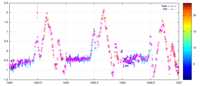
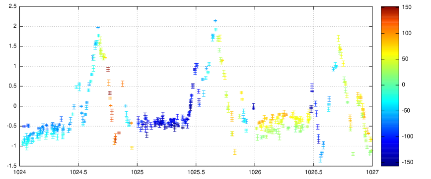
Figure 31: Top: Measured vertical pointing displacement, in arcminutes, as a function of time, in days since 2017-01-01. The points are colored by the UTC hour, with 11-23 being the rough day-time period. The magenta points show the result of the DR4 method for comparison. These have smaller error bars but lower time resolution due to averaging over all sources in a TOD. This averaging also masks the azimuth-dependent pointing offset, which we were not aware of in DR4. Bottom: The same data, this time colored by azimuth. The high scatter for is strongly correlated with azimuth. New compared to DR4 is a surprising amount of short-term scatter even during the night, with a peak-to-peak amplitude of up to 0.5′. This scatter turns out to be strongly correlated with azimuth, and was not discovered in DR4 because we didn’t have sub-TOD resolution. The pointing offset measured in DR4 was the average over all the sources inside that TOD, some of which would have had low and some high azimuth. DR4 therefore had an uncorrected pointing offset of up to 0.25′ at the ends of its widest scans. In practice this was not a big concern there because 1) the offset would usually be less than 0.25′ at the ends, 2) the average offset inside a scan would be about half that at the edges, 3) when averaging across multiple observations it adds in quadrature to the effective beam, 4) only a small subset of the DR4 data (2016 only) used as wide scans as these, and 5) we measure an empirical beam correction factor from the final maps that would absorb this. Even if all the TODs has been maximally affected by this, the expected increase in beam size at f150 would be just 0.4%.
-
8.
Both because the pointing offset varies within a TOD (due to the azimuth effect) and because a TOD in some cases has no usable measurements due to a lack of bright point sources, we can’t use these measurements directly to correct the pointing. We instead fit a smooth model that can be interpolated for each az and TOD. We build a separate model for the data points from each depth-1 map, with each model consisting of a piecewise linear function in time plus a constant slope in azimuth. This is done both for the vertical and horizontal pointing offset, for a total of free parameters per depth-1 map. We adjust to minimize , where is the number of data points from the depth-1 map and is the duration they span. Typically we end up with data points per degree of freedom in the fit.
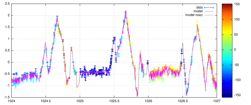
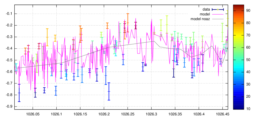
Figure 32: Top: The best-fit pointing model (magenta) compared to the same measurements as in figure 31, again with the vertical pointing offset in arcminutes on the y axis, days since 2017-01-01 on the x axis and azimuth in degrees in the colorbar. The model successfully captures both the time- and azimuth-dependence of the pointing. It is easiest to see around day 1026, where the azimuth-dependence is particularly strong. It can be hard distinguish in regions with low azimuth-dependence. The gray curve shows the model with the azimuth-dependence disabled. Bottom: Zoom in on the messy region , illustrating how the model captures the apparent scatter. The model appears to jump erratically up and down here, but this is simply a consequence of each point having its own azimuth – the model would look smooth if plotted in a 3D time-az-displacement graph. The resulting model is plotted in figure 32.
-
9.
For each TOD in DR6, evaluate the model at the TOD’s halfway time, resulting in a vertical and horizontal pointing offset along with a vertical and horizontal azimuth slope. The latter enter into a correction of the horizontal coordinate system as
(E1) where are the corrected versions of respectively, and is the azimuth of the mid-point of the scan for this TOD. Figure 33 tests the round-trip performance of the pointing correction by measuring the pointing offsets from new depth-1 maps built after applying the pointing correction. The new pointing model has similar scatter as the old DR4, but fewer outliers due to capturing the azimuth slope.
The pointing slope is similar to the effect of a tilt of the telescope’s azimuth axis from the vertical, but cannot be explained that way because it is not constant in time. We have so far not gotten to the bottom of what causes it.
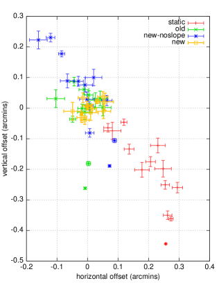
Overall the DR6 pointing model is a moderate improvement over the DR4 pointing model, but this is countered by DR6 having a much higher fraction of high-amplitude azimuth scans that are more difficult to model. As described in section 2.7, the beam size inferred from point sources in our CMB maps is slightly larger than that directly measured from planet observations. If interpreted as being entirely due to uncorrected pointing jitter, then DR6 has an average jitter of arcmin, compared to for DR4, so it’s around 30% worse.
Appendix F Spatially dependent noise
The atmosphere acts as a strongly spatially and temporally correlated noise component for ground-based CMB telescopes like ACT. When projected onto the sky via the telescope scanning pattern, this results in a map where not just the overall noise level is spatially dependent (as shown in figure 5), but also the correlation length, directions of stripiness, and so on.
One way of visualizing this by splitting the sky into tiles, and measuring the 2D noise power spectrum for each. These 2D noise spectra are shown in figure 34. The dominant feature here is the low- atmospheric noise, which is much more prominent in total intensity than in polarization. From this central peak two thin lines of higher noise power extend outwards in a strongly declination-dependent X-shape along the two dominant scanning directions. Unexpectedly, this X-shape has similar width and amplitude for polarization and total intensity, but that amplitude is low enough, at around two times the white noise floor, that it can probably be ignored in most contexts.
The symmetric part of the total intensity and polarization noise spectra are shown in figures 35 and 36 respectively. The spectra roughly follow the 1/f profile , with , but there are some clear deviations. At the TT noise spectrum turns over due to the mapmaker transfer function, and in polarization the slope steepens below for some of the arrays. The different tile spectra are quite consistent in TT. In EE, on the other hand, there is a strong declination dependence with up to ten times higher noise at low in the non-crosslinked region .
Figure 15 compares the tile-averaged noise spectra for the different detector arrays. The TT noise spectra behave as expected, getting progressively more atmospheric noise as we go to shorter wavelengths, and with the arrays being consistent with each other for each bandpass. The situation is more complicated in polarization. Here individual array differences dominate, with PA6 f090 having significantly less correlated noise than PA5 f090, and both bands of PA4 having much more correlated noise for than the other arrays.
Figures 37 and 38 show the spatial distribution of , measured as the point where the symmetric part of the noise spectrum falls below twice the noise floor. Aside from some edge areas with very few observations, the variations are declination-dominated, though there is also some RA-dependence in total intensity. Figure 39 shows the average as a function of declination, and here we again see the qualitatively different behavior in total intensity and polarization. In total intensity is mainly a function of bandpass, while in polarization is depends strongly on the detector array and crosslinking angle. In the extreme case of PA4 f220 is more than 3 times as high at as at .
The inconsistent behavior of the correlated noise in polarization is consistent with this noise being sourced by array-dependent T to P leakage. We suspect that relative gain miscalibration is the main culprit, as it has already been implicated in causing the low- power loss in the mapmaker transfer function. The difference in between PA5 f090 and PA6 f090 gives a lower bound on the noise improvements that would be possible with better calibration, but the total room for improvment is probably much greater.
It is hard to improve on this in practice for the ACT data. We perform regular bias steps, but these have proven to be even less reliable for relative gain calibration than the atmospheric common mode calibration we currently use. In theory it would be possible to solve for the per-detector gains jointly with the sky map. We have tested this for small toy examples, but we know of no algorithm that can solve this in reasonable time for realistic data sets.
ACT’s successor, the Simons Observatory Large Aperture Telescope, should improve on this situation by having a built-in optical stimulator that will provide frequent calibration, though even this approach is vulnerable to percent-level bandpass mismatch between different detectors.
See Atkins et al. (2023) for more in-depth discussion of the noise properties of the ACT maps.
TT
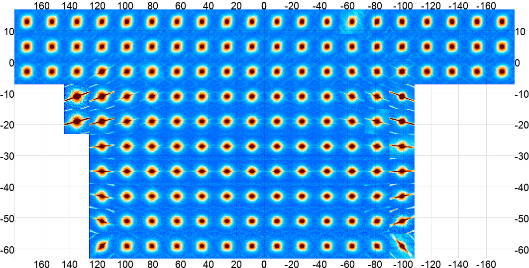
EE
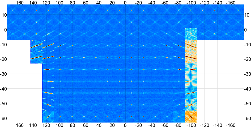
| PA5 f090 | PA6 f090 |
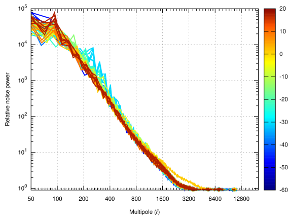 |
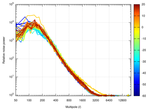 |
| PA5 f150 | PA6 f150 |
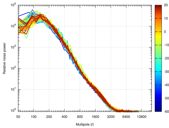 |
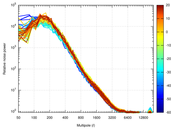 |
| PA4 f150 | PA4 f220 |
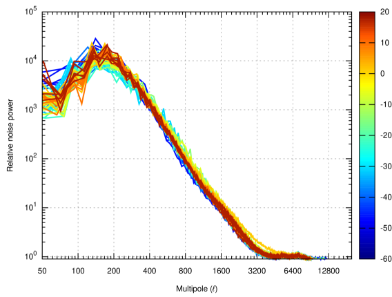 |
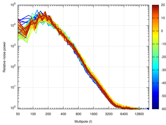 |
| PA5 f090 | PA6 f090 |
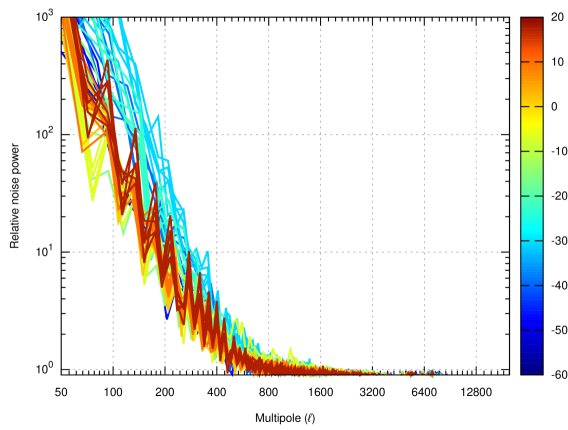 |
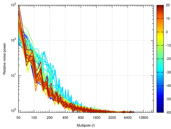 |
| PA5 f150 | PA6 f150 |
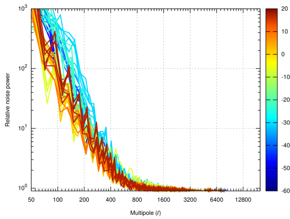 |
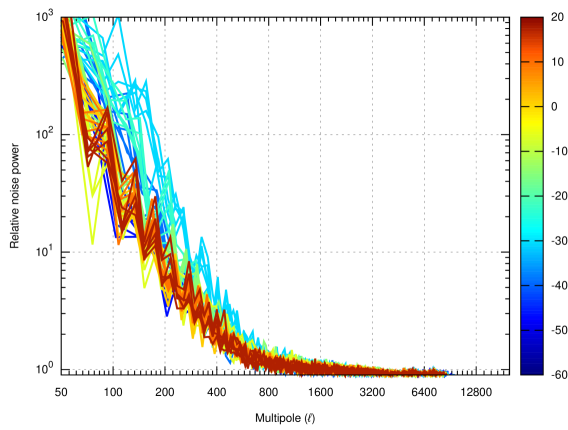 |
| PA4 f150 | PA4 f220 |
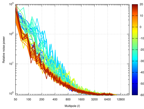 |
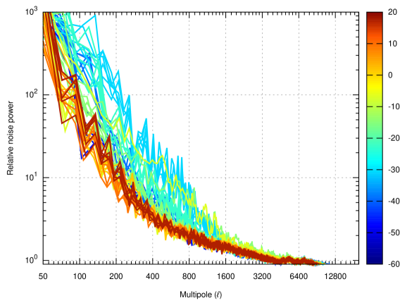 |
| PA5 f090 | PA6 f090 |
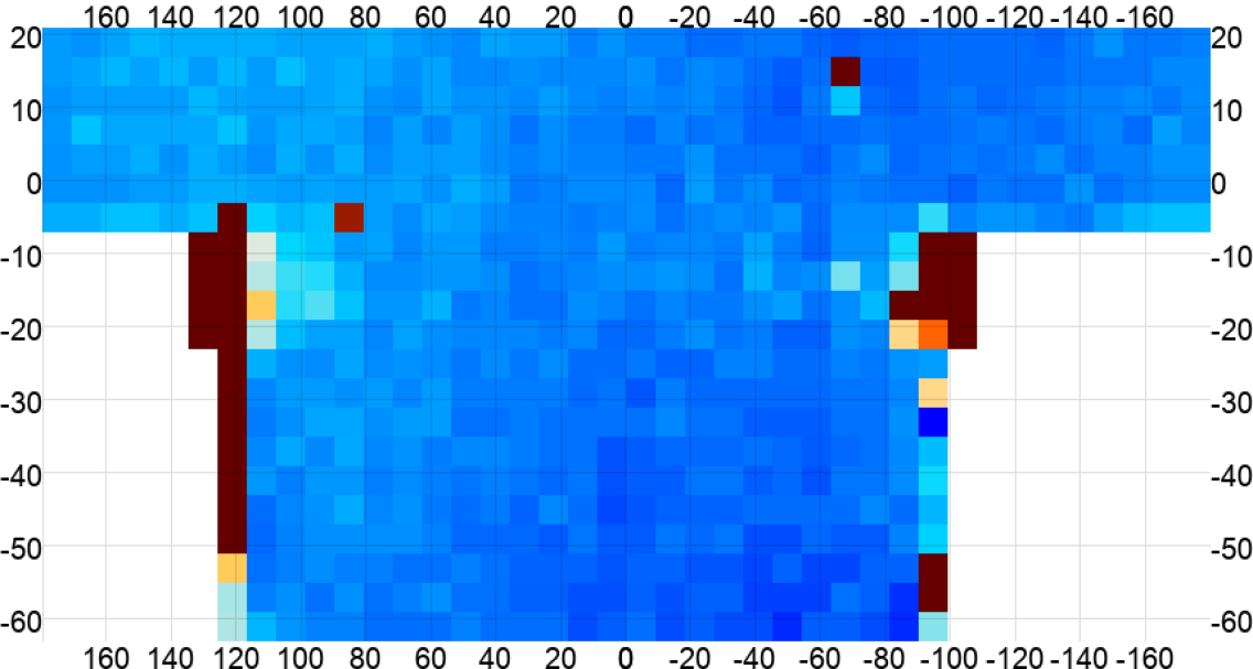 |
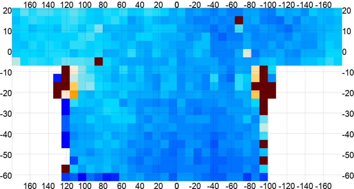 |
| PA5 f150 | PA6 f150 |
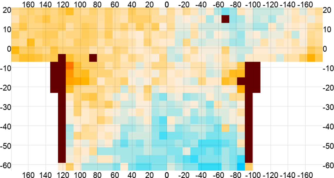 |
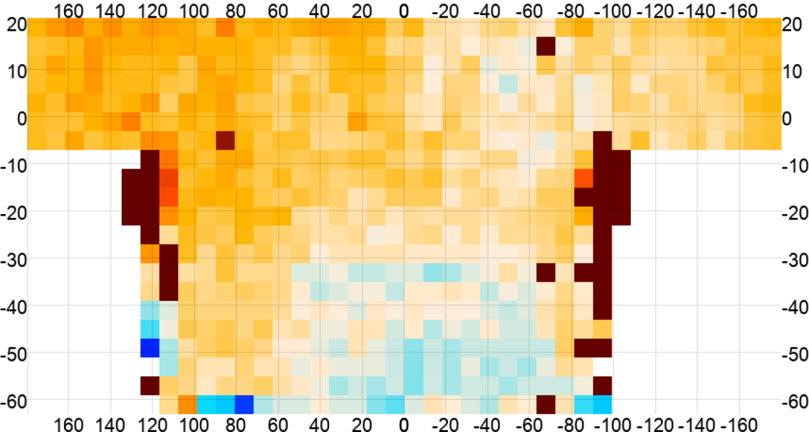 |
| PA4 f150 | PA4 f220 |
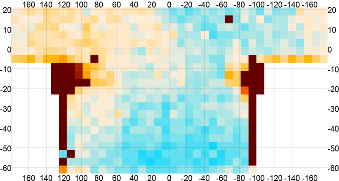 |
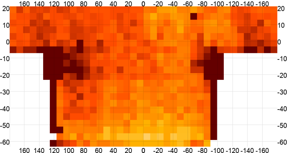 |
| PA5 f090 | PA6 f090 |
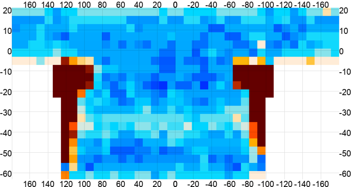 |
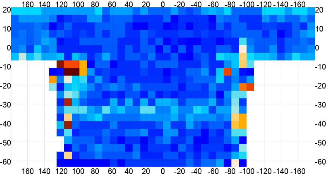 |
| PA5 f150 | PA6 f150 |
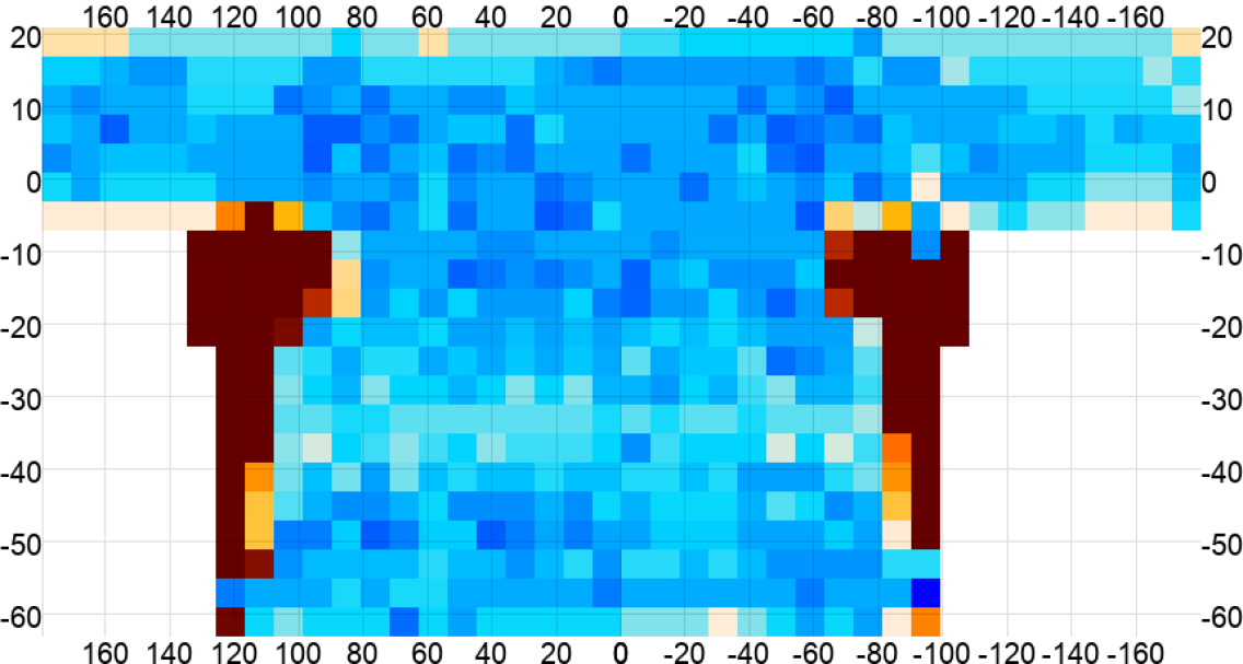 |
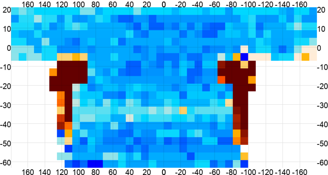 |
| PA4 f150 | PA4 f220 |
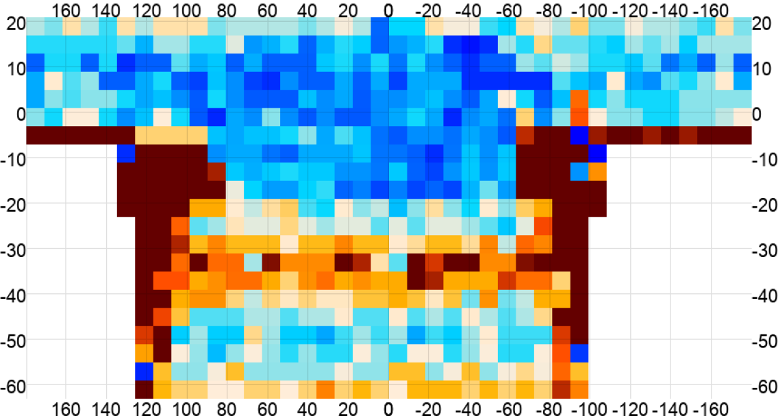 |
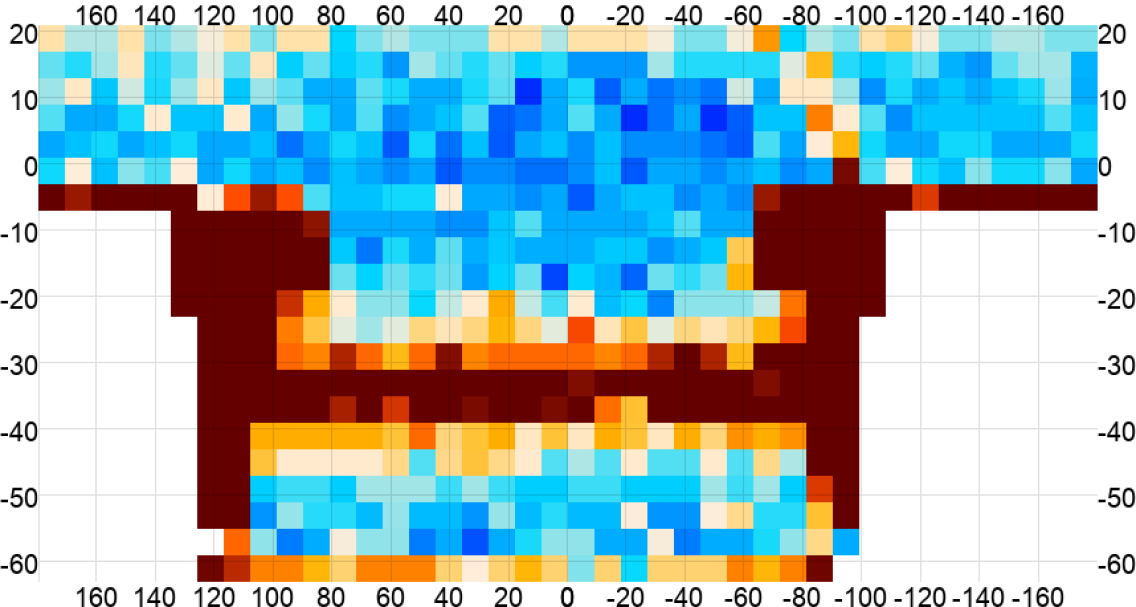 |
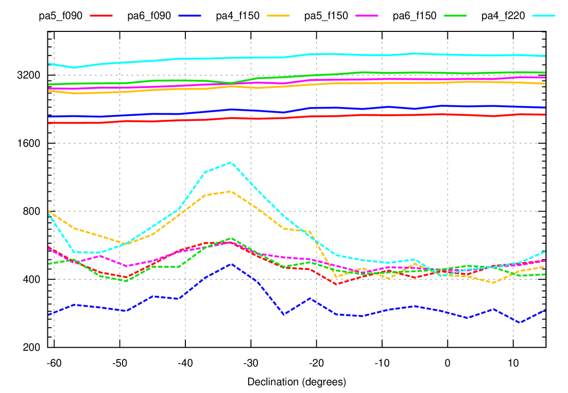
Appendix G Transfer function and
To illustrate the different scale-dependence of and in equation 14, we implemented a simple 1D toy example consisting of 900 samples scanning at constant speed across 300 pixels. We considered two cases.
-
1.
The true instrument response is given by a linear interpolation pointing matrix while the analysis is done assuming a nearest neighbor pointing matrix. This mismatch results in sub-pixel model errors.
-
2.
Both use nearest neighbor (so there is no sub-pixel mismatch in this case), but each row of the pointing matrix used for the analysis is scaled by 0.9 for even samples and 1.1 for odd samples, representing gain miscalibration. These rapid gain changes emulate the effect of multiple detectors with relative gain errors observing the same spot in the sky in rapid succession.
The results are shown in figure 40, and show that has a shallower scale dependence than . This means that it can be negligible on small scales while still being important at large scales. The figure also shows that
| (G1) |
from equation 14 is a good approximation for the transfer function. We recognize the general behavior from figure 17. The nearest neighbor transfer function turns on more gradually than the gain error transfer function, consistent with the smaller slope difference between and for that case.
| Nearest neighbor subpixel errors | Relative gain errors |
|---|---|
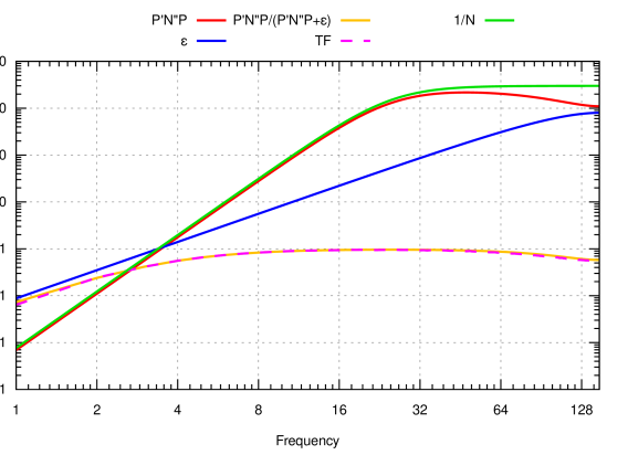 |
See Naess & Louis (2023) for more detailed discussion about model error induced transfer functions in CMB mapmaking, including how it affects all mapmaking methods, not just maximum-likelihood.
Appendix H Peak stacking
We produced the stacks in figures 10 and 11 by first finding peaks in a reference map (e.g. the E-mode map when stacking on E), and then stacking the target map on these locations. We considered four data sets:
-
1.
Planck: Planck 2018 SMICA CMB-only maps
-
2.
ACT: A naive, per-pixel inverse variance weighted coadd of ACT DR6 point source subtracted night-only f090 and f150 maps with no beam reconvolution. The effective beam is an average of the f090 and f150 beams, Beam details on this scale have negligible impact on the stack plots.
-
3.
ACT+Planck: Naive, per-pixel inverse variance weighted coadd of the point source subtracted f090 and f150 ACT+Planck coadd maps. Similar beam as ACT-only.
-
4.
Simulation: A beam-free, noiseless simulation.
The same data set was used both for peak finding and peak stacking, e.g. when stacking ACT+Planck E on T, peak-finding was done on ACT+Planck E, and ACT+Planck T was then stacked on these locations.
H.1 Peak finding
We find peaks by masking high-foreground and high-noise regions,
apodizing the edge by , and low-pass filtering to
remove noise-dominated modes. We then found local maxima and
minima as using scipy.ndimage.maximum_filter and
scipy.ndimage.minimum_filter with a 2-pixel radius
circular footprint. We label these as “positive” and “negative”
peaks respectively.393939This refers to the sign of a peak
relative to its local surroundings, not the absolute value of the
map at this spot. The band-pass filter was a Butterworth
profile
| (H1) |
For ACT and the simulation, we used an of 3000/2000 for T/E, while for Planck we used 2000/800 due to lower S/N. No beam deconvolution was performed. The result was a list of around 300 000 peaks in T and 450 000 peaks in E.
H.2 Peak stacking
We apply the same mask to the map to stack. For each peak, we reproject a thumbnail around it to RA=, dec= using non-uniform FFT interpolation404040 When interpolating it’s important that there’s at least one output pixel for every input pixel to avoid losing information. The maximal resolution in the input map is , so we reproject to resolution. while taking into account the per-pixel polarization angle rotation caused by the parallel transport. We define the positive/negative stack map as the plain, unweighted average of the positive/negative reprojected thumbnails. The full stack map is then
| (H2) |
This stack map suffers from large-scale horizontal striping with two causes:
-
1.
The ACT-only map contains horizontal stripes from azimuth-synchronous pickup (see figure 20).
-
2.
The ACT+Planck map lacks power for due to a pickup filter applied to the ACT contribution to the coadd. This results in a bias towards detecting positive peaks in areas with mostly negative signal on the same declination. When stacking even an unfiltered map using these peaks, the result is a negative horizontal stripe around a stack on positive peaks.
These horizontal stripes are a distraction from the baryon-acoustic osciallation physics the stacks illustrate, so we remove them by subtracting the average value in each row of the map, excluding the region to avoid biasing the BAO signal itself.
For plotting purposes, we convert the linear polarization Stokes parameters Q and U into E and B. We also show the related quantities and , which are Simply Q and U defined relative to the stacking center instead of the North pole (Kamionkowski et al., 1997).
Finally, we normalize each plot T plot by dividing it by the 95% quantile of the absolute value of the T signal for . Similarly, and are normalized using and E and B using E.