Approximation of diffeomorphisms for quantum state transfers

Abstract.

In this paper, we seek to combine two emerging standpoints in control theory. On the one hand, recent advances in infinite-dimensional geometric control have unlocked a method for controlling (with arbitrary precision and in arbitrarily small times) state transfers for bilinear Schrödinger PDEs posed on a Riemannian manifold $M$. In particular, these arguments rely on controllability results in the group of the diffeomorphisms of $M$. On the other hand, using tools of $\Gamma$-convergence, it has been proved that we can phrase the retrieve of a diffeomorphism of $M$ as an ensemble optimal control problem. More precisely, this is done by employing a control-affine system for simultaneously steering a finite swarm of points towards the respective targets. Here we blend these two theoretical approaches and numerically find control laws driving state transitions (such as eigenstate transfers) in a bilinear Schrödinger PDE posed on the torus. Such systems have experimental relevance and are currently used to model rotational dynamics of molecules, and cold atoms trapped in periodic optical lattices.

1. Introduction

1.1. The Schrödinger equation

In this work we study bilinear Schrödinger PDEs of the type

$$\begin{cases}i\partial_{t}\psi(t,x)=\left(-\Delta+V(x)+\sum_{j=1}^{m}u_{j}(t)W_{j}(x)\right)\psi(t,x),&\\ \psi(0,\cdot)=\psi_{0},\end{cases}$$ (1.1)

with $(t,x)\in(0,T)\times M$, where $M$ is a smooth connected boundaryless Riemannian manifold, $\Delta$ is the Laplace-Beltrami operator of $M$, the potentials $V,W_{1},\dots,W_{m}\colon M\to{\mathbb{R}}$ and the controls $u_{1},\dots,u_{m}\colon[0,T]\to{\mathbb{R}}$ are real valued functions. The uncontrolled operator $-\Delta+V$ is referred to as the drift. Equation (1.1) describes an infinite-dimensional non-linear control-to-state system. By choosing a locally integrable control signal $u=(u_{1},\dots,u_{m})$ and picking up an initial state $\psi_{0}$ in the unit sphere

$$\mathcal{S}\coloneqq\{\psi\in L^{2}(M,{\mathbb{C}})\,\mid\|\psi\|_{L^{2}}=1\},$$ (1.2)

$\psi(t;u,\psi_{0})$ denotes (if well-defined) the solution of (1.1) at time $t\geq 0$.

System (1.1) models a quantum particle on $M$, with free energy $-\Delta+V$, interacting with external potentials $W_{j}$, which can be switched on and off. This framework models a variety of physical situations, such as atoms in optical cavities [19], and molecular dynamics [13].

We are interested in the approximate controllability of (1.1).

Definition 1.

• The state $\psi_{1}\in\mathcal{S}$ is said to be approximately reachable from $\psi_{0}\in\mathcal{S}$ for (1.1) if, for every $\varepsilon>0$, there exist a time $T\geq 0$, a global phase $\theta\in[0,2\pi)$ and a control $u\in L^{1}_{\rm loc}([0,T],{\mathbb{R}}^{m})$ such that

  $$\|\psi(T;u,\psi_{0})-\psi_{1}e^{i\theta}\|_{L^{2}}<\varepsilon.$$

• The state $\psi_{1}\in\mathcal{S}$ is said to be small-time approximately reachable from $\psi_{0}\in\mathcal{S}$ for (1.1) if, for every $\varepsilon>0$, there exist a time $\tau\in[0,\varepsilon]$, a global phase $\theta\in[0,2\pi)$ and a control $u\in L^{1}_{\rm loc}([0,\tau],{\mathbb{R}}^{m})$ such that

  $$\|\psi(\tau;u,\psi_{0})-\psi_{1}e^{i\theta}\|_{L^{2}}<\varepsilon.$$

We shall also say that (1.1) is (small-time) approximately controllable if the set of (small-time) approximately reachable operators coincides with $\mathcal{S}$ from any $\psi_{0}\in\mathcal{S}$.

This problem has been widely investigated by control theorists in the last three decades, due to its relevance in applications to physics and chemistry (e.g. absorption spectroscopy, and NMR pulse design) [11, 14], or computer science (e.g. error correction for robust quantum computation) [12, 3]. E.g., if the drift $-\Delta+V$ has compact resolvent (hence purely point spectrum), (1.1) is known to be approximately controllable generically w.r.t. the potentials $V,W_{1},\dots,W_{m}\in L^{\infty}(M,{\mathbb{R}})$ [17]. The first examples of small-time approximately controllable Schrödinger equations of the form (1.1) were obtained only recently in [5].

In this article, we study a particular example of Schrödinger equation of the form (1.1).

1.2. An equation posed on $M={\mathbb{T}}^{d}={\mathbb{R}}^{d}/2\pi{\mathbb{Z}}^{d}$.

We consider the Schrödinger equation of the form (1.1) with

$$\begin{split}&M={\mathbb{T}}^{d},\quad m=2d,\quad V\in L^{\infty}({\mathbb{T}}^{d},{\mathbb{R}}),\\ &W_{2j-1}(x)=\sin\langle b_{j},x\rangle,\quad W_{2j}(x)=\cos\langle b_{j},x\rangle,\quad j=1,\dots,d,\\ &b_{1}=(1,0,\dots,0),\quad b_{2}=(0,1,\dots,0),\quad\dots\\ &b_{d-1}=(0,\dots,1,0),\quad b_{d}=(1,\dots,1).\end{split}$$ (1.3)

When $d=1$, this setting models the rotational motion of a rigid molecule whose dynamics are confined to a plane, controlled by two orthogonal lasers (of constant direction and tunable amplitude) coupled to its dipolar moment (see, e.g., the recent physical review [15] and the references therein). It also describes a (linear-in-state) Bose-Einstein condensate in a $d-$dimensional optical lattice with tunable depth and phase [9].

The approximate controllability of system (1.1)-(1.3) in $d=1$ was established in [6] with finite-dimensional Galerkin approximations and averaging techniques. The small-time approximate controllability of (1.1)-(1.3) (in any dimension $d$), which had remained an open question for a decade [7], was also recently established in [4] with completely different techniques, inspired by an infinite-dimensional geometric control approach introduced in [8].

1.3. Our contribution

Small-time approximate controllability of (1.1)-(1.3) implies the theoretical capability of driving state transfers in arbitrarily small times (with the flaw of using of course controls with unbounded amplitudes). These results shed light on the theoretical and practical problem of quantum speed limit. Unfortunately, the technique developed in [4] does not provide explicit control laws for achieving state transitions, but it only ensures the existence of such controls. In other words, in a crucial passage of the proof, the explicit character of the control is lost and only existence can be asserted. More precisely, this happens when invoking a celebrated diffeomorphism decomposition result: given a diffeomorphism $P\in{\rm Diff}^{0}({\mathbb{T}}^{d})$ isotopic to the identity, owing to the simplicity of the group ${\rm Diff}^{0}({\mathbb{T}}^{d})$ established by Thurston [26], there exists $n\in{\mathbb{N}}$ and vector fields $f_{1},\dots,f_{n}\in{\rm Vec}({\mathbb{T}}^{d})$ such that

$$P=\Phi^{1}_{f_{n}}\circ\cdots\circ\Phi^{1}_{f_{1}},$$

where $\Phi^{t}_{f}$ denotes the flow at time $t$ of the vector field $f$. In general, given $P\in{\rm Diff}^{0}({\mathbb{T}}^{d})$, it is highly nontrivial to guess the number $n$ and the vectors $f_{1},\dots,f_{n}$ for which such a decomposition holds. Let us now assume that we are given a finite family of vector fields $g_{1},\ldots,g_{k}\in{\rm Vec}({\mathbb{T}}^{d})$ whose flows composition generates approximately the group ${\rm Diff}^{0}({\mathbb{T}}^{d})$ (such a family exists, see e.g. [2, Theorem 6.6]). Then, the problem of approximating $P$ with these flows turns out to be a control problem with infinite-dimensional state space, i.e., ${\rm Diff}^{0}({\mathbb{T}}^{d})$.

In this article, our aim is to numerically compensate for this lack of constructiveness by showing that the explicit character of the control can be recovered through an approximation procedure.

The idea of using flows of control-affine systems for diffeomorphism approximation was proposed by [2], and it has been a cornerstone for recent developements on the mathematical foundations of Machine Learning [25, 1]. Here, we pursue an approach similar to that proposed in [22]. That is, the diffeomorphism approximation task was formulated as an infinite-dimensional optimal control problem in ${\rm Diff}^{0}({\mathbb{R}}^{d})$. Moreover, aiming to have a numerically tractable problem, in [22] the author employed $\Gamma$-convergence arguments for reducing the original infinite-dimensional state space setting to an optimal control problem concerning the simultaneous steering of a finite (large enough) ensemble of points.

For the sake of simplicity, here we design explicit control laws for $d=1$, and for specific but relevant state transfers of (1.1)-(1.3) (namely, from the ground to one of the first excited states, and from the ground to a highly oscillating state). However, similar methods could in theory be applied in any dimension $d$ and for arbitrary state transfers.

2. From controlled Schrödinger equation to diffeomorphisms control

In order to simplify the exposition, we shall study the following Schrödinger equation on ${\mathbb{T}}$:

$$i\partial_{t}\psi(t,x)= \big{(}-\partial^{2}_{x}+V(x)+u_{1}(t)\cos(x)+u_{2}(t)\sin(x)+$$

$$u_{3}(t)\cos(2x)+u_{4}(t)\cos(4x)\big{)}\psi(t,x),$$ (2.1)

but we remark the same conclusion (namely, Theorem 2.1 below) actually holds with two controls only $u_{1},u_{2}$ (i.e., with $u_{3},u_{4}\equiv 0$), as shown in [4], which corresponds exactly to the system (1.1)-(1.3) for $d=1$. We consider the following product formula for $\tau>0$ and $\varphi\in C^{\infty}({\mathbb{T}},{\mathbb{R}})$

$$e^{i\frac{\varphi}{2\tau}}e^{i(\Delta-V)}e^{-i\frac{\varphi}{2\tau}}=\exp\left(i\tau(\Delta-V)+\mathcal{T}_{\nabla\varphi}+i\frac{|\nabla\varphi|^{2}}{4\tau}\right),$$

where $f\mapsto\mathcal{T}_{f}$ is defined as

$$\mathcal{T}_{f}\coloneqq\langle f,\nabla\cdot\rangle+\frac{1}{2}{\rm div}(f),$$

and it is a first-order self-adjoint differential operator on $L^{2}({\mathbb{T}},{\mathbb{C}})$ with domain $H^{1}({\mathbb{T}},{\mathbb{C}})$. Hence, by the Trotter-Kato product formula [21, Theorem VIII.31], we have that

$$\left(e^{i\frac{|\nabla\varphi|^{2}}{4n\tau}}e^{i\frac{\varphi}{2\tau}}e^{i\frac{\tau}{n}(\Delta-V)}e^{-i\frac{\varphi}{2\tau}}\right)^{n}\underset{n\to\infty}{\longrightarrow}e^{i\tau(\Delta-V)+\mathcal{T}_{\nabla\varphi}}$$ (2.2)

strongly (i.e., tested on any $\psi_{0}\in L^{2}({\mathbb{T}},{\mathbb{C}})$, and in the $L^{2}$-norm). Moreover, owing to [20, Theorem VIII.21 & Theorem VIII.25(a)], the following strong convergence holds as well:

$$e^{i\tau(\Delta-V)+\mathcal{T}_{\nabla\varphi}}\quad\underset{\tau\to 0}{\longrightarrow}\quad e^{\mathcal{T}_{\nabla\varphi}}.$$

Then, we consider $\varphi(x)=\cos(x)$, and we notice that

$$|\nabla\varphi|^{2}=\sin^{2}(x)=\frac{1-\cos(2x)}{2}.$$

Analogously, we take $\varphi(x)=\sin(x)$ and we observe that

$$|\nabla\varphi|^{2}=\cos^{2}(x)=\frac{1+\cos(2x)}{2}.$$

Since $\cos(x),\cos(2x),\cos(4x)$ are all control operators appearing in (2.1), the following states

$$e^{\mathcal{T}_{u\sin(x)\partial_{x}}}\psi_{0},e^{\mathcal{T}_{v\cos(x)\partial_{x}}}\psi_{0},e^{\mathcal{T}_{w\sin(2x)\partial_{x}}}\psi_{0},\quad u,v,w\in{\mathbb{R}},$$

are small-time approximately reachable from any $\psi_{0}\in L^{2}({\mathbb{T}},{\mathbb{C}})$. Therefore, by the Trotter-Kato product formula,

$$\left(e^{\frac{-1}{tn}\mathcal{T}_{f}}e^{-t\mathcal{T}_{g}}e^{\frac{1}{tn}\mathcal{T}_{f}}e^{t\mathcal{T}_{g}}\right)^{n}\!\!\!\!\!\!\underset{n\to\infty}{\longrightarrow}\!\!\exp\left(\frac{-1}{t}\mathcal{T}_{f}+e^{-t\mathcal{T}_{g}}\frac{1}{t}\mathcal{T}_{f}e^{t\mathcal{T}_{g}}\right)$$ (2.3)

and by [4, Lemma 26]

$$\exp\left(\frac{-1}{t}\mathcal{T}_{f}+e^{-t\mathcal{T}_{g}}\frac{1}{t}\mathcal{T}_{f}e^{t\mathcal{T}_{g}}\right)\underset{t\to 0}{\longrightarrow}e^{\mathcal{T}_{[f,g]}},$$ (2.4)

where the above limits are in the strong sense. Since

$$[\cos(x)\partial_{x},\sin(x)\partial_{x}]=\partial_{x},$$

we also get that the states

$$e^{\mathcal{T}_{s\partial_{x}}}\psi_{0},s\in{\mathbb{R}},$$

are small-time approximately reachable from any $\psi_{0}$. Notice that, by the method of characteristics and Liouville formula,

$$\left(e^{t\mathcal{T}_{f}}\psi\right)(x)=|D_{x}\Phi_{f}^{t}(x)|^{1/2}\,\psi\big{(}\Phi_{f}^{t}(x)\big{)}=e^{\frac{1}{2}\int_{0}^{t}{\rm div}f(\Phi_{f}^{s}(x))\,\mathrm{d}s}\,\psi\big{(}\Phi_{f}^{t}(x)\big{)},$$

where we used the abbreviation $|D_{x}\Phi_{f}^{t}(x)|\coloneqq\det D_{x}\Phi_{f}^{t}(x)$ for the determinant of the Jacobian. At this point, it is convenient to define the following fields

$$g_{0}(x)\coloneqq\partial_{x},\,\,g_{1}(x)\coloneqq\sin(x)\partial_{x},\,\,g_{2}(x)\coloneqq\sin(2x)\partial_{x}$$ (2.5)

for every $x\in{\mathbb{T}}$. We have the following result.

Theorem 2.1.

For any $P\in{\rm Diff}^{0}({\mathbb{T}}),\psi_{0}\in L^{2}({\mathbb{T}},{\mathbb{C}})$, the state $|DP|^{1/2}(\psi_{0}\circ P)$ is small-time approximately reachable for (2.1).

Proof.

By [2, Theorem 6.6], for any $f\in{\rm Vec}({\mathbb{T}})$ there exists $\{f_{n}\}_{n\in{\mathbb{N}}}\subset{\rm Lie}\{g_{0},g_{1},g_{2}\}$ such that

$$\Phi_{f_{n}}^{1}\underset{n\to\infty}{\longrightarrow}\Phi_{f}^{1}$$

in $C^{\infty}$. By the dominated convergence theorem in $L^{2}$,

$$e^{\mathcal{T}_{f_{n}}}\psi_{0}\underset{n\to\infty}{\longrightarrow}e^{\mathcal{T}_{f}}\psi_{0}.$$

By [26], there exists $k\in{\mathbb{N}}$ and vector fields $f_{1},\dots,f_{k}\in{\rm Vec}({\mathbb{T}}^{d})$ such that

$$P=\Phi^{1}_{f_{k}}\circ\cdots\circ\Phi^{1}_{f_{1}}.$$

Hence, the conclusion follows. ∎

The previous proof also shows that we can approximate in $L^{2}$ the state $|DP|^{1/2}(\psi_{0}\circ P)$ with products of the form

$$e^{\mathcal{T}_{f_{n}}}\cdots e^{\mathcal{T}_{f_{1}}}\psi_{0},$$

where $f_{j}\in\{g_{0},g_{1},g_{2}\}$. Hence, we have reduced our task to the approximation of a given $P\in{\rm Diff}^{0}({\mathbb{T}})$ through product of flows of the form

$$\Phi^{1}_{f_{n}}\circ\cdots\circ\Phi^{1}_{f_{1}},$$

where $f_{j}\in\{g_{0},g_{1},g_{2}\}$. We shall explain how to numerically tackle this point in the forthcoming sections.

Remark 1.

Note that, by decomposing the wavefunction in polar coordinates $\psi=\rho e^{i\varphi},$ with radial part $\rho:=|\psi|\geq 0,\rho\in L^{2}({\mathbb{T}},[0,\infty)),\|\rho\|_{L^{2}}=1,$ and angular part $\varphi\in L^{2}({\mathbb{T}},{\mathbb{R}})$, we can control $\psi$ by separately controlling $\rho$ and $\varphi$. The control of the angular part can be performed (approximately and in arbitrarily small times) with explicit controls, as done in [8]. We are thus left to find explicit controls for steering the radial part $\rho=|\psi|$. Note also that, thanks to a celebrated theorem of Moser [18], for any couple of initial and final states $\rho_{0},\rho_{1}\in C^{\infty}({\mathbb{T}},(0,\infty)))$ such that $\|\rho_{0}\|_{L^{2}}=\|\rho_{1}\|_{L^{2}}$, there exists $P\in{\rm Diff}^{0}({\mathbb{T}})$ such that $|DP|^{1/2}(\rho_{0}\circ P)=\rho_{1}$. By density and approximation, for any couple $\rho_{0},\rho_{1}\in L^{2}({\mathbb{T}},[0,\infty))$ such that $\|\rho_{0}\|_{L^{2}}=\|\rho_{1}\|_{L^{2}}$, and any $\varepsilon>0$, there exists $P\in{\rm Diff}^{0}({\mathbb{T}})$ such that $\||DP|^{1/2}(\rho_{0}\circ P)-\rho_{1}\|_{L^{2}}<\varepsilon$.

3. Ensemble optimal control formulation

In this section, we introduce the framework that we employ later for the numerical construction of the quantum state transfer $\psi_{0}\to|DP|^{1/2}(\psi_{0}\circ P)$. The building block of our approach is the following controlled system on ${\mathbb{T}}$:

$$\dot{x}_{u}(t)=\sum_{i=0}^{2}g_{i}\big{(}x_{u}(t)\big{)}u_{i}(t)\quad\mbox{for a.e. }t\in[0,1],$$ (3.1)

where $g_{0},g_{1},g_{2}$ are the vector fields introduced in (2.5), and $t\mapsto u(t)=\big{(}u_{0}(t),u_{1}(t),u_{2}(t)\big{)}$ is the control signal used to steer the system. Here, we allow the control $u$ to vary in any closed subspace ${\mathcal{U}}\subseteq L^{2}([0,1],{\mathbb{R}}^{3})$. For every $u\in{\mathcal{U}}$ and for every initial condition $x_{u}(0)=x_{0}\in{\mathbb{T}}$, the corresponding solution of (3.1) is absolutely continuous and is defined throughout the evolution interval $[0,1]$. For every $u\in{\mathcal{U}}$, we denote with $\Phi_{u}^{1}\colon{\mathbb{T}}\to{\mathbb{T}}$ the flow at time $t=1$ induced by the time-varying vector field $\sum_{i=0}^{2}g_{i}u_{i}$. Then, given $\psi_{0},\psi_{1}\in\mathcal{S}$, we consider the functional ${\mathcal{J}}^{\alpha}\colon{\mathcal{U}}\to{\mathbb{R}}$ defined as follows

$$\begin{split}{\mathcal{J}}^{\alpha}(u)\coloneqq\frac{\alpha}{2}\|u\|_{L^{2}}^{2}+\min_{\theta\in[0,2\pi)}\||D\Phi_{u}^{1}|^{1/2}(\psi_{0}\circ\Phi_{u}^{1})-e^{i\theta}\psi_{1}\|_{\mathcal{H}}^{2}\end{split}$$ (3.2)

for every $u\in{\mathcal{U}}$, where $\alpha>0$ tunes the $L^{2}$-regularization. With a classical argument involving the direct method of calculus of variations, it is possible to show that ${\mathcal{J}}^{\alpha}$ admits minimizers (see [23, Thm. 3.2]). In the next result we relate the values of the parameter $\alpha$ to the quality of the state transfer achieved by the minimizers of ${\mathcal{J}}^{\alpha}$.

Proposition 3.1.

Let ${\mathcal{J}}^{\alpha}$ be defined as in (3.2), and let us assume that there exists $P\in{\rm Diff}^{0}({\mathbb{T}})$ such that $\psi_{1}=(DP)^{1/2}(\psi_{0}\circ P)$. Moreover, for every $\alpha>0$ let us define

$$\begin{split}\kappa(\alpha)\coloneqq&\sup\bigg{\{}\min_{\theta\in[0,2\pi)}\||D\Phi_{u^{\star}}^{1}|^{1/2}(\psi_{0}\circ\Phi_{u^{\star}}^{1})-e^{i\theta}\psi_{1}\|_{\mathcal{H}}^{2}:\\ &\qquad\qquad{u^{\star}}\in\arg\min{\mathcal{J}}^{\alpha}\bigg{\}}.\end{split}$$

Then, we have that $\lim_{\alpha\to 0}\kappa(\alpha)=0$.

Proof.

Owing to Theorem 2.1, for every $\epsilon>0$ there exists $\hat{u}\in{\mathcal{U}}$ such that

$$\min_{\theta\in[0,2\pi)}\||D\Phi_{\hat{u}}^{1}|^{1/2}(\psi_{0}\circ\Phi_{\hat{u}}^{1})-e^{i\theta}\psi_{1}\|_{\mathcal{H}}^{2}\leq\frac{\epsilon}{2}.$$

Hence, for every $\alpha\leq\bar{\alpha}\coloneqq\epsilon/\|\hat{u}\|_{L^{2}}^{2}$, we obtain that

$$\begin{split}\min_{\theta\in[0,2\pi)}\||D\Phi_{u^{\star}}^{1}|^{1/2}(\psi_{0}\circ\Phi_{u^{\star}}^{1})-e^{i\theta}\psi_{1}\|_{\mathcal{H}}^{2}\leq{\mathcal{J}}^{\alpha}(u^{\star})\leq{\mathcal{J}}^{\alpha}(\hat{u})\leq\frac{\epsilon}{2}+\frac{\alpha}{2}\|\hat{u}\|_{L^{2}}^{2}\leq\epsilon\end{split}$$

for every

$$u^{\star}\in\arg\min{\mathcal{J}}^{\alpha},$$

yielding $\kappa(\alpha)\leq\epsilon$ for every $\alpha\in(0,\bar{\alpha})$. ∎

Remark 2.

The previous result can be extended also to cases when the target state $\psi_{1}\in\mathcal{S}$ is not of the form $|DP|^{1/2}(\psi_{0}\circ P)$. Namely, in such a scenario, we obtain that

$$\begin{split}\lim_{\alpha\to 0}\kappa(\alpha)=\inf\bigg{\{}\min_{\theta\in[0,2\pi)}\||D\Phi_{u}^{1}|^{1/2}(\psi_{0}\circ\Phi_{u}^{1})-e^{i\theta}\psi_{1}\|_{\mathcal{H}}^{2}:u\in{\mathcal{U}}\bigg{\}},\end{split}$$

where the quantity at the right-hand side is bigger than $0$ and provides a lower bound on the approximation error in such a situation.

Remark 3.

In view of Proposition 3.1, on the one hand, setting $\alpha$ as small as possible sounds a desirable option, since the lower is its value, the better is the state transfer achieved by the corresponding minimizers of ${\mathcal{J}}^{\alpha}$. On the other hand, the coercivity of ${\mathcal{J}}^{\alpha}$—which is crucial for the existence of minimizers—relies on the penalization on the $L^{2}$-norm of the control. For this reason, when $\alpha\ll 1$, the minimization problem gets harder, both from the theoretical and the numerical perspective.

Remark 4.

We observe that the functional ${\mathcal{J}}^{\alpha}$ is non-convex when $\alpha$ is small. This is due to the fact that the controlled fields $g_{1},g_{2}$ are nonlinear in the state. For this reason, we cannot expect in general $\arg\min J^{\alpha}$ to consist of a unique optimal control. Nevertheless, excluding at most countably many exceptional values of $\alpha$, every minimizer of ${\mathcal{J}}^{\alpha}$ attains the same transfer error, as recently shown in [10].

The result in Proposition 3.1 paves the way for the construction of approximated state transfers through the minimization of ${\mathcal{J}}^{\alpha}$. However, each of its evaluations requires the computation of the transfer error (i.e., the second term at the right-hand side of (3.2)), which in turn needs the resolution of (3.1) for every $x_{u}(0)=x_{0}$ as $x_{0}$ ranges in ${\mathbb{T}}$. Since solving infinitely many Cauchy problems is clearly unfeasible in practice, this point might potentially be a major obstacle for a numerical approach. Fortunately, this issue has already been addressed in ensemble control [23, 24] by taking advantage of $\Gamma$-convergence tools. More precisely, inspired by the approach followed by [22] in the Euclidean setting, if $\psi\in\mathcal{S}\cap C^{0}({\mathbb{T}},{\mathbb{C}})$, we make the following approximation:

$$\begin{split}\|\psi\|_{\mathcal{H}}^{2}=\int_{\mathbb{T}}|\psi(x)|^{2}\,\mathrm{d}\mu(x)\approx\int_{\mathbb{T}}|\psi(x)|^{2}\,\mathrm{d}\mu_{N}(x)=\frac{1}{N}\sum_{j=1}^{N}|\psi(x_{j})|^{2},\end{split}$$

where $\mu$ is the Haar measure on ${\mathbb{T}}$, $\mu_{N}\coloneqq\frac{1}{N}\sum_{j=1}^{N}\delta_{x_{j}}$, and $\{x_{1},\ldots,x_{N}\}$ is a lattice of $N$ equi-spaced points in ${\mathbb{T}}$. Then, we define the functional ${\mathcal{J}}^{\alpha}_{N}\colon{\mathcal{U}}\to{\mathbb{R}}$ as follows

$$\begin{split}{\mathcal{J}}^{\alpha}_{N}(u)\coloneqq\frac{\alpha}{2}\|u\|_{L^{2}}^{2}\quad+\min_{\theta\in[0,2\pi)}\int_{\mathbb{T}}\big{|}|D\Phi_{u}^{1}|^{1/2}(\psi_{0}\circ\Phi_{u}^{1})-e^{i\theta}\psi_{1}\big{|}^{2}\,\mathrm{d}\mu_{N},\end{split}$$ (3.3)

for every $u\in{\mathcal{U}}$. Similarly as for ${\mathcal{J}}^{\alpha}$, weak lower semi-continuity in $L^{2}$ and coercivity yield $\arg\min{\mathcal{J}}^{\alpha}_{N}\neq\emptyset$. At this point, is natural to wonder if the minimizers of ${\mathcal{J}}^{\alpha}_{N}$ attain quasi-optimal values when used to evaluate the original functional ${\mathcal{J}}^{\alpha}$. In this regard, $\Gamma$-convergence provides a positive answer. For a thorough introduction to this subject, we recommend the monograph [16].

Theorem 3.2 ($\Gamma$-convergence).

Let us consider $\psi_{0},\psi_{1}\in\mathcal{S}\cap C^{0}({\mathbb{T}},{\mathbb{C}})$, and let ${\mathcal{J}}^{\alpha}$ and ${\mathcal{J}}^{\alpha}_{N}$ be the functionals defined in (3.2) and (3.3), respectively. Then, for every $\alpha>0$, the family of functionals $({\mathcal{J}}^{\alpha}_{N})_{N\geq 1}$ is $\Gamma$-convergent to ${\mathcal{J}}^{\alpha}$ as $N\to\infty$ with respect to the $L^{2}$-weak topology. Consequently, we have that:

• Given any sequence $(u_{N}^{\star})_{N\geq 1}\subset{\mathcal{U}}$ such that $u_{N}^{\star}\in\arg\min{\mathcal{J}}_{N}^{\alpha}$ for every $N\geq 1$, it follows that $(u_{N}^{\star})_{N\geq 1}$ is $L^{2}$-strongly pre-compact.

• If $(u^{\star}_{N_{j}})_{j\geq 1}$ is a subsequence such that $\|u^{\star}_{N_{j}}-u^{\star}\|_{L^{2}}\to 0$ as $j\to\infty$, then $u^{\star}\in\arg\min{\mathcal{J}}^{\alpha}$.

• Finally, we have that

  $$\lim_{N\to\infty}{\mathcal{J}}^{\alpha}_{N}(u_{N}^{\star})=\lim_{N\to\infty}\min_{\mathcal{U}}{\mathcal{J}}^{\alpha}_{N}=\min_{\mathcal{U}}{\mathcal{J}}^{\alpha}.$$

Proof.

This result follows from [23, Thm. 4.6 and Cor. 4.8] as a particular case. ∎

Remark 5.

We stress the fact that in Theorem 3.2 the continuity of $\psi_{0},\psi_{1}$ is crucial. Moreover, the fact that $\alpha>0$ is needed for the equi-coercivity of the functionals $({\mathcal{J}}^{\alpha}_{N})_{N\geq 1}$.

The results reported in Theorem 2.1 provide the theoretical backbone for the numerical experiments of the forthcoming section.

4. Numerical experiments

In this section, we take advantage of the reformulation of the state transfer as a diffeomorphism approximation task (Section 2), and of the infinite-to-finite dimension reduction made possible by $\Gamma$-convergence (Section 3). Blending these standpoints, we propose a numerical construction for achieving an approximate state transfer.

4.1. Evolution approximation

We consider the control system (3.1) over the time horizon $[0,1]$. We divide the evolution interval into $M=65$ equi-spaced nodes $t_{0}=0,\ldots,t_{M}=1$, with $t_{k}-t_{k-1}=2^{-6}$ for every $k=1,\ldots,M$. In the experiments, we introduce the finite-dimensional subspace ${\mathcal{U}}^{M}\subset L^{2}([0,1],{\mathbb{R}}^{3})$, where

$$\begin{split}{\mathcal{U}}^{M}\coloneqq\big{\{}u\in L^{2}([0,1],{\mathbb{R}}^{3})\mid\,\,\forall k=1,\ldots,M,\,\exists c_{k}:u(s)=c_{k}\,\forall s\in[t_{k-1},t_{k}]\big{\}}.\end{split}$$

Since the elements in ${\mathcal{U}}^{M}$ are piecewise constant on pre-determined intervals, we denote with $u=(u_{k})_{k=1,\ldots,M}=(u_{k,i})_{k=1,\ldots,M}^{i=0,1,2}$ the elements of ${\mathcal{U}}^{M}$. For expositional convenience, we define the mapping $G\colon{\mathbb{T}}\times{\mathbb{R}}^{3}\to{\mathbb{R}}$ as

$$G(x,w)\coloneqq\sum_{i=0}^{2}w_{i}g_{i}(x)$$

for every $(x,w)\in{\mathbb{T}}\times{\mathbb{R}}^{3}$. We discretize the dynamics in (3.1) using the explicit Euler scheme, i.e., for every assigned initial position $x_{0}$, we compute

$$x_{k}=x_{k-1}+hG(x_{k-1},u_{k})$$ (4.1)

for every $k=1,\ldots,M$. In (4.1) we set $h=2^{-6}$. For every $u\in{\mathcal{U}}^{M}$, we denote with $F_{u}^{1}\colon{\mathbb{T}}\to{\mathbb{T}}$ the discrete terminal-time flow induced by (4.1) and corresponding to $u$.

4.2. Numerical computation of state transfers

Following the steps described in Section 3, we construct $\mu_{N}\coloneqq\frac{1}{N}\sum_{j=1}^{N}\delta_{x_{j}}$, where $N=628$ and $\{x_{1},\ldots,x_{N}\}$ is a lattice of equi-spaced points with size $0.01$. In the experiments, we consider the ground state $\psi_{0}\equiv\frac{1}{\sqrt{2\pi}}$. Moreover, the target quantum states $\psi_{1}\in\mathcal{S}\cap C^{0}({\mathbb{T}},[0,\infty))$ that we choose take values in ${\mathbb{R}}_{+}$. In view of Remark 1, this assumption is not restrictive, and the problem of approximating $\psi_{1}$ as $|DP|^{1/2}(\psi_{0}\circ P)$ is well-posed. The objective functional ${\mathcal{J}}_{N}^{\alpha}\colon{\mathcal{U}}^{M}\to{\mathbb{R}}$ related to the discretized ensemble optimal control problem has the form:

$$\begin{split}{\mathcal{J}}^{\alpha}_{N}(u)\coloneqq\frac{\alpha}{2}\|u\|_{L^{2}}^{2}\qquad+\int_{\mathbb{T}}\big{|}|DF_{u}^{1}|^{1/2}(\psi_{0}\circ F_{u}^{1})-\psi_{1}\big{|}^{2}\,\mathrm{d}\mu_{N},\end{split}$$ (4.2)

where $|DF(x)|=\det DF(x)$. We used $\alpha=10^{-7}$.

Remark 6.

If we compare (3.3) and (4.2), we observe that in the latter, the minimum over $[0,2\pi)$ accounting for a global phase has disappeared. This is due to the fact that we shall work with initial and target states $\psi_{0},\psi_{1}$ valued in ${\mathbb{R}}_{+}$. Hence, the minimum on the global phase is always attained for $\theta=0$.

We solved the optimization problem on Python, and we minimized (4.2) using a gradient based-scheme, with a descent step-size $\eta=1.25\cdot 10^{-4}$. We empolyed the automatic differentiation tools of Pytorch. We ran the scripts on a MacBookPro${}^{\mbox{\textregistered}}$ with $16$ GB of RAM and with Apple M1 Pro CPU.

We studied the state transfer problem for two different target states. Namely, we first set

$$\psi_{1}^{\prime}(x)=\frac{1}{\sqrt{\pi}}\big{|}\cos(x)\big{|},$$ (4.3)

and then

$$\psi_{1}^{\prime\prime}(x)=\frac{1}{\sqrt{2\pi}}\sqrt{1+\frac{4}{5}\cos(3x)}.$$ (4.4)

In both cases, we started with a random initial guess where the components of $u=(u_{k,i})_{k=1,\ldots,M}^{i=0,1,2}$ were sampled as i.i.d. realizations of the gaussian distribution $\mathcal{N}(0,0.01)$. We report the respective results in Fig. 1 and Fig. 2. In the figures, the top pictures represent the graphs of $\psi_{0}$ (black), of the target state (blue), and of the state obtained through the transformation induced by the computed control (magenta). The center images report the profiles of the computed controls responsible for the two state transfers. Finally, the bottom pictures represent the action of the flow induced by the computed control as a function of the time. More precisely, the x-axis reports the evolution time, ranging in $[0,1]$, and each curve appearing in the image is the graph of the approximate solution of the controlled ODE with starting point in $\{x_{1},\ldots,x_{N}\}$.

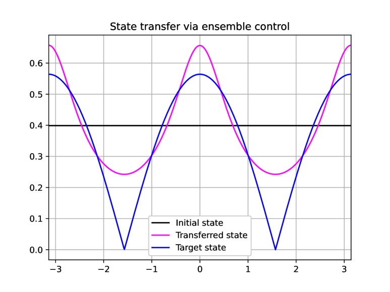
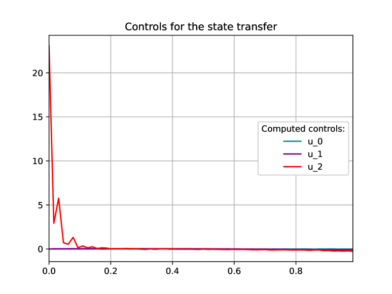
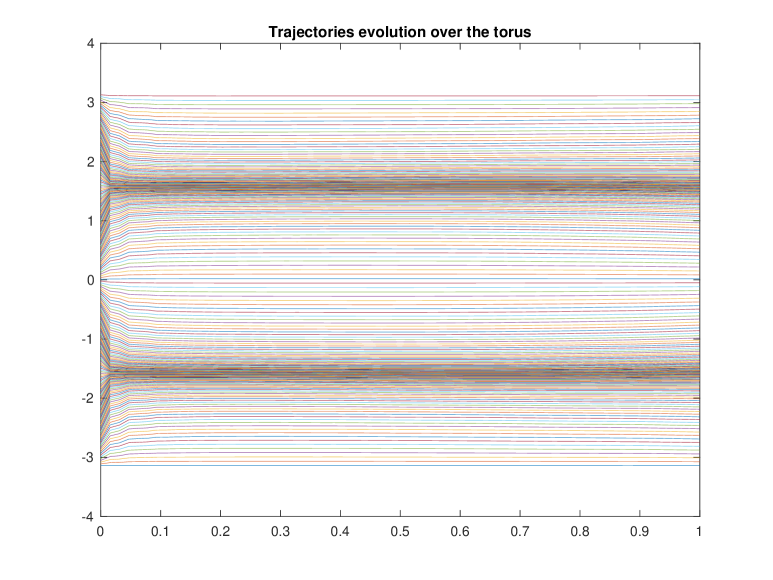
Figure 1. State transfer from the ground state $\psi_{0}\equiv\frac{1}{\sqrt{2\pi}}$ to the target state $\psi_{1}^{\prime}$ (see (4.3)). We used a random initialization for the control $u\in{\mathcal{U}}^{M}$, and we performed $1.5\cdot 10^{4}$ iterations of the gradient descent ($\sim 3$ mins of computational time). The resulting mismatch in the $L^{2}$-norm amounts at $0.2137$.

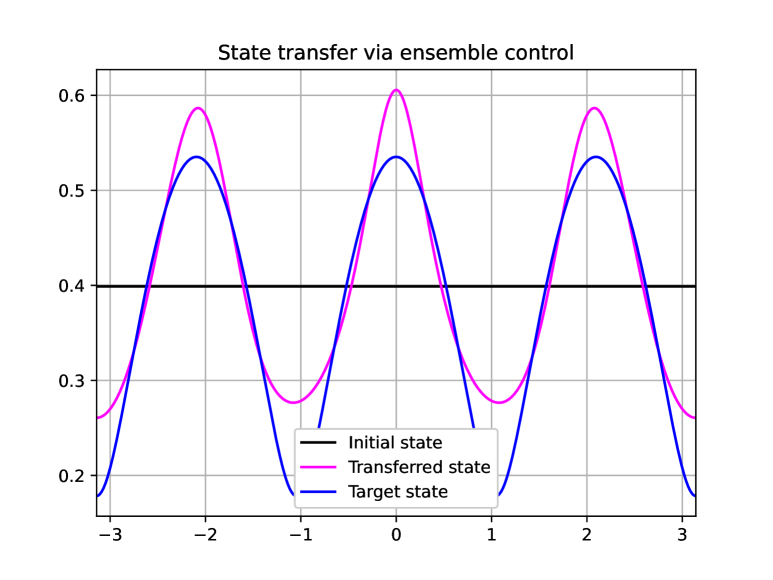
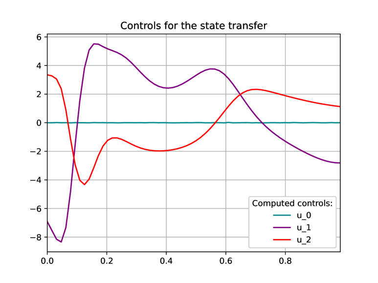
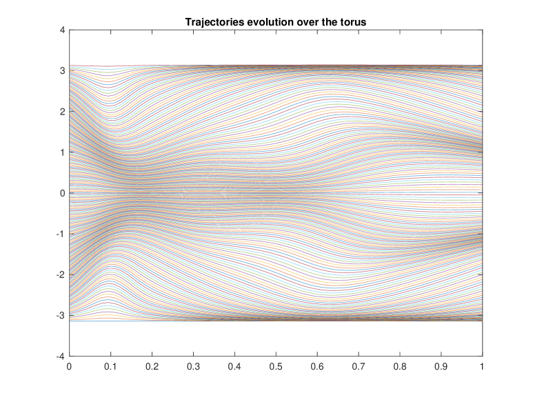
Figure 2. State transfer from the ground state $\psi_{0}\equiv\frac{1}{\sqrt{2\pi}}$ to the target state $\psi_{1}^{\prime\prime}$ (see (4.4)). We used a random initialization for the control $u\in{\mathcal{U}}^{M}$, and we performed $1.5\cdot 10^{4}$ iterations of the gradient descent ($\sim 3$ mins of computational time). The resulting mismatch in the $L^{2}$-norm amounts at $0.1098$.

Conclusions

In this paper, we proposed a method for constructing explicit control laws steering approximate state transfers in a bilinear Schrödinger PDE posed on the torus. Such systems are experimentally tested in physics and represent powerful platforms for quantum technology. Indeed, they model e.g. the orientational motion of rigid molecules, as well as the dynamics of cold atoms trapped in periodic optical lattices (known as Bose-Einstein condensates).

Even though small-time approximate controllability results have been recently established, determining explicitly such controls is, in general, challenging.

In the first part of the paper, we used geometric control arguments to rephrase the state transfer as a task of diffeomorphisms approximation. Then, relying on the powerful tools of $\Gamma$-convergence, we reduced the infinite-dimensional diffeomorphism approximation to a finite-ensemble control problem.

Finally, by taking advantage of this bridging, we performed some experiments and found explicit controls that achieve approximate state transfers numerically.

The errors in the state transfers are still significant (approximately $0.1$ and $0.2$), due to the highly nontrivial task of controlling simultaneously a large number of particles with vector fields that admit zeroes. The enhancement of these performances will be the subject of future investigation.

References

- [1] A. Agrachev and C. Letrouit. Generic controllability of equivariant systems and applications to particle systems and neural networks. Annales de l’Institut Henri Poincaré C, 2025.
- [2] A. Agrachev and A. Sarychev. Control on the manifolds of mappings with a view to the deep learning. Journal of Dynamical and Control Systems, 28(4):989–1008, 2022.
- [3] V. V. Albert, J. P. Covey, and J. Preskill. Robust encoding of a qubit in a molecule. Phys. Rev. X, 10:031050, Sep 2020.
- [4] K. Beauchard and E. Pozzoli. Small-time approximate controllability of bilinear Schrödinger equations and diffeomorphisms. 2025 arXiv:2410.02383v2.
- [5] K. Beauchard and E. Pozzoli. Examples of small-time controllable schrödinger equations. Annales Henri Poincaré, 2025.
- [6] U. Boscain, M. Caponigro, T. Chambrion, and M. Sigalotti. A weak spectral condition for the controllability of the bilinear Schrödinger equation with application to the control of a rotating planar molecule. Comm. Math. Phys., 311(2):423–455, 2012.
- [7] N. Boussaïd, M. Caponigro, and T. Chambrion. Small time reachable set of bilinear quantum systems. In 2012 IEEE 51st IEEE Conference on Decision and Control (CDC), pages 1083–1087, 2012.
- [8] A. Duca and V. Nersesyan. Bilinear control and growth of Sobolev norms for the nonlinear Schrödinger equation. Journal of the European Mathematical Society, 2023. in press.
- [9] N. Dupont, G. Chatelain, L. Gabardos, M. Arnal, J. Billy, B. Peaudecerf, D. Sugny, and D. Guéry-Odelin. Quantum state control of a bose-einstein condensate in an optical lattice. PRX Quantum, 2:040303, Oct 2021.
- [10] M. Fornasier, J. Klemenc, and A. Scagliotti. Trade-off invariance principle for minimizers of regularized functionals. arXiv preprint arXiv:2411.11639, 2024.
- [11] J. Glaser, T. Schulte-Herbrüggen, M. Sieveking, O. Schedletzky, N. Nielsen, O. Sørensen, and C. Griesinger. Unitary control in quantum ensembles: Maximizing signal intensity in coherent spectroscopy. Science, 280:421–424, 1998.
- [12] D. Gottesman, A. Kitaev, and J. Preskill. Encoding a qubit in an oscillator. Physical Review A, 64(1), Jun 2001.
- [13] R. Judson, K. Lehmann, H. Rabitz, and W. Warren. Optimal design of external fields for controlling molecular motion: application to rotation. Journal of Molecular Structure, 223:425 – 456, 1990.
- [14] N. Khaneja, R. Brockett, and S. J. Glaser. Time optimal control in spin systems. Physical Review A, 63(3), Feb 2001.
- [15] C. P. Koch, M. Lemeshko, and D. Sugny. Quantum control of molecular rotation. Rev. Mod. Phys., 91:035005, Sep 2019.
- [16] G. D. Maso. An Introduction to -convergence. Birkhäuser, ”Boston MA”, 1993.
- [17] P. Mason and M. Sigalotti. Generic controllability properties for the bilinear Schrödinger equation. Comm. Partial Differential Equations, 35(4):685–706, 2010.
- [18] J. Moser. On the volume elements on a manifold. Trans. Am. Math. Soc., 120:286–294, 1965.
- [19] S. Osnaghi, P. Bertet, A. Auffeves, P. Maioli, M. Brune, J. M. Raimond, and S. Haroche. Coherent control of an atomic collision in a cavity. Phys. Rev. Lett., 87:037902, Jun 2001.
- [20] M. Reed and B. Simon. Methods of Modern Mathematical Physics: I. Functional Analysis. Academic Press [Harcourt Brace Jovanovich, Publishers], New York-London, 1972.
- [21] M. Reed and B. Simon. Methods of modern mathematical physics. II. Fourier analysis, self-adjointness. Academic Press [Harcourt Brace Jovanovich, Publishers], New York-London, 1975.
- [22] A. Scagliotti. Deep learning approximation of diffeomorphisms via linear-control systems. Math. Control Relat. Fields, 13(3):1226–1257, 2023.
- [23] A. Scagliotti. Optimal control of ensembles of dynamical systems. ESAIM: Control Optim Calc. Var., 29, 2023.
- [24] A. Scagliotti. Minimax problems for ensembles of control-affine systems. SIAM J. Control Optim., 63(1):502–523, 2025.
- [25] A. Scagliotti and S. Farinelli. Normalizing flows as approximations of optimal transport maps via linear-control neural odes. arXiv preprint arXiv:2311.01404, 2023.
- [26] W. P. Thurston. Foliations and groups of diffeomorphisms. Bulletin of the American Mathematical Society, 80:304–307, 1974.