Transitions to Intermittent Chaos in Quorum Sensing Dynamics

Abstract

This study analyses the dynamical consequences of heterogeneous temporal delays within a quorum sensing-inspired (QS-inspired) system, specifically addressing the differential response kinetics of two subpopulations to signalling molecules. A nonlinear delay differential equation (DDE) model, predicated upon an activator-inhibitor framework, is formulated to represent the interspecies interactions. Key analytical techniques, including the derivation of the pseudo-characteristic polynomial and the determination of Hopf bifurcation criteria, are employed to investigate the stability properties of steady-state solutions. The analysis reveals the critical role of multiple, dissimilar delays in modulating system dynamics and inducing bifurcations. Numerical simulations, conducted in conjunction with analytical results, reveal the emergence of periodic self-sustained oscillations and intermittent chaotic behaviour. These observations emphasise the intricate relationship between temporal heterogeneity and the stability landscape of systems exhibiting QS-inspired dynamics. This interplay highlights the capacity for temporal variations to induce complex dynamical transitions within such systems. These findings assist to the comprehension of temporal dynamics within these and related systems, and may contribute to the development of strategies aimed at modulating intercellular communication and engineering synthetic biological systems with temporal control.

34C28, 34C23, 34H10, 37N25, 37D45

1 Introduction

Quorum sensing (QS) is a fundamental mechanism of microbial communication that was first proposed in the early 1970s to explain the bioluminescence observed in marine bacteria, particularly Vibrio fischeri [29]. Over the decades, QS has emerged as a sophisticated strategy that enables bacterial populations to synchronise their behaviour and enhance collective fitness. This process allows bacteria to assess their local density by monitoring the concentration of signalling molecules known as autoinducers. Once the concentration of autoinducers surpasses a critical threshold, a coordinated response is initiated, conferring advantages such as enhanced virulence [21, 23] and biofilm formation [17].

The study of QS mechanisms has been benefited from diverse mathematical modelling approaches, each offering unique insights into the underlying biological dynamics. These approaches span deterministic models, which describe average system behaviours; stochastic models, which account for intrinsic fluctuations; and hybrid models that combine both perspectives. For instance, Velázquez et al. [31] employed a continuous-time Markov process to investigate virulence in plant-pathogen interactions on leaf surfaces. Their model integrates linear birth rates, logistic death-migration processes, and an autocatalytic mechanism for acyl homoserine lactone autoinducers, revealing an inverse relationship between QS efficiency and the diffusion of autoinducers. Similarly, Frederick et al. [11] used a reaction-diffusion model with density-dependent diffusion coefficients to study extracellular polymeric substance (EPS) production in biofilms. They demonstrated how QS-regulated EPS production facilitates biofilms’ transition from a colonisation phase to a protective state, underscoring the adaptive benefits of QS in biofilm environments.

Delays and anomalous diffusion have also been key features in deterministic modelling approaches. Kuttler et al. [19] explored anomalous diffusion processes to model delayed substance transport caused by transcriptional delays. Chen et al. [5], Elowitz et al. [7], and Ojalvo et al. [12] studied QS pathways using gene regulatory networks with feedforward and negative feedback loops. Their models incorporated transcriptional time delays to explore phenomena such as Hopf bifurcations and sustained oscillations. These studies showed that transcriptional delays can act as critical parameters, leading to oscillatory and complex behaviours, particularly in the context of QS-regulated drug delivery systems for cancer therapy.

In bacterial QS, specialised receptor proteins detect autoinducers, triggering gene expression changes that orchestrate collective behaviours. These changes lead to a division into two sub-populations: motile (up-regulated), which engage in collective activities, and static (down-regulated), which remain inactive. However, transitions between these states are not instantaneous, as biochemical processes like transcription and translation introduce inherent time delays [22, 27, 38, 37]. These delays, which reflect processes such as signal production, diffusion, and cellular response, significantly influence the timing and robustness of QS-driven behaviours [28].

The inclusion of time delays in QS models is crucial for accurately capturing the temporal dynamics of bacterial communication. For example, Barbarossa et al. [1] developed a delay differential equations (DDE) model for Pseudomonas putida to explain experimental observations of autoinducer production. Their results supported the hypothesis of an enzyme degrading autoinducers into an inactive form, thereby introducing a feedback delay. Time delays have been shown to induce oscillatory behaviours, as demonstrated in [4, 3], where the amplitude and frequency of oscillations depended on the delay length. Furthermore, bifurcation analyses of QS models have revealed transitions between stable steady states, periodic oscillations, chaotic behaviours (e.g. [24, 16, 18]), and multi-stability [35]. These features align with experimental observations where bacterial populations exhibit synchronised or desynchronised behaviours under varying environmental conditions [14].

Incorporating these temporal factors into QS models not only enriches our understanding of microbial communication but also strengthen the development of practical applications. Manipulating QS systems can lead to novel strategies for microbial control and synthetic biology, with potential implications for environmental management and medical therapeutics [9, 10, 39, 40]. For instance, in [4], a single delay introduced into a QS model led to sustained oscillations in signalling molecule concentrations, highlighting the pivotal role of temporal factors in QS regulation. Moreover, Chen et al. [5] analysed the effects of two distinct delays: one representing the time required for autoinducers to diffuse and another capturing the lag between signal detection and target gene expression. Their results demonstrated the importance of these delays in driving oscillatory behaviours and determining system stability.

In the present manuscript, we analyse a nonlinear DDE quorum sensing system in which motile and static bacterial sub-populations respond differently to autoinducers due to distinct response times. This is characterised by the introduction of two independent delay parameters, $\tau_{1}>0$ and $\tau_{2}>0$, corresponding to the motile and static sub-populations, respectively. A local stability analysis is conducted by varying these delay parameters, identifying diverse bifurcations and the conditions under which they arise. These findings contribute to a deeper understanding of how time delays shape the dynamics of QS systems, particularly in the context of bifurcations and stability transitions.

The manuscript is structured as follows: Section 2 introduces the nonlinear time-delayed QS system under investigation, detailing the model’s assumptions and highlighting the activator-inhibitor framework employed to represent the dynamic interplay between motile and static bacterial subpopulations. Section 3 rigorously analyzes the existence and local stability properties of the system’s steady states, deriving the pseudo-characteristic polynomial and formulating conditions for the emergence of purely imaginary eigenvalues, thereby facilitating the analysis of Hopf bifurcations. Section 4 presents the results of extensive numerical simulations, exploring the system’s dynamical behavior across a range of parameter values and illustrating the profound influence of varying delay parameters on the system’s dynamics. A detailed analysis of the observed intermittent chaotic behaviour, including a discussion of its characteristics and underlying mechanisms, is presented in Section 5. Finally, Section 6 concludes the manuscript with a comprehensive discussion of the key findings, emphasising their implications for advancing our understanding of QS-inspired systems and, in particular, the emergence of complex dynamical behaviour in the presence of multiple delays.

2 Nonlinear time delayed Quorum Sensing system

The present work investigates the dynamics of QS, emphasising the critical role of local interactions mediated by autoinducer concentrations. Autoinducers are signalling molecules produced by both motile and static bacteria, following the law of mass action, whose production rates increase with bacterial population density. The growth of motile bacteria is intrinsically driven as well as is inhibited by the presence of static bacteria, with long-term behaviour regulated by environmental saturation constraints.

The bacterial population dynamics in this context can be modelled using an activator-inhibitor framework analogous to the Gierer–Meinhardt system. Here, motile bacteria function as activators, driving QS processes, while static bacteria act as inhibitors, imposing regulatory constraints. To reduce the complexity of the parameter space and address scenarios where static bacteria may be negligible, rescaling transformations and desingularisation techniques are employed. The resulting QS model is governed by the following system of equations, as described in [18]:

(1a) $$\dot{w} =dv(u+v)-cwv,$$

(1b) $$\dot{v} =wvu^{2}+a\varepsilon v-v^{2},$$

(1c) $$\dot{u} =\frac{wu^{2}}{1+Ku^{2}}+av-buv,$$

where $w$, $v$, and $u$ represent the concentrations of autoinducers, static bacteria, and motile bacteria subpopulations, respectively. The parameters are defined as follows: (i) $K$is the saturation parameter, modulating the regulatory effects of autoinducer concentrations, (ii) $a$and $\varepsilon a$ denote the production rates of autoinducers and the bacterial population, respectively, (iii) $b$is the decay rate of the bacterial population, and (iv) $c$and $d$ describe the decay and production rates of autoinducers.

The system in (1) encompasses the dynamic interplay between motile and static bacteria populations, governed by their interactions with autoinducers. Specifically: (i) the rate of change of the autoinducer concentration depends on the production and decay rates driven by interactions between motile and static bacteria; (ii) the static bacteria concentration evolves according to its interactions with autoinducers and its own production-decay dynamics; (iii) the motile bacteria concentration is influenced by its interactions with autoinducers and static bacteria, along with intrinsic production and decay rates.

This study advances a rigorous framework, predicated upon an activator-inhibitor paradigm, for the comprehensive analysis of QS regulatory mechanisms and localised interaction dynamics. By explicitly formulating the dependence of bacterial population dynamics on cell densities and autoinducer-mediated feedback loops, the framework captures the salient features of QS behaviour. Notably, the application of rescaling transformations enhances the model’s applicability, particularly in scenarios characterised by the absence of static bacterial populations.

Beyond its methodological contributions, this work provides novel insights into the nuanced dynamics of microbial communication within spatially constrained environments. The model elucidates the synergistic interplay between localised interactions and intrinsic regulatory mechanisms in shaping emergent bacterial population dynamics, offering critical perspectives on the complex, density-dependent behaviours characteristic of QS systems. These findings establish a robust theoretical foundation for the systematic investigation of QS dynamics across diverse environmental and biological contexts, facilitating advancements in fields such as microbial ecology, systems biology, and biomedical engineering. Specifically, the rescaling transformations further enhance the model’s applicability, particularly in cases where static bacteria may be absent.

$a$	$b$	$\varepsilon$	$c$	$d$	$K$	$\tau_{1}$	$\tau_{2}$
$0.0428$	$[1.2,1.5]$	$0.1$	$0.16$	$0.0522$	$0.0435$	$[0,500]$	$[0,500]$

Table 1: Parameter values set.

As the bacterial response to stimuli communicated by autoinducers is not necessarily instantaneous, it is reasonable to hypothesise that this response may depend on intrinsic receptor properties within each sub-population or on bacterial activities carried out at earlier times.

To account for these temporal effects, the original system (1) is extended by incorporating delayed autoinducer concentrations into the growth rates. Specifically, let $w_{1}=w(t-\tau_{1})$ and $w_{2}=w(t-\tau_{2})$, where $\tau_{1}>0$ and $\tau_{2}>0$ represent the delay times associated with the non-instantaneous responses of motile and static bacteria, respectively. The modified QS system is then given by:

(2a) $$\dot{w} =dv(u+v)-cwv,$$

(2b) $$\dot{v} =w_{1}vu^{2}+a\varepsilon v-v^{2},$$

(2c) $$\dot{u} =\frac{w_{2}u^{2}}{1+Ku^{2}}+av-buv,$$

where the parameters retain their original definitions, as described earlier, and their distinguished values are as in Table 1.

Notice that the inclusion of delays $\tau_{1}$ and $\tau_{2}$ introduces additional complexity to the system dynamics, as these delays reflect the temporal lag between autoinducer production and its regulatory effects on bacterial populations. The delayed terms $w_{1}$ and $w_{2}$ capture the influence of past autoinducer concentrations on the current growth rates of static and motile bacteria, respectively. Our analysis focuses on examining the dynamic impact of these delays, particularly how they influence stability and potential bifurcation phenomena.

3 Steady-states and local stability.

To initiate our analysis, we first establish the existence and positivity of steady-states under the parameter values specified in Table 1. Subsequently, we proceed to examine the local stability properties of these steady-states to gain insights into the system’s dynamic behaviour.

3.1 Positive steady-states.

Biologically meaningful steady-states of system (2) correspond to constant solutions that lie within the first octant. These steady-states can be determined by solving the following algebraic system:

(3a) $$\left[(u+v)d-cw\right]v=0\,,$$

(3b) $$\left(wu^{2}+a\varepsilon-v\right)v=0\,,$$

(3c) $$wu^{2}+\left(a-bu\right)\left(1+Ku^{2}\right)v=0\,,$$

where $w_{1}=w_{2}=w$, since steady-states are temporally invariant.

The null steady-state $(w,v,u)=(0,0,0)$ corresponds to the absence of bacterial populations and autoinducer concentration. For non-trivial steady-states, equation (3a) provides the following expression for $w$:

(4a) $$w=\frac{d(u+v)}{c}>0\,,$$

which can be substituted into (3b), yielding the expression for $$v$$:

(4b) $$v=\frac{du^{3}+a\varepsilon c}{c-du^{2}}\,,$$

provided that $|u|<\sqrt{c/d}$ is satisfied to ensure $v>0$. Substituting (4a) and (4b) into (3c) reduces the system to solving $f_{eq}(u)=0$, where $f_{eq}(u)$ is a monic polynomial of degree six, given by

(5) $$f_{eq}(u):= \>u^{6}-\frac{a}{b}u^{5}+\frac{1}{K}u^{4}-\frac{ad+d-ba\varepsilon cK}{bdK}u^{3}$$

$$-\frac{da\varepsilon+a^{2}\varepsilon cK}{bdK}u^{2}+\frac{a\varepsilon c}{dK}u-\frac{a^{2}\varepsilon c}{bdK}\,.$$

Since all coefficients of $f_{eq}(u)$ are real, the Fundamental Theorem of Algebra guarantees six roots in total, which may include real and complex ones. The number of positive, negative, and complex roots is constrained by Descartes’ rule of signs. That is, based on the five sign changes in the polynomial’s coefficients, provided $(a+1)d>ba\varepsilon cK$, three possible configurations arise: (i) five positive roots and one negative root; (ii) three positive roots, one negative root, and two complex conjugate roots; (iii) one positive root, one negative root, and four complex conjugate roots.

To refine this further, the Sturm Theorem [36] can be applied to determine the number of distinct real roots of (5) within the interval $|u|<\sqrt{c/d}$. Specifically, the difference in sign variations of the Sturm sequence at the interval’s endpoints provides the number of real roots in the interval. Using the parameter values given in Table 1 with $b=1.4$, the signs of the Sturm sequence are calculated at the ends of the interval of consideration as follows: (a) at $u=-1.75$, the sequence is $$S(-1.75)=\{+,-,-,+,-,+,-\}$$ , resulting in $V(-1.75)=5$ sign changes; (b) at $u=1.75$, the sequence is $$S(1.75)=\{+,+,-,-,-,-,-\}$$ , resulting in $V(1.75)=1$ sign change. Hence, the number of real roots within the interval is given by $V(-1.75)-V(1.75)=4$. Combining this result with Descartes’ rule of signs confirms that the roots of $f_{eq}(u)$ comprise three positive, one negative, and two complex conjugate roots. In consequence, there are three steady-states lying within the first octant.

3.2 Time delayed QS local stability.

Now, to analyse the local stability properties of the system, let us denote the positive steady-states as $E_{1},E_{2},E_{3}\in\mathbb{R}^{3}$. The pseudo-characteristic polynomial at these steady-states is given by (see, for instance, [26]):

(6a) $$\det(\mathbf{J}_{0}+\exp(-\lambda\tau_{1})\mathbf{J}_{\tau_{1}}+\exp(-\lambda\tau_{2})\mathbf{J}_{\tau_{2}}-\lambda\mathbf{I}_{3\times 3})=0\,,$$

where $$\mathbf{I}_{3\times 3} \mathbf{J}_{0} \mathbf{J}_{\tau_{1}} \mathbf{J}_{\tau_{2}}$$ is the identity matrix, and the matrices , , and are defined as follows:

(6b) $$\mathbf{J}_{0}=\begin{pmatrix}-cv&du+2dv-cw&dv\\ 0&w_{1}u^{2}+a\varepsilon-2v&2w_{1}vu\\ 0&a-bu&\frac{2uw_{2}}{(1+Ku^{2})^{2}}-bv\end{pmatrix}\,,$$

(6c) $$\mathbf{J}_{\tau_{1}}=\begin{pmatrix}0&0&0\\ vu^{2}&0&0\\ 0&0&0\end{pmatrix}\,,\quad\mathbf{J}_{\tau_{2}}=\begin{pmatrix}0&0&0\\ 0&0&0\\ \frac{u^{2}}{1+Ku^{2}}&0&0\end{pmatrix}\,.$$

The matrix $\mathbf{J}_{0}$ corresponds to the Jacobian evaluated at the steady-state in the absence of delays, while $\mathbf{J}_{\tau_{1}}$ and $\mathbf{J}_{\tau_{2}}$ capture the contributions from delayed interactions associated with $w_{1}=w(t-\tau_{1})$ and $w_{2}=w(t-\tau_{2})$, respectively. These delay terms reflect the biological reality that bacterial responses to autoinducers may not be instantaneous, depending on the activity of each subpopulation or autoinducers response characteristics.

The determinant condition in (6) incorporates the interplay of delays in the system’s dynamics, where the $\tau_{1,2}$-dependent exponential terms introduce non-trivial dependencies on the delay parameters. These factors fundamentally affect the stability of the steady-states, as they influence the eigenvalue spectrum of the pseudo-characteristic equation.

Notice that the structure of the matrices $\mathbf{J}_{0}$, $\mathbf{J}_{\tau_{1}}$, and $\mathbf{J}_{\tau_{2}}$ highlights the coupling between up- and down-regulated bacteria, and autoinducer concentrations. In other words, (i) the matrix (6b) encapsulates the direct interactions and self-regulation of each variable; (ii) the left-hand side delay matrix in (6c) accounts for the delayed contribution of motile bacteria to the growth of static bacteria via autoinducer-mediated interactions; (iii) similarly, right-hand side delay matrix in (6c) reflects the delayed influence of motile bacteria on their own growth due to the saturation effects regulated by autoinducer concentration.

As the pseudo-characteristic polynomial (6) defines a transcendental equation, it inherently possesses an infinite number of roots due to the presence of exponential terms. These roots, corresponding to the eigenvalues of the linearised system, determine the growth rates and oscillatory behaviours of the dynamics. However, such linearisation at any steady-state is characterised by at most a finite number of eigenvalues with positive real parts, which correspond to unstable modes. The remaining eigenvalues typically have negative real parts or tend asymptotically to $-\infty$. As a consequence, despite the infinite-dimensional nature of system (2), which arises from their dependence on the history of the solution over the delays interval, bifurcation theory reveals that their nonlinear dynamical events are qualitatively analogous to those of ordinary differential equations; see, for instance, [20, 2].

Observe that the determinant in (6) gives rise to the quasi-polynomial expression

(7a) $$q(\lambda,\boldsymbol{\tau},\mathbf{p})= \>p_{3}(\lambda,\mathbf{p})+p_{2}(\lambda,\mathbf{p})\exp(-\lambda\tau_{2})+p_{1}(\lambda,\mathbf{p})\exp(-\lambda\tau_{1})\,,$$

where

$$p_{3}(\lambda,\boldsymbol{\tau},\mathbf{p})= \>(-cv-\lambda)\bigg{[}\big{(}a\varepsilon-\lambda+u^{2}{w_{1}}-2v\big{)}\bigg{(}-bv-\lambda+\frac{2u{w_{2}}}{\big{(}Ku^{2}+1\big{)}^{2}}\bigg{)}$$

(7b) $$\quad-2uv{w_{1}}(a-bu)\bigg{]}\,,$$

(7c) $$p_{2}(\lambda,\boldsymbol{\tau},\mathbf{p})= \>\frac{u^{2}v}{Ku^{2}+1}\big{(}-ad\varepsilon-2cuw{w_{1}}-du^{2}{w_{1}}+4duv{w_{1}}+2dv+d\lambda\big{)},$$

$$p_{1}(\lambda,\boldsymbol{\tau},\mathbf{p})= \>-u^{2}v(-cw+du+2dv)\bigg{(}-bv-\lambda+\frac{2u{w_{2}}}{\big{(}Ku^{2}+1\big{)}^{2}}\bigg{)}$$

(7d) $$\quad+du^{2}v^{2}(a-bu)\,;$$

here, $\boldsymbol{\tau}=(\tau_{1},\tau_{2})^{T}$ represents the delay vector, while $\mathbf{p}=(a,b,c,d,\varepsilon,K)^{T}$ encapsulates the system parameter vector.

3.2.1 Existence of purely imaginary eigenvalues.

We begin our analysis by considering the non-delayed case in (7a). In so doing, it is reduced to the polynomial determined by (7) with $\tau_{1}=\tau_{2}=0$. For the parameter values given in Table 1, the positive steady-states $E_{1}$, $E_{2}$, and $E_{3}$ correspond to hyperbolic points. Specifically, $E_{2}$ is a saddle point, while $E_{3}$ corresponds to a stable node. In particular, the steady-state $E_{1}$ exhibits a saddle-type instability as is characterised by the presence of one real negative eigenvalue and a pair of complex conjugate eigenvalues with positive real parts. Furthermore, the number of positive steady-states and their corresponding stability properties align precisely with the results reported in [18], which states the robustness and validity of our theoretical framework.

For sufficiently small positive values of the delays, $0<\tau_{1},\tau_{2}\ll 1$, the number of eigenvalues $\lambda$ satisfying $q(\lambda,\boldsymbol{\tau},\mathbf{p})=0$ not only becomes infinite, but also the real parts of these eigenvalues drift: they shift to the right when $\Re{(\lambda)}$ is negative and to the left when $\Re{(\lambda)}$ is positive. This phenomenon suggests a transition in stability, which is intrinsically linked to the emergence of purely imaginary eigenvalues; see, for a detailed discussion, [26].

To determine purely imaginary roots of (7a), let us set $\lambda=i\omega$ for $\omega>0$, yielding

(8) $$p_{3}(i\omega,\mathbf{p})+p_{2}(i\omega,\mathbf{p})e^{-i\omega\tau_{2}}+p_{1}(i\omega,\mathbf{p})e^{-i\omega\tau_{1}}=0\,.$$

First, observe that (7b) has no zeros on the imaginary axis at the steady-states $E_{1},E_{2},E_{3}$ for the parameter values given in Table 1. Consequently, defining $q_{i}(i\omega)=p_{i}(i\omega,\mathbf{p})/p_{3}(i\omega,\mathbf{p})$ for $i=1,2$, where we have omitted explicit dependence on $\mathbf{p}$ to ease notation, the pseudo-polynomial in (8) can be rewritten as

(9a) $$1+q_{1}(i\omega)e^{-i\omega\tau_{1}}+q_{2}(i\omega)e^{-i\omega\tau_{2}}=0\,,$$

which leads to $$|q_{1}(i\omega)e^{-i\omega\tau_{1}}+q_{2}(i\omega)e^{-i\omega\tau_{2}}|=1 A(\omega)=\operatorname{Re}(\overline{q_{1}(i\omega)}q_{2}(i\omega)) B(\omega)=-\operatorname{Im}(\overline{q_{1}(i\omega)}q_{2}(i\omega)) h=\tau_{1}-\tau_{2}$$. Notice that, upon introducing the definitions , and , it can be recasted as

(9b) $$|q_{1}(i\omega)|^{2}+|q_{2}(i\omega)|^{2}+2R(\omega)\cos(\omega h-\alpha(\omega))=1\,,$$

where $R(\omega)=\sqrt{A^{2}(\omega)+B^{2}(\omega)}$ and $\tan\alpha(\omega)=B(\omega)/A(\omega)$.

From equation (9b), the existence of roots of $q(i\omega,\boldsymbol{\tau},\mathbf{p})$ is ensured if the following conditions hold uniquely and simultaneously:

(10a) $$\left|1-|q_{1}(i\omega)|^{2}-|q_{2}(i\omega)|^{2}\right|\leq 2R(\omega)\,,$$

(10b) $$\xi(\omega)=\cos(\omega h-\alpha(\omega))\,,$$

where

$$\xi(\omega)=\frac{1-|q_{1}(i\omega)|^{2}-|q_{2}(i\omega)|^{2}}{2R(\omega)}\,.$$

Condition (10a) ensures that $|\xi(\omega)|\leq 1$, which constitutes a necessary criterion for the solvability of equation (10b). Consequently, the roots of (8) correspond to values of $h\in\mathbb{R}$ and $\omega>0$ at which the functions $\xi(\omega)$ and $\cos(\omega h-\alpha(\omega))$ intersect. This behaviour is depicted in Figure 1(a), which illustrates the intersection points for the steady-state $E_{1}$ at three distinct values of $h$. A similar pattern is observed for the steady-state $E_{2}$, as is shown in Figure 1(b). Notably, the orders of magnitude of $h$ at which these intersections occur differ significantly between the two steady-states: for $E_{1}$, intersections arise at values of $h$ on the order of $10^{2}$, whereas for $E_{2}$, they occur at values two orders of magnitude greater. In both cases, the frequency of oscillations in $\cos(\omega h-\alpha(\omega))$ increases proportionally with $h$, facilitating the number of intersections, which suggests that the emergence of purely imaginary roots is strongly influenced by the introduction of two distinct delay terms, particularly when their magnitudes differ considerably. On the other hand, the steady-state $E_{3}$ is evaluated in the functions $\xi(\omega)$ and $\cos(\cdot)$. In this case, it is disclosed that $|\xi(\omega)|>1$ for all $\omega\geq 0$. Consequently, condition (10a) is hence not satisfied, preventing the existence of intersection solutions for (10b), which results in confirming that $E_{3}$ remains stable for all $\tau_{1},\tau_{2}>0$.

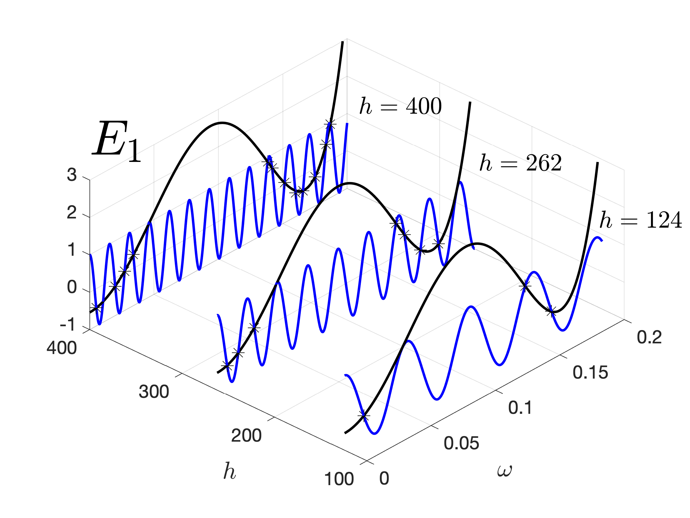
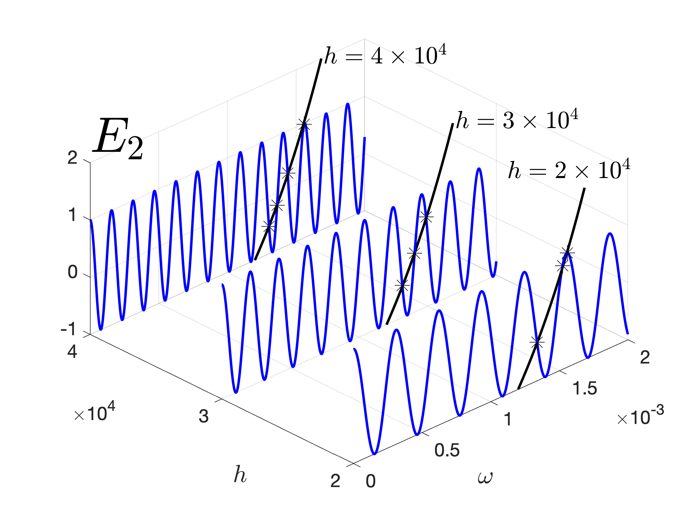
$(a)$                   $(b)$

Figure 1: Graphs of $\xi(\omega)$ (black) and $\cos(\cdot)$ (blue), along with their intersection points, are shown for the steady-states: (a) $E_{1}$ at $h=124,262,400$; (b) $E_{2}$ at $h=2\times 10^{4},3\times 10^{4},4\times 10^{4}$. All other parameter values are as in Table 1.

3.2.2 A geometric transversality condition.

Once we have established the existence of imaginary roots for the pseudo-polynomial (7), we now provide a geometric characterisation of their crossing of the imaginary axis as a function of the delays $\tau_{1},\tau_{2}>0$. Given the oscillatory behaviour of the steady-state $E_{1}$ at $\tau_{1}=\tau_{2}=0$, our analysis is focused on this point. Crucially, $q(0,\boldsymbol{\tau},\mathbf{p})\neq 0$, as shown by (7). Furthermore, the polynomials $p_{i}(\lambda,\boldsymbol{\tau},\mathbf{p})$, for $i=1,2,3$, defined in (7b)-(7d), are numerically verified to have no common zeros, and $\deg(p_{3}(\lambda,\boldsymbol{\tau},\mathbf{p}))>\max\{\deg(p_{2}(\lambda,\boldsymbol{\tau},\mathbf{p})),\deg(p_{1}(\lambda,\boldsymbol{\tau},\mathbf{p}))\}$. These conditions ensure that for $E_{1}$, there exist values of $\tau_{1}$ and $\tau_{2}$ for which the real parts of the roots of $q(\lambda,\boldsymbol{\tau},\mathbf{p})$ lie in the left-hand side of the complex plane; see, for instance, [15].

To characterise the intersections, we interpret the three terms in (9a) as vectors in the complex plane. The first term has a magnitude of unity and is oriented along the real axis. The remaining two terms are given by $|q_{j}(i\omega)|\exp(-i\omega\tau_{j}+i\arg(q_{j}(i\omega)))$, for $j=1,2$. Since equation (9a) holds, these vector orientations must form a triangle. This geometric constraint is satisfied only for non-zero values of $\omega$ that also fulfill the conditions stated in Proposition 3.1 of [15]:

(11) $$1\leq\left|q_{1}(i\omega)\right|+\left|q_{2}(i\omega)\right|\,,\quad-1\leq\left|q_{1}(i\omega)\right|-\left|q_{2}(i\omega)\right|\leq 1\,.$$

These conditions are illustrated in Figure 2(a) at the steady-state $E_{1}$. As is depicted there, inequalities in (11) are simultaneously satisfied only within the subintervals $\Omega_{1}=[0,0.0466554]$ and $\Omega_{2}=[0.136335,0.187117]$ for the parameter values given in Table 1.

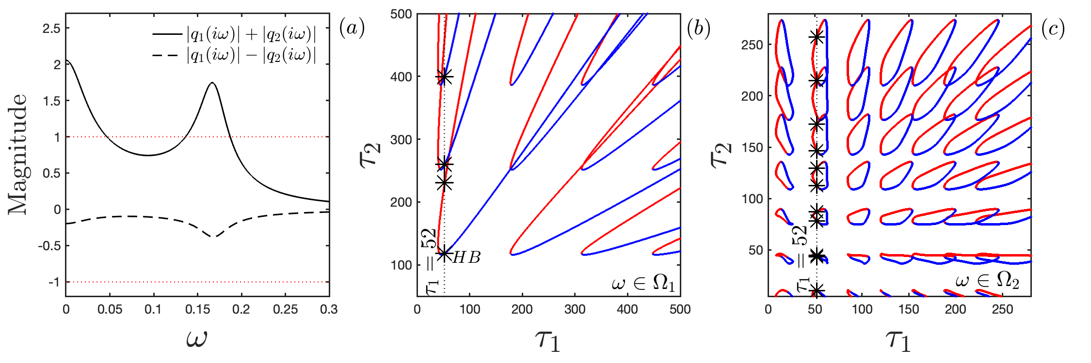
Figure 2: Purely imaginary eigenvalues for $\tau_{1},\tau_{2}>0$ for low and high frequency intervals. (a) Conditions in (11) hold for $\omega>0$ within the two distinct frequency intervals given by $\Omega_{1}=[0,0.0466554]$ and $\Omega_{2}=[0.136335,0.187117]$. (b)-(c) Sets of positive delay values for which the pseudo-polynomial (7) admits at least one zero of the form $\lambda=i\omega$ with $\omega\in\Omega_{1}=[0,0.0466554]$ (panel (b)) and $\omega\in\Omega_{2}=[0.136335,0.187117]$ (panel (c)). The asterisks mark points in (b) and (c) correspond to the specific case of $\tau_{1}=52$. Delay values satisfying the transversality parameter (13) to be positive are in red, otherwise correspond to blue solid curves. Other parameter values as in Table 1.

Now, as is established in [15], equation (9a) yields expressions for the delays, $\tau_{1}=\tau_{1}^{n\pm}(\omega)$ and $\tau_{2}=\tau_{2}^{m\pm}(\omega)$, as functions of $\omega>0$, given by

(12a) $$\tau_{1}^{n^{\pm}}(\omega)=\frac{\arg(q_{1}(i\omega))}{\omega}\pm\frac{1}{\omega}\arccos\left(\frac{1+|q_{1}(i\omega)|^{2}-|q_{2}(i\omega)|^{2}}{2|q_{1}(i\omega)|}\right)+\frac{(2n-1)\pi}{\omega},$$

(12b) $$\tau_{2}^{m^{\pm}}(\omega)=\frac{\arg(q_{2}(i\omega))}{\omega}\mp\frac{1}{\omega}\arccos\left(\frac{1+|q_{2}(i\omega)|^{2}-|q_{1}(i\omega)|^{2}}{2|q_{2}(i\omega)|}\right)+\frac{(2m-1)\pi}{\omega},$$

where $n$ and $m$ are integers such that $n=n_{0}^{+},n_{0}^{+}+1,n_{0}^{+}+2,\dots$ and $m=m_{0}^{+},m_{0}^{+}+1,m_{0}^{+}+2,\dots$, respectively. Here, $n_{0}^{+}$, $n_{0}^{-}$, $m_{0}^{+}$, and $m_{0}^{-}$ represent the smallest non negative integers for which $\tau_{1}^{n_{0}^{\pm}}$ and $\tau_{2}^{m_{0}^{\pm}}$ are non negative. These delay values can be gathered in the set $\mathcal{T}_{\omega,n,m}^{\pm}=\left\{(\tau_{1}^{n^{\pm}}(\omega),\tau_{2}^{m^{\pm}}(\omega))\right\}\subset\mathbb{R}_{+}^{2}$, parameterised by $\omega>0$, and define $\mathcal{T}_{n,m}^{\pm k}=\bigcup_{\omega\in\Omega_{k}}\mathcal{T}_{\omega,n,m}^{\pm}$ for $k=1,2$. Hence, the set $\mathcal{T}=\mathcal{T}^{1}\cup\mathcal{T}^{2}$, where

$$\mathcal{T}^{k}=\bigcup_{n,m\in\mathbb{Z}}\left(\mathcal{T}_{n,m}^{+k}\cup\mathcal{T}_{n,m}^{-k}\right)\cap\mathbb{R}_{+}^{2}\,,\quad k=1,2\,,$$

consists of all points $(\tau_{1},\tau_{2})\in\mathbb{R}_{+}^{2}$ for which the pseudo-polynomial $q(i\omega,\boldsymbol{\tau},\mathbf{p})$ possesses at least one zero on the imaginary axis; see [15]. In Figure 2, the points $(\tau_{1},\tau_{2})$ in the $\mathbb{R}_{+}^{2}$ plane corresponding to the sets $\mathcal{T}^{1}$, for $\omega\in\Omega_{1}$, and $\mathcal{T}^{2}$, for $\omega\in\Omega_{2}$, can be seen in panels (b) and (c), respectively, for the parameter set values in Table 1.

To analyse the direction of imaginary axis crossings for the roots of $q(\lambda,\boldsymbol{\tau},\mathbf{p})$ at points $(\tau_{1},\tau_{2})\in\mathcal{T}^{k}$, where $k=1,2$, we consider eigenvalues of the form $\lambda=\sigma+i\omega$. Specifically, we examine how the real part, $\sigma$, changes as the delays vary.

First, we define the tangent vector to $\mathcal{T}^{k}$ along the curve of increasing $\omega$ as $\mathbf{w}_{\theta}=(\partial\tau_{1}/\partial\omega,\partial\tau_{2}/\partial\omega)$. A normal vector pointing towards the left-hand region of the positively oriented curve $\mathcal{T}^{k}$ is then provided by $\mathbf{v}_{\theta}=(-\partial\tau_{2}/\partial\omega,\partial\tau_{1}/\partial\omega)$.

Second, we consider the scenario where a pair of complex conjugate roots of $q(\lambda,\boldsymbol{\tau},\mathbf{p})$ crosses the imaginary axis into the right-hand side of the complex plane. In this case, the delay vector $\boldsymbol{\tau}=(\tau_{1},\tau_{2})$ shifts parallel to the vector $\mathbf{w}_{r}=(\partial\tau_{1}/\partial\sigma,\partial\tau_{2}/\partial\sigma)$. Consequently, if $\boldsymbol{\tau}\in\mathbb{R}_{+}^{2}$ lies to the left of a positively oriented trajectory $\mathcal{T}^{k}$, two additional roots of $q(\lambda,\boldsymbol{\tau},\mathbf{p})$ become unstable when the inner product $\langle\mathbf{w}_{r}\,,\mathbf{v}_{\theta}\rangle>0$. Thus, as a consequence of the Implicit Function Theorem and Proposition 6.1 of [15], this condition is equivalent to $\mathcal{C}>0$, where

(13) $$\mathcal{C}:=\text{Im}\left(q_{1}(i\omega)q_{2}(-i\omega)e^{i\omega(\tau_{2}-\tau_{1})}\right)\,,$$

which is known as geometric transversality parameter as it provides a criterion for determining the crossing direction of the roots.

The parameter $\mathcal{C}$, defined in (13), characterises the direction of root crossing and, consequently, the type of Hopf bifurcation. Figure 2(b)-(c) visualises the delays $(\tau_{1},\tau_{2})$ categorised by this parameter. Red curves delineate regions where $\mathcal{C}<0$, while blue regions represent $\mathcal{C}>0$. Each intersection of a root of $q(\lambda,\boldsymbol{\tau},\mathbf{p})$ with the imaginary axis corresponds to a Hopf bifurcation. Specifically, a supercritical Hopf bifurcation occurs when the root crosses from left to right (i.e., $\mathcal{C}>0$), while a subcritical Hopf bifurcation occurs for a crossing from right to left (i.e., $\mathcal{C}<0$). The likelihood of these bifurcations increases with the difference between the delays, $|\tau_{1}-\tau_{2}|$. Moreover, the direction of root crossing exhibits a quasi-periodic behaviour, as illustrated in Figure 2(b)-(c). These results further suggest a dependence of the bifurcation type on the frequency. Specifically, the emergence of $\alpha$- and $\omega$-limit cycles is observed across a range of oscillatory frequencies. These limit cycles manifest at both lower frequencies (Figure 2(b)) and elevated frequencies (Figure 2(c)), a phenomenon associated with an alternating sequence of criticality transitions. This observation underscores the nuanced relationship between oscillatory dynamics and system criticality within the explored parameter set values.

4 Numerical bifurcation analysis of time delay QS system.

As established in the preceding section, the introduction of two delays significantly alters the system’s dynamics, inducing self-sustained oscillations through Hopf bifurcations. To further investigate this phenomenon, we fix the time delay $\tau_{1}$ at a specific value and slowly vary $\tau_{2}$. The resulting bifurcation diagram is shown in Figure 3, where their dynamical behaviour is initially depicted in Figure 2(b) and 2(c), where a countably infinite set of $\tau_{2}$ values at which Hopf bifurcations occur can be seen. This is illustrated by the distribution of asterisks along the dotted line $\tau_{1}=52$ in Figure 2(b) and 2(c), each marking a bifurcation point.

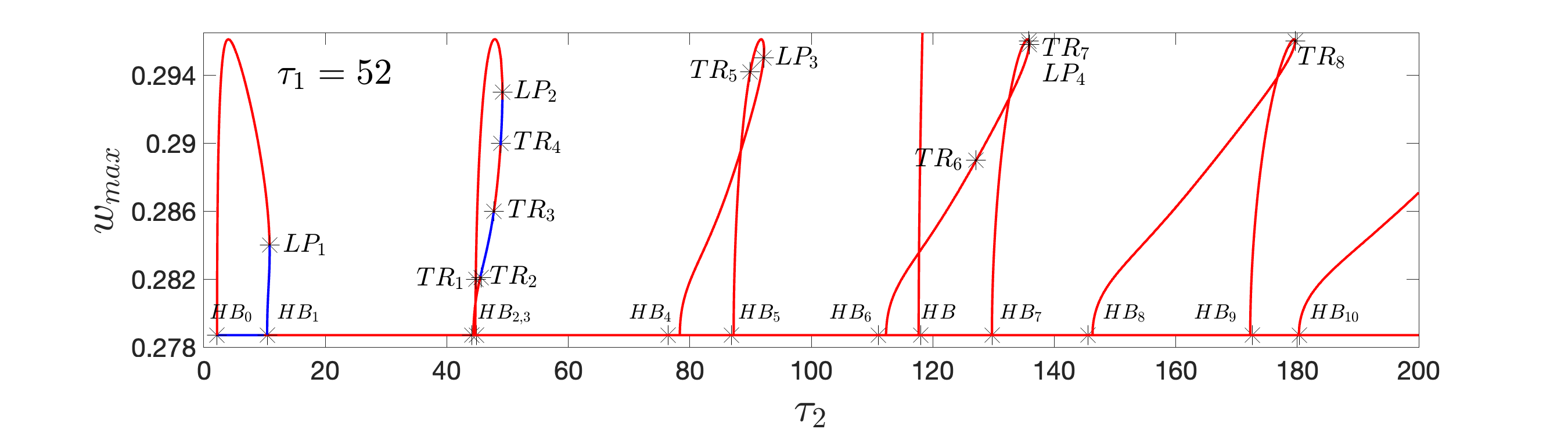
Figure 3: Bifurcation diagram with respect to the delay parameter $\tau_{2}$, with $\tau_{1}=52$. A sample of countably set of Hopf bifurcations is observed, with ten representative bifurcations labelled $HB_{i}$, $i=1,\dots,10$. The point labeled $HB$, located between $HB_{6}$ and $HB_{7}$, corresponds to the first $HB$ point shown in Figure 2(b). Periodic orbit branches emanate from each $HB_{i}$ and $HB$ point. Stable branches consisted of either periodic or steady-state orbits are indicated in blue, while unstable branches are shown in red. Asterisks mark torus ($TR$) and fold ($LP$) bifurcation points detected along periodic orbit branches.

Figure 3 presents the Hopf bifurcations observed for a fixed delay $\tau_{1}=52$. A primary Hopf bifurcation, denoted $HB_{0}$, occurs at $\tau_{2}=10.4208$ within the high-frequency interval $\omega\in\Omega_{2}$. This primary bifurcation is followed by a sequence of secondary Hopf bifurcations, labeled $HB_{i}$, $i=1,\dots,10$. An additional Hopf bifurcation, $HB$, is observed at $\tau_{2}=118.0674$ for some $\omega\in\Omega_{1}$, as depicted in Figure 2(b). The remaining secondary $HB_{i}$ bifurcations also occur within the low- and high-frequency intervals $\Omega_{1}$ and $\Omega_{2}$, as can be seen in Figure 2(b) and 2(c). We pay special attention to the high-frequency interval $\Omega_{2}$. The bifurcation diagram in Figure 3 validates the computations presented in Figure 2. Specifically, the criticality of the bifurcations in Figure 3 is consistent with the predictions derived from (13), as indicated by the asterisks in Figure 2(c).

Following the identification of the $\tau_{2}$ range associated with Hopf bifurcations, numerical continuation of equilibrium and periodic branches was performed using DDE-BIFTOOL [8]. Figure 3 displays these branches, including their stability properties (stable branches in blue, unstable branches in red), in a neighbourhood of the equilibrium point $E_{1}$, parameterised by $\tau_{2}\in[2,200]$ with $\tau_{1}=52$. The Hopf bifurcations marked with asterisks in Figure 2(c) were successfully located using DDE-BIFTOOL and correspond to the $HB_{i}$ points in Figure 3. Note that $HB_{0}$ is not shown in Figure 2(c) due to the figure’s scale. The $HB$ point in Figure 3 (between $HB_{6}$ and $HB_{7}$) corresponds to the first $HB\approx 117.3664$ in Figure 2(b). Slight numerical discrepancies were observed between the Hopf bifurcation points identified in Figures 2 and 3.

Furthermore, as illustrated in Figure 3, the analysis of periodic solution bifurcations revealed several torus ($TR$) and fold ($LP$) bifurcations. However, neither period-doubling bifurcations, characteristic of the Ruelle–Takens–Newhouse route to chaos [30], nor homoclinic bifurcations, indicative of the Shilnikov homoclinic chaos mechanism (see, e.g., [34, 13]), were detected within the explored parameter regime. This absence suggests that, if a chaotic regime exists, it likely arises through a different bifurcation scenario.

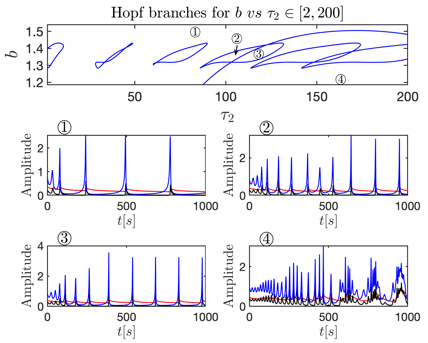
Figure 4: Top Panel: two-parameter continuation of Hopf bifurcation branches in the ($b$, $\tau_{2}$) parameter plane, with $\tau_{2}\in[2,200]$. Panels (1)-(4): temporal dynamics of the system variables for selected parameter values: (1) $\tau_{2}=80$, $b=1.5$; (2) $\tau_{2}=105$, $b=1.36$; (3) $\tau_{2}=115$, $b=1.36$; and (4) $\tau_{2}=160$, $b=1.2$. Other parameter values as in Table 1.

Two-parameter continuation was then performed, varying $b$ and $\tau_{2}$ for each Hopf bifurcation point within the range $\tau_{2}\in[2,200]$. The parameter $b$, related to the decay rate of motile to static bacteria, was chosen as the secondary bifurcation parameter due to its critical role in influencing the interplay of self-sustained oscillatory dynamics, as discussed in [18]. The results of this analysis are presented in the top panel of Figure 4. The two-parameter continuation of the Hopf branches reveals the formation of intersecting islands as $\tau_{2}$ increases, suggesting the potential for complex oscillatory behaviour. To shed light on this possibility, specific values of $b$ and $\tau_{2}$ were selected to explore key system behaviours over time. These values are: $\tau_{2}=80$, $b=1.5$ (point 1); $\tau_{2}=105$, $b=1.36$ (point 2); $\tau_{2}=115$, $b=1.36$ (point 3); and $\tau_{2}=160$, $b=1.2$ (point 4). The corresponding time series are shown in panels 1-4 of Figure 4. While the temporal dynamics depicted in panels 1 through 3 are qualitatively similar, panel 4 suggests the emergence of complex, non-periodic oscillations. This behaviour may result from the combined effect of small $b$ values and large $\tau_{2}$ values, given that $\tau_{1}$ remains fixed at 52.

5 Intermittent chaos in time delay QS system

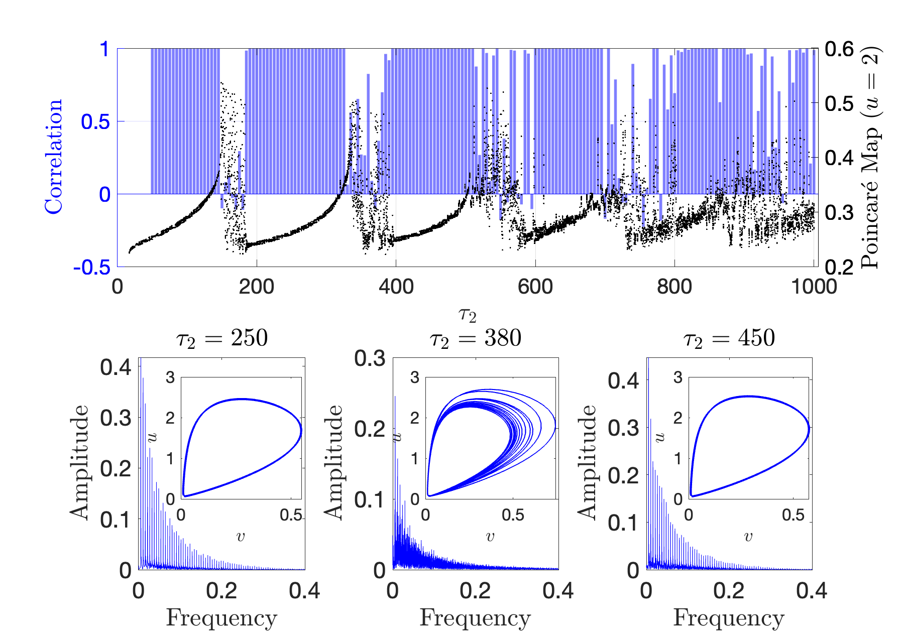
Figure 5: Upper row: Poincaré map computed on the cross-section $u=2$ (black dots) after transient time, as $\tau_{2}$ is slowly varied; Pearson correlation coefficient (blue bars) measuring the correlation between two initially nearby $w$-component orbits. Bottom row: frequency-amplitude plots and projections of representative orbits onto the ($u$, $v$) plane for three key distinct values of $\tau_{2}$; the central panel depicts a quasi-periodic orbit, while the left-hand and right-hand panels show stable periodic orbits. Other parameter values as in Table 1.

In the preceding section, the existence of periodic self-sustained oscillations was established for specific parameter values, as illustrated in Figure 4, panels 1-3. These periodic oscillations correspond to stable fixed points of the Poincaré map. Furthermore, as the time delay $\tau_{2}$ increases, the stability of these oscillations is altered, leading to a deformation of the oscillatory pattern, as observed in panel 4. This deformation suggests the emergence of complex, potentially non-periodic, dynamics.

To gain a comprehensive understanding of the oscillatory features governed by critical bifurcations, the Poincaré map of the time-delayed QS system (2) was computed over a substantial range of $\tau_{2}$ values, while holding $\tau_{1}$ constant. The first row of Figure 5 depicts the intersections of the state variable $u$ with the cross-section $u=2$ (black dots)—effectively, the Poincaré map—after transient time, as $\tau_{2}$ is slowly increased within the interval $\tau_{2}\in[2,1000]$ for fixed values of $\tau_{1}=52$ and $b=1.4$. As can be seen there, intervals of stable periodic solutions and complex quasi-periodic oscillations are interspersed until $\tau_{2}$ reaches a value sufficient to completely disrupt the periodic dynamics; see Figure 5, upper panel, $\tau_{2}\approx 700$. Beyond this point, the non-periodic oscillations suggest a chaotic regime, which is further explored in the bottom row of Figure 5 through frequency-amplitude plots and projections of distinguished orbits onto the $(u,v)$ phase plane. That is, for $\tau_{2}=250$, the Poincaré map indicates a stable periodic behaviour, which is corroborated by the well-defined orbit in the $(u,v)$ phase plane and the discrete frequency spectrum shown in the left-hand panel of the bottom row. When $\tau_{2}=380$, the dispersed Poincaré points and the dense orbit in the phase plane, coupled with the continuous frequency spectrum in the central panel, strongly indicate a chaotic regime. Finally, at $\tau_{2}=450$, the system returns to a stable periodic window, and the conclusions drawn for the case of $\tau_{2}=250$ apply.

To further validate the observed chaotic behaviour, the Pearson correlation coefficient [33] was computed and is displayed as blue bars in Figure 5, superimposed on the Poincaré map. Given two column vectors $x\in\mathbb{R}^{n\times 1}$ and $y\in\mathbb{R}^{n\times 1}$, with their respective averages $\overline{x}=\sum_{i=1}^{n}x_{i}/n$ and $\overline{y}=\sum_{i=1}^{n}y_{i}/n$, the Pearson linear correlation coefficient is given by

$$r_{x,y}=\dfrac{\sum\limits_{i=1}^{n}(x_{i}-\overline{x})(y_{i}-\overline{y})}{\sqrt{\sum\limits_{i=1}^{n}(x_{i}-\overline{x})^{2}}\sqrt{\sum\limits_{i=1}^{n}(y_{i}-\overline{y})^{2}}}.$$

This coefficient ranges from -1 to 1, where 1 indicates perfect positive correlation, -1 perfect negative correlation, and 0 no correlation. In this context, the correlation was calculated between two discretised trajectories of the $w$ state-component, initialised with a difference of approximately $10^{-9}$ units. As shown in Figure 5, the blue bars reveal strong correlation between $w$-orbits within the periodic regimes, while the correlation collapses to naught in the windows where chaotic behaviour dominates. This characteristic pattern is indicative of intermittent chaos, a phenomenon first described by Pomeau and Manneville in their analysis of the Lorenz system [25]. Intermittent chaos is a well-established phenomenon in time-delayed regulatory gene circuits, often attributed to the inherent delays in intracellular processes [32].

The comprehensive numerical simulations presented here provided further compelling evidence of the system’s richness dynamical repertoire. Such simulations not only corroborated the analytical predictions regarding the presence of self-sustained periodic oscillations, but also revealed the presence of intermittent chaotic behaviour as the delay parameters slowly vary. The intermittent nature of this chaotic regime, characterised by distinct phases of laminar flow punctuated by bursts of chaotic activity, strongly suggests a complex interaction between the destabilised steady-state and the emerging oscillatory modes. That is, the scheme that found and illustrated in Figure 5 corresponds to Type-II intermittency, within the Pomeau–Manneville classification design, which represents a distinct pathway to chaotic dynamics characterised by the irregular, intermittent switching between laminar phases and bursts of chaotic activity. A key distinguishing feature of Type-II intermittency is its association with a subcritical Hopf bifurcation. Specifically, as a system parameter traverses a critical value, a complex conjugate pair of eigenvalues associated with a stable periodic orbit crosses the imaginary axis, destabilising such orbit. The complex monodromic eigenvalues at the bifurcation point are of the form $\mu=\left(1+\varepsilon\right)e^{i\theta}$, where the local Poincare map can be described, in polar coordinates, by its normal form

$$\left\{\begin{array}[]{l}r_{n+1}=\left(1+\varepsilon\right)r_{n}+ar^{3}_{n}\,,\\[4.30554pt] \theta_{n+1}=\theta_{n}+c+br^{2}\,,\end{array}\right.$$

where $a,b,c\in\mathbb{R}$ are constant, and Type-II intermittency occurs for $\varepsilon>0$, see [6]. This destabilisation gives rise not to a global chaotic attractor, but rather to a repeller in the vicinity of the now-unstable periodic orbit. The dynamics near this repeller are inherently chaotic, due to its unstable nature provided by positive Lyapunov exponents, here described by means of the geometric transversality parameter (13) and confirmed by computations shown in Figures 2 and 3. Orbits are intermittently “injected” into the neighbourhood of this repeller, leading to a burst of chaotic behaviour. Following this excursion into the chaotic region, the trajectory is subsequently re-injected into the phase space region previously occupied by the stable periodic orbit, resulting in a return to laminar periodic flow as is illustrated in Figure 5, upper row. The average durations of these laminar phases, $\bar{l}$, are statistically distributed, typically exhibiting a power-law scaling with the distance of the bifurcation parameter from its critical value, which is $\bar{l}\sim\varepsilon^{-1/2}$, see [6]. The essential mechanism underlying this phenomenon is the interplay between the destabilised periodic orbit (and its associated repeller) and the reinjection process that governs the transitions between laminar and chaotic phases.

6 Concluding Remarks

This present study has investigated the profound influence of distinct time delays on the dynamical behaviour of a QS-inspired system, employing a nonlinear delay differential equation framework. Specifically, we modelled a system comprising motile and static bacterial subpopulations, each exhibiting distinct response times to autoinducer signals, thereby introducing two independent delay parameters, $\tau_{1}$ and $\tau_{2}$. This approach acknowledges the inherent temporal lags associated with the intricate network of biochemical processes underpinning QS, which may include signal production, transport diffusion features, and cellular response.

Our analysis commenced explicitly incorporating two distinct delays, building upon a well-established activator-inhibitor framework to effectively represent the dynamic interplay between motile (activator) and static (inhibitor) bacterial populations. Subsequently, we conducted a detailed analysis of the existence and local stability properties of the system’s steady-states. Upon deriving the pseudo-characteristic polynomial and meticulously examining the conditions governing the emergence of purely imaginary eigenvalues, we established the potential for Hopf bifurcations as the delay parameters were slowly varied. Our findings show that the presence of multiple delays, particularly when characterised by significant disparities in magnitude, can dramatically alter the system’s stability features and promote the emergence of complex nonlinear oscillatory behaviour. Specifically, we have demonstrated that the steady-states $E_{1}$ and $E_{2}$ can undergo Hopf bifurcations, losing stability as the difference between the delays, $h=\tau_{1}-\tau_{2}$, is increased, while the steady-state $E_{3}$ robustly maintains its stability across the explored range of delay values. The observed difference in the magnitude of $h$ required to induce instability in $E_{1}$ compared to $E_{2}$ suggests a complex and nuanced interplay between the two distinct delays and the inherent dynamical properties of each respective steady-state.

The results presented in this study make a significant contribution to our fundamental understanding of the role of time delays in shaping the dynamics of QS systems. Upon explicitly incorporating distinct delays for different state-components, we have shown how temporal factors can dramatically influence system stability and give rise to a spectrum of complex dynamical behaviours, including intermittent chaos. These findings offer crucial contributions to our understanding of microbial communication and have the potential to inform the development of innovative strategies for targeted manipulation of QS systems. Future research directions could explore an extension of the current model to incorporate spatial heterogeneity and more complex interaction topologies, important factors that are beyond the scope of the present analysis and will be addressed in future work. Moreover, the insights gained from this study may prove invaluable in the design and engineering of synthetic biological systems where precise control of gene expression and population dynamics is paramount.

In summary, we have exhibited the impact of heterogeneous time delays on QS dynamics. Upon modelling subpopulation-specific response times, we have revealed the complex interplay between temporal heterogeneity, stability, and emergent oscillations. These findings promote our understanding of delay-mediated regulation and may offer a foundation for developing control strategies in synthetic biology, emphasising the necessity of considering temporal heterogeneity in certain complex biological systems.

Moreover, the presented investigation has yielded key insights into the temporal dynamics of QS; however, the inherent spatial heterogeneity arising from transport phenomena constitutes a critical determinant of system behaviour. To achieve a more comprehensive and predictive understanding, future research will extend the current model to explicitly incorporate transport dynamics. This integration is essential for capturing the spatiotemporal complexity inherent in QS systems.

References

- [1] M. Barbarossa, C. Kutter, A. Fekete, and M. Rothballer, A delay model for quorum sensing of Pseudomonas putida, BioSystems, 102 (2020), pp. 148–156.
- [2] R. C. Calleja, A. R. Humphries, and B. Krauskopf, Resonance phenomena in a scalar delay differential equation with two state-dependent delays, SIAM Journal on Applied Dynamical Systems, 16 (2017), pp. 1474–1513.
- [3] M. Chen, J. Ji, H. Liu, and F. Yan, Periodic Oscillations in the Quorum-Sensing System with Time Delay, International Journal of Bifurcation and Chaos, 30 (2020).
- [4] M. Chen, H. Liu, and F. Yan, Oscillatory dynamics mechanism induced by protein synthesis time delay in quorum-sensing system, Physical Review E, 99 (2019).
- [5] M. Chen, H. Liu, and F. Yan, Modelling and analysing biological oscillations in quorum sensing networks, IET Syst. Biol., 14 (2020), pp. 190–199.
- [6] S. Elaskar and E. del Río, Review of Chaotic Intermittency, Symmetry, 15 (2023), p. 1195.
- [7] M. Elowitz and S. Leibler, A synchronized oscillatory network oftranscriptional regulator, Nature, 403 (2000), pp. 335–338.
- [8] K. Engelborghs, T. Luzyanina, and D. Roose, Numerical bifurcation analysis of delay differential equations using dde-biftool, ACM Transactions on Mathematical Software (TOMS), 28 (2002), pp. 1–21.
- [9] P. Fergola, M. Cerasuolo, and E. Beretta, An allelopathic competition model with quorum sensing and delayed toxicant production, Mathematical Biosciences & Engineering, 3 (2006), p. 37.
- [10] P. Fergola, J. Zhang, M. Cerasuolo, and Z. Ma, On the influence of quorum sensing in the competition between bacteria and immune system of invertebrates, in AIP Conference Proceedings, vol. 1028, American Institute of Physics, 2008, pp. 215–232.
- [11] M. R. Frederick, C. Kuttler, B. A. Hense, and H. J. Eberl, A mathematical model of quorum sensing regulated eps production in biofilm communities, Theoretical Biology and Medical Modelling, 8 (2011).
- [12] J. García-Ojalvo, M. B. Elowitz, and S. H. Strogatz, Modeling a syntheticmulticellular clock: repressilators coupled by quorum sensing, Proc. Natl. Acad. Sci. USA, 30 (2004), pp. 10955–10960.
- [13] S. V. Gonchenko, D. V. Turaev, P. Gaspard, and G. Nicolis, Complexity in the bifurcation structure of homoclinic loops to a saddle-focus, Nonlinearity, 10 (1997), p. 409.
- [14] A. Goryachev, Design principles of the bacterial quorum sensing gene networks, Wiley Interdiscip Rev Syst Biol Med., 1 (2009), pp. 45–60.
- [15] K. Gu, S.-I. Niculescu, and J. Chen, On stability crossing curves for general systems with two delays, Journal of mathematical analysis and applications, 311 (2005), pp. 231–253.
- [16] M. R. Guevara, L. Glass, M. C. Mackey, and A. Shrier, Chaos in neurobiology, IEEE Transactions on Systems, Man, and Cybernetics, SMC-13 (1983), pp. 790–798.
- [17] B. K. Hammer and B. L. Bassler, Quorum sensing controls biofilm formation in vibrio cholerae, Molecular microbiology, 50 (2003), pp. 101–104.
- [18] M. Harris, V. Rivera-Estay, P. Aguirre, and V. Breña-Medina, Multiple Local and Global Bifurcations and Their Role in Quorum Sensing Dynamics. arXiv:2409.02764, 2025.
- [19] C. Kuttler and A. Maslovskaya, Hybrid stochastic fractional-based approach to modeling bacterial quorum sensing, Applied Mathematical Modelling, 93 (2021), pp. 360–375.
- [20] M. Lakshmanan and D. V. Senthilkumar, Dynamics of nonlinear time-delay systems, Springer Science & Business Media, 2011.
- [21] J. Lee, J. Wu, Y. Deng, J. Wang, C. Wang, J. Wang, C. Chang, Y. Dong, P. Williams, and L.-H. Zhang, A cell-cell communication signal integrates quorum sensing and stress response, Nature chemical biology, 9 (2013), p. 339.
- [22] J. Lewis, Autoinhibition with transcriptional delay: a simple mechanism for the zebrafish somitogenesis oscillator, Current Biology, 13 (2003), pp. 1398–1408.
- [23] G. J. Lyon and R. P. Novick, Peptide signaling in staphylococcus aureus and other gram-positive bacteria, Peptides, 25 (2004), pp. 1389–1403.
- [24] M. C. Mackey and L. Glass, Oscillation and chaos in physiological control systems, Science, 197 (1977), pp. 287–289.
- [25] P. Manneville and Y. Pomeau, Intermittency and the lorenz model, Physics Letters A, 75 (1979), pp. 1–2.
- [26] W. Michiels and S.-I. Niculescu, Stability and stabilization of time-delay systems: an eigenvalue-based approach, SIAM, 2007.
- [27] N. A. Monk, Oscillatory expression of hes1, p53, and nf-b driven by transcriptional time delays, Current Biology, 13 (2003), pp. 1409–1413.
- [28] M. Mukherjee and B. L. Bassler, Bacterial quorum sensing in complex and dynamically changing environments, Nat Rev Microbiol., 17 (2019), pp. 371–382.
- [29] K. H. Nealson, T. Platt, and J. W. Hastings, Cellular control of the synthesis and activity of the bacterial luminescent system, Journal of bacteriology, 104 (1970), pp. 313–322.
- [30] S. Newhouse, D. Ruelle, and F. Takens, Occurrence of strange AxiomA attractors near quasi periodic flows on , , Communications in Mathematical Physics, 64 (1978), pp. 35–40.
- [31] J. Perez-Velazquez, B. Quinones, B. A. Hense, and C. Kuttler, A mathematical model to investigate quorum sensing regulation and its heterogeneity in pseudomonas syringae on leaves, Ecological Complexity, 21 (2015), pp. 128–141.
- [32] Y. Suzuki, M. Lu, E. Ben-Jacob, and J. N. Onuchic, Periodic, quasi-periodic and chaotic dynamics in simple gene elements with time delays, Scientific reports, 6 (2016), p. 21037.
- [33] R. Walpole, R. Myers, and S. Myers, Probabilidad y estadística para ingeniería y ciencias, Pearson educación, 2012.
- [34] S. Wieczorek and B. Krauskopf, Bifurcations of n-homoclinic orbits in optically injected lasers, Nonlinearity, 18 (2005), p. 1095.
- [35] S. Yanchuk and P. Perlikowski, Delay and periodicity, Physical review E, 79 (2009), p. 046221.
- [36] C.-K. Yap et al., Fundamental problems of algorithmic algebra, vol. 49, Oxford University Press Oxford, 2000.
- [37] Y. Zhang, H. Liu, F. Yan, and J. Zhou, Oscillatory dynamics of p38 activity with transcriptional and translational time delays, Scientific reports, 7 (2017), pp. 1–11.
- [38] Y. Zhang, H. Liu, and J. Zhou, Oscillatory expression in escherichia coli mediated by micrornas with transcriptional and translational time delays, IET Systems Biology, 10 (2016), pp. 203–209.
- [39] Z. Zhang, Y. Suo, J. Peng, and J. Zhang, Analysis of a periodic bacteria-immunity model with delayed quorum sensing, Computers and Mathematics with Applications, 56 (2008), pp. 2834–2847.
- [40] Z. Zhonghua, S. Yaohong, Z. Juan, and P. Jigeng, A bacteria-immunity system with delayed quorum sensing, Journal of Applied Mathematics and Computing, 30 (2009), pp. 201–217.