Localization and entanglement entropy
in the Discrete Non-Linear Schrödinger Equation

Abstract

In this work we perform an accurate numerical study of the very peculiar thermodynamic properties of the localized high-energy phase of the Discrete Non-Linear Schrödinger Equation (DNLSE). A numerical sampling of the microcanonical ensemble done by means of Hamiltonian dynamics reveals a new and subtle relation between the presence of the localized phase and a non-trivial behaviour of entanglement entropy. Our finding that the entanglement entropy grows as $S_{\text{ent}}(N)\sim\log(N)$ beautifully encodes the lack of additivity in the DNLSE non-thermal localized phase and reveals how a property so far believed peculiar of purely quantum systems may characterize even certain classical frameworks.

I Introduction

The dynamic and thermodynamic properties of the high-energy phase of the Discrete Non-Linear Schrödinger Equation (DNLSE), a classical system that works as an effective description for a bosonic condensate wavefunction on a lattice [1], have been debated for a long time. As for high energy phase we refer to values of the energy per lattice site larger than the threshold value $e_{\text{th}}=2a^{2}$, where $a$ denotes the mass per lattice site of a bosonic condensate. According to the seminal results of [2], the parabola $e_{\text{th}}=2a^{2}$, which is also represented in Fig.1 here denotes the critical line above which the grand-canonical ensemble becomes ill-defined. Since then, for a couple of decades there has been no equilibrium thermodynamic calculation capable of tackling the regime $e>2a^{2}$, so that different and controversial speculations have been made about the nature of this phase. Numerical simulations of the DNLSE dynamics in this high energy regime provided several and incontrovertible evidences that strongly localized structures (breathers) are stable or, to say the least, metastable on gigantic timescales which exceed the simulation time even on modern computers [3]. Numerical simulations in the regime $e>2a^{2}$ provided compelling evidence of a phenomenon which cannot be described within the grand-canonical ensemble: the presence of negative temperatures [3]. We show the result of numerical simulations which do not suffer this limitation since are performed in the microcanonical ensemble, here the temperature is an observable which can be either positive or negative since it is directly measured as

$$\beta=\frac{1}{T}=\frac{\partial S(E)}{\partial E},$$ (1)

where $S(E)$ is the microcanonical entropy as a function of the energy and where we have assumed $k_{B}=1$. The microcanonical definition of temperature in Eq. (1) clearly does not suffer the limitations that the concept of temperature has in the canonical ensemble. An account on negative temperatures has been recently provided in [4]: for a systems with compact domain variables negative temperatures can be consistently defined even in the canonical ensembles, since the canonical weight $e^{-\beta H}$ is finite even when $\beta<0$. On the contrary, the same is not true for locally unbounded variables, which is the case for the DNLSE. Recently, an effective grand canonical description for delocalized metastable states at negative temperature was provided in [5], while a consistent thermodynamic approach capable of accounting for both localized states and negative temperatures has been more controversial.

By means of a large-deviation exact estimate of the microcanonical partition function in the regime $e>2a^{2}$, it has been possible to provide a complete and precise account of the localized and negative-temperature phase also from a thermodynamic point of view [6, 7]. Differently from what happens in the case of long-range interacting systems, where the terminology lack of ensembles equivalence refers to the different predictions drawn from the two ensembles [8], for what concerns the localized phase of the DNLSE it turns out that a stronger meaning to the concept of ensemble non-equivalence must be assumed. The localized phase of the DNLSE only exists in the microcanonical ensemble, namely it can be reached only by directly fixing the energy to a high enough value and cannot be reached in any way by adjusting the average energy by means of a thermostat homogeneously coupled to the system. However, this should not be considered as a surprise or a peculiar situation. It is well-known from Ruelle’s monograph on statistical mechanics [9] that, when localization or condensation phenomena occur, the equivalence between statistical ensembles may be broken. In particular, the main finding of [6, 7] was that the localized phase of the DNLSE is genuine thermodynamic equilibrium phase characterized by negative absolute temperatures. The large-deviation calculation of the microcanonical entropy presented therein was capable of claryfing first-order features of the localization transition in the DNLSE at the price of only one relevant, even though standard in the high energy regime (see also [10]), approximation: the neglecting the hopping term in the Hamiltonian.

On the basis of the framework just outlined, we can now clearly state the two main purposes of the present work. First of all we will present here a numerical evidence validating the microcanonical results of [6, 7] on the participation ratio and negative temperature, in particular we will find a confirmation of the predicted finite-size scalings. Secondly, and most importantly, we will show how to characterize ensemble inequivalence, localization and the breakdown of additivity by measuring a new observable: the entanglement entropy $S_{\text{ent}}(N)$ as a function of lattice size $N$. In the present work we show how the condensate wavefunction, which has a quantum origin but is formally treated as a classical field obeying standard classical statistical mechanics, in the localized phase presents features which are totally analogous to those of a true quantum system: a non-trivial scaling with system size of the entanglement entropy. From the physical point of view this observation tells us that in the localized negative-temperature phase, due to subtle non-local correlations, the system really behaves as a true quantum phase. We will show how both numerical simulations of the full Hamiltonian dynamics and analytical estimates based on the results of [6, 7] agree on a scaling with system size of entanglement entropy which in the localized phase is of the kind

$$S_{\text{ent}}(N)\sim\log(N),$$ (2)

while in the homogeneous phase where canonical and microcanonical ensembles are equivalent and temperature is positive is trivial, $S_{\text{ent}}\sim\text{const}$.

The presentation of the results just mentioned is divided as follows. In Sec. II we present the model, recalling its phase diagram, and discuss the simulation protocol. In Sec. III we will present the numerical results from Hamiltonian dynamics on the finite-size scaling of the participation ratio $Y_{2}(N)$ and the microcanonical temperature $T_{\text{micro}}(N)$ in the homogeneous and the localized phase. Sec. IV will be then devoted to the presentation of results on the entanglement entropy. A more detailed discussion on the following points is left for the Appendices: characterization of the thermodynamic observables in the pseudo-localized phase discovered in [6], Sec. App 1; the inconsistency of local definitions of temperature in localized phase of the DNLSE, Sec. App 2; hints that the localization transition in the DNLSE has features of an ergodicity-breaking transition, Sec. App 3; details on the temperature observable in the microcanonical ensemble, Sec. App 4.

II Model and Methods

In this manuscript we study numerically the Hamiltonian dynamics of the Discrete Non-Linear Schrödinger Equation with two main goals: confirm the analytical predictions on thermodynamics of [6, 7] and study the behavior of entanglement entropy. The DNLSE is a set of classical Hamiltonian equations describing the behavior of a macroscopic field of quantum origin, the condensate wave-function $z_{j}\in\mathbb{C}$:

$$i\dot{z_{j}}=-\frac{\partial\mathcal{H}}{\partial z_{j}^{*}}=-(z_{j+1}+z_{j-1})-2|z_{j}|^{2}z_{j}\,,$$ (3)

where the index $j$ labels the sites of a one-dimensional lattice of size $N$ and $i$ is the imaginary constant. Due to global gauge invariance $z_{j}\rightarrow z_{j}e^{i\alpha}$ the dynamics of Eq. (3) conserves the total mass $\mathcal{A}$ in addition to the total energy $\mathcal{H}$, the two quantities reading (in polar representation $z_{j}=\rho_{j}e^{i\phi_{j}}$) respectively as:

$$\mathcal{A} =\sum_{j=1}^{N}|z_{j}|^{2}\,\equiv\sum_{j=1}^{N}\,\rho_{j}^{2}$$ (4)

$$\mathcal{H} =\sum_{j=1}^{N}(z_{j}^{*}\,z_{j+1}\,+\,z_{j}\,z_{j+1}^{*})\,+\,\sum_{j=1}^{N}|z_{j}|^{4}$$

$$=2\sum_{j=1}^{N}\rho_{j}\rho_{j+1}\cos(\phi_{j+1}-\phi_{j})\,+\,\sum_{j=1}^{N}|\rho_{j}|^{4}$$ (5)

We denote with $E$ and $A$ the real values attributed to the observables $\mathcal{H}$ and $\mathcal{A}$, with $e=E/N$ and $a=A/N$ the corresponding values per lattice site. Since $A$ and $E$ are the two conserved quantities which characterize the DNLSE dynamics, it is natural to retain them as control parameters also for the thermodynamics and draw a phase diagram in the plane $(a,e)$. According to the results of [6, 7] at large but finite values of $N$ one can identify in the phase diagram of Fig. 1 the following three regions above the low energy forbidden one (gray):

• Homogeneous phase: $e<e_{\text{th}}(a)$
  The distribution of the condensate wave-function on the lattice is homogeneous, the temperature is positive, and the ensembles are equivalent. Thermodynamics is standard, i.e., by raising the temperature both energy and entropy increase. In this regime we will show in the present work that the entanglement entropy has the trivial behavior which can be traced in any additive system: it does not depend on system size.

• Pseudo-localized phase: $e_{\text{th}}(a)<e<e_{c}(a,N)$
  There can be peaks in the condensate wave-function distribution on the lattice, but without concentration of a finite fraction of the total mass on a single site. The system can be described only in the microcanonical ensemble, temperature is negative and thermodynamics is “non-standard”: the increase of system energy induces a decrease of entropy, due to an incresing tendency to localize rather than share energy.

• Localized phase: $e>e_{c}(a,N)$
  Temperature is negative and the system is in the localized phase where a finite fraction of the total mass is concentrated in $\mathcal{O}(1)$ sites. The ”anomalous” thermodynamics of the pseudo-localized phase is finally established as the dominant behavior: upon increasing energy the system becomes more and more localized and the entropy becomes smaller and smaller. Like a black hole, one (or few) gigantic breather eat all the additional energy which is fed to the system, producing a shrinking of phase space and a decrease of entropy. We will further clarify the anomalous thermodynamic nature of this regime in this work by showing that the entanglement entropy increases logarithmically like the size of the system, indicating the presence of non-trivial global correlations and putting on firm conceptual grounds the impossibility to provide any local definition of temperature in the system.

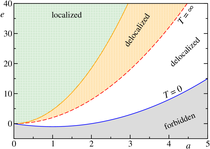
Figure 1: Microcanonical phase diagram of the DNLSE model. Solid blue line identifies the ground state $e=a^{2}-2a$ at $T=0$ (see [2] for details) below which there are forbidden states. The red dashed line refers to $e_{\text{th}}(a)=2a^{2}$ and is characterized by infinite temperature. Above it $T$ is negative: delocalized states are contained in the orange region $e_{\text{th}}(a)<e<e_{c}(a,N)$, while localized ones for $e>e_{c}(a,N)$ are highlighted in green color. The solid orange curve here refers to $e_{c}(a,N)=e_{\text{th}}(a)+11.05\,a^{2}N^{-1/3}$ with $N=100$, according to [6, 7].

In the calculation of the microcanonical partition function we considered only one approximation: we have neglected the hopping term in Eq.(5), thus writing $\Omega$ as

$$\Omega_{N}(A,E)=$$

$$\int\prod_{i=1}^{N}dz_{i}~\delta\left(A-\sum_{i=1}^{N}|z_{i}|^{2}\right)\delta\left(E-\sum_{i=1}^{N}|z_{i}|^{4}\right).$$ (6)

Let us recall the argument which allows to drop the hopping terms [6, 7]: close to and above the infinite-temperature line $e_{\text{th}}(a)$ one can safely assume that the phases of the condensate wave-function at different lattice sites are iid random variables. This implies that the first sum in Eq. (5) is a sum of terms with alternating sign, so that, while the on-site quartic term of the energy gives a contribution of order $N$, the hopping term gives a contribution of order $\sqrt{N}$. Clearly, such an approximation is not rigorously under control, in particular considering the fact that, from the resulting simplified partition function, we have computed sub-leading contributions in $N$ to the microcanonical entropy. This is the reason why the exact results (under the just-mentioned approximation) presented in [6, 7] need to be validated by numerical simulations of the full Hamiltonian dynamics where the hopping term is retained.

The present study of the DNLSE behavior has two main goals: confirm the thermodynamic scenario on the localization transition emerging from the exact asymptotic estimates of [6, 7] and provide new insights on the system by studying the entanglement entropy. In order to do that we need the precise knowledge of the energy values at which the system is either in the homogeneous and in the localized phase. From the result of [6, 7] we know that the threshold value of the energy $e_{\text{th}}$ at which the description of the system in terms the canonical ensemble breaks down, already found in [2], does not coincide with the critical energy $e_{c}(N)$ at which localization takes place at large but finite $N$. Therefore, since we have to deal with numerical simulations at finite values of $N$, it is crucial to known $e_{c}(N)$ in order to choose appropriately the energy where the system is in the localized phase. According to the large deviations estimates of [6, 7] these two values have the following relation:

$$e_{c}(a,N)=e_{\text{th}}(a)+\frac{\zeta_{c}(a)}{N^{1/3}}\,,$$ (7)

where both $e_{\text{th}}(a)=2a^{2}$ and $\zeta_{c}(a)$ are analytic functions of $a$. The explicit expression of $e_{\text{th}}(a)=2a^{2}$ has been found both in  [2] and in [6], whereas the explicit formula of $\zeta_{c}(a)$ is a result of [6]. In particular for $a=1$ we have

$$e_{\text{th}}(a=1) =2$$

$$\zeta_{c}(a=1) =11.05.$$ (8)

Let us notice that while the threshold value $e_{\text{th}}(a)=2\,a^{2}$ can be obtained both from an exact estimate in the grandcanonical ensemble [2] and from the canonical calculation of [6], the critical value $e_{c}(a,N)$ where localization exactly takes place can be obtained only from the microcanonical calculation. Its precise knowledge is crucial for the purpose of this paper, allowing a precise choice of initial conditions either in the homogeneous positive temperature phase or in the localized phase for any choice of lattice size $N$. The values of $e_{c}(N)$ at the different sizes $N$ considered in the present work are listed in Tab. 1. For energies between these two critical values, i.e., $e_{c}{\text{th}}<e<e_{c}$, the system displays a pseudo-condensed phase, in which the control of finite-size effect is more subtle. In order to keep self-contained the discussion of the main results, we report details of this regime in App 1.

Looking at the phase diagram in Fig. 1 it is clear that one can arbitrarily choose any finite value of $a$ and then study the properties of the localized phase by increasing $e$. For this reason, we have fixed the condensate mass to $a=1$ in our numerical simulation and then varied $e$. Different choices of $a$ are immaterial: the high-energy region is invariant under a uniform rescaling of norms, so that $a$ is essentially a unit of measure and that equilibrium properties therein depend on $e/a^{2}$ only.

The goal of this work is the characterization of three main observables and their dependence on the lattice size $N$: the participation ratio $Y_{2}$, the microcanonical temperature $T^{-1}=\partial S/\partial E$, and the entanglement entropy $S_{\text{ent}}$. The crucial point of our analysis is that, in order to sample the equilibrium value of these observables by means of the Hamiltonian dynamics, we need to choose the initial conditions in the corresponding phase. The protocol followed is described in the next subsection. All numerical simulations have been performed making use of a symplectic 4th order integration algorithm of Yoshida type [11, 12] with timestep $dt=10^{-2}$, which ensures conservation of energy to order $dt^{4}$.

$~~e_{c}(1,N)~~$	$~~~N~~~$
4.19	128
3.74	256
3.38	512
3.10	1024
2.87	2048
2.69	4096

Table 1: Numerical values of the critical energy $e_{c}(a,N)$ for the localization transition for $a=1$, estimated energy of the “metastable” phase (negative temperature, no localization) and corresponding $N$.

II.1 Initial conditions

In order to study the localized phase of the DNLSE with Hamiltonian dynamics we take advantage of the precise knowledge of equilibrium phases features gathered from [6, 7], which allows us to choose initial conditions at the appropriate energy $e$ for each lattice size $N$ in order to be either in the homogeneous or in the localized phase. This task is particularly delicate in the present context, since at high energies, due to the lack of a canonical description, a standard ”thermal” initial condition is inappropriate and the presence of the localized state must be included already in the initial state, respecting at the same time the macroscopic constraints on the condensate total mass and energy. In particular, when $e>e_{\text{th}}$, the correct procedure is to assign the initial value of $|z_{j}|^{2}=\rho_{j}$ according to the infinite temperature canonical distribution on $N-1$ lattice sites and then to place the remaining mass on the last site. This means that the initial values of $\rho_{j}$, for $j=1,\cdots,N-1$ are extracted from the Poisson-like distribution

$$p(\rho_{j}^{2})=\frac{e^{-\rho_{j}^{2}/a}}{a}$$ (9)

while a “breather” containing the excess energy is placed on a randomly chosen site on the lattice, for which we considered periodic boundary conditions. On this site the value of the density is given by the expression

$$\rho_{N}^{2}=\sqrt{e-e_{\text{th}}(a)}~N^{1/2}\,.$$ (10)

The phases $\phi_{j}$ are randomly initialized from a uniform probability distribution in the interval $[0,2\,\pi]$. The values of $\rho_{j}^{2}$, initially sampled from the distribution in Eq. (9), are finally rescaled in order to fulfill the macroscopic constraints on mass and energy:

$$A=a~N=\sum_{j=1}^{N}\rho_{j}^{2} \qquad\qquad E=e~N=\sum_{j=1}^{N}\rho_{j}^{4}$$ (11)

This sort of initial conditions is obviously stable with respect to Hamiltonian dynamics in the localized phase. In the positive temperature phase, on the other hand, the system is initialized according to the following procedure: first, similarly to the localized phase, we initialize the system at infinite temperature, following the distribution of Eq. (9). Then, using a phase update algorithm, we progressively decrease the energy down to the desidered value $e<e_{\text{th}}$. The phase update algorithm works by selecting a random site on the lattice and changing its phase by drawing a new value from $[-\pi,\pi]$. If the new phase decreases the energy density, it is accepted; otherwise, it remains unchanged. This procedure is repeated until the desired energy density $e$ is reached.

III Thermodynamic Observables

In this section it is presented the numerical validation of the main thermodynamic results from [6] on the participation ratio and the finite-size scaling of the DNLSE microcanonical temperature in the localized phase. In particular we focus here on the homogeneous and on the fully localized regimes, corresponding respectively to $e<e_{\text{th}}$ and $e>e_{c}$, leaving the discussion of the pseudo-localized phase at $e_{\text{th}}<e<e_{c}$ in App 1.

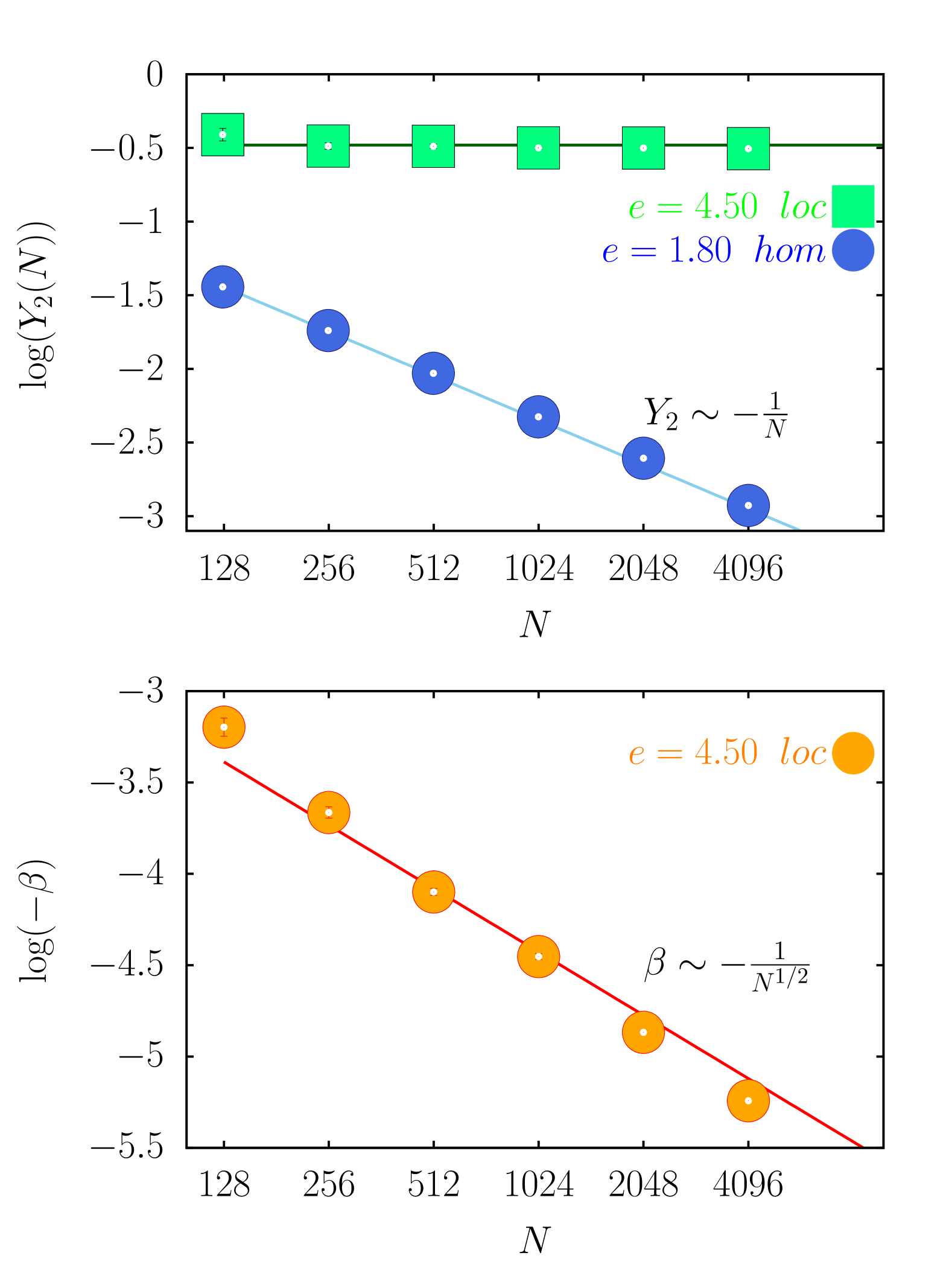
Figure 2: Upper panel: Finite-size scaling of the participation ratio $Y_{2}(N)$ of the DNLSE for $a=1$ and different energy densities $e$. Statistical expectations are computed as time averages in the time interval $10^{5}$-$10^{6}$. Error bars are the standard deviation of fluctuations, sampled at intervals $\Delta t=10$, in the measurement window. Lower panel: Finite-size scaling of minus the inverse temperature, $-\beta$, vs. $N$ in the metastable and stable localized phases. The system has been initialized with an artificial breather added to an infinite temperature background, with $a=1$. The running time of the simulations is $\Delta\tau=1.5\times 10^{3}$, and the microcanonical temperature has been measured globally across all the sites of the system. The uncertainties have been evaluated as the standard deviation of the temperature measurements taken at every $d\tau=10$ as the simulations progress. The red line corresponds to the fit with the theoretical prediction.

III.1 Participation Ratio

The order parameter which signals the presence of a localized phase is the participation ratio $Y_{2}(N)$, which is defined as follows:

$$Y_{2}(N)=\left\langle\frac{\sum_{j=1}^{N}\varepsilon_{j}^{2}}{\left(\sum_{j=1}^{N}\varepsilon_{j}\right)^{2}}\right\rangle_{A,E},$$ (12)

where $\left\langle~\right\rangle_{A,E}$ denotes the microcanonical average and we have introduced the shorthand notation $\varepsilon_{j}=\rho_{j}^{4}$. The analytic calculation reported in [6] provides precise estimates about the dependence of $Y_{2}(N)$ on the system size $N$ in two regimes, the localized phase at $e>e_{c}$ and the the homogeneous phase at $e<e_{\text{th}}$. For intermediate values of the energy, $e_{\text{th}}<e<e_{c}$, a solid argument is offered in [6] only for differences of order $e-e_{\text{th}}\sim N^{-1/2}$, but not for differences in the so-called matching regime, $e-e_{\text{th}}\sim N^{-1/3}$, where one can only guess a scaling of the kind $e-e_{\text{th}}\sim N^{-\gamma}$, with $\gamma<1$.

It is also worth recalling that this intermediate regime shrinks to zero in the thermodynamic limit, since $\lim_{N\rightarrow\infty}e_{c}(N)=e_{\text{th}}$.

In the upper panel of Fig. 2 is reported the dependence on $N$ of $Y_{2}(N)$ for the two energy regimes just mentioned, obtained by fixing the condensate mass per lattice site to $a=1$. For $e=1.8$ (blue circles) the system is in the positive temperature region (recall that $e_{\text{th}}=2$) and numerical simulations confirm the reliability of the analytic estimate, i.e. $Y_{2}(N)$ is actually found to decay as $N^{-1}$, as is emphasized by the straight blue line. For the localized phase at $e=4.5>e_{c}$ (green squares) there is also a compelling evidence of the agreement between the simulations of Hamiltonian dynamic and the analytic estimates of [6, 7], i.e., $Y_{2}(N)$ approaches a constant value $Y_{2}(\infty)$ for large $N$, as is emphasized by the straight green line, which is compatible with asymptotic estimate $Y_{2}(\infty)=(e-e_{th})^{2}/e^{2}$ [13]. The validation of the theoretical predictions presented here and obtained from the full Hamilton dynamics is not redundant with respect to the agreement between theory and numerics already found in [13, 14] by means of stochastic algorithms, since also in this last case the hopping terms were neglected.

III.2 Negative Temperature

Here we present evidence from numerical data that in the localized phase, $e>e_{c}(N)$, there is an agreement between the measure of negative temperature along Hamiltonian dynamics and the analytical estimate of [6, 7]. Let us stress that, in the microcanonical ensemble, temperature is an observable, not a parameter. For the system considered here, two issues arise in its measurement: one related to the specific Hamiltonian defining the DNLSE and another to the phase of interest. The first issue stems from the non-separability of the DNLSE Hamiltonian (5) [15, 16, 17, 18], as its canonical conjugate momentum is proportional to $z_{j}^{*}$ rather than $\dot{z}_{j}$. It is therefore not possible by construction to define operatively temperature as the average kinetic energy of the systems, as it is usually done in molecular dynamics simulations, due to the non-separability of the Hamiltonian. The only definition of temperature which can be exploited in this context is the microcanonical definition: $T^{-1}=\partial S/\partial E|_{A}$, where $S$ is the total entropy [15]. As reported in the literature on the subject, it is possibile to perform a direct measurement of the microcanonical temperature by considering an Hamiltonian observable defined as a global function $\mathcal{F}\{z_{j}\}$ of all variables $z_{j}$ [19, 15, 4]. The microcanonical temperature is obtained as $T^{-1}=\langle\mathcal{F}\{z_{j}\}\rangle_{E}$, where the brackets $\langle\cdot\rangle_{E}$ denote expectation in the microcanonical ensemble at energy $E$, which in the numerical simulation is realized as time average along the Hamiltonian dynamics with initial conditions at $E$. Details on the expression of $\mathcal{F}\{z_{j}\}$ are provided in App 4.

By exploiting the above definition temperature has been measured as a global observable in numerical simulations at $e>e_{c}(N)$, starting from localized initial conditions. In the second panel of Fig. 2 it is shown the perfect agreement with the analytical predictions of [6, 7] from the numerical study of the Hamiltonian: the temperature is negative and grows with system size as

$$T\sim-N^{1/2}.$$ (13)

We leave to App 4 the comment on the behaviour of temperature in the pseudo-localized energy regime, $e_{\text{th}}<e<e_{c}(N)$. Of particular importance is to notice that in the localized regime, $e>e_{c}(N)$, the only correct definition of temperature is the global one: any local measurement, that is any measure obtained by computing $\mathcal{F}\{z_{j}\}$ only on a subset of lattice sites, provide a wrong result.

At this point any skeptical reader may object that there is freedom in the choice of temperature definition, as long as it is in agreement with the common physical intuition. Why should the global definition be the only correct one? Why we cannot say that all chunks of the DNLSE lattice with an homogeneous distribution of energy have their own temperature, which is infinite? The answer to this questions comes from the results on entanglement entropy. In the localized phase the system is not separable, any small portion remains entangled with the rest of the system even in the limit $N\rightarrow\infty$, a sort of correlations which have been so far dubbed of purely quantum origin. As will be thoroughly discussed in the next section, we have discovered that a non-trivial behaviour of entanglement entropy can be also found for a classical system in those phases, like the localized phase of the DNLSE, which are induced by the presence of an ineludible global constraint.

IV ENTANGLEMENT ENTROPY

In this section we show how the characterization of the system non-separability in the localized phase of the DNLSE, which rules out any possibility of a local definition of temperature, is elegantly captured by the behaviour of entanglement entropy. Usually a non-trivial behaviour of entanglement entropy is considered a purely quantum property [20], but such an entropy can be defined in full generality also for classical systems. Essentially, a nontrivial dependence of entanglement entropy on $N$, for a system with $N$ degrees of freedom, signals that even in the thermodynamic limit there is a lack of any factorization property for the marginal probability distribution of far apart degrees of freedom, irrespectively to their quantum or classical nature. Let $\varrho(z_{1},\ldots,z_{N})$ be the joint probability distribution of all system variables, which we have denoted here for consistency with the previous notation as $z_{1},\ldots,z_{N}$. In the case of quantum degrees of freedom the role of this joint probability distribution is played by an operator, the density matrix $\hat{\bm{\varrho}}$, but this is just a technical detail immaterial for the purpose of the present discussion. The procedure for determining whether a system is entangled is the following: first, one chooses a portion of the whole system. Say $S$ is the set of all degrees of freedom, $A$ is the subsystem of interest and $B=S\setminus A$ is its complement. There is in general no restriction on the choice of $A$, therefore without any loss of generality we can also choose $A$ to be a single degree of freedom: $A=z_{j}$, where the index $j$ is arbitrary. Second, one has to compute the marginal probability distribution $\mu_{A}$ of the subsystem $A$:

$$\mu_{A}=\mu(z_{j})=\text{Tr}_{B}[\varrho(z_{1},\ldots,z_{N})],$$ (14)

where, in the quantum formalism, the role of $\mu_{A}$ is played by the reduced density matrix $\hat{\bm{\varrho}}_{A}$. The entanglement entropy reads then as the Von Neumann entropy of the marginal distribution $\mu_{A}$, or of the reduced density matrix in the quantum case:

$$S_{\text{ent}} =-\text{Tr}[\mu_{A}\log\mu_{A}]$$

$$=-\int dz_{j}\mu(z_{j})\log(\mu(z_{j}))],$$ (15)

Due to the arbitrariness in the choice of $A$ and $B$, which can be simply dictated by convenience, the notation for entanglement entropy $S_{\text{ent}}$ does not usually bring any label keeping track of subsystem choice. The information content of entanglement entropy is the following: in the case when, even in the thermodynamic limit, and provided the system is not at a critical point, the subsystem $A$ remains correlated with portions of the systems $S$ which are arbitrarily far apart from it, the entropy $S_{\text{ent}}$ retains a dependence on system size $N$. Otherwise, $S_{\text{ent}}$ does not show any dependence on $N$. Usually, in classical system with many degrees of freedom, away from criticality there are no such correlations and that is way a non trivial behaviour of entanglement entropy has been so far considered a quantum property without a classical analog. The one presented here is the first example of a classical phase where the same sort of correlations can be detected and a classical explanation of their origin can be given. In the localized phase of the DNLSE we find entanglement because this is a purely microcanonical phase without a thermal analog, in particularly due to a lack of factorization properties for the joint distribution $\varrho(z_{1},\ldots,z_{N})$.

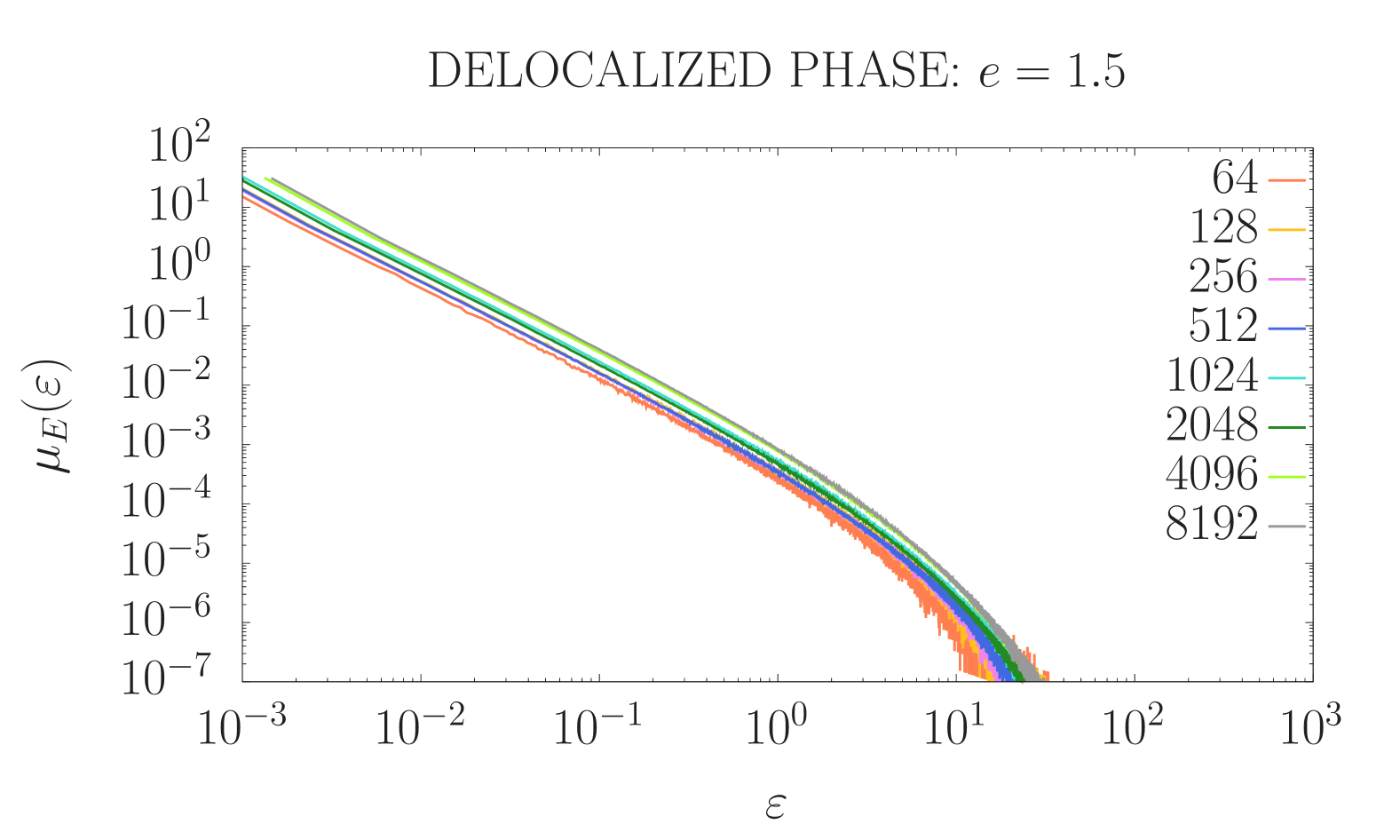
Figure 3: Marginal probability distribution of the local energy $\varepsilon_{j}=|z_{j}|^{4}$ for a single site of the lattice, averaged over all sites. System is in the homogeneous positive temperature phase: $E/N=1.5<e_{\textit{th}}$

.

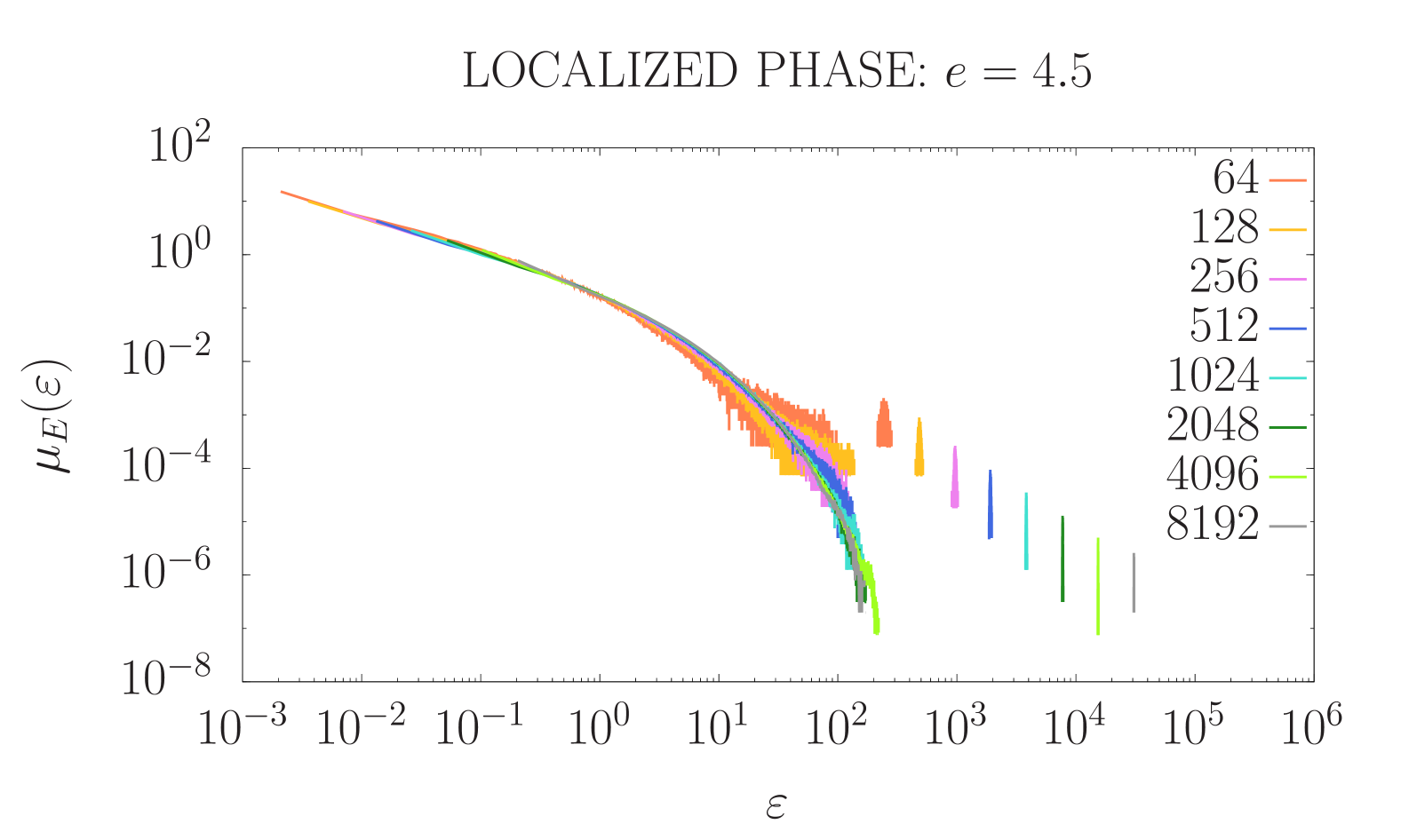
Figure 4: Marginal probability distribution of the local energy $\varepsilon_{j}=|z_{j}|^{4}$ for a single site of the lattice, averaged over all sites. System is in the localized negative temperature phase: $E/N=4.5>e_{c}$. Secondary peaks represent the characteristic condensate bump

.

IV.1 Entanglement: Numerical Results

Here are presented the numerical results for the measure of entanglement entropy in the delocalized and localized phase of the DNLSE. Since localization takes place for energy, we consider for the measure of entanglement the local energies $\varepsilon_{j}=|z_{j}|^{4}$. We are therefore led to consider the joint probability distribution $\varrho_{E}(\varepsilon_{1},\ldots,\varepsilon_{N})$, whose exact analytical expression is provided in Eq. (59) of [6]. The subscript $E$ explicitly indicates that the properties and shape of this distribution depend on the total energy $E$. We then define the marginal distribution for a single site of the DNLSE lattice:

$$\mu_{E}(\varepsilon_{j})=\text{Tr}_{\{\varepsilon_{i}\neq\varepsilon_{j}\}}[\varrho_{E}(\varepsilon_{1},\ldots,\varepsilon_{N})].$$ (16)

Since the choice of $\varepsilon_{j}$ is arbitrary, given that the lattice is homogeneous and we have periodic boundary conditions, we can drop the site index in the definition of Eq. (16): $\mu_{E}(\varepsilon_{j})=\mu_{E}(\varepsilon)$. While for the analytical estimate of $\mu_{E}(\varepsilon)$ we will use the formulae of [6], obtained from the large-deviation estimate of the microcanonical entropy, its numerical sampling is much simpler. Assuming the Hamiltonian dynamics of the DNLSE to be our importance sampling protocol for the microcanonical ensemble, the numerical estimate of $\mu_{E}(\varepsilon)$ is simply obtained by computing empirically $\mu_{E}(\varepsilon_{j})$ from the fluctuations along the dynamics and then averaging:

$$\mu_{E}(\varepsilon)=\frac{1}{N}\sum_{j=1}^{N}\mu_{E}(\varepsilon_{j})$$ (17)

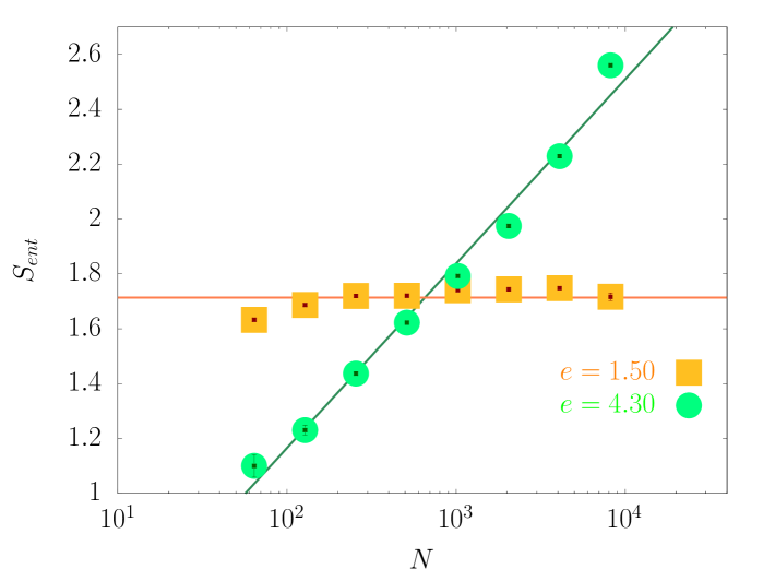
Figure 5: Behavior of the entanglement entropy $S_{\text{ent}}(N)$ measured numerically as a function of lattice size $N$. Orange squares: entanglement entropy of the homogeneous phase at positive temperature, $(e=1.5)<e_{th}$: Green circles: localized phase at negative temperature, $(e=4.5)>e_{c}$. In the homogeneous phase $S_{\text{ent}}(N)$ is constant while in the localized phase it grows as $S_{\text{ent}}\sim\log(N)$, as emphasized by the straight line in the semi-log scale.

In Fig. 3 and Fig. 4 is shown the shape of $\mu_{E}(\varepsilon)$ computed numerically at different lattice sizes $N$, respectively for the homogeneous and the localized phase. In particular in Fig. 3 the marginal distribution $\mu_{E}(\varepsilon)$ is computed for $E/N=1.5<e_{\textit{th}}$, where the temperature is positive and localization is absent. In Fig. 4 are shown marginals sampled at $E/N=4.5>\varepsilon_{c}$, where temperature is negative and the distributions exhibit the characteristic condensate bump [21, 6, 22]. From the numerically sampled marginals we then obtained the numerical estimate of entanglement entropy by simply applying the definition:

$$S_{\text{ent}}(N)=-\sum_{\varepsilon\in[\varepsilon_{\text{min}},\varepsilon_{\text{max}}]}\mu_{E}(\varepsilon)\log\mu_{E}(\varepsilon),$$ (18)

where $[\varepsilon_{\text{min}},\varepsilon_{\text{max}}]$ is the interval of energies where numerical values were sampled. The behaviour with system size of the entanglement entropy $S_{\text{ent}}(N)$ in the homogeneous and in the localized regime, which is the main result of this paper, is represented in Fig. 5. As expected, in the homogeneous positive temperature phase, where the thermodynamics is standard, entanglement entropy does not depend on system size: it remains constant upon varying $N$, its value being an offset which can be set to zero without any loss of generality. On the contrary we find that in the localized phase entanglement entropy shows the characteristic behaviour

$$S_{\text{ent}}(N)\sim\log(N),$$ (19)

which is well known to be typical of one dimensional entangled systems [23, 24]. This is to our knowledge the first time such a result has been found for a classical system. In fact, despite the condensate wave-function $z_{j}$ is a field of quantum origin, in the DNLSE framework it is treated as a classical field obeying Hamiltonian dynamics and is perfectly described by classical ensembles. The presence of a nontrivial behavior of the entanglement entropy, in the context of the present discussion, can be perfectly understood as due to the lack of locality enforced by the breaking down of the canonical description of the system: a quite new and unexplored regime where classical statistical mechanics seems to capture a phenomenology so far believed to characterize only pure quantum systems [25, 23, 26, 27]. The logarithmic behavior $S_{\text{ent}}\sim\log(N)$ has also a quite simple interpretation in terms of localization: as long as we identify the number of microstates with the possible locations of the breather on the lattice, which is equal to the number $N$ of lattice sites, it is then natural to say that the entropy of the system is $\log(N)$.

IV.2 Entanglement: Large-deviations results

We show in this section that the numerical result for the entanglement entropy in the localized phase of the DNLSE, presented in Fig. 5, is consistent with the analytical predictions which can be drawn from the exact knowledge of the marginal distribution $\mu_{E}(\varepsilon)$ that we have from [6, 7], which reads as:

$$\mu_{E}(\varepsilon) =f(\varepsilon)\qquad\quad~\varepsilon\ll\Delta E$$ (20)

$$\mu_{E}(\varepsilon) =g_{E}(\varepsilon)\qquad\quad\varepsilon\sim\Delta E,$$

with

$$f(\varepsilon) =\frac{1}{\sqrt{\varepsilon}}\,\exp{\left(-\sqrt{\varepsilon}\right)}$$ (21)

$$g_{E}(\varepsilon) =\frac{1}{\sqrt{2\pi\sigma^{2}}N^{3/2}}\,\exp{\left\{-\frac{(\varepsilon-\Delta E)^{2}}{2N\sigma^{2}}\right\}}$$ (22)

and where $\Delta E=E-E_{\textit{th}}$ is the excess energy with respect to the ensemble equivalence threshold $E_{\text{th}}=Ne_{\textit{th}}$, the energy value corresponding to infinite-temperature line in the phase diagram of Fig. 1. The function $g_{E}(\varepsilon)$ represents the Gaussian peak associated to the presence of a breather collecting on a single lattice site a macroscopic portion of excess energy $\Delta E$. This Gaussian peak is the well-known condensate bump characterizing the bimodal shape of $\mu_{E}(\varepsilon)$ in the localized phase. In Fig. 6, which must be compared with the numerical results of Fig. 4, is reported the analytical estimate of $\mu_{E}(\varepsilon)$ at different values of $N$, where the lattice size influences the position and shape of the secondary peak, see the above Eq. (22), since we have $\Delta E=N(e-e_{\textit{th}})$. In particular, the distributions of Fig. 6 are those obtained for $e=4.5>e_{c}$. From the explicit analytical knowledge of $\mu_{E}(\varepsilon)$ in the localized phase, in particular of its explicit dependence on $N$, it is obtained an analytic estimate of the dependence on $N$ of the entanglement entropy by exploiting the definition

$$S_{\text{ent}}(N)=-\int_{0}^{Ne}d\varepsilon~\mu_{E}(\varepsilon)\log\left(\mu_{E}(\varepsilon)\right)$$ (23)

The result of the numerical integration of the analytical expression of $\mu_{E}(\varepsilon)\log\mu_{E}(\varepsilon)$ is shown in Fig. 7, where the asymptotic behaviour $S_{\text{ent}}(N)\sim\log(N)$ can be clearly appreciated.

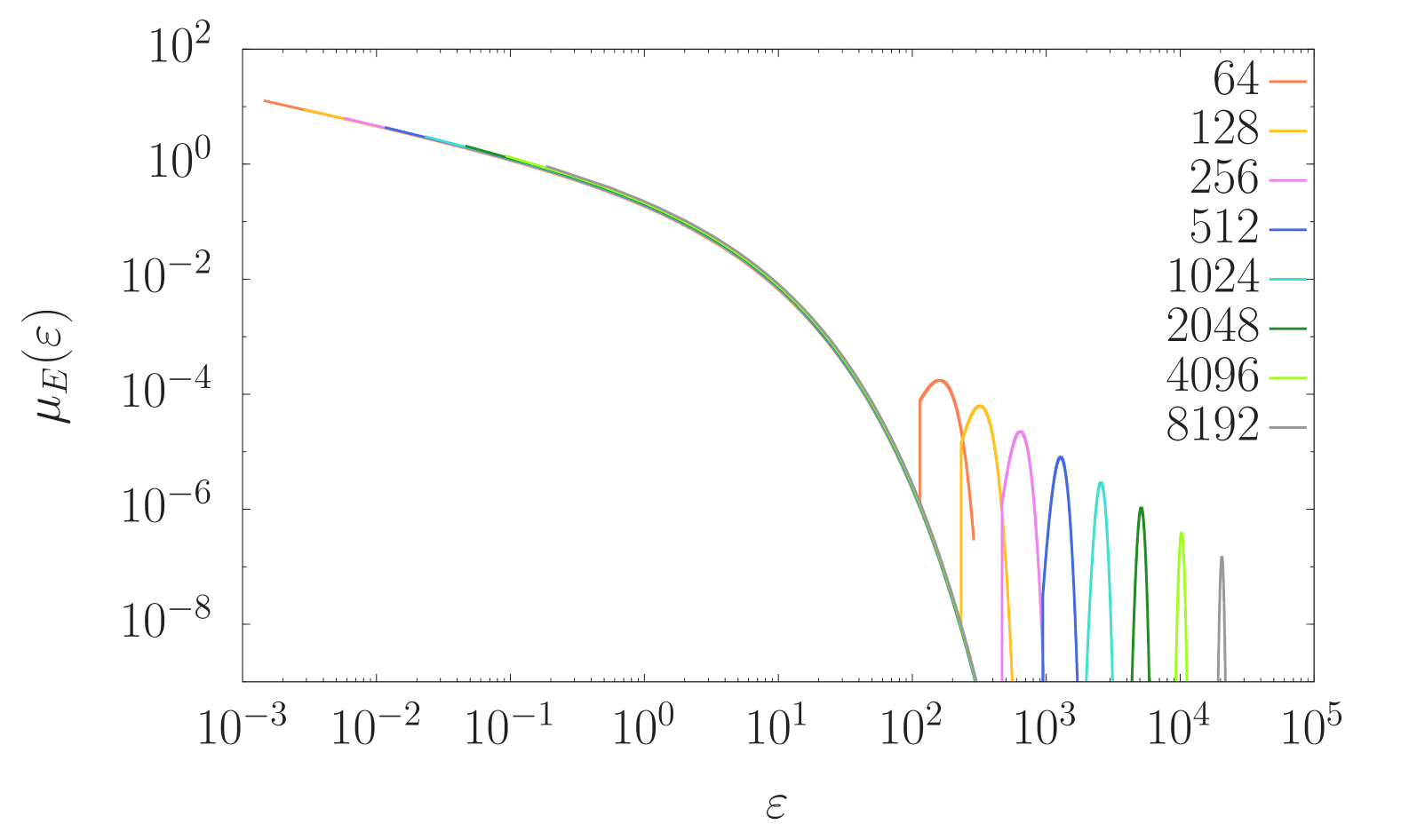
Figure 6: Analytical result for the marginal distribution $\mu_{E}(\varepsilon)$ at different values of the parameter $N$, see Eq. (22). The total energy is fixed to $E=Ne$, with $e=4.5>e_{c}$: the system is in the localized state.

Figure 7: Entanglement entropy computed from numerical integration of $\mu_{E}(\varepsilon)\log\mu_{E}(\varepsilon)$, where the expression of $\mu_{E}(\varepsilon)$ is the one of Eq. (22).

This result on entanglement entropy suggests a close analogy between the localized phase of the DNLSE and the properties associated to Many-Body Localization (MBL) in genuine quantum interacting systems [28, 29, 30]. In the DNLSE it is well known that, apart from the condensate total mass and energy, there are no exact conservation laws. An issue which fully deserves a deeper investigation, in the perspective of highlighting the analogies between this system and MBL, is therefore the search of an extensive number of quasi-conserved quantities also in the DNLSE, something which is here left for future investigations.

V Conclusions

In this work we have investigated numerically the thermodynamic properties of the localization transition in the Discrete Non-Linear Schrödinger Equation (DNLSE). Our results, which confirm the large-deviation analytical estimates of [6, 7], shed light on the controversial nature of the high energy localized phase of the DNLSE, which is now well established as an equilibrium phase in the microcanonical ensemble. We have then clarified how the correct definition of temperature in this phase can only be as a global observable in the microcanonical ensemble. Hamiltonian dynamics gave us validation of the equilibrium finite-size scaling predictions for the participation ratio and the negative temperature contained in [6, 7]. On the top of that, our most noticeable result is the behaviour of entanglement entropy in the localized phase, which grows as $S_{\text{ent}}(N)\sim\log(N)$. This result shed a light on the subtle and unexpected connection between classical and quantum systems. This is the first example of a field with classical statistics which exhibits a non-trivial behaviour of entanglement entropy, a fact related to the lack of statistical ensembles in the high energy phase. In this phase the global microcanonical constraint on energy cannot be released without having the disapparence of the localized phase itself. We have therefore ascertained that the localized phase of the DNLSE cannot be interpreted simply as a breather superimposed to an infinite temperature background [31, 32]: the whole system is entangled so that temperature makes sense as a physical observable only globally.

APPENDIX

App 1 Thermodynamic observables in the pseudo-localized phase

This section is dedicated to the study of the participation ratio and the microcanonical temperature for energies of the initial condition in the interval $e_{\text{th}}<e<e_{c}$, where the localized phase is metastable.

App 1.1 Participation ratio

In the regime $e_{\text{th}}<e<e_{c}$ we started dynamical simulations from either localized or homogeneous initial conditions. The corresponding data are reported in Fig. A1, where for comparison also the data points already discussed in the main text are shown with reference to Fig. 2 therein and relative to the homogeneous and localized phase. In Fig. A1 data points obtained from localized initial conditions, indicated as $loc$, are purple penthagons and red downward triangles, while those related to homogeneuos initial conditions are yellow triangles. The result is striking, in the sense that it really reveals the presence of two competing equilibrium phases. Starting from a localized state we find that even at moderately large $N$ the participation ratio $Y_{2}(N)$ relaxes to the equilibrium value of localized phase at $N=\infty$, that is $Y_{2}=(e-e_{\text{th}})^{2}/e^{2}$, marked by the corresponding horizontal line in the figure. We note that for all sizes $N$ considered in this intermediate regime, we have $e<e_{c}(N)$, so that the relaxation of $Y_{2}(N)$ to the value $Y_{2}(N=\infty)$ is an effect of the choice of initial conditions. In fact, at the very same energies, consider, for instance, the case $e=2.3$ in the figure, by initializing the Hamiltonian dynamics from a homogeneous initial condition, the system remains there, exhibiting a perfect homogeneous-phase scaling of the participation ration, $Y_{2}(N)\sim N^{-1}$. Elsewhere, this same regime was found to be characterized by persistent multibreather states [3] and by a nontrivial chaotic behavior [33, 34].

The sensible dependence on initial conditions in the regime $e_{\textit{th}}<e<e_{c}$ reveals the competing phase scenario typical of first-order like transitions. Even when the system is initialized in the metastable state, relaxation can be arbitrarily long, with a characteristic time scale growing exponentially fast with $N$ [35]. Concerning the dependence on $N$ of $Y_{2}(N)$ for energies in the intermediate regime $e_{\textit{th}}<e<e_{c}$, let us further comment Fig. A1 by noticing that the crossover of $Y_{2}(N)$ from the $1/N$ scaling to a constant value in the intermediate region is consistent, in particular for $e=2.25$ (red downwards triangles), with the same non-monotonic dependence on $N$ observed in [13, 14].

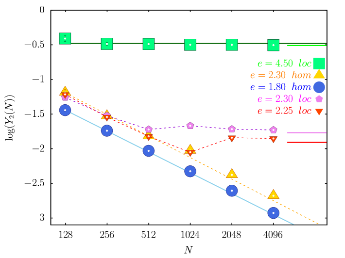
Figure A1: Finite-size scaling of the participation ratio $Y_{2}(N)$ of the DNLSE for $a=1$ and different energy densities $e$. Green squares: $e=4.5$, localized initial conditions ($loc$); Purple penthagons: $e=2.3$, localized initial conditions; red downward triangles: $e=2.25$, localized initial conditions; Yellow triangles: $e=2.3$, homogeneous initial conditions; Blue circles: $e=1.8$, homogeneous initial conditions. Statistical expectations are computed as time averages in the time interval $10^{5}$-$10^{6}$. Error bars are the standard deviation of fluctuations, sampled at intervals $\Delta t=10$, in the measurement window.

App 1.2 Negative temperature

For what concerns the finite-size scaling of temperature in the pseudo-localized regime, $e_{\text{th}}<e<e_{c}$, we find that the agreement with the analytical predictions of [6, 7]depends on the choice of initial conditions. As done for the participation ratio, in Fig. A2 we report both the data already shown in Fig. 2 of the main text, representing the negative temperature of the localized phase, and the data relative to the pseudo-localized phase. In this latter phase we find that for localized initial conditions the dependence of temperature on the system size $N$ seems to better agree with the analytical estimate $\beta\sim-N^{-1/3}$ given in [6] for the matching regime, while for homogeneous initial conditions it deviates more, in particular $\beta$ seems to decrease with $N$ sensibly slower than $N^{-1/3}$. We consider that the overall agreement between our numerical data on negative temperature in the pseudo-localized phase and analytical predictions is fairly good: in fact, it must be recalled that the behaviour $\beta\sim-N^{-1/3}$ is the one typical of the matching regime, that is energies in the neighbourhood of $e_{c}$, while the energy considered here, $e=2.3$, lies strictly below.
Furthermore, the dependence of the $\beta$-scaling with $N$ on the choice of initial conditions can be also intuitively explained in terms of the first-order like competing phases scenario, where a remarkably different behaviour can be found whether the system is initialized in the stable or metastable phase. And from this respect neither the localized nor the homogeneous initial conditions represent the true nature of the pseudo-localized phase, which is also characterized by large inhomogeneities in energy distribution across the chain. The difference between the pseudo-localized phase and the fully localized one is that in the former one the amount of energy $\varepsilon_{j}$ concentrated on a given site $j$ can still grow with $N$, but it cannot be proporional to it.

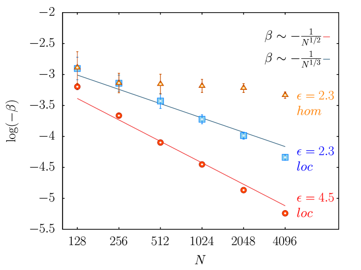
Figure A2: Finite-size scaling of minus the inverse temperature, $-\beta$, vs. $N$ in the metastable and stable localized phases. The system has been initialized with an artificial breather added to an infinite temperature background for the blue and red curves, and with a phase update algorithm for the orange curve. All systems are taken with $a=1$, while $e=4.5$ corresponds to the localized phase (red circles) and $e=2.3$ to the metastable phase (blue squares and orange triangles). The running time of the simulations is $\Delta\tau=1.5\times 10^{3}$ , and the microcanonical temperature has been measured globally across all the sites of the system. The uncertainties have been evaluated as the standard deviation of the temperature, measured at time intervals $d\tau=10$. The red and blue lines correspond to the theoretical exponents.

App 2 Non-locality of temperature

As outlined in the main text in Sec. III, the measure of a negative microcanonical temperature is a distinguishing feature of the localized phase: here we wish to present the evidence that it is precisely from the measure of temperature that we have a strong hint of the intrinsically non-local nature of the localized phase of the DNLSE and of its non-additive nature. In order to show this we performed the measure of $\beta_{\text{micro}}=\langle\mathcal{F}\{z_{j}\}\rangle_{E}$ by computing the function $\mathcal{F}$ only on sub-portions of the DNLSE lattice. The result is simple and at the same time striking: even if applying the correct microcanonical definition, any local measure of temperature yields a wrong result. Only if it happens that, by chance, the lattice portion containing the macroscopic breather is considered, the local measure of the temperature agrees with the global one. But in the thermodynamic limit the probability to end up in the system portion containing the breather is zero, so that it can be stated that, for any practical purpose, any local measurement of temperature is wrong. Data for local measures of microcanonical temperature in the DNLSE are shown in Fig. A3, in particular the temperature measured for 5 different portions of a $N=4096$ sites DNLSE lattice, each portion being made of $M=128$ sites. In Fig. A3 coloured continuous lines represent the temperatures of different lattice chunks, which are compared with the global temperature (black bullets). Data are sampled at $e=4.5>e_{c}(N)$: it can be clearly seen that in the localized phase local measures of the temperature do not agree with the global one. On the contrary, by doing the same comparison between global and local measures of temperature in the homogeneous “thermal” phase of the system (data for this case are not shown), $e<e_{\textit{th}}$, we have found agreement between the two measures of temperature, as can be expected from the equivalence between the canonical and microcanonical ensembles.

These results for temperature in the localized regime, $e>e_{c}(N)$, confirm that for the DNLSE in this particular phase the temperature $T$ cannot be traced back to a local quantity related to the average kinetic energy. This fact is not only a consequence of the lack of a standard kinetic-energy term in the DNLSE Hamiltonian, but is due to the nature of the localized phase, where $T$ is a function of all degrees of freedom (see, [19, 15]).

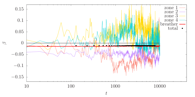
Figure A3: Local measurements of the inverse microcanonical temperature $\beta(t)=\mathcal{F}(\vec{x}(t))$ as a function of time $t$ for a lattice with $N=1024$ points, $a=1$ and energy $e=4.5$. Continuous lines: local value of $\beta$ measured for generic chunks of $M=100$ with no breather inside; Red triangles: local value of $\beta(t)$ measured for the chunk of $M=100$ with the breather inside; Black dots: global measurement of $\beta$ computed over all lattice sites.

App 3 Ergodicity breaking

Despite all results presented in the main text of this paper are focused on the DNLSE thermodynamics in the localized phase, dynamical properties of this system are also an extremely interesting chapter on its own. To maintain the discussion of this work self-contained we have decided to present just a brief account of the dynamical properties of the system in this section, leaving further investigations for a future work, as for instance the study of the similarities between the DNLSE localization transition and the ergodicity breaking transitions in disordered systems. It must be also acknowledged that the study of the DNLSE slow dynamics, apart from comparisons with the dynamics of glassy systems, has already attracted a lot of interest, with many interesting works already dedicated to this specific subject [33, 35].

For what concerns the present discussion we just want to present a hint that, consistently with the most naive expectation, localization corresponds to a form of ergodicity breaking. The evidence of this is provided by the behavior of time correlation functions $C(t,t_{w})$, for which numerical data are shown in Fig. A4. Since the variable of interest throughout the whole discussion in this work is the non-linear contribution to local energy of the condensate wave-function, $\varepsilon_{i}(t)=|z_{i}(t)|^{4}$, we have considered the following definition for the two-time correlation function:

$$C(t,t_{w})=\frac{1}{\mathcal{Z}(t_{w})}\sum_{i=1}^{N}\varepsilon_{i}(t)\varepsilon_{i}(t_{w}),$$ (A1)

where $\mathcal{Z}(t_{w})=\sum_{i=1}^{N}\varepsilon_{i}^{2}(t_{w})$ provides the correct normalization. The naive expectation that the pseudo-localized, $e_{\text{th}}<e<e_{c}$, and localized, $e>e_{c}$, regimes are also ergodicity-broken phases seems confirmed from a first analysis of the correlation function $C(t,t_{w})$, in which we have kept for full generality the dependence on both initial, $t_{w}$, and final, $t$, time. We have denoted the initial time $t_{w}$ in order to stress the analogy with the waiting time of glass-forming systems. When the system is initialized with a finite fraction of the total energy localized in a single breather, data in Fig. A4 show that, up to $t=3.0\cdot 10^{4}$ correlations either never decay in the localized phase, $e=4.5>e_{c}$, or decay to a plateau at $C^{*}\sim 0.75$ in the pseudo-localized one, $e=2.3$. We also studied how initial data evolve at energies $e<e_{\text{th}}$ where there is no localization, temperature is positive and equivalence between canonical and microcanonical ensemble holds. In particular, we have studied how correlations decay for an initial condition at $e=1.8<e_{\text{th}}$: we find that initial conditions with a finite fraction of energy on a single lattice site decay to $1\%$ of the initial value within times $t=3.0\cdot 10^{4}$, whereas homogeneous initial conditions at the same energy decay exponentially fast. These data do not allow us to determine the specific type of ergodicity breaking transition observed or to characterized the aging dynamics at work. They just provide the evidence that localization is accompanied by a dynamical arrest, encouraging to further investigations in this direction.

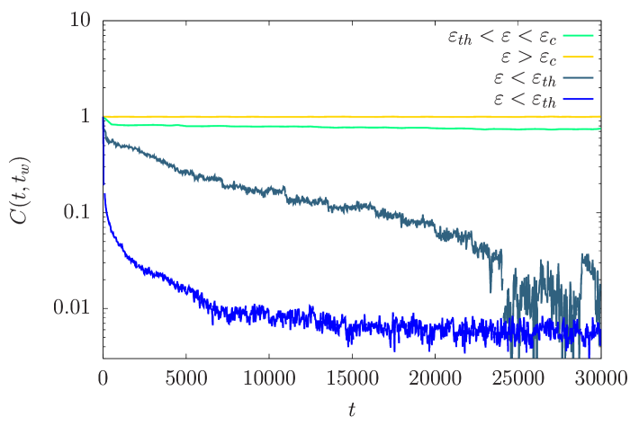
Figure A4: Time correlation function $C(t,t_{w})$ for a $N=1024$ DNLSE lattice at different values of energy and for different initial conditions. Energy values: $e=4.5>e_{c}$, negative temperature localized phase (yellow line); $e_{\text{th}}<e=2.3<e_{c}$, negative temperature pseudo-localized phase (green line); $e=1.8<e_{\text{th}}$, positive temperature homogeneous phase. For the homogeneous phase, $e<e_{\text{th}}$, we have considered both localized (gray line) and homogeneous (blue line) initial conditions. The curves have been obtained by averaging over independent initial conditions (10 for $e>e_{c}$, 100 for $e_{\text{th}}<e<e_{c}$, 50 for $e<e_{\text{th}}$ localized initial conditions, 500 for $e<e_{\text{th}}$ homogeneous initial conditions).

App 4 Microcanonical Temperature

An operative definition of microcanonical temperature $T^{-1}=\partial S/\partial E$ is obtained following the results in [15], where the cartesian real coordinates $x_{2j}=q_{j}\equiv\sqrt{2}~\text{Im}(z_{j})$, $x_{2j+1}=p_{j}\equiv\sqrt{2}~\text{Re}(z_{j})$ are introduced, so that

$$\vec{x}=\{p_{1},q_{1},p_{2},q_{2},\ldots,p_{N},q_{N}\}.$$ (A2)

In this representation the energy and total mass appearing in Eq.(4) and Eq. (5) can be written as

$$\mathcal{H} = \sum_{j=1}^{N}\frac{1}{4}(p_{j}^{2}+q_{j}^{2})^{2}+\sum_{j=1}^{N}(p_{j}p_{j+1}+q_{j}q_{j+1})$$ (A3)

$$\mathcal{A} = \frac{1}{2}\sum_{j=1}^{N}(p_{j}^{2}+q_{j}^{2}),$$ (A4)

or, equivalently, as

$$\mathcal{H} = \sum_{j=1}^{N}\frac{1}{4}(x_{2j}^{2}+x_{2j+1}^{2})^{2}+\sum_{j=1}^{N}(x_{2j+1}x_{2j+3}+x_{2j}x_{2j+2})$$

$$\mathcal{A} = \frac{1}{2}\sum_{j=1}^{2N}x_{j}^{2}.$$ (A5)

In terms of these variables one can then write the global function $\mathcal{F}(\vec{x})$ such that $\beta=T^{-1}=\langle\mathcal{F}(\vec{x})\rangle_{E}$ as

$$\mathcal{F}(\vec{x})=\frac{W(\vec{x})\|\vec{\xi}\|}{\vec{\nabla}\mathcal{H}\cdot\vec{\xi}}\ \vec{\nabla}\cdot\left(\frac{\vec{\xi}}{W(\vec{x})\|\vec{\xi}\|}\right)$$ (A6)

where the vector $\vec{\xi}$ and the function $W(\vec{x})$ are defined as

$$\vec{\xi} = \frac{\vec{\nabla}\mathcal{H}}{\|\vec{\nabla}\mathcal{H}\|}-\frac{(\vec{\nabla}\mathcal{H}\cdot\vec{\nabla}\mathcal{A})\vec{\nabla}\mathcal{A}}{\|\vec{\nabla}\mathcal{H}\|\|\vec{\nabla}\mathcal{A}\|^{2}}$$ (A7)

$$W(\vec{x}) = \sqrt{\sum_{\genfrac{}{}{0.0pt}{}{j,k=1}{j<k}}^{2N}\left[\frac{\partial\mathcal{H}}{\partial x_{j}}\frac{\partial\mathcal{A}}{\partial x_{k}}-\frac{\partial\mathcal{H}}{\partial x_{k}}\frac{\partial\mathcal{A}}{\partial x_{j}}\right]^{2}}\,.$$

Notice that the resulting definition Eq. (A6) is nonlocal in space, as it involves the contribution of all degrees of freedom.

References

- Kevrekidis [2009] P. G. Kevrekidis, The Discrete Nonlinear Schrödinger Equation (Springer Verlag, Berlin, 2009).
- Rasmussen et al. [2000] K. O. Rasmussen, T. Cretegny, P. G. Kevrekidis, and N. Grønbech-Jensen, Phys. Rev. Lett. 84, 3740 (2000).
- Iubini et al. [2013] S. Iubini, R. Franzosi, R. Livi, G.-L. Oppo, and A. Politi, New Journal of Physics 15, 023032 (2013).
- Baldovin et al. [2021] M. Baldovin, S. Iubini, R. Livi, and A. Vulpiani, Physics Reports 923, 1 (2021).
- Iubini and Politi [2025] S. Iubini and A. Politi, Phys. Rev. Lett. 134, 097102 (2025).
- Gradenigo et al. [2021a] G. Gradenigo, S. Iubini, R. Livi, and S. N. Majumdar, Journal of Statistical Mechanics: Theory and Experiment 2021, 023201 (2021a).
- Gradenigo et al. [2021b] G. Gradenigo, S. Iubini, R. Livi, and S. N. Majumdar, The European Physical Journal E 44, 1 (2021b).
- Campa et al. [2009] A. Campa, T. Dauxois, and S. Ruffo, Physics Reports 480, 57 (2009).
- Ruelle [1969] D. Ruelle, Statistical Mechanics, Rigorous Results (W.A. Benjamin, 1969).
- Arezzo et al. [2022] C. Arezzo, F. Balducci, R. Piergallini, A. Scardicchio, and C. Vanoni, Journal of Statistical Physics 186, 1 (2022).
- Yoshida [1990] H. Yoshida, Physics letters A 150, 262 (1990).
- Boreux et al. [2010] J. Boreux, T. Carletti, and C. Hubaux, arXiv preprint arXiv:1012.3242 (2010).
- Gotti et al. [2021] G. Gotti, S. Iubini, and P. Politi, Physical Review E 103, 052133 (2021).
- Gotti et al. [2024] G. Gotti, S. Iubini, and P. Politi, Fluctuation and Noise Letters 23, 2440007 (2024).
- Franzosi [2011] R. Franzosi, Journal of Statistical Physics 143, 824 (2011).
- Iubini et al. [2012] S. Iubini, S. Lepri, and A. Politi, Physical Review E—Statistical, Nonlinear, and Soft Matter Physics 86, 011108 (2012).
- Levy and Silberberg [2018] U. Levy and Y. Silberberg, Physical Review B 98, 060303 (2018).
- Levy [2021] U. Levy, in Progress in Optics, Vol. 66 (Elsevier, 2021) pp. 131–170.
- Rugh [1997] H. H. Rugh, Physical Review Letters 78, 772 (1997).
- Henderson and Vedral [2001] L. Henderson and V. Vedral, Journal of Physics A: Mathematical and General 34, 6899 (2001).
- Majumdar et al. [2005] S. N. Majumdar, M. Evans, and R. Zia, Physical review letters 94, 180601 (2005).
- Mori et al. [2021] F. Mori, G. Gradenigo, and S. N. Majumdar, Journal of Statistical Mechanics: Theory and Experiment 2021, 103208 (2021).
- Calabrese and Cardy [2005] P. Calabrese and J. L. Cardy, J. Stat. Mech. 0504, P04010 (2005), arXiv:cond-mat/0503393 .
- Nezhadhaghighi and Rajabpour [2013] M. G. Nezhadhaghighi and M. A. Rajabpour, Physical Review B 88, 10.1103/physrevb.88.045426 (2013).
- Calabrese and Cardy [2004] P. Calabrese and J. L. Cardy, J. Stat. Mech. 0406, P06002 (2004), arXiv:hep-th/0405152 .
- Calabrese and Cardy [2009] P. Calabrese and J. Cardy, J. Phys. A 42, 504005 (2009), arXiv:0905.4013 [cond-mat.stat-mech] .
- Eisert et al. [2010] J. Eisert, M. Cramer, and M. B. Plenio, Rev. Mod. Phys. 82, 277 (2010).
- Nandkishore and Huse [2015] R. Nandkishore and D. A. Huse, Ann. Rev. Condensed Matter Phys. 6, 15 (2015), arXiv:1404.0686 [cond-mat.stat-mech] .
- Abanin et al. [2019] D. A. Abanin, E. Altman, I. Bloch, and M. Serbyn, Rev. Mod. Phys. 91, 021001 (2019), arXiv:1804.11065 [cond-mat.dis-nn] .
- Laflorencie [2016] N. Laflorencie, Phys. Rept. 646, 1 (2016), arXiv:1512.03388 [cond-mat.str-el] .
- Rumpf [2004] B. Rumpf, Phys. Rev. E 69, 016618 (2004).
- Rumpf [2009] B. Rumpf, Physica D: Nonlinear Phenomena 238, 2067 (2009).
- Mithun et al. [2018] T. Mithun, Y. Kati, C. Danieli, and S. Flach, Physical Review Letters 120, 184101 (2018).
- Iubini and Politi [2021] S. Iubini and A. Politi, Chaos, Solitons & Fractals 147, 110954 (2021).
- Iubini et al. [2019] S. Iubini, L. Chirondojan, G.-L. Oppo, A. Politi, and P. Politi, Physical review letters 122, 084102 (2019).