Confidence Intervals Using Turing’s Estimator: Simulations and Applications
Abstract
Turing’s estimator allows one to estimate the probabilities of outcomes that either do not appear or only rarely appear in a given random sample. We perform a simulation study to understand the finite sample performance of several related confidence intervals (CIs) and introduce an approach for selecting the appropriate CI for a given sample. We give an application to the problem of authorship attribution and apply it to a dataset comprised of tweets from users on X (Twitter). Further, we derive several theoretical results about asymptotic normality and asymptotic Poissonity of Turing’s estimator for two important discrete distributions.
Keywords: Turing’s estimator; Good-Turing estimation; authorship attribution; confidence intervals.
1 Introduction
Turing’s estimator allows one to estimate the probabilities of outcomes that appear only rarely in a random sample. This includes ones that do not appear in the sample at all (the missing mass) and ones that appear exactly times for some relatively small (the th occupancy probability). We are focused on applications to linguistics, where outcomes are words used by an author. In other applications, outcomes may be species in an ecosystem (Chao et al. (2015)), anatomical locations of metastatic tumors (Newton et al. (2014)), expressed sequence tags (ESTs) for genetic identification (Lijoi et al. (2007)), word trigrams for speech recognition (Gupta et al. (1992)), colors of balls in an urn (Decrouez et al. (2016)), or different fortunes placed into fortune cookies (Gou et al. (2024)). To abstract away from any concrete application, we typically describe outcomes as letters in some finite or countably infinite alphabet.
Turing’s estimator is also sometimes called Turing’s formula or the Good-Turing estimator. It was first published by I.J. Good in Good (1953), where the idea was largely credited to Alan Turing. Turing had developed it while working to break the Enigma code during World War II, see Good (2000) for a discussion of its application in this context. There has been much work on understanding the statistical properties of Turing’s estimator. This includes studies of its bias and mean squared error (MSE) (Robbins (1968); Chao et al. (1988); Grabchak & Cosme (2017); Painsky (2023); Pananjady et al. (2024)), its consistency (Ohannessian & Dahleh (2012)), and its asymptotic distributions (Esty (1982); Esty (1983); Zhang & Huang (2008); Zhang & Zhang (2009); Zhang (2013); Grabchak & Zhang (2017); Chang & Grabchak (2023)). See also the monograph Zhang (2017) for a detailed overview. The asymptotic distributions of Turing’s estimator allow one to develop confidence intervals (CIs) for the missing mass and for the occupancy probabilities. However, different situations can lead to different limiting distributions and thus to a number of different CIs.
The goals of this paper are threefold. The first is to understand the finite sample performance of the various CIs and to find a way to choose the appropriate CI for a given dataset. The second is to develop a novel methodology for using these CIs for the problem of authorship attribution. The third is to theoretically verify when asymptotic normality and asymptotic Poissonity hold for Turing’s estimator when sampling from discrete uniform and geometric distributions. This is important since currently available sufficient conditions are fairly complicated and verifying them in concrete situations is not trivial.
The rest of this paper is organized as follows. In Section 2, we formally present Turing’s estimator, review the various asymptotic results available in the literature, and convert them to CIs. We also introduce the so-called Heuristic CI, which alternates between the others depending on the properties of a given random sample. In Section 3, we give our simulation results with a focus on three classes of distributions: discrete uniform, geometric, and discrete Pareto. To give the simulations more context, we also present our theoretical results here. In Section 4, we develop a novel methodology for authorship attribution and apply it to a dataset comprised of tweets from users on X (Twitter). The goal is to check if two X accounts are from the same author, which is important for the problem of identifying fake accounts. A summary along with a discussion is given in Section 5. Appendix A summarizes the known sufficient conditions for asymptotic normality and asymptotic Poissonity of Turing’s estimator and Appendix B presents the proofs of our theoretical results.
2 Confidence Intervals for Occupancy Probabilities
Let be a finite or countably infinite set. We refer to as the alphabet and to the elements in as letters. Let , with and for each , be a probability distribution on . In practice, we do not know the distribution , which must be estimated from data. Let be a random sample of size on the alphabet with distribution . For each , let be the number of times that letter appears in the sample. For , define
Here, is the conditional probability (given the sample) of seeing a letter that appears exactly times in the sample and is the number of letters that appear exactly times. We refer to as the th occupancy probability and to as the th occupancy count. When , the quantity is also called the missing mass. It is the probability of seeing a letter that has not been seen before. The quantity is called the coverage of the random sample. When this quantity is small, the sample is not representative and does not provide much information about the underlying distribution; see Zhang & Grabchak (2013) for a discussion.
For the th order Turing’s estimator is an estimator of given by
The bias of this estimator is given by
| (1) |
The asymptotic standard deviation of can be given by
| (2) |
and it can be estimated by
see Chang & Grabchak (2023) for details.
A number of asymptotic confidence intervals (CIs) for have been proposed in the literature. These are based on various limit theorems. If , then, under mild conditions (see Appendix A), we have
| (3) |
and
| (4) |
These lead to the CIs given, respectively, by
| (5) |
and
| (6) |
where denotes the quantile of the standard normal distribution. For the CI in (5), we take the lower bound to be when and the upper bound to be when . Further, we take the CI to be the point estimator when . For the CI in (6), we take it to be the point estimator when and we take the upper bound to be when . Note that the lower bound cannot be negative in this case. We refer to the CI in (5) as the Normal CI and to the one in (6) as the Normal Ratio CI. The Normal CI was first given for in Zhang & Huang (2008) and it was extended to in Zhang (2013), see also Zhang & Zhang (2009) and Chang & Grabchak (2023). We have not seen the Normal Ratio CI written out before. However, the theory was developed in Grabchak & Zhang (2017) and Chang & Grabchak (2023).
If , then, under mild conditions (see Appendix A), we have asymptotic Poissonity, i.e., a Poisson distribution in the limit. In this case, for , we have
| (7) |
where denotes a Poisson distribution with mean . There are many approaches for deriving a CI for the mean of a Poisson distribution; see, e.g., the survey paper Sahai & Khurshid (1993) and the references therein. We follow a standard approach based on a chi-squared approximation, which can be found in Section 4.7.3 of Johnson et al. (2005). The resulting CI for is given by
| (8) |
where denotes the quantile of the chi-squared distribution with degrees of freedom. When , we take this interval to be . Thus, this CI never degenerates to a point. We refer to the CI in (8) as the Poisson CI. We have not seen this CI written out before. However, the theory was derived in Theorem 2 of Zhang & Zhang (2009) for and Theorem 2.3 in Chang & Grabchak (2023) for . We note that for , a similar CI for the related quantity is given in Esty (1982).
From a theoretical perspective, the CIs based on asymptotic normality should work better when and the one based on asymptotic Poissonity should work better when . In practice, of course, we do not know the asymptotics of . However, we can estimate by , which suggests the following heuristic for choosing between the two types of CIs. First, select a threshold . If , use (8), otherwise use (5) or (6). We call this the heuristic CI. Here, is a tuning parameter.
We now discuss several variants of the above CIs that appear in the literature. Perhaps the most prominent is the CI introduced in Esty (1983). While there it was only given for , it can be formulated for any by
| (9) |
While, asymptotically, it is equivalent to the CI in (5), for any finite this CI is narrower. In a different direction, all of the CIs discussed above can be constructed using a modified version of Turing’s estimator. This version is used in, e.g., Zhang (2013) and Grabchak & Zhang (2017). It is given by
The bias of this estimator is as in (1), but with in place of . Asymptotically there is no difference between the two. All of the CIs discussed above can be modified to use in place of . We note that is the form that was originally introduced in Good (1953).
3 Simulations
We performed a series of simulations to better understand the performance of the various CIs discussed in Section 2. In the interest of space, we only give detailed results for three CIs. These are the Normal CI given in (5), the Poisson CI given in (8), and a version of the Heuristic CI with tuning parameter . Here, the Heuristic CI chooses the Poisson CI when and otherwise it chooses the Normal CI. We tried a variety of choices for , but seemed to work best. We leave the question of how to optimize the choice of for future work.
While we do not give detailed results for the other CIs, we performed many simulations with them and now give a brief summary. We found that there is essentially no difference in using CIs based on the modified Turing’s estimator in place of , even for small sample sizes. When comparing the CI in (9) with the Normal CI, we observed that the Normal CI was typically a little wider, but had better coverage, sometimes significantly so. The Normal Ratio CI given in (6) had comparable performance to the Normal CI in most situations. Sometimes it performed a little better and sometimes a little worse. The problem is that sometimes the method would essentially fail. This seems to be related to the situations where and the upper bound in the CI is replaced by .
We now present our detailed simulation results. These focus on the Normal CI, the Poisson CI, and the Heuristic CI in the context of three families of distributions.
Discrete Uniform Distribution
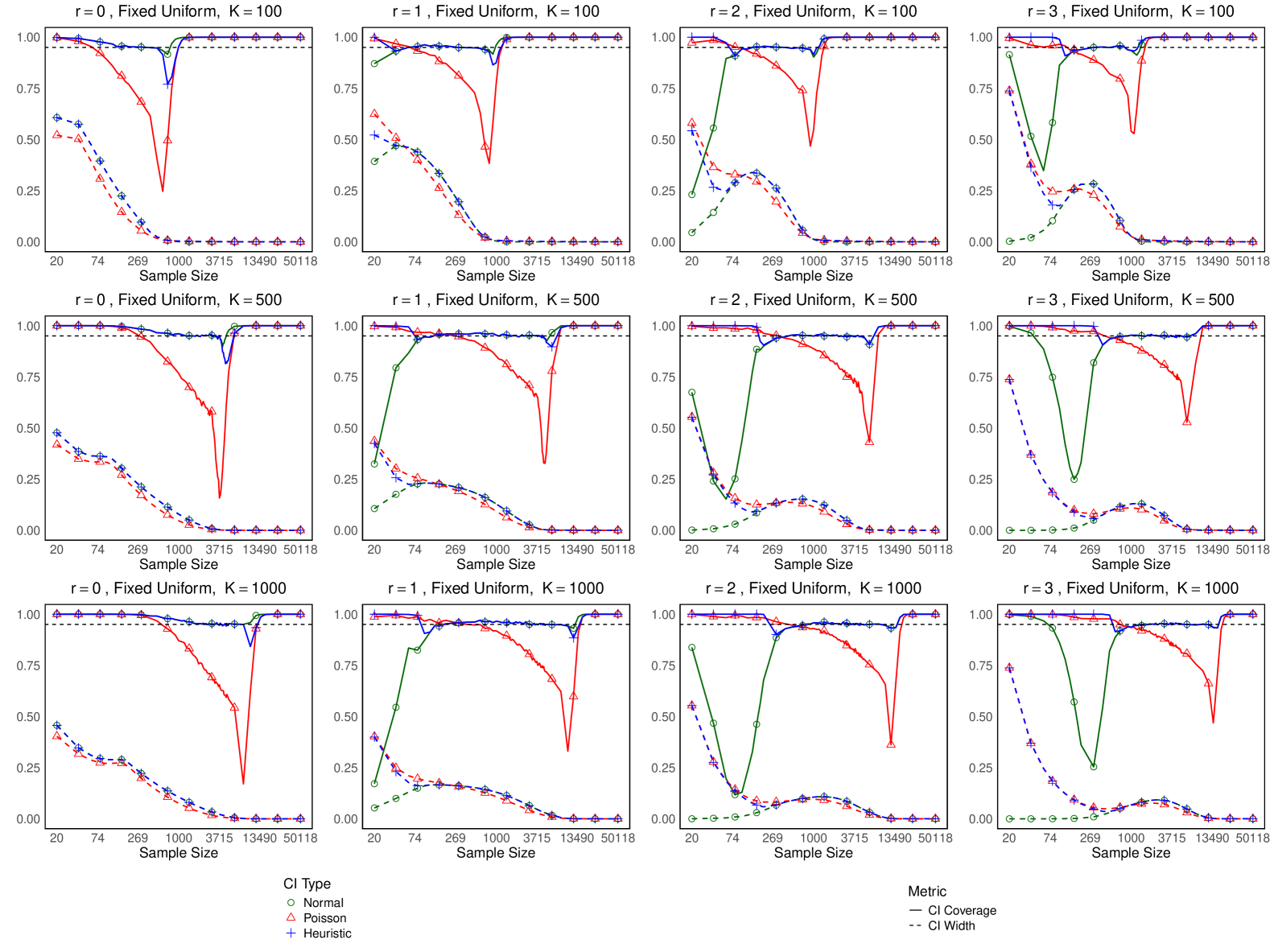
The discrete uniform distribution has a probability mass function (pmf) given by
| (10) |
where integer is a parameter. It is easily checked that
as . Thus, the known sufficient conditions needed for the asymptotics underpinning the various CIs do not hold. Nevertheless, our simulation results suggest that the CIs generally work well.
For the simulations, we considered three choices of and a variety of sample sizes . For each choice of and , we simulated samples (replications). For each sample and each , we constructed the Normal CI, the Poisson CI, and the Heuristic CI, each at the confidence level. We then found the coverage proportion, i.e., the proportion of the time that each CI contained the true value , and we calculated the sample means of the widths of the CIs. This information is summarized in Figure 1. We can see that the Normal CI and the Heuristic CI have very good performance, with the Poisson CI typically performing worse. While there are some cases where the Poisson CI outperforms the Normal CI in terms of coverage, this is at the expense of wider, often significantly wider, CIs. The Heuristic CI always has the best performance in terms of coverage and its width is never wider than the largest width of the other two.
It may be interesting to note that the proportion of CIs containing the true value does not converge to , but to . This cannot be explained through having wide CIs, as the widths are very close to when this happens. The explanation is that the discrete uniform distribution has only a finite number of possible values and, for large enough , we are likely to see all letters multiple times. This would lead us to have , , and . In this case the Normal CI will become the singleton and any interval that contains will contain . A similar situation holds for the Poisson CI.
What may be even more interesting is that the coverage of the Normal CI appears to converge to for large, but not too large, values of the sample size . Such apparent convergence before the actual convergence is sometimes called pre-limit behavior, see Grabchak & Samorodnitsky (2010) and the references therein for a discussion in a somewhat different context. The theoretical explanation for this pre-limiting, apparent convergence is the fact that, while the limits in (3), (4), and (7) do not hold for any fixed value of , they can hold when increases with the sample size. Specifically, assume that, for sample size , the parameter is given by , where and is the floor function. In this case, we have a sequence of discrete uniform distributions with pmfs of the form
| (11) |
for some that does not depend on . Thus, the distribution is changing dynamically with the sample size, and we refer to it as the dynamic discrete uniform. In this context, we refer to the distribution given in (10) as the fixed discrete uniform distribution. Note that the larger the value of , the faster the number of letters in the distribution grows. When discussing dynamic distributions, we take to be as given by (2), but with in place of .
We derive asymptotic theory for the dynamic discrete uniform in Appendix B.1. The results can be summarized as follows:
-
1.
For and and for , , and , we have asymptotic normality.
-
2.
For , , and , we have asymptotic Poissonity with mean .
-
3.
For , , and , we have with .
-
4.
For , we have with .
-
5.
Current state-of-the-art asymptotic results cannot tell us what happens when and or when and . However, we do know that in these cases.
Recall that is the asymptotic standard deviation of . Thus, means that there is either no asymptotic distribution or that the rate of convergence is strictly slower than . Note that for we have both when is small () and when it is large (). This seems to be for opposite reasons. When is small, the number of letters grows slowly as compared to the sample size, and for large samples we are likely to have observed all of the letters more than times. On the other hand, when is large, the number of letters grows quickly, and for large samples we are unlikely to have seen any letter or more times.
In the context of the fixed discrete uniform distribution, the asymptotic results suggest the following. Assume that the parameter in (10) is relatively large. If for some values of and we have asymptotic normality in the dynamic case, then for (large) sample sizes that are on the order of , we should be close to normal and the normal CI should work well. However, for sample sizes that are much larger than , we should no longer be close to normal. A similar result should hold for asymptotic Poissonity. Note that for , asymptotic Poissonity holds for larger values of (smaller values of ) than the values where asymptotic normality holds. Thus, we would expect the Poisson CI to work well for large (but not too large) sample sizes, then for even larger sample sizes we would expect the Normal CI to work well, and for very large sample sizes everything should approach by the arguments given previously. This is very much in keeping with what we see in Figure 1.
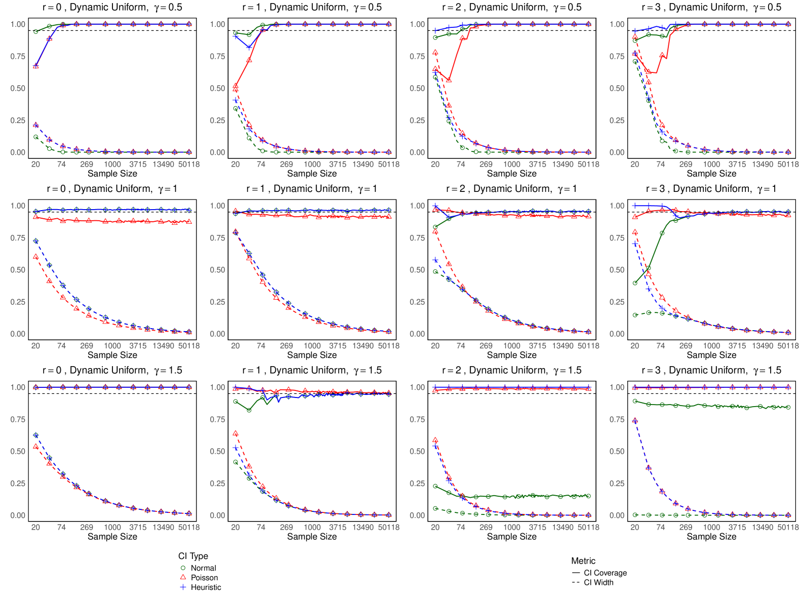
To better understand the dynamic situation, we performed a simulation study for this case. The results are given in Figure 2. The simulations were performed in a similar manner to the fixed discrete uniform case, except that now, instead of fixing , we fix and then choose dynamically depending on . We can see that the Heuristic CI again has the best performance in terms of coverage. However, its performance is slightly worse than the Normal CI for small sample sizes when and .
Based on the theoretical results, we have asymptotic normality when , and when , . In these cases, we can see that, for larger sample sizes, the normal CI is close to the line. It should be noted that the Poisson CI also performs well here. This may be related to the fact that the normal distribution provides a good approximation to a Poisson distribution when the mean is large, but this requires further study. We have asymptotic Poissonity when and . We can see that the Poisson CI works well in this case, while the Normal CI has very poor performance. In this case, the mean of the asymptotic Poisson distribution is and the normal approximation to the Poisson will not work well.
We now turn to the situations where . For we can observe that all three CIs converge to and that the widths get very close to . This is in keeping with what we saw for the fixed discrete uniform and seems to be for similar reasons. The situation seems to be very different when and . Here, the Poisson CI has very high coverage, but the Normal CI does not. However, we conjecture that this situation should actually be similar to that of , but that we would need much larger sample sizes to see this. Our justification is that, in this case, at a much slower rate. To check this conjecture we would need to perform simulations with much larger sample sizes. Due to computational constraints, we are only able to obtain preliminary results. For sample sizes and , we simulated replications. The results are summarized in Table 1. We can see that the coverage of the Normal CI does seem to approach , but this requires further study. We note that, in all of these simulations, we observed .
| CI | Coverage | Mean Width | |
|---|---|---|---|
| Normal | 82/100 | ||
| Poisson | 100/100 | ||
| Heuristic | 100/100 | ||
| Normal | 93/100 | 0 | |
| Poisson | 100/100 | ||
| Heuristic | 100/100 |
We conclude this discussion by considering the situations for which theoretical results are not known. For and , all three CIs seem to perform well, and they essentially give coverage, although with fairly wide CIs. These results do not suggest that asymptotic normality or asymptotic Poissonity hold, but they do not preclude it either. On the other hand, when and , the situations look very much like what we would expect if asymptotic normality held. We leave the problem of verifying this theoretically as an important direction for future work.
Geometric Distribution
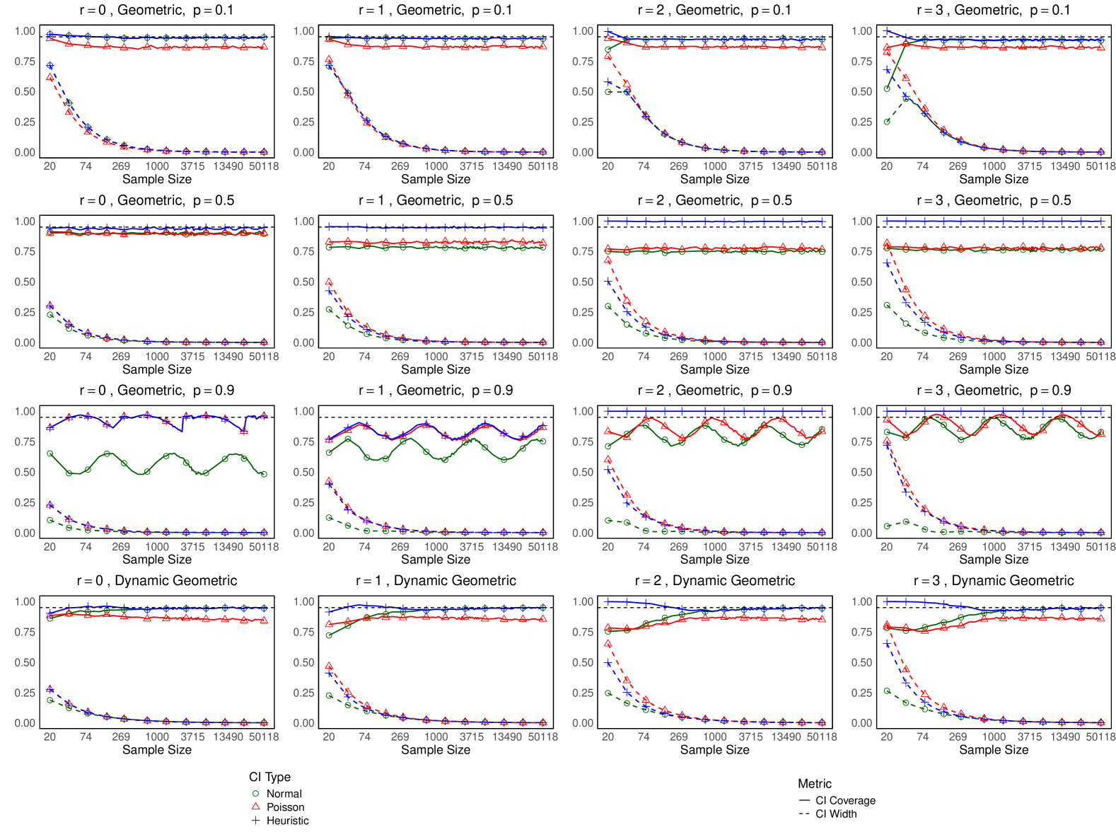
The geometric distribution has a pmf given by
| (12) |
where is a parameter. The following is an immediate consequence of the slightly more general Proposition 2 given below.
Proposition 1.
Let . We have
| (13) |
This means that the known sufficient conditions for (3) and (4) do not hold. It is not known if exists. However, known results about a related quantity lead us to conjecture that it does not, see Theorem 3 in Zhang (2018). Even if it does exist, the known sufficient conditions for (7) do not hold, see the discussion just below Theorem 2.3 in Chang & Grabchak (2023).
The simulations were performed in a similar manner to those for the discrete uniform distribution. We considered the parameter values: . The results are summarized in the first three rows of Figure 3. We can see that the widths converge to , but that the coverage proportions do not approach . Instead, they appear to be either constant or, in the case of , they seem to oscillate around a fixed value. It may be interesting to note that, in the situations where they oscillate, they seem to do so with a period that appears constant on a log scale. We do not know why this is, but it suggests an interesting direction for future work.
In all cases, the Heuristic CI seems to work very well. We can see two situations. In the first, the Heuristic CI pretty much always selects one method. This happens when with and when with . In all of these cases, the method that is selected is the best performing one. It should be noted that this best method is not always the same. Specifically, it is the Normal CI when and the Poisson CI when .
The other situation, which happens in all of the remaining cases, sees the Heuristic CI significantly outperform the other two. For instance, when and , the Normal and Poisson CIs each have about coverage, while the Heuristic CI is close to . Clearly, in these cases, the Heuristic CI alternates between the other two, selecting the better CI for the given simulation.
Even though we do not have asymptotic normality or asymptotic Poissonity, we can see that for , the Normal CI seems to be close to . This can, again, be explained by considering a dynamic situation, where the distribution changes with the sample size. Specifically, assume that the parameter depends on the sample size . We will show that we get asymptotic normality if at an appropriate rate. This explains why the Normal CI works well when is small.
To define the dynamic geometric distribution, let be a sequence of real numbers with , let , and note that . We consider the sequence of geometric distributions with pmfs of the form
The following result is proved in Appendix B.2.
Simulations for the dynamic geometric distribution are given in the fourth row of Figure 3. Here we take , which guarantees asymptotic normality. We can clearly see this illustrated in the plots.
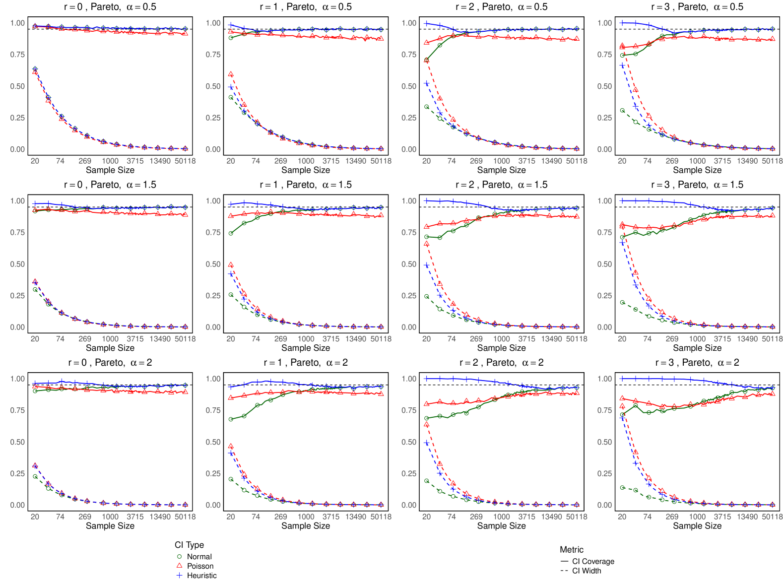
Discrete Pareto Distribution
We begin by recalling the continuous Pareto distribution. There are several parametrizations. We consider the one with the probability density function (pdf) given by
where is a parameter. We can simulate from this distribution by taking , where has a (continuous) uniform distribution on . We say that a random variable has a Discrete Pareto Distribution if , where denotes equality in distribution. In this case, the pmf is given by
It is readily checked that
From here, Proposition 4.1 in Chang & Grabchak (2023) implies that (3) and (4) hold for each . Thus, we always have asymptotic normality, and there is no need to consider a dynamic situation in this case.
Our simulation results are presented in Figure 4. We considered three choices for the parameter . From the plots we can see that the smaller the value of , the faster the coverage proportion of the Normal CI converges to . This is in keeping with other results that suggest that Turing’s estimator converges quicker for smaller values of , see Grabchak & Cosme (2017). We note that the Heuristic CI has very good performance. Once we are in a regime where the Normal CI is close to convergence, the Heuristic CI follows it closely. On the other hand, prior to convergence, the Heuristic CI outperforms the Normal CI in terms of the coverage proportion, sometimes significantly so. However, this is at the expense of having wider CIs.
4 Authorship Attribution and X (Twitter) Data
In this section, we present an application to the problem of authorship attribution. For an overview, see, e.g., Zhang & Huang (2007), Grabchak et al. (2013), Grabchak et al. (2018), Zheng et al. (2023), and the references therein. In this context, represents the common vocabulary consisting of all of the words that different authors can use. Associated with each author is a word-type distribution, , where for word , is the probability with which the author will use . In practice, it is usually difficult to estimate the word-type distribution. Instead, one typically estimates so-called diversity indices, which are functionals of the word-type distribution. Two of the most commonly used diversity indices are Shannon’s entropy Grabchak et al. (2013) and Simpson’s index Grabchak et al. (2018).
A common approach to authorship attribution is to consider two writing samples and to estimate one or more diversity indices for each sample. One then compares these estimated indices to see if they are statistically different from each other. Of course, such approaches do not take into account the order in which words are written, only their relative frequencies. While some information is lost, this does not seem to be a major issue; see the discussion in Grabchak et al. (2013). We now introduce our methodology for using Turing’s estimators for the problem of authorship attribution. It is motivated by, but different from, the approach of comparing diversity indices.
Let be the size of the first writing sample and be the size of the second writing sample. We denote the first sample as the corpus and the second as the testing set. The idea is to check if the testing set has too many (or too few) words that appear rarely (or never) in the corpus. Toward this end, for the corpus, we construct CIs for for , where . Then, for each , we calculate the detecting points
where is the number of words in the testing set that are observed exactly times in the corpus. We allow for repetition. Thus, if a word appears several times in the testing set, then each instance is counted separately when calculating . When , then is just the number of words (including repetitions) in the testing set that do not appear in the corpus. Next, we compare the detecting points with the corresponding CI. If, for most values of , falls inside the CI, it suggests that the writing samples are from the same author; while if most of them fall outside the CI, it suggests that the writing samples are from different authors.
To motivate this methodology, we note that is the probability of seeing a letter that is observed exactly times in the corpus. Thus, in a sample of size , we expect to see such words. It follows that
and hence
We now illustrate our methodology by applying it to real-world data. For simplicity and comparability, we calculate all CIs using the Normal CI given in (5). The data comes from X (formerly Twitter). The goal is to check if two X accounts are from the same author. This is important for the problem of identifying fake accounts. In this context, the writing samples are comprised of tweets from two accounts. These have been preprocessed to remove capitalization, punctuation, and URLs. Further, retweets are excluded from the data. All data in this section were obtained from Tareaf (2017); see also Tareaf et al. (2018).
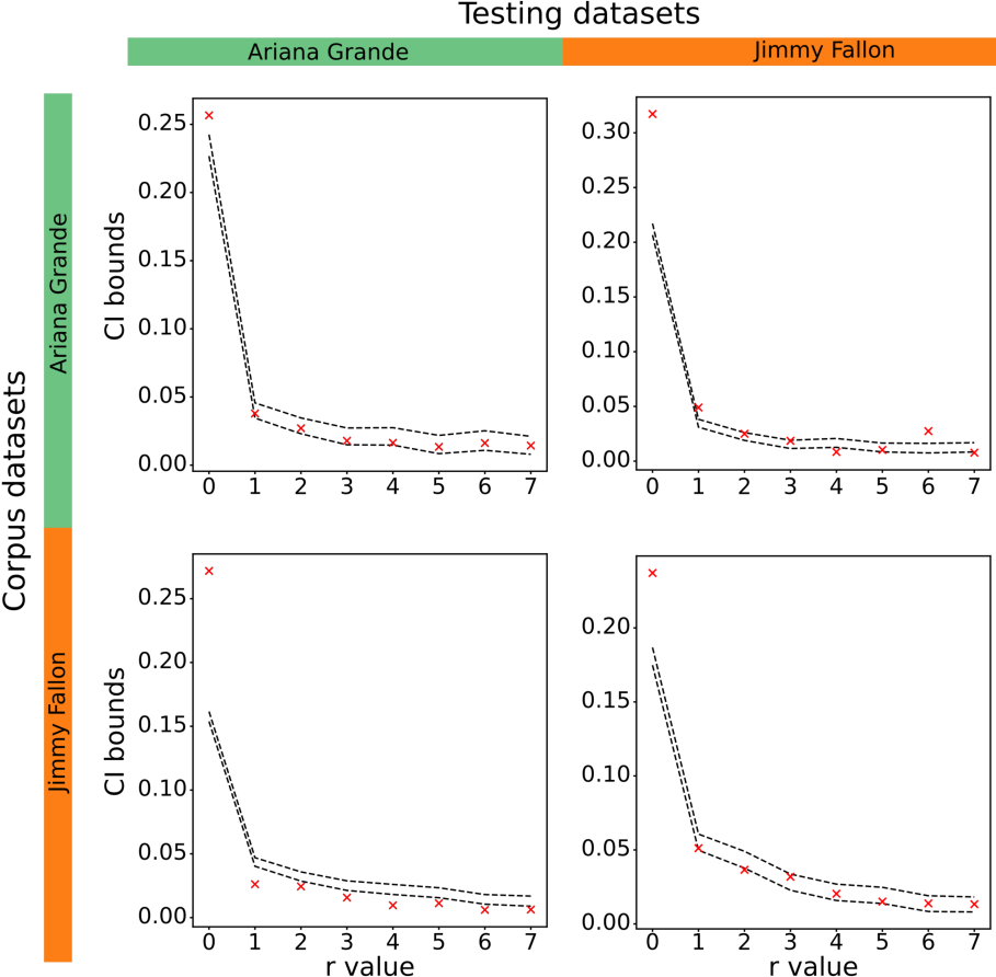
We begin by comparing two popular X users: Ariana Grande and Jimmy Fallon. The first sample consists of all tweets from Ariana Grande in 2015-2017 and the second consists of all tweets from Jimmy Fallon in 2013-2017. The sample from Ariana Grande contains words and the one from Jimmy Fallon contains words.
First, as a baseline, we compare each author’s writing with writing of the same author. Toward this end, we randomly divide each writing sample into two parts. We use one part as the corpus to construct the CIs and the other as the testing set. The results are given in the plots on the diagonal in Figure 5. We can see that most of the detecting points fall inside the CI, which indicates that the testing set is from the same author. The main exception is for . It seems that we have too many words in the testing set that do not appear in the corpus. This may be part of the nature of X, where certain topics and people become part of the zeitgeist for a short period of time and are just referred to in one tweet. Another reason may be related to when asymptotic normality holds for . Whatever the reason, these results suggest that, for authorship attribution in the context of X data, the use of values of is more relevant and seems to work well.
Next, we use the full writing sample from each author as the corpus to construct the CIs and the full writing sample from the other author as the testing set. The results are given in the off-diagonal plots in Figure 5. We see that most of the points fall outside the CI, which indicates that the testing set is from a different author. Note that things are not symmetric and that the detecting points seem to be further outside the CI when we use Jimmy Fallon’s tweets as the corpus than when we use Ariana Grande’s tweets.
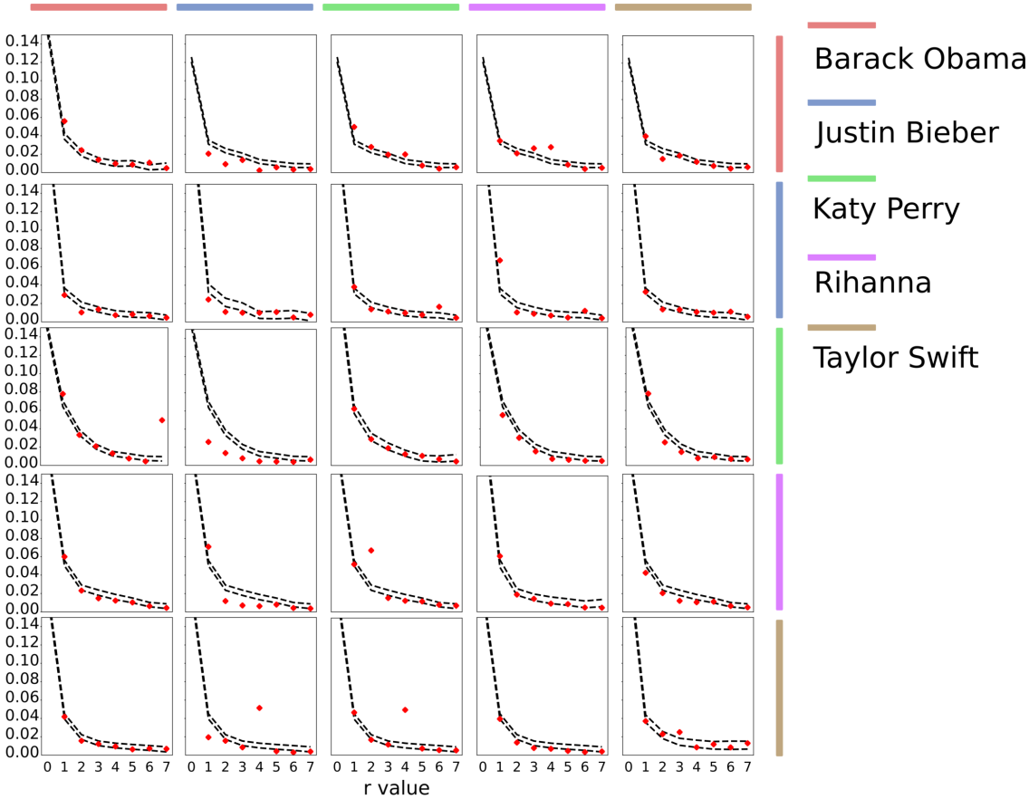
To better illustrate the methodology, we compare five of the top X (then Twitter) users in 2017. The results are given in Figure 6. The plots do not include , as these would make it hard to zoom in on the main parts of the plot, and, as we have seen, they do not seem to be relevant in the context of this application. Overall, the method seems to work well. However, in some cases, e.g., Justin Bieber, there are quite a few points that are outside the CI when comparing the authors to themselves. Similarly, there are situations where the method has difficulty distinguishing between two different authors, e.g., Justin Bieber and Taylor Swift.
5 Discussion
In this paper we performed a simulation study to compare the various CIs for the occupancy probabilities that appear in the literature. We also introduced the Heuristic CI, which aims to select the appropriate CI for a given random sample. We found that this CI works very well. Furthermore, we introduced a novel methodology for authorship attribution and applied it to several datasets from users of X (Twitter). Along the way, we proved several theoretical results, which give more context to our simulations and are interesting in their own right. We conclude with a brief summary/discussion of our simulation results from the perspective of heavy-tails.
It has been observed that Turing’s estimator tends to work better for heavier-tailed distributions than for lighter-tailed ones. Empirically, this was seen in the simulation study conducted in Grabchak & Cosme (2017), which considered the relative error of Turing’s estimator with . Theoretically, it is suggested by the fact that results for consistency and asymptotic normality of Turing’s estimator are only known for relatively heavy tailed distributions, see, e.g., Ohannessian & Dahleh (2012), Grabchak & Zhang (2017), or Chang & Grabchak (2023). The simulation results in the current paper echo this observation.
The discrete Pareto distribution has the heaviest tails out of all the distributions that we considered, and it is the only one for which asymptotic normality is known to hold. The parameter determines how heavy the tails are. The lower the value of , the heavier the tails. Our simulation results showed that the lower this value, the quicker the coverage proportion for the Normal CI approaches .
The geometric distribution has exponential tails, which are often considered to be on the boundary between heavy and light. The parameter determines how heavy the tails are, with lower values of leading to heavier tails. Our simulation results showed that the lower this value, the closer the coverage proportions for both the Normal CI and the Poisson CI are to , although they do not seem to approach this value. Asymptotic normality only holds in the dynamic case, where , i.e., as the tails get progressively heavier.
The discrete uniform distribution takes on only a finite number of possible values and is thus light-tailed. The parameter determines how heavy the tails are. The larger the value of , the heavier the tails. Our simulation results showed that the larger this value, the longer the period during which the Normal CI is close to in its pre-limit apparent convergence phase. Furthermore, we observed that asymptotic normality and asymptotic Poissonity only hold in the dynamic case, where , which is, again, as the tails get progressively heavier.
Appendix
Appendix A Conditions For Convergence
In this section, we summarize the known sufficient conditions for the convergence in (3), (4), and (7) to hold. Let be a sequence of probability distributions on the alphabet .
Proposition 3.
The first two parts are given in Theorems 2.1 and 2.3 of Chang & Grabchak (2023). The third is given in Theorem 1 of Zhang & Zhang (2009), see also Esty (1983). The following sufficient condition for (14) can be found in, e.g., Proposition 2.2 of Chang & Grabchak (2023).
Lemma 1.
If , then (14) holds.
Appendix B Proofs
B.1 Asymptotics for the Dynamic Uniform
In this section, we derive asymptotic results for the dynamic uniform distribution. Let be as in (11) and note that, in this case,
It is readily checked that for any
Thus, for , we have . It follows that for , we have
and for we have
Next, consider the case where . We have and , but . Thus Proposition 3 can only give us results for . In this case
Finally, we turn to the case . When , we have and
Thus, the conditions in Proposition 3 do not hold. Henceforth assume that . When we have and the conditions in Proposition 3 do not hold. When , we have . It follows that for any and large enough
Hence, (14) holds and Proposition 3 implies that (7) holds with . When , we have , , and . Thus, Proposition 3 implies that (3) and (4) hold in this case.
B.2 Proof of Proposition 2
Let for and note that for . Next, for , let for and let for . Note that . Since , is increasing on , decreasing on , and . Next, let and note that . Since is monotonically decreasing, it follows that is increasing on and decreasing on .
Lemma 2.
Assume that with .
1. We have
| (15) |
2. For any , we have
3. For any integer , we have
Proof.
First, note that 4.2.33 in Abramowitz & Stegun (1972) implies that for large enough , we have
and hence
Next, note that , , and , where we use (15) and the fact that as . By the Euler-Maclaurin Lemma, see e.g. Lemma 1.6 in Zhang (2017), we have
where we use the change of variables and (15). Turning to the third part, we have
which completes the proof. ∎
Lemma 3.
Proof.
Lemma 3 gives the second part of Proposition 2. We now turn to the first part. Henceforth assume that and . Lemma 2 implies that and . By Proposition 3, it suffices to show that (14) holds. Toward this end, note that for , thus when , we have for each . Henceforth, assume that . In this case, we have if and only if , where . Further, since , we have for large enough . It follows that, for such , is monotonically increasing for and
where we use the change of variables , dominated convergence, the fact that , the fact that as , and Lemma 2.
References
- (1)
- Abramowitz & Stegun (1972) Abramowitz, M. & Stegun, I. (1972), Handbook of Mathematical Functions, 10th edn, Dover Publications, New York.
- Chang & Grabchak (2023) Chang, J. & Grabchak, M. (2023), ‘Necessary and sufficient conditions for the asymptotic normality of higher order turing estimators’, Bernoulli 29(4), 3369–3395.
- Chao et al. (2015) Chao, A., Hsieh, T., Chazdon, R., Colwell, R. & Gotelli, N. (2015), ‘Unveiling the species-rank abundance distribution by generalizing the good–turing sample coverage theory’, Ecology 96(5), 1189–1201.
- Chao et al. (1988) Chao, A., Lee, S.-M. & Chen, T.-C. (1988), ‘A generalized good’s nonparametric coverage estimator’, Chinese Journal of Mathematics 16(3), 189–199.
- Decrouez et al. (2016) Decrouez, G., Grabchak, M. & Paris, Q. (2016), ‘Finite sample properties of the mean occupancy counts and probabilities’, Bernoulli 24(3), 1910–1941.
- Esty (1982) Esty, W. (1982), ‘Confidence intervals for the coverage of low coverage samples’, Annals of Statistics 10(1), 190–196.
- Esty (1983) Esty, W. (1983), ‘A normal limit law for a nonparametric estimator of the coverage of a random sample’, Annals of Statistics 11(3), 905–912.
- Good (1953) Good, I. (1953), ‘The population frequencies of species and the estimation of population parameters’, Biometrika 40(3/4), 237–264.
- Good (2000) Good, I. (2000), ‘Turing’s anticipation of empirical bayes in connection with the cryptanalysis of the naval enigma’, Journal of Statistical Computation and Simulation 66(2), 101–111.
- Gou et al. (2024) Gou, J., Ruth, K., Basickes, S. & Litwin, S. (2024), ‘A fortune cookie problem: A test for nominal data whether two samples are from the same population of equally likely elements’, Communications in Statistics-Theory and Methods 53(9), 3063–3077.
- Grabchak et al. (2018) Grabchak, M., Cao, L. & Zhang, Z. (2018), ‘Authorship attribution using diversity profiles’, Journal of Quantitative Linguistics 25(2), 142–155.
- Grabchak & Cosme (2017) Grabchak, M. & Cosme, V. (2017), ‘On the performance of turing’s formula: A simulation study’, Communications in Statistics – Simulation and Computation 46(6), 4199–4209.
- Grabchak & Samorodnitsky (2010) Grabchak, M. & Samorodnitsky, G. (2010), ‘Do financial returns have finite or infinite variance? a paradox and an explanation’, Quantitative Finance 10(8), 883–893.
- Grabchak & Zhang (2017) Grabchak, M. & Zhang, Z. (2017), ‘Asymptotic properties of turing’s formula in relative error’, Machine Learning 106(11), 1771–1785.
- Grabchak et al. (2013) Grabchak, M., Zhang, Z. & Zhang, D. (2013), ‘Authorship attribution using entropy’, Journal of Quantitative Linguistics 20(4), 301–313.
- Gupta et al. (1992) Gupta, V., Lennig, M. & Mermelstein, P. (1992), ‘A language model for very large-vocabulary speech recognition’, Computer Speech & Language 6(4), 331–344.
- Johnson et al. (2005) Johnson, N., Kemp, A. & Kotz, S. (2005), Univariate discrete distributions, 3rd edn, John Wiley & Sons, Hoboken.
- Lijoi et al. (2007) Lijoi, A., Mena, R. & Prünster, I. (2007), ‘A bayesian nonparametric method for prediction in est analysis’, BMC Bioinformatics 8(339), 1–10.
- Newton et al. (2014) Newton, P., Mason, J., Hurt, B., Bethel, K., Bazhenova, L., Nieva, J. & Kuhn, P. (2014), ‘Entropy, complexity and markov diagrams for random walk cancer models’, Scientific Reports 4(1), 7558.
- Ohannessian & Dahleh (2012) Ohannessian, M. & Dahleh, M. (2012), ‘Rare probability estimation under regularly varying heavy tails’, JMLR Workshop and Conference Proceedings 23, 21.1–21.24.
- Painsky (2023) Painsky, A. (2023), ‘Generalized good-turing improves missing mass estimation’, Journal of the American Statistical Association 118(543), 1890–1899.
- Pananjady et al. (2024) Pananjady, A., Muthukumar, V. & Thangaraj, A. (2024), ‘Just wing it: Near-optimal estimation of missing mass in a markovian sequence’, Journal of Machine Learning Research 25(312), 1–43.
- Robbins (1968) Robbins, H. (1968), ‘Estimating the total probability of the unobserved outcomes of an experiment’, Annals of Mathematical Statistics 39(1), 256–257.
- Sahai & Khurshid (1993) Sahai, H. & Khurshid, A. (1993), ‘Confidence intervals for the mean of a poisson distribution: A review’, Biometrical Journal 35(7), 857–867.
- Tareaf (2017) Tareaf, R. B. (2017), ‘Tweets dataset – top 20 most followed users in twitter social platform (version v2)’, Data set. Harvard Dataverse.
- Tareaf et al. (2018) Tareaf, R. B., Berger, P., Hennig, P. & Meinel, C. (2018), Malicious behaviour identification in online social networks, in S. Bonomi & E. Rivière, eds, ‘Distributed Applications and Interoperable Systems: DAIS 2018’, Vol. 10853 of Lecture Notes in Computer Science, Springer, Cham.
- Zhang & Zhang (2009) Zhang, C. & Zhang, Z. (2009), ‘Asymptotic normality of a nonparametric estimator of sample coverage’, Annals of Statistics 37(5A), 2582–2595.
- Zhang (2013) Zhang, Z. (2013), ‘A multivariate normal law for turing’s formulae’, Sankhya A 75(1), 51–73.
- Zhang (2017) Zhang, Z. (2017), Statistical Implications of Turing’s Formula, Wiley, Hoboken.
- Zhang (2018) Zhang, Z. (2018), ‘Domains of attraction on countable alphabets’, Bernoulli 24(2), 873–894.
- Zhang & Grabchak (2013) Zhang, Z. & Grabchak, M. (2013), ‘Bias adjustment for a nonparametric entropy estimator’, Entropy 15(6), 1999–2011.
- Zhang & Huang (2007) Zhang, Z. & Huang, H. (2007), ‘Turing’s formula revisited’, Journal of Quantitative Linguistics 14(2-3), 222–241.
- Zhang & Huang (2008) Zhang, Z. & Huang, H. (2008), ‘A sufficient normality condition for turing’s formula’, Journal of Nonparametric Statistics 20(5), 431–446.
- Zheng et al. (2023) Zheng, L., Zheng, H. & Kundu, C. (2023), ‘Authorship attribution via occupancy-problem-type indices’, Journal of Quantitative Linguistics 30(1), 27–41.